Article

Relative Contribution of Atmospheric Forcing, Oceanic Preconditioning and Sea Ice to Deep Convection in the Labrador Sea

School of Information Engineering, Nanjing Xiaozhuang University, Nanjing 211171, China
*
Authors to whom correspondence should be addressed.
J. Mar. Sci. Eng. 2023, 11(4), 869; https://doi.org/10.3390/jmse11040869
Submission received: 20 March 2023 / Revised: 17 April 2023 / Accepted: 18 April 2023 / Published: 20 April 2023
(This article belongs to the Special Issue Numerical Modelling of Atmospheres and Oceans II)

Abstract

:
The relative contribution of atmospheric forcing, oceanic preconditioning, and sea ice to Labrador Sea Deep Convection (LSDC) is investigated by conducting three ensemble experiments using a global coupled sea ice–ocean model for the first time. Simulated results show that the atmospheric activities dominate the interannual and decadal variability, accounting for 70% of LSDC. Oceanic preconditioning is more significant in the shallow LSDC years that the water column is stable, accounting for 21%, especially in the central Labrador Sea and Irminger Sea. Moreover, the sea ice contribution is negligible over the whole Labrador Sea, while its contribution is significant in the sea ice-covered slope regions, accounting for 20%. The increasingly importance of sea ice on LSDC and the water mass transformation will be found in the North Atlantic Ocean, if the Arctic sea ice declines continuously. Additionally, there is a 10 Sv increase (85%) in atmospheric forcing to the subpolar gyre in the North Atlantic Ocean, while oceanic preconditioning contributes a 7 Sv decrease (12%). These findings highlight the importance of summer oceanic preconditioning to LSDC and the subpolar gyre, and therefore it should be appropriately accounted for in future studies.

1. Introduction

The Labrador Sea is a pivotal region of open-ocean deep convection and deep water formation, connecting atmospheric forcing and deep ocean directly [1]. In winter, air–sea fluxes extract heat from the Labrador Sea intensively, resulting in the formation of Labrador Sea Water (LSW). LSW formation varies depending on multiple factors, including atmospheric activities, oceanic preconditioning, brine rejection caused by sea ice formation, and the inflow of freshwater from Greenland and the Nordic Seas [1,2,3]. A part of this water mass spreads equatorward as a component of North Atlantic Deep Water (NADW). It is generally considered to play an essential role in the variability of Atlantic meridional overturning circulation (AMOC), associated northward heat transport, and the global carbon cycle on decadal and longer time scales [4,5,6,7,8].
In the North Atlantic Ocean, North Atlantic Oscillation (NAO) is the leading mode of atmospheric forcing [9]. It modulates the westerlies in the subpolar North Atlantic and significantly influences LSW formation and Labrador Sea Deep Convection (LSDC) [10]. During a positive NAO phase, the enhanced westerlies, accompanied by a more significant number of high-frequency (<1 month) atmospheric activities and a shift of storm tracks [11], extract more oceanic heat from the Labrador Sea than that during a negative NAO phase, and thus prompt deep convection under favorable oceanic preconditioning [1,12]. The high-frequency atmospheric forcing (for example, storms, polar low and synoptic weather system) can also lead to significant variations in air–sea fluxes, LSW formation and LSDC [2,12,13,14,15,16,17,18]. However, the relationship between NAO and LSDC is not simply linear. For example, the enhanced deep convection in winter 2007/2008 (during a positive NAO phase) was influenced by complicated factors, including storms, freshwater fluxes, and the distribution of the ice pack [19]. In addition, the magnitude of air–sea fluxes in the Labrador Sea depends on the locations of the large-scale atmospheric circulation anomalies of the western North Atlantic, the Icelandic Low, and the spatial distribution of pack ice [18,20,21,22].
More recently, a gyre-scale deep convection was found in the subpolar North Atlantic Ocean driven by exceptional heat loss during winter 2014/2015 [23]. However, the late winter mixed layer depth (MLD) is shallower in the Irminger Sea (1400 m) than that in the Labrador Sea (1800 m) and south of Cape Farewell (1700 m), even though there is considerable winter heat loss in these regions [23]. A similar phenomenon, where MLD deepening stopped at 800–1000 m, was found in the Labrador Sea during winter 2007/2008 while the amount of heat loss was similar to that in winter 2014/2015 [23,24,25]. The subsequent question is why the exceptional heat loss did not deepen MLD in the subpolar North Atlantic Ocean. To address this question, the role of oceanic preconditioning (thermal and stratified state of the sea water) of water column and sea ice should be adequately considered. So far, only a limited number of studies have investigated the contribution of oceanic preconditioning to the convection event [1,26,27,28]. For example, Alverson (1995) studied the doming effect of oceanic stratification on deep convection. They found out that stratification with more sharply domed isopycnals produces deeper convective mixing. Straneo and Kawase (1999) investigated the relative contribution of domed isopycnals and localized buoyancy forcing to a subsequent convective event in the preconditioned ocean. They found almost equal importance of oceanic preconditioning and the buoyancy forcing to the convection events. Recently, Brakstad et al., (2019) found that the deeper convection in the Greenland Sea during winter was primarily the result of reduced water-column stability induced by increased near-surface salinity.
Meanwhile, ice cover can insulate heat loss from the ocean to the atmosphere, and then affects MLD [29]. For example, Våge et al., (2018) found that the re-ventilation of water mass is possibly caused by sea ice retreat toward Greenland when the water mass transits to the western Iceland Sea during winter; rigorous heat loss from the ocean offshore of the sea ice edge subsequently triggers deep convection [29]. Another effect of sea ice on MLD is brine rejection by sea ice formation to the near-surface salinity [28,30,31]. Moreover, the ongoing decline of Arctic sea ice extent increases freshwater inflow. It exposes the ocean to anomalous surface heat flux, resulting in positive buoyancy anomalies which can affect LSDC and AMOC [3,29,32]. For example, Yang et al., (2016) found that changes in LSW can be directly linked to recent freshening in the vicinity of the Greenland Sea and suggested a possible link to AMOC. Sévellec et al., (2017) investigated the sensitivity of AMOC to buoyancy flux perturbation over the Arctic Ocean. They found that flux anomalies over the subpolar North Atlantic have the most immense impact on AMOC on decadal time scales. In contrast, on multidecadal time scales, flux anomalies in the Arctic become more critical. However, a systematic study on the relative contribution of atmospheric forcing, oceanic preconditioning, and sea ice to LSDC is still lacking. Additionally, the subpolar North Atlantic (SPNA), which is characterized by the North Atlantic subpolar gyre, is a region where AMOC is actively developed and shaped though mixing and water mass transformation. The dynamics of the subpolar gyre are a result of strong buoyancy gradients, intense surface buoyancy and wind forcings, and exchange of waters with the Nordic Seas through overflows. Understanding these complex dynamics is essential to better understanding the mechanisms that drive the variability of AMOC. Changes in SPNA heat content and surface temperature are significant for many climate and weather phenomena, and biochemical processes [33,34].
Hence, three ensemble experiments are conducted to study the relative contribution of atmospheric forcing, oceanic precondition, and sea ice to LSDC by using the coupled global ocean–sea ice model. This paper is organized as follows. It begins in Section 2 with a brief description of the model setup and experimental design. The relative contribution to LSDC and its impacts are described quantitatively in Section 3. It closes with concluding remarks of our results in Section 4.

2. Model and Experimental Design

The MITgcm-ECCO2, which is the state estimate configuration Estimating the Circulation and Climate of the Ocean, phase 2, high-resolution global-ocean and sea-ice data synthesis, has been used to investigate the above questions [35,36]. To avoid the polar singularities, it employs a cube–sphere grid configuration to produce a relatively even grid size [37]. The model has a mean horizontal grid size of approximately 18 km (i.e., eddy permitting). There are 50 unevenly spaced vertical levels. Its vertical thickness increases from 10 m near the surface to 450 m at the ocean bottom. In addition, the ocean model is coupled with a sea ice model [38]; this coupled model is run with optimized control parameters by the Green Function approach [39]. We refer readers to Menemenlis et al., (2008) and Wu et al., (2016, 2020) for more details about the configuration of the ECCO2 state estimate [12,13,33,34].
We conducted a simulation for 1979–2017 (CTRL) with realistic atmospheric forcing derived from the Japanese 55-year reanalysis dataset [40]. Atmospheric forcing includes 6-hourly net short-wave and long-wave radiation, 2-m specific humidity, precipitation, 10-m wind velocity, and 2-m air temperature. The outputs from CTRL are used as the sea ice conditions and oceanic preconditions in the following ensemble experiments. As shown in the previous studies [41,42], LSDC reached a relatively low record in winter 2009/2010; and it reached a deep record in winter 2016/2017. It will be shown later that the water column in September 2009 is much more stable and that in 2016 is sharper than the climate oceanic state in September. Hence, the constant oceanic preconditioning in September 2009 is chosen in EXP-OP and EXP-SI, and two specific winters (2009/2010 and 2016/2017) were chosen to investigate the relative contribution of atmospheric forcing, oceanic preconditioning, and sea ice condition to LSDC. Three ensemble experiments with a respective 37 members in each experiment were conducted, in which atmospheric forcing (EXP-AT), oceanic preconditioning (EXP-OP), or sea ice forcing (EXP-SI) was switched to a fixed year at the beginning of each ensemble member (Table 1). Each ensemble member was integrated from September of one year to March of the following year, which is forced with data from a different single year and sea ice dataset details can be found in Table 1.
Specifically, the first member of EXP-AT (1 September 1979–31 March 1980) is driven by atmospheric forcing from 1 September of 1979 to 31 March of 1980. The monthly oceanic preconditioning in September 2009 of CTRL is used, and the sea ice condition is prescribed by the sea ice from 1 September 2009 to 31 March 2010 at the daily frequency. All the members in EXP-AT use the same oceanic preconditioning on September 2009 and sea ice forcing except using different levels of atmospheric forcing (Table 1). In the next ensemble experiments, the first member in EXP-OP (September 1979) is conducted by the monthly oceanic initial conditions on September 1979, and atmospheric forcing and sea ice condition from 1 September of 2016 to 1 March of 2017 (Table 1). All the ensemble members in EXP-OP use the same atmospheric forcing and sea ice condition except using different oceanic preconditioning. Similarly, the members in EXP-SI are conducted by the same atmospheric forcing (1 September 2009–31 March 2010) and monthly oceanic preconditioning (September 2009), but using different sea ice forcing (Table 1). In sum, the difference between the ensemble mean of EXP-AT and the results of winter 2009/2010 in CTRL is the contribution from atmospheric forcing to LSDC. Similarly, the difference between the ensembles mean of EXP-OP and winter 2016/2017 in CTRL, and the difference between the ensembles mean of EXP-SI and winter 2009/2010 in CTRL are defined as the contributions from oceanic preconditioning and the sea ice condition to LSDC, respectively.

3. Results and Discussion

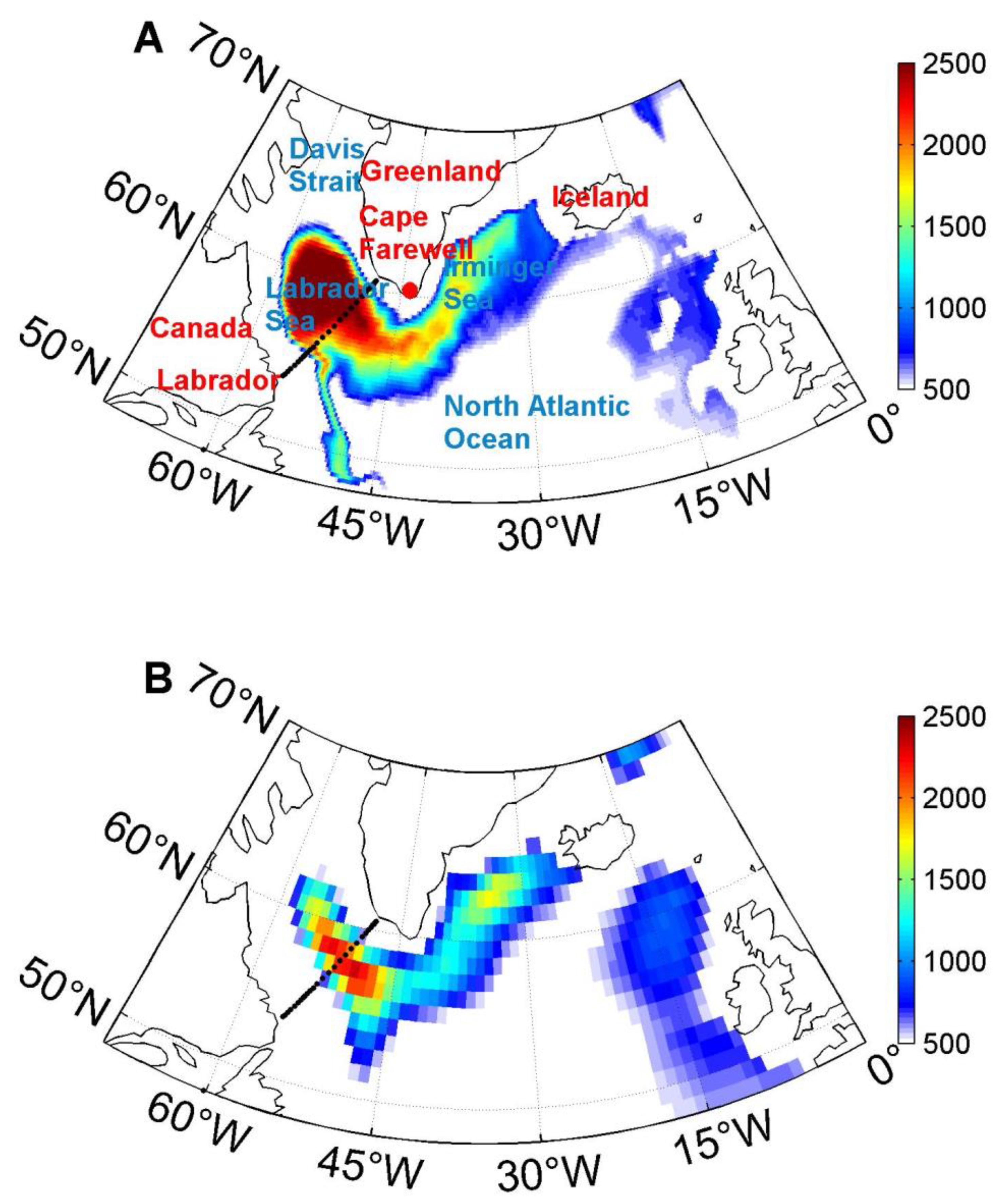
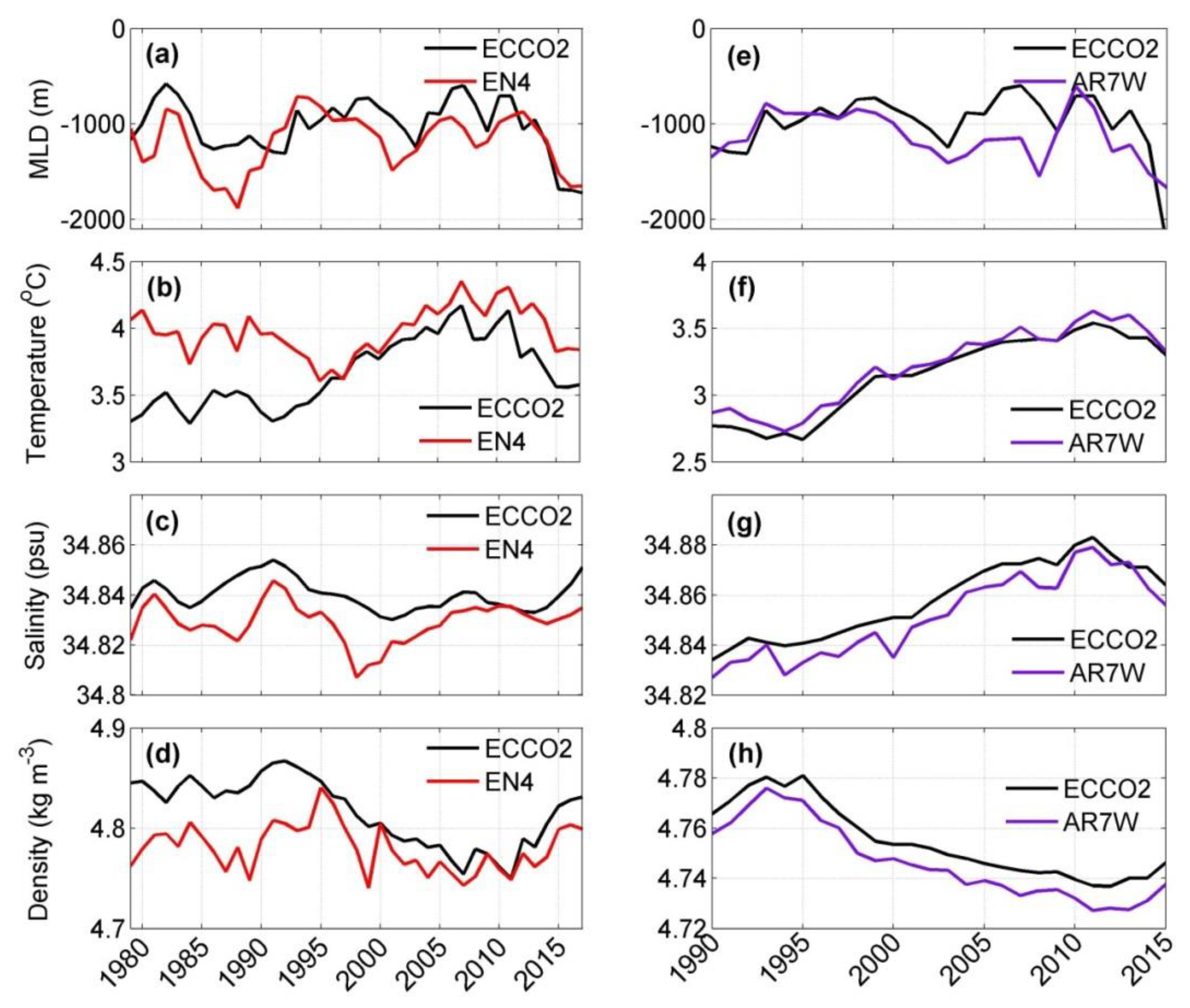
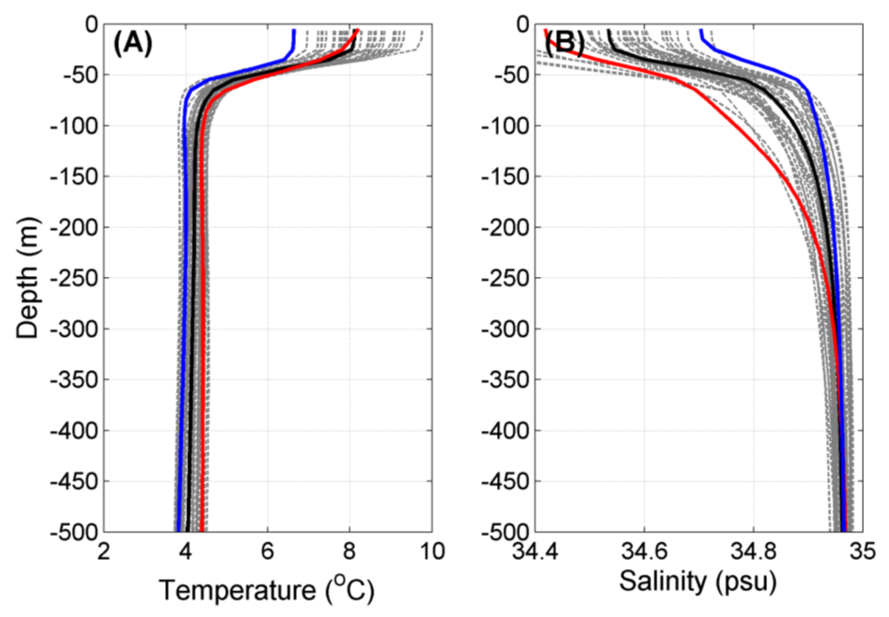
3.1. The Simulated Deep Convection in the Labrador Sea

To evaluate the realism of the simulated LSDC, Figure 1 presents the distributions of March-mean MLD in CTRL experiment (Figure 1A) and EN4 (Figure 1B) which is the global quality controlled ocean temperature and salinity profiles and monthly objective analyses within the 800-m isobath in the Labrador Sea averaged over 1979–2017. MLD is defined as the depth at which the potential density is 0.03 kg m−3 larger than that at the surface [13,43,44]. This density difference is larger than that used in Courtois et al. (2017), which may in part leads to deep MLD in our results (Figure 1) [45]. The simulated MLDs in ECCO2 and EN4 are characterized by large MLD in the central Labrador Sea (within the 2000-m isobath) and Irminger Sea (Figure 1), similar to the previous investigations [12,17,44]. It is noted that MLD in ECCO2 is deeper than that in EN4, due to lower surface salinity in EN4 than that in ECCO2 [44]. Meanwhile, the model resolution is relatively coarse, especially at the subpolar latitudes, and thus likely underestimates the role played by eddies in the restratification process after deep convection events [12,44,46,47,48,49]. Quantitatively, the time-mean MLDs averaged over the Labrador Sea (within the 800-m isobath) are 2750 m and 2340 m in ECCO2 and EN4, respectively, representing a 17.5% deeper MLD in ECCO2 than that in EN4. Overall, ECCO2 can represent the pattern of deep convection in the North Atlantic Ocean well, except the deeper MLD than that in the EN4.
Additionally, the model realistically reproduces the LSW properties compared to the EN4 analysis [50] and observational data along the AR7W section [51] averaged at the LSW depth (200–2000 m). Figure 2 shows good qualitative agreement between the observed and modeled LSDCs. Specifically, it shifts from a deep convection phase in the early-to-mid 1990s to a shallower intermediate phase during the late 1990s and mid-2000s, followed by the resumed deep convection in 2008 and the observed continued deepening of LSDC in winter 2012–2016 (Figure 2a,e) [42]. The 200–2000 m averaged temperature, salinity, and density time series over the central Labrador Sea region and along the AR7W section are presented in Figure 2b–d,f–h. The temperature, salinity, and density time series show significant multidecadal oscillations with an increase from 1979 to mid-1990s and a decrease (increase) in salinity and density (temperature) from mid-1990 to 2010s [41]; and, with an increase (decrease) in temperature and salinity (density) along the AR7W section (Figure 2f–h). In particular, density (temperature) increases (decreases) from 2012 to 2017 are consistent with the observational results [42]. These agreements indicate that the hind cast simulations in ECCO2 can indeed be used to explore the relative contribution of atmospheric forcing, oceanic preconditioning and sea ice on LSDC.
Figure 3 gives the simulated temperature and salinity profiles during September in CTRL, and the climatic September averaged within the central Labrador Sea over 1979–2017, which are strikingly similar to those of EN4 in magnitude, shape, and depth. The temperature and salinity profile slopes of 2009 are lower than the profile slope of climate. This reflects that the water column in September 2009 is much more stable than the time-mean oceanic state in September. As the finding in Figure 2a,e that the simulated and observed MLD in March 2010 reached a significantly low value, hence, oceanic preconditioning in September 2009 is selected to study the role played by atmospheric forcing in LSDC of the subsequent year. The temperature and salinity profiles in September 2016 are also given in Figure 3 which is much sharper than the other years, indicating a weaker stratification of water column.

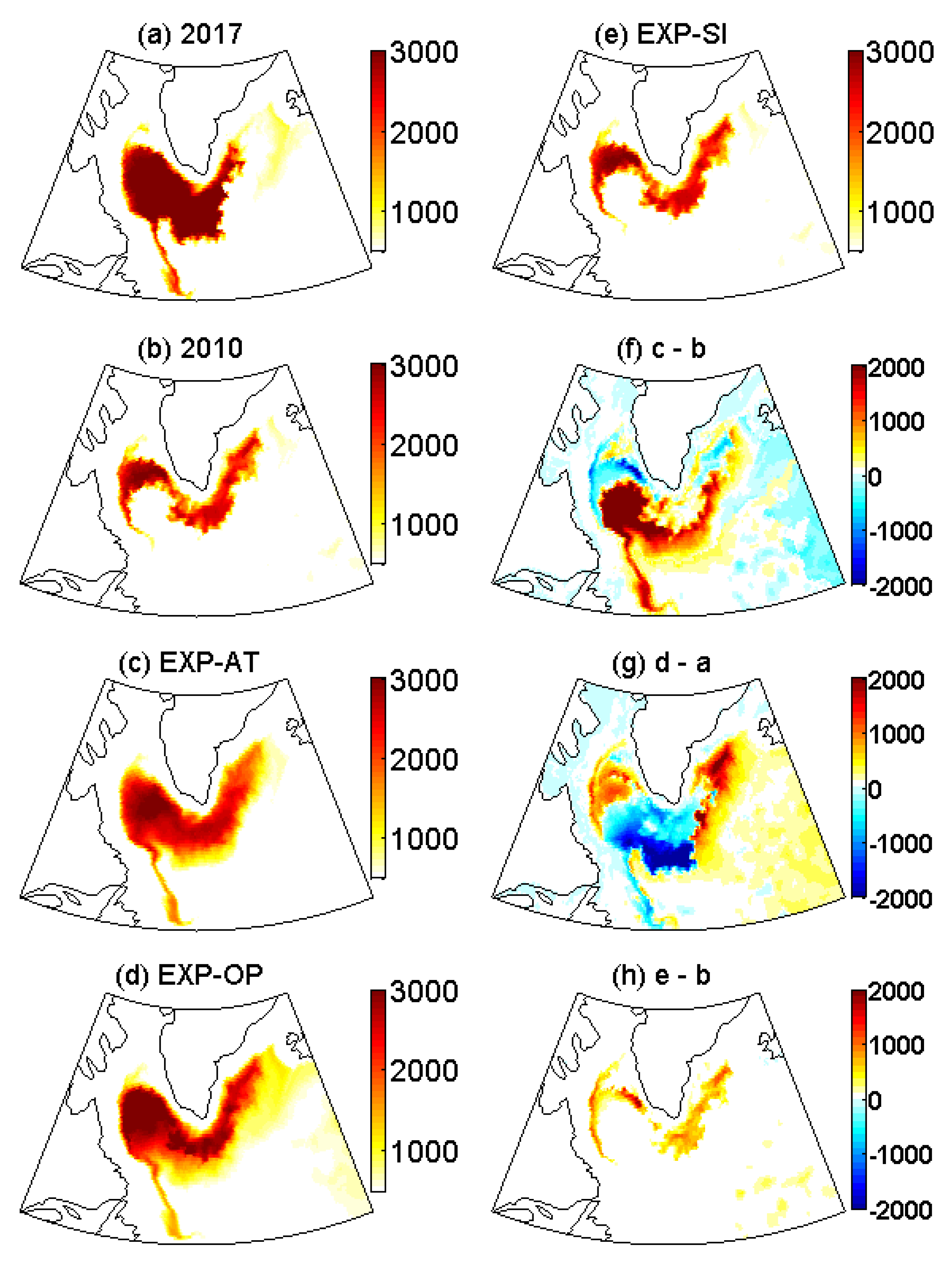
3.2. Relative Contributions of Atmospheric Forcing, Oceanic Preconditioning, and Sea Ice

Figure 4 presents the March-mean distributions of LSDC from CTRL and three ensemble simulations; and the differences between CTRL and three ensembles are also presented. Figure 4a shows the pattern of March-mean LSDC in 2017 which is characterized by deep MLD in the central Labrador Sea and the Irminger Sea. It is different from the pattern of March-mean LSDC in 2010 that the large MLD concentrates in the marginal regions along the Greenland (Figure 4b). Additionally, the March -mean and the ensemble mean distributions of LSDC in EXP-AT (Figure 4c) and EXP-OP (Figure 4d) are similar in that significant MLD is located in the central Labrador Sea and the Irminger Sea, except that there are deeper MLD in EXP-AT than that in EXP-OP over the central Labrador Sea and Irminger Sea. Meanwhile, Figure 4e gives the distribution of March-mean LSDC in EXP-SI which is similar to that in 2010 (Figure 4b) that large MLD concentrates in the slope regions along Greenland. As shown in the previous studies [3,29,32], the ensemble mean results of EXP-SI reflect the importance of sea ice in the slope region along Greenland.
Figure 4f presents the difference of March-mean LSDC between the ensemble results of EXP-AT and that of 2010 in CTRL. It presents the contribution of atmospheric forcing to LSDC which is characterized by a more than 1500-m positive difference in the central Labrador Sea and Irminger Sea and a more than 500-m negative difference in the marginal regions along the Greenland. Figure 4f shows that atmospheric forcing can almost reproduce deep convection in the central Labrador Sea and Irminger Sea, amounting to more than 1500 m from the beginning of the ocean heat loss in September. The negative values locate in the slope regions of the Labrador Sea and the Greenland Sea, which reflects the sea ice contribution to MLD there (Figure 4f), as in the previous investigations [3,29,32]. Figure 4g presents the spatial distributions of March LSDC difference between EXP-OP (Figure 4d) and that of 2017 (Figure 4a) which is characterized by negative values in the central Labrador Sea and the Irminger Sea, and positive values in the northeast Labrador Sea and the Nordic Sea. It indicates that the contribution of ocean preconditioning to LSDC is significant in the south of Greenland and Irminger Sea, amounting to more than 1000 m. This difference of LSDC is mainly induced by the stronger ocean stratification used in the ensemble experiment than that in September 2016. The influence of atmospheric forcing on LSDC is more extensive that dominating LSDC variability (Figure 4f), while the influence of oceanic preconditioning concentrates in the central Labrador Sea (Figure 4g). Figure 4h presents the difference between March-mean and ensemble-mean MLD in EXP-SI and March MLD of 2010 in CTRL. It indicates the sea ice contribution to LSDC which is more than 400 m in the marginal regions along the Greenland. The sea ice can isolate the heat lost in the winter season, and reduced sea ice extent and lower sea ice concentration in 2010 than that in CTRL causes deeper MLD there (Figure 4h).
The relative contribution of the three mentioned factors to LSDC is talked about in Figure 5. The percentage of contribution is defined as the difference of LSDC (averaged over the 800 m-isobaths) between each ensemble member and the selected year in CTRL divided by the corresponding value of the selected year in CTRL. The contribution of atmospheric forcing to LSDC is shown in Figure 5A which is from a relatively larger phase in the early-to-mid 1990s to a smaller phase during the late 1990s and mid-2000s, followed by the continuous larger contribution to the mid-2010s. This regime shift is similar to LSW thickness and the winter mean NAO index generally, since the correlation coefficient is 0.62 (0.53) between atmospheric forcing contribution and LSW thickness (winter mean NAO index), and 0.78 between LSW thickness and winter mean NAO index (Figure 5A). As in previous findings [12,17,18,23], LSDC is mainly induced by atmospheric forcing, accounting for more than 70% averaged from 1979 to 2015 (Figure 5A).
Figure 5B presents the contribution of oceanic preconditioning in September to the subsequent March LSDC in each ensemble member from 1979 to 2016. The MLD and oceanic preconditioning contribution presents an opposite trend generally. These results reveal significant variability over time from the maximum 41% contribution in 1999 to the minimum 3% contribution in 2016. On average, the percentage of the contribution of September oceanic preconditioning to March LSDC is 21%. The oceanic preconditioning contribution is significantly larger from the mid-1990s to the early 2000s, induced by the relatively stronger stratification and shallower MLD in that period (Figure 5B). Unlike the significant contribution of atmospheric forcing and oceanic preconditioning, sea ice condition is not a main forcing mechanism for the convective activity in the whole Labrador Sea, making a 4% contribution to LSDC (Figure 5C), on average, which is similar to the findings in Greenland Sea [28,53]. Additionally, the contribution of sea ice on MLD in the sea-ice-covered regions is shown in Figure 5C, indicating approximately 20% contribution to MLD there, and this contribution is more visible during the period of mid-1990s to 2017. It indicates that the role of sea ice will become more and more important to LSDC in North Atlantic Ocean as the Arctic sea ice declines continuously.

3.3. Impacts of the Relative Contributions on the North Atlantic Subpolar Gyre

The North Atlantic subpolar gyre plays a fundamental role in the global ocean circulation and the earth climate system [12]. It is also the key area where the warm and salty Atlantic water reaches to the Nordic Seas. Additionally, it modulates the atmospheric regimes (e.g., storm tracks) could be able to trigger climate variability by governing complex processes within the coupled ocean–atmosphere–ice system of the North Atlantic [12,13,44]. Hence, the impacts of the relative contribution to LSDC on the North Atlantic subpolar gyre have been studied here. Figure 6a,b presents the annual mean barotropic stream function in ocean of 2010 and 2017 in CTRL, which is characterized by cyclonic gyres in the North Atlantic Ocean and the Nordic Seas as that in the previous investigations [12,44,54]; and it can deliver the freshwater induced by the sea ice melting to the Labrador Sea and North Atlantic Ocean, and hence influence deep convection. Figure 6b shows that the strength of the simulated subpolar gyre reduces almost everywhere induced by the weaker wind stress curl in 2010 than that in 2017 (Figure 6a). For example, the strength of the subpolar gyre in the North Atlantic Ocean decreases by approximately 20.5% from 42.3 Sv in 2017 to 35.1 Sv in 2010. Similarly, the patterns of the ensemble mean subpolar gyres in EXP-AT (Figure 6c), EXP-OP (Figure 6d), and EXP-SI (Figure 6e) are also the same as that in CTRL. It is shown that atmospheric forcing dominates the variability of subpolar gyre over North Atlantic, especially in the central Labrador Sea, amounting to an 10 Sv increase (negative values in Figure 6f). The response of the subpolar gyre to the contribution of oceanic preconditioning is significant in the southeast of the North Atlantic Ocean, reaching a 7 Sv decrease (positive values in Figure 6g). Additionally, Figure 6 shows the influences of the contributions of atmospheric forcing, oceanic preconditioning, and sea ice to the North Atlantic subpolar gyre. These results show the significant impact of atmospheric forcing on the subpolar gyre amounting to 85% (Figure 6f), while oceanic preconditioning contributes 12% (7 Sv) to the subpolar gyre (Figure 6g). Meanwhile, the sea ice contribution to the subpolar gyre is negligible (Figure 6h).

4. Conclusions

LSDC connects the upper and deeper ocean directly, and plays a pivotal role in the air–sea ice–ocean interaction over the North Atlantic Ocean. In this study, the relative importance of atmospheric forcing, oceanic preconditioning, and sea ice to LSDC is investigated for the first time by using a global coupled ocean–sea ice model by conducting three ensemble experiments. Through comparing the numerical results, we found that:
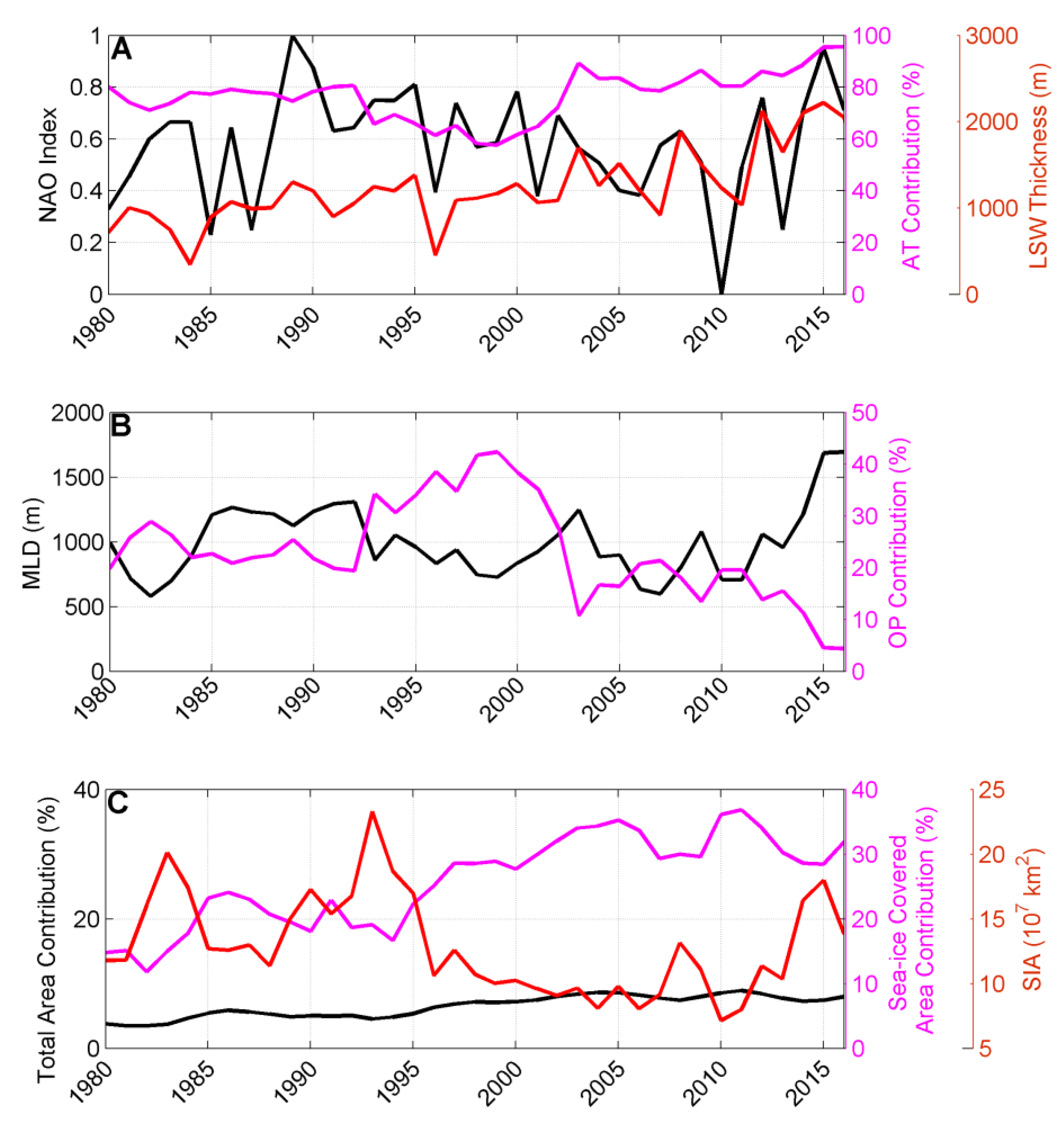
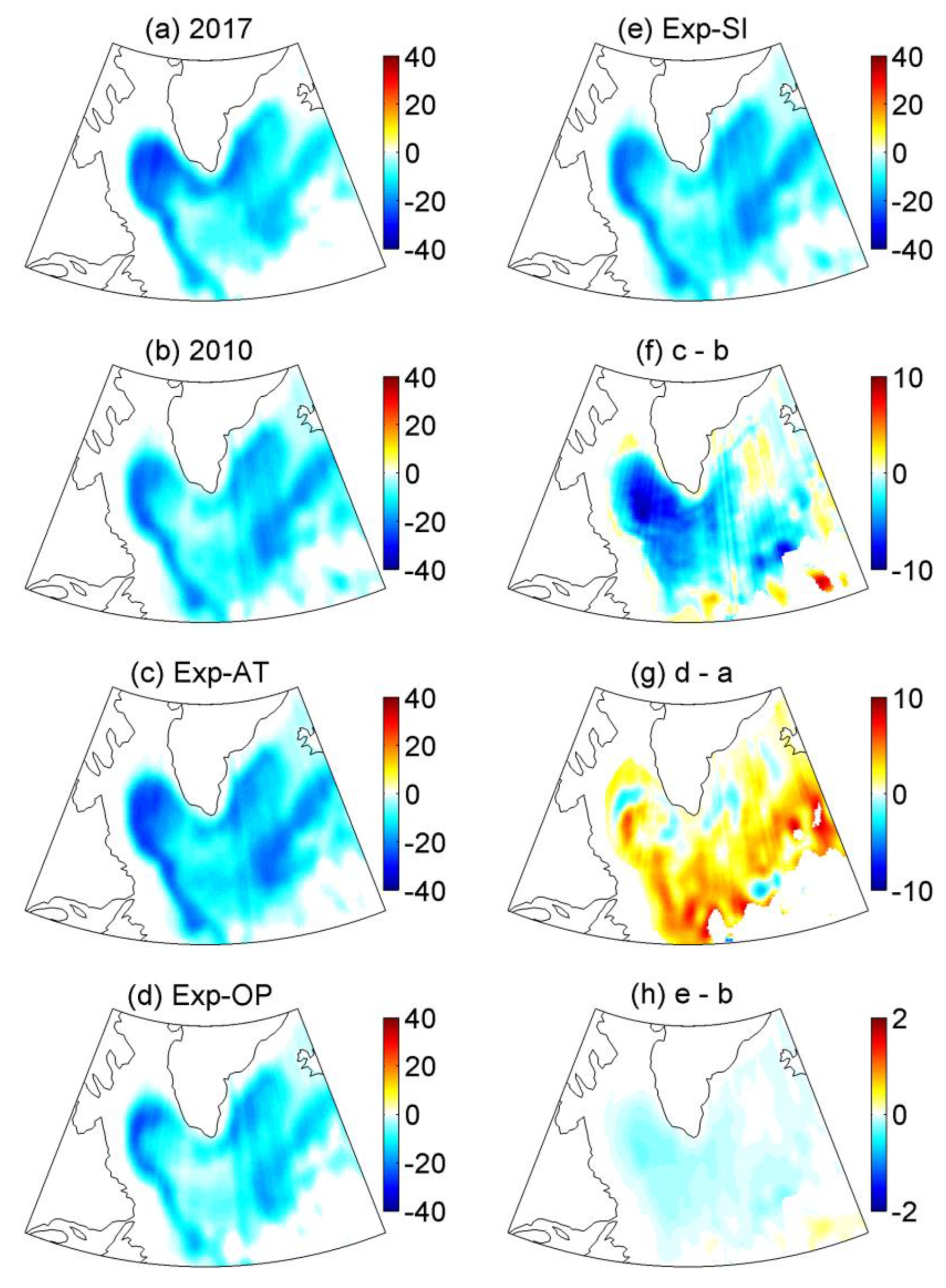
  • The simulated results show that atmospheric activities dominate the interannual and decadal variability. Its contribution accounts for more than 70% of LSDC, especially in the broad central Labrador Sea and the Irminger Sea.
  • The influence of oceanic preconditioning is more significant in the shallow LSDC years with strong oceean stratification, accounting for 21% on average. Moreover, the sea ice contribution is negligible for the region as a whole, while its contribution is significant in the sea ice-covered regions accounting for 20%.
  • The response of the North Atlantic subpolar gyre to the contribution of atmospheric forcing is different from the response of oceanic preconditioning that atmospheric forcing contributes an 85% increase in the North Atlantic subpolar gyre, while oceanic preconditioning presents a 12% decrease.
  • The observed and simulated anomalous lower LSDCs in specific winters are a result of the strong oceanic preconditioning which may induced by the delivered sea ice melting water by the North Atlantic subpolar gyre.
Although LSDC is jointly affected by these three mentioned factors, the relationship between these three factors is not simply linear, so when we diagnose the relative importance of these three factors, the total value will be more than 100%. LSDC connects atmospheric forcing and deep ocean directly, resulting in the formation of LSW, which plays an important role in AMOC variability, meridional heat transport, and the global carbon cycle, on decadal and longer time scales. Hence, the quantification of the relative contribution of atmospheric activities, oceanic preconditioning, and the sea ice to LSDC is important to the global ocean simulation. It is worth noting that this study has several limitations. For example, the model used here is only at the eddy-permitting resolution in the high latitudes. It is too coarse in the North Atlantic Ocean to resolve the eddy activities which are important in simulating deep convection. Additionally, the model used here is just a coupled ocean–sea ice model. The response of atmospheric forcing to ocean circulation is not included in the forcing. It needs to use a air–sea ice–ocean model to study this topic again in the future. Atmospheric forcing used here is relatively too coarse (six hourly mean, 1.125° × 1.125°) to resolve the high-frequency atmospheric activities which have been found to be very important to ocean surface fluxes [12,13].

Author Contributions

Conceptualization, Y.W. and X.Z.; model, Y.W.; investigation, Y.W. and X.Z.; resources, Z.Q., K.Z. and D.Q.; writing—review and editing, Y.W. and X.Z.; visualization, Y.W. and K.Z.; funding acquisition, Y.W. All authors have read and agreed to the published version of the manuscript.

Funding

This research was funded by the National Natural Science Foundation of China, grant numbers 41806216 and 62177028; by the Natural Science Foundation of Jiangsu Province, grant number BK20211015; by the China Postdoctoral Science Foundation, grant numbers 2019T120379 and 2018M630499; and by the Talent start-up fund of Nanjing Xiaozhuang University, grant number 4172111.

Institutional Review Board Statement

Not applicable.

Informed Consent Statement

Not applicable.

Data Availability Statement

The data presented in this study are available on request from the corresponding author.

Acknowledgments

The MITgcm code was obtained freely from http://mitgcm.org/. The atmospheric forcing data were obtained freely from the NCAR’s research data archive (JRA-55: https://rda.ucar.edu/datasets/ds625.0/, accessed on 1 March 2023.). The EN4 data were obtained freely from: https://www.metoffice.gov.uk/hadobs/en4/download-en4-2-1.html (accessed on 1 March 2023) Additionally, the observations of the AR7W section were obtained from: https://www.ncei.noaa.gov/access/ocean-carbon-data-system/oceans/RepeatSections/clivar_ar07w.html (accessed on 1 March 2023).

Conflicts of Interest

The authors declare no conflict of interest.

References

  1. Marshall, J.; Schott, R. Open ocean deep convection: Observations, theory, and models. Rev. Geophys. 1999, 37, 1–64. [Google Scholar] [CrossRef]
  2. Våge, K.; Pickart, R.S.; Thierry, V.; Reverdin, G.; Lee, C.M.; Petrie, B.; Agnew, T.A.; Wong, A. Surprising return of deep convection to the subpolar North Atlantic Ocean in winter 2007–2008. Nat. Geosci. 2009, 2, 67–72. [Google Scholar] [CrossRef]
  3. Yang, Q.; Dixon, T.H.; Myers, P.G.; Bonin, J.; Chambers, D.; van den Broeke, M.R.; Ribergaard, M.H. Recent increases in Arctic freshwater flux affects Labrador Sea convection and Atlantic overturning circulation. Nat. Commun. 2016, 7, 10525. [Google Scholar] [CrossRef] [PubMed]
  4. Eden, C.; Willebrand, J. Mechanism of interannual to decadal variability of the North Atlantic circulation. J. Clim. 2001, 14, 2266–2280. [Google Scholar] [CrossRef]
  5. Böning, C.W.; Scheinert, M.; Dengg, J.; Biastoch, A.; Funk, A. Decadal variability of subpolar gyre transport and its reverberation in the North Atlantic overturning. Geophys. Res. Lett. 2006, 33, L21S01. [Google Scholar] [CrossRef]
  6. Yeager, S.; Danabasoglu, G. The origins of late-twentieth-century variations in the large-scale North Atlantic circulation. J. Clim. 2014, 27, 3222–3247. [Google Scholar] [CrossRef]
  7. Srokosz, M.A.; Bryden, H.L. Observing the Atlantic Meridional Overturning Circulation yields a decade of inevitable surprises. Science 2015, 348, 1255575. [Google Scholar] [CrossRef]
  8. Buckley, M.W.; Marshall, J. Observations, inferences, and mechanisms of the Atlantic Meridional Overturning Circulation: A review. Rev. Geophys. 2016, 54, 5–63. [Google Scholar] [CrossRef]
  9. Hurrell, J.W. Decadal trends in the North Atlantic Oscillation: Regional temperatures and precipitation. Science 1995, 269, 676–679. [Google Scholar] [CrossRef]
  10. Yashayaev, I. Hydrographic changes in the Labrador Sea, 1960–2005. Prog. Oceanogr. 2007, 73, 242–276. [Google Scholar] [CrossRef]
  11. Dickson, R.R.; Lazier, J.; Meincke, J.; Rhines, P.; Swift, J. Long-term coordinated changes in the convective activity of the North Atlantic. Prog. Oceanogr. 1996, 38, 241–295. [Google Scholar] [CrossRef]
  12. Wu, Y.; Zhai, X.; Wang, Z. Impact of synoptic atmospheric forcing on the mean ocean circulation. J. Clim. 2016, 29, 5709–5724. [Google Scholar] [CrossRef]
  13. Wu, Y.; Wang, Z.M.; Liu, C.Y.; Lin, X. Impacts of high-frequency atmospheric forcing on Southern Ocean circulation and Antarctic sea ice. Adv. Atmos. Sci. 2020, 37, 515–531. [Google Scholar] [CrossRef]
  14. Zhai, X.; Johnson, H.L.; Marshall, D.P.; Wunsch, C. On the wind power input to the ocean general circulation. J. Phys. Oceanogr. 2012, 42, 1357–1365. [Google Scholar] [CrossRef]
  15. Condron, A.; Renfrew, I.A. The impact of polar mesoscale storms on northeast Atlantic Ocean circulation. Nat. Geosci. 2013, 6, 34–37. [Google Scholar] [CrossRef]
  16. Jung, T.; Serrar, S.; Wang, Q. The oceanic response to mesoscale atmospheric forcing. Geophys. Res. Lett. 2014, 41, 1255–1260. [Google Scholar] [CrossRef]
  17. Holdsworth, A.M.; Myers, P.G. The Influence of High-Frequency Atmospheric Forcing on the Circulation and Deep Convection of the Labrador Sea. J. Clim. 2015, 28, 4980–4996. [Google Scholar] [CrossRef]
  18. Kim, M.; Yeager, S.; Chang, P.; Danabasoglu, G. Atmospheric conditions associated with labrador sea deep convection: New insights from a case study of the 2006/07 and 2007/08 winters. J. Clim. 2016, 29, 5281–5297. [Google Scholar] [CrossRef]
  19. Yashayaev, I.; Loder, J.W. Enhanced production of labrador sea water in 2008. Geophys. Res. Lett. 2009, 36, L01606. [Google Scholar] [CrossRef]
  20. Serreze, M.C.; Carse, R.; Barry, R. Icelandic low cyclone activity: Climatological features, linkage with the NAO, and relationships with recent changes in the Northern Hemisphere circulation. J. Clim. 1997, 10, 453–464. [Google Scholar] [CrossRef]
  21. Moore, G.W.K.; Renfrew, I.A.; Pickart, R.S. Multidecadal mobility of the North Atlantic Oscillation. J. Clim. 2013, 26, 2453–2466. [Google Scholar] [CrossRef]
  22. Moore, G.W.K.; Pickart, R.S.; Renfrew, I.A.; Vage, K. What causes the location of the air-sea turbulent heat flux maximum over the Labrador Sea? Geophys. Res. Lett. 2014, 41, 3628–3635. [Google Scholar] [CrossRef]
  23. Piron, A.; Thierry, V.; Mercier, H.; Caniaux, G. Gyre-scale deep convection in the subpolar North Atlantic Ocean during winter 2014–2015. Geophys. Res. Lett. 2017, 44, 1439–1447. [Google Scholar] [CrossRef]
  24. Våge, K.; Pickart, R.S.; Moore, G.W.K.; Ribergaard, M.H. winter mixed layer development in the central Irminger Sea: The effect of strong, intermittent wind events. J. Phys. Oceanogr. 2008, 38, 541–565. [Google Scholar] [CrossRef]
  25. De Jong, M.F.; van Aken, H.M.; Våge, K.; Pickart, R.S. Convective mixing in the central Irminger Sea: 2002–2010. Deep Sea Res. Part I Oceanogr. Res. Pap. 2012, 63, 36–51. [Google Scholar] [CrossRef]
  26. Alverson, K.D. Topographic Preconditioning of Open-Ocean Deep Convection. Ph.D. Thesis, Massachusetts Institute of Technology, Cambridge, MA, USA, 1995; 146p. [Google Scholar]
  27. Straneo, F.; Kawase, M. Comparison of localized convection due to localized forcing and to preconditioning. J. Phys. Oceanogr. 1999, 29, 55–68. [Google Scholar] [CrossRef]
  28. Brakstad, A.; Våge, K.; Håvik, L.; Moore, G.W.K. Water mass transformation in the Greenland Sea during the period 1986–2016. J. Phys. Oceanogr. 2019, 49, 121–140. [Google Scholar] [CrossRef]
  29. Våge, K.; Papritz, L.; Håvik, L.; Spall, M.A.; Moore, G.W.K. Ocean convection linked to the recent ice edge retreat along east Greenland. Nat. Commun. 2018, 9, 1287. [Google Scholar] [CrossRef]
  30. Ronski, S.; Budéus, G. Time series of winter convection in the Greenland Sea. J. Geophys. Res. 2005, 110, C04015. [Google Scholar] [CrossRef]
  31. Latarius, K.; Quadfasel, D. Seasonal to inter-annual variability of temperature and salinity in the Greenland Sea gyre: Heat and freshwater budgets. Tellus A 2010, 62, 497–515. [Google Scholar] [CrossRef]
  32. Sévellec, F.; Alexey, F.V.; Liu, W. Arctic sea-ice decline weakens the Atlantic Meridional Overturning Circulation. Nat. Clim. Change 2017, 7, 604–610. [Google Scholar] [CrossRef]
  33. Wu, Y.; Zhai, X.M.; Wang, Z.M. Decadal-mean impact of including ocean surface currents in bulk formulas on surface air-sea fluxes and ocean general circulation. J. Clim. 2017, 30, 9511–9525. [Google Scholar] [CrossRef]
  34. Wu, Y.; Wang, Z.; Liu, C.; Yan, L. Energetics of Eddy-Mean Flow Interactions in the Amery Ice Shelf Cavity. Front. Mar. Sci. 2021, 8, 638741. [Google Scholar] [CrossRef]
  35. Marshall, J.; Adcroft, A.; Hill, C.; Perelman, L.; Heisey, C. A finite-volume, incompres- sible Navier Stokes model for studies of the ocean on parallel computers. J. Geophys. Res. 1997, 102, 5753–5766. [Google Scholar] [CrossRef]
  36. Marshall, J.; Hill, C.; Perelman, L.; Adcroft, A. Hydrostatic, quasi-hydrostatic, and nonhydrostatic ocean modeling. J. Geophys. Res. 1997, 102, 5733–5752. [Google Scholar] [CrossRef]
  37. Adcroft, A.; Campin, J.M.; Hill, C.; Marshall, J. Implementation of an atmosphere- ocean general circulation model on the expanded spherical cube. Mon. Weather Rev. 2004, 132, 2845–2863. [Google Scholar] [CrossRef]
  38. Losch, M.; Menemenlis, D.; Heimbach, P.; Campin, J.; Hill, C. On the formulation of sea-ice models. Part 1: Effects of different solver implementations and parameterizations. Ocean Model. 2010, 33, 129–144. [Google Scholar] [CrossRef]
  39. Menemenlis, D.; Campin, J.; Heimbach, P.; Hill, C.; Lee, T.; Nguyen, A.; Schodlok, M.; Zhang, H. ECCO2: High resolution global ocean and sea ice data synthesis. In Proceedings of the American Geophysical Union, Fall Meeting 2008, San Francisco, CA, USA, 15–19 December 2008; Volume 31, pp. 13–21. [Google Scholar]
  40. Kobayashi, S.; Ota, Y.; Harada, Y.; Ebita, A.; Moriya, M.; Onoda, H.; Onogi, K.; Kamahori, H.; Kobayashi, C.; Endo, H.; et al. The JRA-55 reanalysis: General specifications and basic characteristics. J. Meteor. Soc. Jpn. 2015, 93, 5–48. [Google Scholar] [CrossRef]
  41. Yashayaev, I.; Loder, J.W. Recurrent replenishment of Labrador Sea Water and associated decadal-scale variability. J. Geophys. Res. 2016, 121, 8095–8114. [Google Scholar] [CrossRef]
  42. Yashayaev, I.; Loder, J.W. Further intensification of deep convection in the labrador sea in 2016. Geophys. Res. Lett. 2017, 44, 1429–1438. [Google Scholar] [CrossRef]
  43. Downes, S.M.; Bindoff, N.L.; Rintoul, S.R. Impacts of climate change on the subduction of mode and intermediate water masses in the Southern Ocean. J. Clim. 2009, 22, 3289–3302. [Google Scholar] [CrossRef]
  44. Wu, Y.; Wang, Z.; Liu, C. Impacts of Changed Ice-Ocean Stress on the North Atlantic Ocean: Role of Ocean Surface Currents. Front. Mar. Sci. 2021, 8, 628892. [Google Scholar] [CrossRef]
  45. Courtois, P.; Hu, X.; Pennelly, C.; Spence, P.; Myers, P.G. Mixed layer depth calculation in deep convection regions in ocean numerical models. Ocean Model. 2017, 120, 60–78. [Google Scholar] [CrossRef]
  46. Rattan, S.; Myers, P.G.; Treguier, A.-M.; Theetten, S.; Biastoch, A.; Böning, C. Towards an understanding of labrador sea salinity drift in eddy-permitting simulations. Ocean Modell. 2010, 35, 77–88. [Google Scholar] [CrossRef]
  47. Marzocchi, A.; Hirschi, J.J.M.; Holliday, N.P.; Cunningham, S.A.; Blaker, A.T.; Coward, A.C. The North Atlantic subpolar circulation in an eddy-resolving global ocean model. J. Mar. Syst. 2015, 142, 126–143. [Google Scholar] [CrossRef]
  48. Rieck, J.K.; Böning, C.W.; Getzlaff, K. The nature of eddy kinetic energy in the labrador sea: Different types of mesoscale eddies, their temporal variability and impact on deep convection. J. Phys. Oceanogr. 2019, 49, 2075–2094. [Google Scholar] [CrossRef]
  49. Pennelly, C.; Myers, P.G. Introducing LAB60: A 1/60° NEMO 3.6 numerical simulation of the Labrador Sea. Geosci. Model Dev. 2020, 13, 4959–4975. [Google Scholar] [CrossRef]
  50. Good, S.A.; Martin, M.J.; Rayner, N.A. EN4: Quality controlled ocean temperature and salinity profiles and monthly objective analyses with uncertainty estimates. J. Geophys. Res. 2013, 118, 6704–6716. [Google Scholar] [CrossRef]
  51. Lazier, J.; Hendry, R.; Clarke, A.; Yashayaev, I.; Rhines, P. Convection and restratification in the Labrador Sea, 1990–2000. Deep Sea Res. Part I Oceanogr. Res. Pap. 2002, 49, 1819–1835. [Google Scholar] [CrossRef]
  52. Stramma, L.; Kieke, D.; Rhein, M.; Schott, F.; Yashayaev, I.; Koltermann, K.P. Deep water changes at the western boundary of the subpolar North Atlantic during 1996–2001. Deep Sea Res. Part I Oceanogr. Res. Pap. 2004, 51, 1033–1056. [Google Scholar] [CrossRef]
  53. Moore, G.; Våge, K.; Pickart, R.; Renfrew, I.A. Decreasing intensity of open-ocean convection in the Greenland and Iceland seas. Nat. Clim. Chang. 2015, 5, 877–882. [Google Scholar] [CrossRef]
  54. Wu, Y.; Wang, Z.M.; Liu, C. On the response of the Lorenz energy cycle for the Southern Ocean to intensified westerlies. J. Geophys. Res. 2017, 122, 2465–2493. [Google Scholar] [CrossRef]
Figure 1. The spatial distributions of March-mean MLD (m) in ECCO2 (A) and EN4 (B) averaged over 1979–2017. The AR7W section is labelled by the black dotted line. The geographical and sea names are also labeled in (A).
Jmse 11 00869 g001
Figure 2. (Left column) Time series of EN4 (red lines) and ECCO2 (black lines) (a) MLD, (b) temperature, (c) salinity, and (d) density averaged over the central Labrador Sea region (within the 2000−m isobath) at the LSW depth between 200 and 2000 m. Values in (d) and (h) minus 23. (Right column, (eh)) As in the left column, but for the data collected along the AR7W section. Note that the modeled LSW is slightly denser than observed induced by the slightly higher modeled salinity. The LSW is defined as Stramma et al., (2004) [52] that is bound by the isopycnals σΘ = [27.68, 27.80] kg m−3.
Jmse 11 00869 g002
Figure 3. Simulated profiles of temperature (A) and salinity (B) in September of 2009 (red), 2016 (blue) and climatic September (black) averaged over 1979–2016 within the 2000 m isobaths in CTRL. The simulated profiles of temperature and salinity in other years (grey dotted lines) are also given.
Jmse 11 00869 g003
Figure 4. The distributions of March MLD of 2017 (a) and 2010 (b) in CTRL; and the ensemble mean of the March MLD in EXP−AT (c), EXP−OP (d), and EXP−SI (e); and the differences between the CTRL and ensemble mean experiments: c minus b (f), d minus a (g), and e minus b (h).
Jmse 11 00869 g004
Figure 5. The relative contributions (%; magenta lines) of atmospheric forcing (A), oceanic preconditioning (B), and sea ice (C) to deep convection in the Labrador Sea. The red and black lines in (A) are LSW thickness (m) in the CTRL and the NAO index, respectively. The black line in (B) is the mixed layer depth (m). Additionally, the red line in (C) is the sea ice area that used in the ensemble members of EXP-SI; the solid black line in (C) is the sea ice contribution to deep convection in the Labrador Sea calculated over the whole region. The curve corresponds to the Y-axis of the same color.
Jmse 11 00869 g005
Figure 6. The same as in Figure 4, but for the barotropic stream function (Sv).
Jmse 11 00869 g006
Table 1. Summary of numerical experiments.
ExperimentsAtmospheric
Forcing
Oceanic
Preconditioning
Sea Ice
CTRL1979–2017
EXP-AT1 September 1979–31 March 1980

1 September 2016–31 March 2017
September 20091 September 2009–31 March 2010
EXP-OP1 September 2016–31 March 2017September 1979

September 2016
1 September 2016–31 March 2017
EXP-SI1 September 2009–31 March 2010September 20091 September 1979–31 March 1980

1 September 2016–31 March 2017
Disclaimer/Publisher’s Note: The statements, opinions and data contained in all publications are solely those of the individual author(s) and contributor(s) and not of MDPI and/or the editor(s). MDPI and/or the editor(s) disclaim responsibility for any injury to people or property resulting from any ideas, methods, instructions or products referred to in the content.

