Interannual Variability and Long-Term Trends in Intensity of the Yellow Sea Cold Water Mass during 1993–2019

Abstract

The Yellow Sea Cold Water Mass (YSCWM) is an important component of the hydrodynamic system and it significantly impacts the primary production of the Yellow Sea. This study investigated the difference in the interannual variability and long-term trends between the northern YSCWM (NYSCWM) and southern YSCWM (SYSCWM), and explored the main physical environmental factors that led to their inconsistency using multiple wavelet coherence. On the interannual scale, the intensities of the NYSCWM and SYSCWM exhibited consistent variability, but the intensity of the SYSCWM had a larger standard deviation and longer periodic signal than that of the NYSCWM. The two-factor combination of surface air temperature (SAT)–Niño 3.4 in the NYSCWM and sea surface temperature (SST)–northward seawater velocity (Vgos) in the SYSCWM controlled the interannual variability, which meant the influencing intensity variability differed in the NYSCWM and SYSCWM. In the long-term trend, the intensities of the NYSCWM and SYSCWM both showed decreasing trends during the study period. However, the enhanced circulation provided more horizontal heat input into the SYSCWM, and the relatively higher increase in SST and decrease in the amplitude of variation in the thermocline depth promoted vertical heat exchange in the SYSCWM, thereby making the intensity of the SYSCWM decrease more quickly than that of the NYSCWM. These findings provide important references that facilitate a deeper understanding of the influence of hydrological processes on marine ecosystems in marginal seas.

1. Introduction

The marine ecosystem plays an important role in the global carbon cycle and in climate warming [1]. Cold water masses, also known as “cold pools”, have been widely observed in shelf seas [2,3]. Cold waters from the previous winter are locally trapped in a topographic depression after the onset of seasonal stratification, for example, the cold water masses in the Irish Sea [4], Middle Atlantic Bight [5], North Sea [6,7] and the Yellow Sea (YS) [8,9]. There are strong temperature gradients between cold water masses and surrounding waters, which generate special hydrodynamic processes, such as cyclonic circulation above the cold water mass [3,10]. The upwelling formed by the vertical circulation and temperature changes in the cold water masses profoundly affects the phytoplankton production process, resulting in high primary phytoplankton productivity and abundant fishery resources [11,12]. Therefore, the intensity variabilities of cold water masses significantly impact the marine ecosystem [13,14].

The Yellow Sea (YS) is a shallow and semi-enclosed marginal sea in the Pacific Ocean (Figure 1). There are sorts of water masses and ocean currents in the YS, which are forced primarily by the East Asian Monsoon, rainfall, solar radiation, tide-induced mixing, river runoffs, and large-scale circulations in the Pacific Ocean via the Kuroshio Current [15,16,17]. Especially strong stratification is established due to increasing solar radiation, where a volume of cold water with a seawater temperature (ST) lower than a certain value, is retained from the previous winter below the thermocline in summer [18,19]. This cold water, called the Yellow Sea Cold Water Mass (YSCWM), occupies nearly the entire bottom layer of offshore waters [16,18]. The YSCWM is formed by the combination of the northern YSCWM (NYSCWM) and southern YSCWM (SYSCWM), where the boundary between the NYSCWM and SYSCWM is defined as the line between Chengshan Cape on the Shandong Peninsula and Changshan in Korea (Figure 1). Since the evolution and intensity of the YSCWM significantly influence the nutrient concentrations, primary production, and aggregation and migration of fish in surrounding seawater, it would be useful to know the variability of the YSCWM on a longer-term scale in advance.

He et al. [20] first studied the formation and properties of the YSCWM. The results showed that the water mass was formed locally during the previous winter by sea surface cooling and strong vertical mixing. After this pioneering work, there were many studies on the seasonal evolution of the YSCWM and its formation mechanism using the ST on the vertical profile [21,22]. Meanwhile, many researchers selected the 38.667° N section and 36° N section to study the seasonal evolution in the YSCWM, which forms in the spring, matures in the summer, fades in the autumn, and disappears completely in the winter [21,23,24]. Traditionally, the YSCWM is defined as a stable water mass with a bottom seawater temperature (ST_b) lower than 10 °C in August, since the water mass in this isotherm occupies almost 30% of the YS; in addition, it is a high-salinity, low-ST water mass with significant seasonal variability [20,25]. The intensity is characterized by factors such as the seawater temperature difference between the cold water mass and surrounding waters, the depth and extent of the cold water mass, and its flow dynamics, including speed and persistence. Generally, the mean ST_b, minimum ST_b, and enclosure area in the 10 °C isotherm range in August are used to characterize the intensity of the YSCWM [26,27,28]. A strong intensity of YSCWM is characterized by a lower mean ST_b and minimum ST_b and a larger enclosure area, and vice versa in a weak intensity of the YSCWM [16].

Many researchers have also explored the interannual variability in the intensity of the YSCWM and the influenced factors [15,23,28,29]. Zhu et al. [16] indicated that the air–sea heat flux is usually the dominant factor influencing the intensity of the YSCWM. Jiang et al. [23] showed that the intensity of the NYSCWM was primarily influenced by the surface air temperature (SAT) in the previous winter, while the intensity of the SYSCWM was also influenced by the sea level pressure (SLP) and satellite sea surface temperature (SST), besides the SAT [15,30]. In addition, the intensity of the YSCWM is also associated with climatic events, such as Arctic Oscillation, Pacific Decadal Oscillation, and so on [15,31]. For example, Li et al. [21] found that El Niño/southern oscillation (ENSO) was the dominant factor influencing the intensity of the YSCWM in summer. Moreover, in the long-term trend, along with recent global warming, the ST_b of the NYSCWM had a significant increasing trend of 0.05 °C/year during 1976–2006 [31], and the ST_b of the SYSCWM had an increasing trend of 0.0022 °C/year during 1958–2011 [30]. Yu et al. [24] found that the seasonal evolution processes of the NYSCWM and SYSCWM may be different due to the geographical location, topography, tidal mixing intensity, etc., which may induce the long-term trends in the intensities to be inconsistent. However, the published studies have mainly focused on the intensity of the whole YSCWM, and have not made a comprehensive comparison between the intensities of the NYSCWM and SYSCWM. What is the difference in the interannual variability and long-term trends between the NYSCWM and SYSCWM? Which physical environmental factors are the main factors leading to their inconsistency? The answers to these questions are unclear and worthy of discussion.

Therefore, in our study, the mean ST_b, minimum ST_b, and enclosure area are used as the characteristic parameters to identify the interannual variability and the long-term trends in the intensity of the YSCWM comprehensively. Furthermore, based on the ocean reanalysis data, we will explore the mechanisms associated with differences in the interannual variability and the long-term trends in the NYSCWM and SYSCWM. In Section 2, we will describe the datasets used in this study, i.e., ST data, physical environmental factors, and climate indices. In Section 3, we will present the seasonal evolution of the YSCWM at both horizontal and vertical angles. We will also explore the differences in the intensities of the NYSCWM and SYSCWM (the mean ST_b, minimum ST_b, and enclosure area) on the interannual scale. In Section 4, we will discuss the main factors that influence the interannual variability in the intensities of the NYSCWM and SYSCWM using multiple wavelet coherence (MWC) approaches. Furthermore, we will analyze the mechanisms that allow the main physical environmental factors to influence the long-term trends in the intensity of the YSCWM, which will provide a more systematic explanation for the difference in the interannual variability and long-term trends between the NYSCWM and SYSCWM.

2. Data Sets and Methods

2.1. Data Sets

2.1.1. Atmospheric and Oceanic Data Sets

The monthly three-dimensional ST and velocity data were obtained from the global ocean eddy-resolving reanalysis product (GLORYS), produced by the Copernicus Marine Environment Monitoring Service (CMEMS; http://marine.copernicus.eu/, (accessed on 1 May 2022)) [32]. The monthly eastward seawater velocity (Ugos) and northward seawater velocity (Vgos) were obtained from the Ocean Surface Currents Analyses Real Time (OSCAR) [33].

Monthly SAT, SLP, zonal wind (V), meridional wind (U), and net radiation flux (NRF) datasets were downloaded from the latest global atmospheric reanalysis product (ERA5), released by the European Centre for Medium-Range Weather Forecasts (ECMWF; https://www.ecmwf.int/en/forecasts/datasets, (accessed on 1 May 2022)).

The monthly climatic index comprising Niño 3.4 is one of several ENSO indicators based on SST. Niño 3.4 data for the region (5° N–5° S, 170° W–120° W) were downloaded from the National Oceanic and Atmospheric Administration Physical Sciences Laboratory (NOAA; http://www.esrl.noaa.gov/psd/enso/, (accessed on 5 May 2022)). More information about the data is seen in

Table 1. Data sources for physical environmental factors were used in this study.

Variables	Data Product	Period	Spatial Resolution
SST, STb	GLORYS	1993–2019 (STb)	0.083°
		2005–2017 (SST)
Ugos, Vgos	OSCAR	1993–2019	0.333°
SAT, SLP, U, V, NRF	ERA5	1993–2019	0.5°
Niño 3.4	NOAA	1993–2019	\
Satellite SST	MODIS	2005–2017	4 km
In situ data	KODC	1993–2019	\

.

2.1.2. Satellite and In Situ Data

The monthly satellite SST was obtained from MODIS-Aqua for 2005–2017 (http://oceancolor.gsfc.nasa.gov, (accessed on 5 June 2022)). The data were level 3 with a spatial resolution of 4 km and derived using the standard empirical global algorithm (OC4v4.3) [34]. The monthly in situ three-dimensional ST data were provided by the Korea Oceanographic Data Center (KODC; http://www.nfrdi.re.kr, (accessed on 5 June 2022)). The satellite and in situ data were mainly used to verify the accuracy of the ST data from GLORYS. More information about the data is seen in Table 1.

2.2. Methods

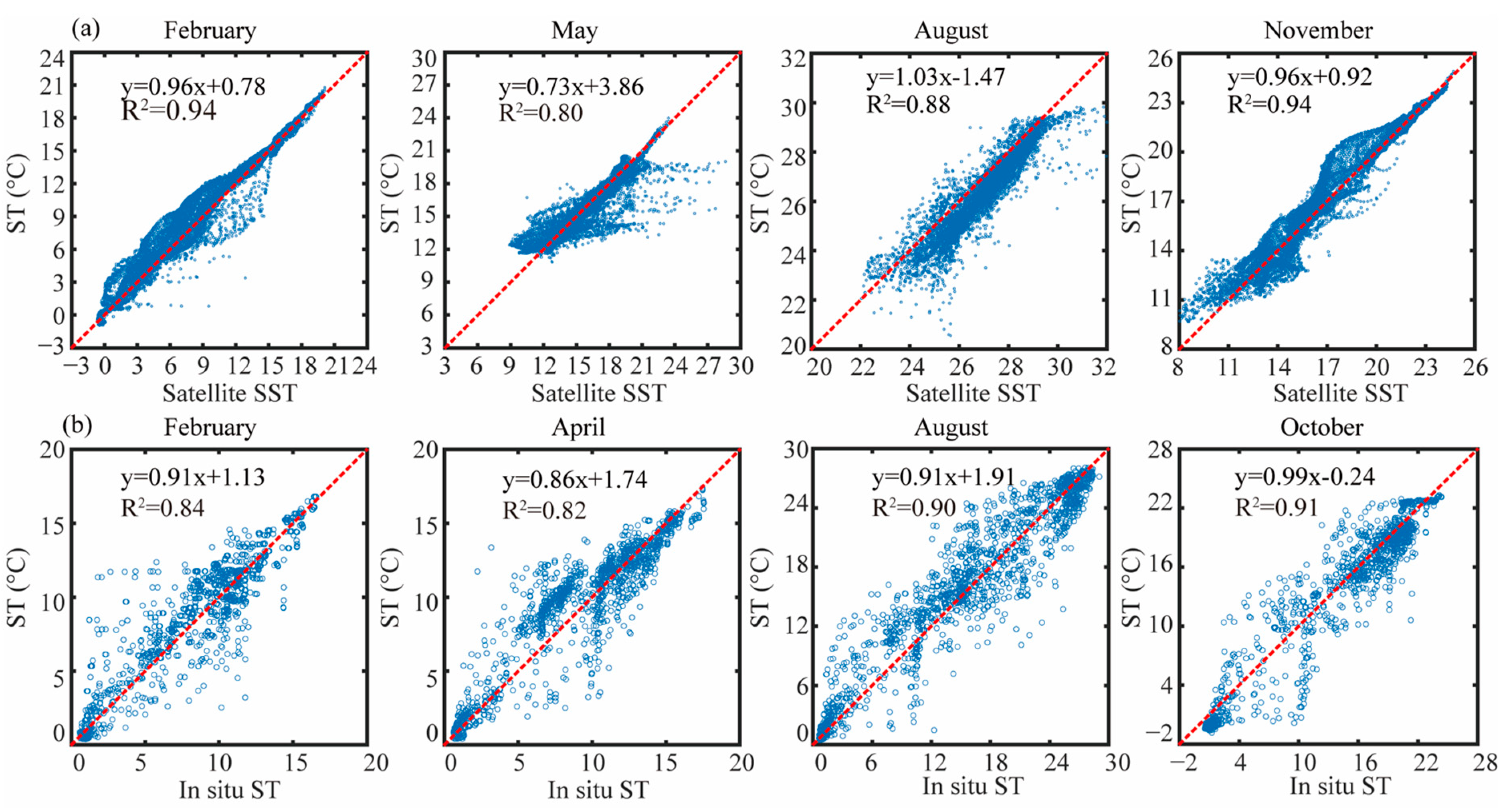
2.2.1. Verification of Seawater Temperature Data from GLORYS

To verify the accuracy of the ST from GLORYS, the surface and vertical profile data were matched with the satellite SST data from MODIS-Aqua and the in situ data from KODC, respectively (Figure 2). Details of the data matchup process were described by Stepanova et al. [35]. Briefly, a time window of ±30 days was used between the two datasets (in situ and satellite data) and the ST from GLORYS, and a median value from a 3 × 3-pixel box centered at each sampling site was applied to filter the sensor and algorithm noise. Finally, only the matrix with a coefficient of variability less than 0.4 was retained, and the average value of the matrix was calculated; this represented the matched data for the ST from GLORYS. Figure 2 shows that the ST from GLORYS fitted well with the satellite SST and in situ data from KODC, and the coefficient of determination was consistent with the results obtained by Stepanova et al. [36] (R² > 0.80). Therefore, the ST from GLORYS was used to explore the horizontal and vertical distributions of the ST in the YS, thereby providing important support analyses of the spatial and temporal distributions of the YSCWM [37].

2.2.2. Wavelet Analysis

The continuous wavelet transform (CWT) was used to determine the oscillation periods for the characteristic parameters of the YSCWM on the interannual scale. The CWT decomposed non-stationary time series into a time–frequency space, analyzed the local variability in energy, and translated the mother wavelet [38]. The MWC extracts various multivariate relationships in geology, and it was used to identify scale-dependent relationships [39]. Tests based on artificial datasets showed that MWC has advantages compared with other multivariable methods (i.e., multispectral coherence and multivariable empirical mode decomposition) when identifying multivariable relationships between scale correlation and localization. The MWC at the 95% confidence level was calculated using the Monte Carlo method [40]. The MWC can extend wavelet coherence from two variables to multiple variables. Given a predictor variable set X (X = [X₁, X₂, …, X_q]) and a response variable Y, the MWC was defined as follows [38,39,40]:

$${\mathsf{\rho }}_{\mathrm{m}}^2\left(\mathrm{s}, \mathsf{\tau }\right)=\frac{{\underset{\mathrm{W}}{\leftrightarrow }}^{\mathrm{Y}, \mathrm{X}}(\mathrm{s}, \mathsf{\tau }){\underset{\mathrm{W}}{\leftrightarrow }}^{\mathrm{X}, \mathrm{X}}{(\mathrm{s}, \mathsf{\tau })}^{-1}{\underset{\mathrm{W}}{\leftrightarrow }}^{\mathrm{Y}, \mathrm{X}}{(\mathrm{s}, \mathsf{\tau })}^{*}}{{\underset{\mathrm{W}}{\leftrightarrow }}^{\mathrm{Y}, \mathrm{Y}}(\mathrm{s}, \mathsf{\tau })}$$

(1)

where ${\underset{\mathrm{W}}{\leftrightarrow }}^{\mathrm{Y}, \mathrm{X}}(\mathrm{s},\mathsf{\tau })$ is the smoothed cross-wavelet power spectra between Y and X; ${\underset{\mathrm{W}}{\leftrightarrow }}^{\mathrm{X}, \mathrm{X}}(\mathrm{s},\mathsf{\tau })$ is the smoothed auto- and cross-wavelet power spectra among X; ${\underset{\mathrm{W}}{\leftrightarrow }}^{\mathrm{Y}, \mathrm{Y}}(\mathrm{s},\mathsf{\tau })$ is the smoothed wavelet power spectrum of Y; and ${\underset{\mathrm{W}}{\leftrightarrow }}^{\mathrm{Y}, \mathrm{X}}{(s,\tau )}^{\mathrm{*}}$ is the complex conjugate of ${\underset{\mathrm{W}}{\leftrightarrow }}^{\mathrm{Y}, \mathrm{X}}(\mathrm{s},\mathsf{\tau })$. In this study, the performance of one-, two-, three- and four-factor combinations when explaining the YSCWM intensity variability at all periods was assessed by the coherence and percent area of significant coherence (PASC) using MWC, as developed by Hu et al. [39]. Statistically, an increase in PASC indicates that a significant increase in variability can be explained at a 95% significance level. In practice, an additional factor is considered significant when it results in a ≥5% increase in PASC. Greater coherence with a larger PASC indicates that environmental variables can explain more variation. The MATLAB codes and user manual document for calculating the MWC and significance level are provided in the supplementary files of Hu et al. [39].

3. Results

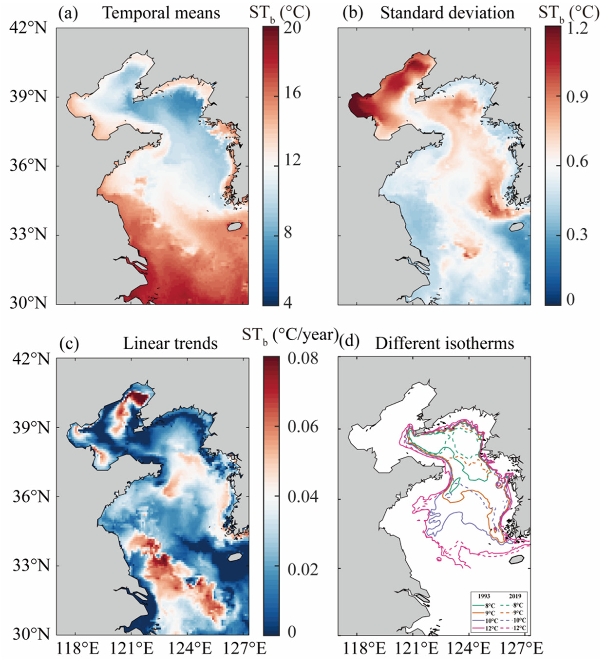
3.1. Spatial Patterns of Annual and Interannual Seawater Temperature in the Bottom Layer of the YS

The spatial distribution of the ST_b in the YS averaged from 1993–2019 is shown in Figure 3a. Spatially, the ST_b gradually decreased from the inshore to the center of the YS, with a mean value of 13.03 °C. The minimum (3.45 °C) occurred in the northern YS and the maximum (19.31 °C) occurred in the inshore water. The standard deviation of the detrended annual ST_b exhibited stronger interannual variability in the YSCWM than in surrounding waters (Figure 3b). On the interannual scale, the enclosure area surrounded by each isotherm shrank in the YSCWM. In particular, the enclosure area surrounded by isotherms at 10 °C shrank the most rapidly, followed by those at 9 °C and 8 °C, and shrank most slowly at 12 °C (Figure 3d). In addition, we fitted a linear function to the ST_b and calculated the linear trends. The interannual variability of the ST_b was stronger in the NYSCWM than in the SYSCWM (Figure 3c). The results show that the annual warming trend was stronger in the SYSCWM than in the NYSCWM, which were converse with the pattern of annual ST_b, probably due to the differences in the physical oceanographic conditions between the NYSCWM and SYSCWM, as discussed in Section 4.2.

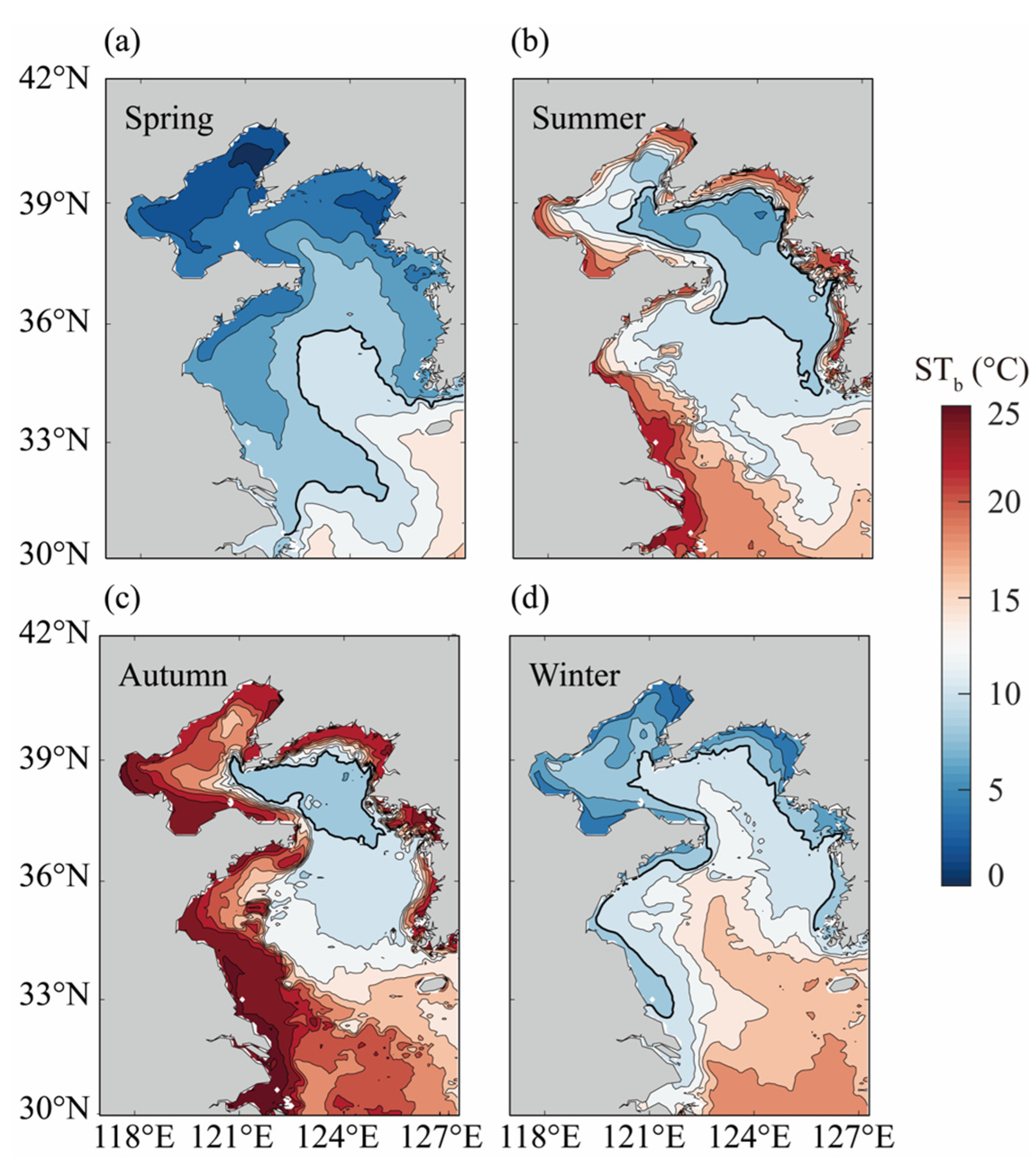
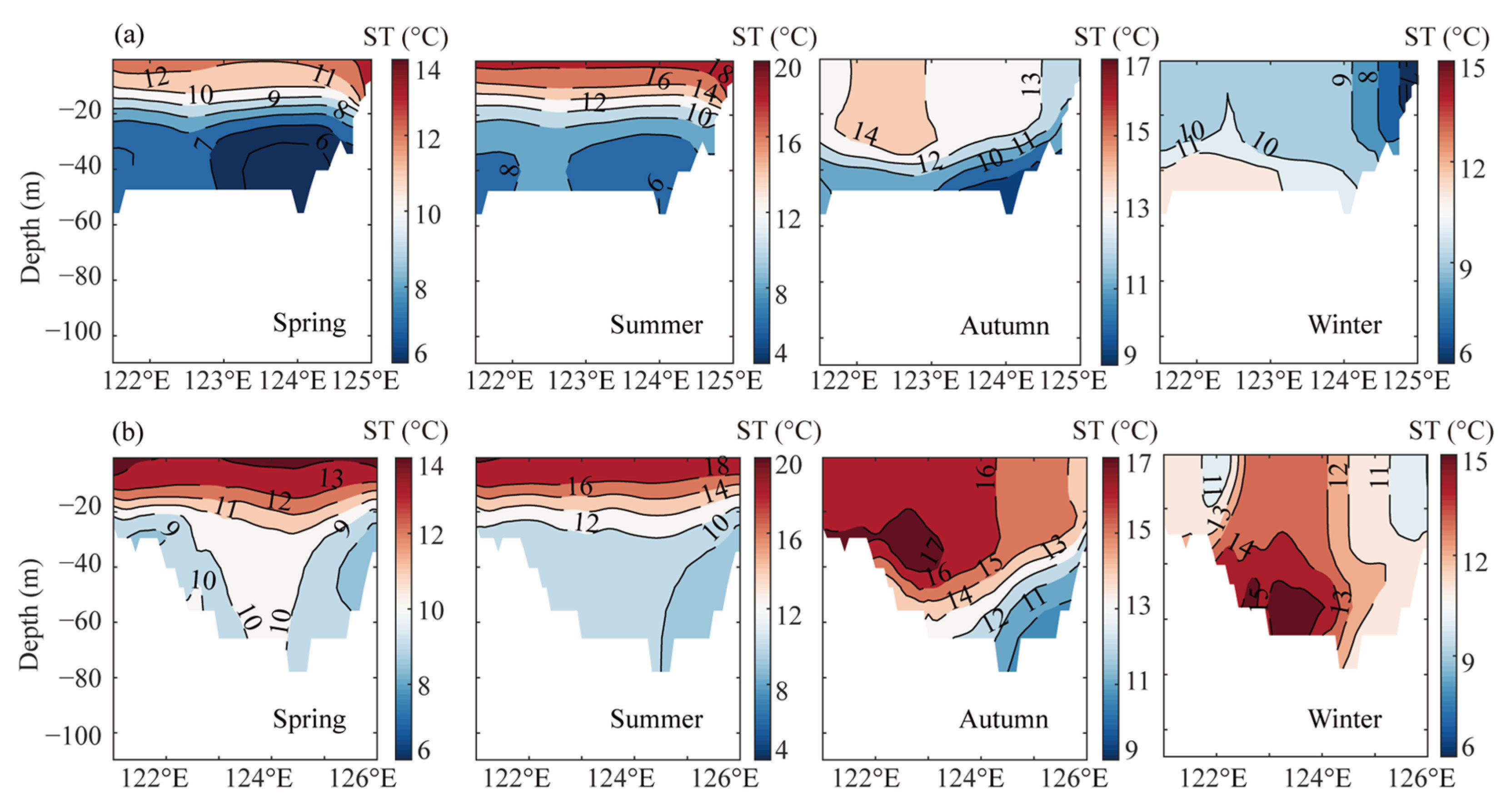
3.2. Seasonal Formation and Evolution of the YSCWM

The monthly ST_b in YS was analyzed to study the formation and evolution of the YSCWM from 1993 to 2019. In winter, the ST_b in the central region of the YS was higher than that in the surrounding regions (Figure 4a). In Spring, the YS started to warm up but the ST_b in the central region of the YS was lower compared with the surrounding regions. This cold ST_b was accompanied by the formation of closed isotherms in the bottom layer of the YS, which indicated the formation of the YSCWM (Figure 4b). In summer, the enclosure area of the YSCWM in the 10 °C isotherm range increased further and the 10 °C isotherm marked its core range, covering most of the YS and extending to its southern boundary at 34° N. A strong ST_b front formed in the surrounding seawater (Figure 4c). In autumn, the cold air from the north strengthened and gradually moved southward, thereby resulting in a gradual increase in the ST_b. The enclosure area of the YSCWM shrank, indicating a gradual decrease in its intensity (Figure 4d).

The 38.667° N and 36° N sections spanned the centers of the NYSCWM and SYSCWM, respectively, so they were selected to explore further the mechanisms responsible for the formation and evolution of the YSCWM. In the 38.667° N section (Figure 5a), the vertical structure of the ST was in a uniform state in the previous winter. In spring, the vertical distribution of the ST had an apparent three-layered structure, where the upper layer was warm and mixed, the middle layer was the thermocline with a sharp ST gradient of 0.5–1 °C/m, and the lower layer was uniform. This structure indicated the start of NYSCWM formation because a region with an ST_b lower than 10 °C appeared (Figure 4b). In summer, the thermocline intensified significantly, where the ST gradient of the central zone was 1 °C/m or more. The NYSCWM was completely mature during this time. In autumn, the upper boundary of the thermocline sank, and it was only present in the deepwater region below 30 m. The NYSCWM started to disappear during this period.

In the 36° N section, the evolution processes of the thermoclines in the SYSCWM were similar to the NYSCWM, but their vertical structures differed due to factors such as the geographical location, topography, and tidal mixing intensity (Figure 5b). In the previous winter, the ST_b in the central region of the SYSCWM was greater than 10 °C, and the ST in the central region was higher than that in coastal regions in the 36° N section. In spring, the ST_b of the SYSCWM had two cold centers on both flanks of the central trough, which suggested that the SYSCWM had a more complex structure in the spring than the NYSCWM. In summer, the two cold centers of the SYSCWM were completely merged, which indicated the peak of the SYSCWM. In autumn, the thermocline was only present in the central deepwater region below 40 m, and its intensity decreased significantly. The SYSCWM began to disappear during this period.

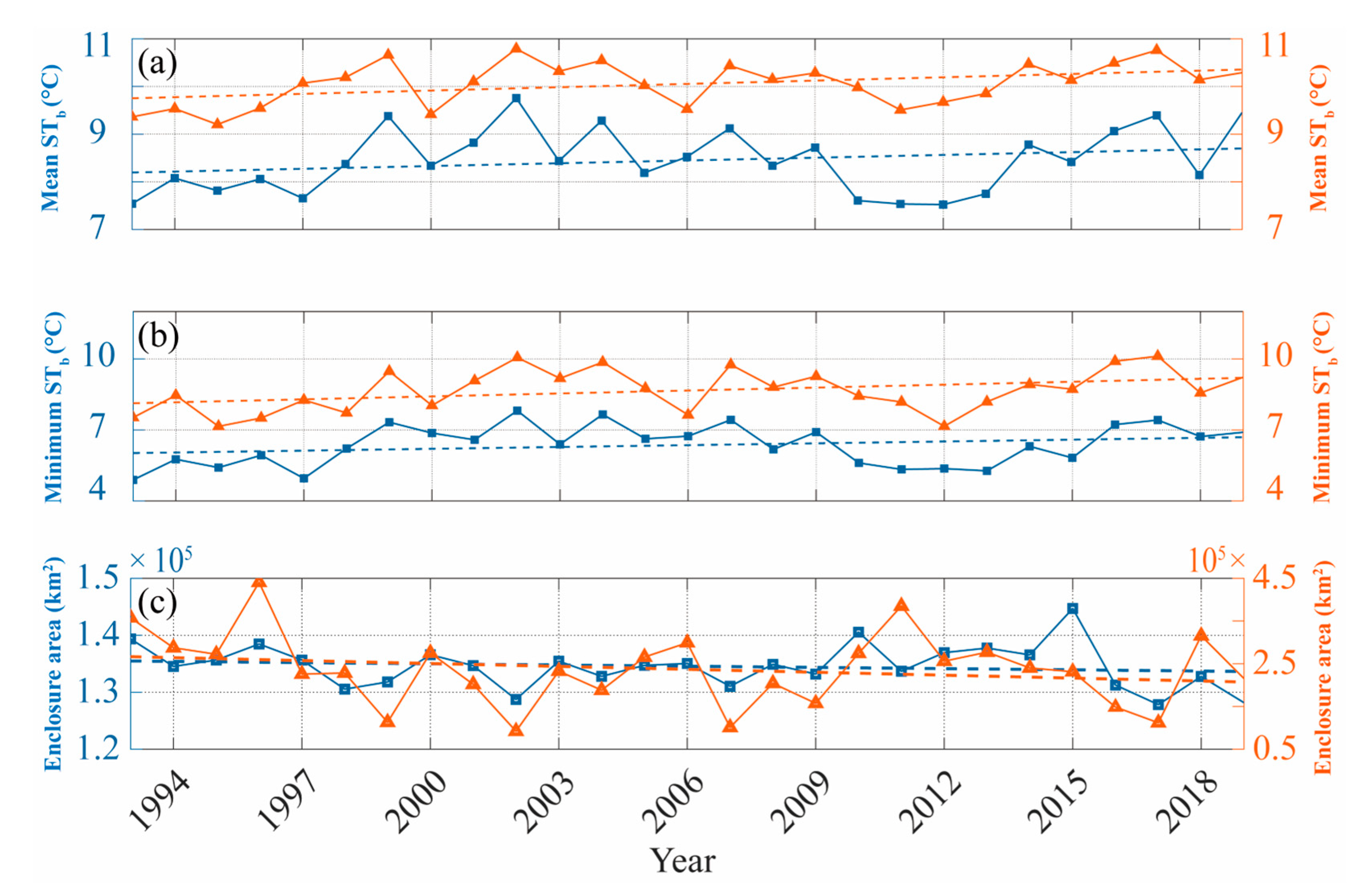
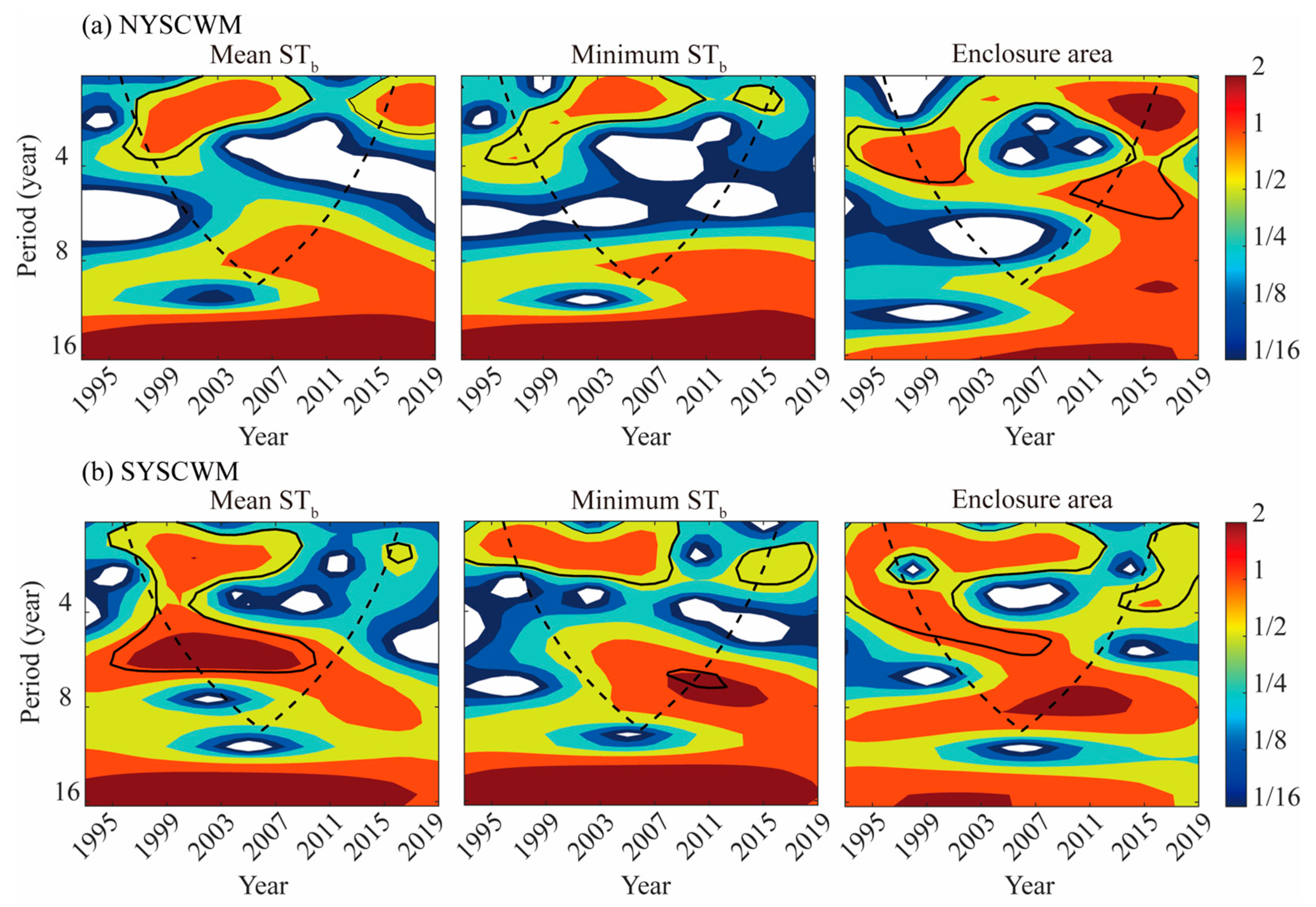
3.3. Interannual Variability of the YSCWM in the YS

The interannual variability in the YSCWM refers to fluctuations in the ST_b and area of the YSCWM over multiple years. The mean ST_b, minimum ST_b, and enclosure area were calculated to analyze the interannual variability in the intensities of the NYSCWM and SYSCWM. The correlation coefficients for the mean ST_b, minimum ST_b, and enclosure area between the NYSCWM and SYSCWM were 0.78, 0.77, and 0.56, respectively. The correlation coefficients of the three characteristic parameters of the NYSCWM and SYSCWM indicated that the variability in the three characteristic parameters was relatively consistent on the interannual scale (Figure 6). The standard deviation of the mean ST_b in the NYSCWM was 0.67, which was larger than that in the SYSCWM. The standard deviations of the minimum ST_b and enclosure area in the SYSCWM were larger than those in the NYSCWM, thereby indicating that the minimum ST_b and enclosure area of the SYSCWM changed more on the interannual scale. The highest mean ST_b value of the NYSCWM occurred in 2002 at 9.75 °C and the lowest occurred in 2012 at 7.52 °C. The highest mean ST_b value of the SYSCWM occurred in 2012 at 10.79 °C and the lowest occurred in 1995 at 9.20 °C.

The CWT was used to determine the periods of the three characteristic parameters of the NYSCWM and SYSCWM on the interannual scale. For the NYSCWM, the mean ST_b had the strongest periodic signal of about 3 years, where it mainly appeared from 1995 to 2009. There was no obvious periodic signal for the minimum ST_b after 2011. The periodic signal in the enclosure area was a strong periodic signal for 2–6 years in the whole study period (Figure 7a). For the SYSCWM, the mean ST_b had a strong periodic signal of 2–6 years, which mainly appeared in 1995–2009. The minimum ST_b had a strong periodic signal for 2–3 years, but there was no periodic signal after 2009. The periodic signal in the enclosure area was discontinuous in 1993–2019, and there were 2–6 years of periodic signals in 1993–2011, but only 2–3 years after 2011 (Figure 7b).

4. Discussion

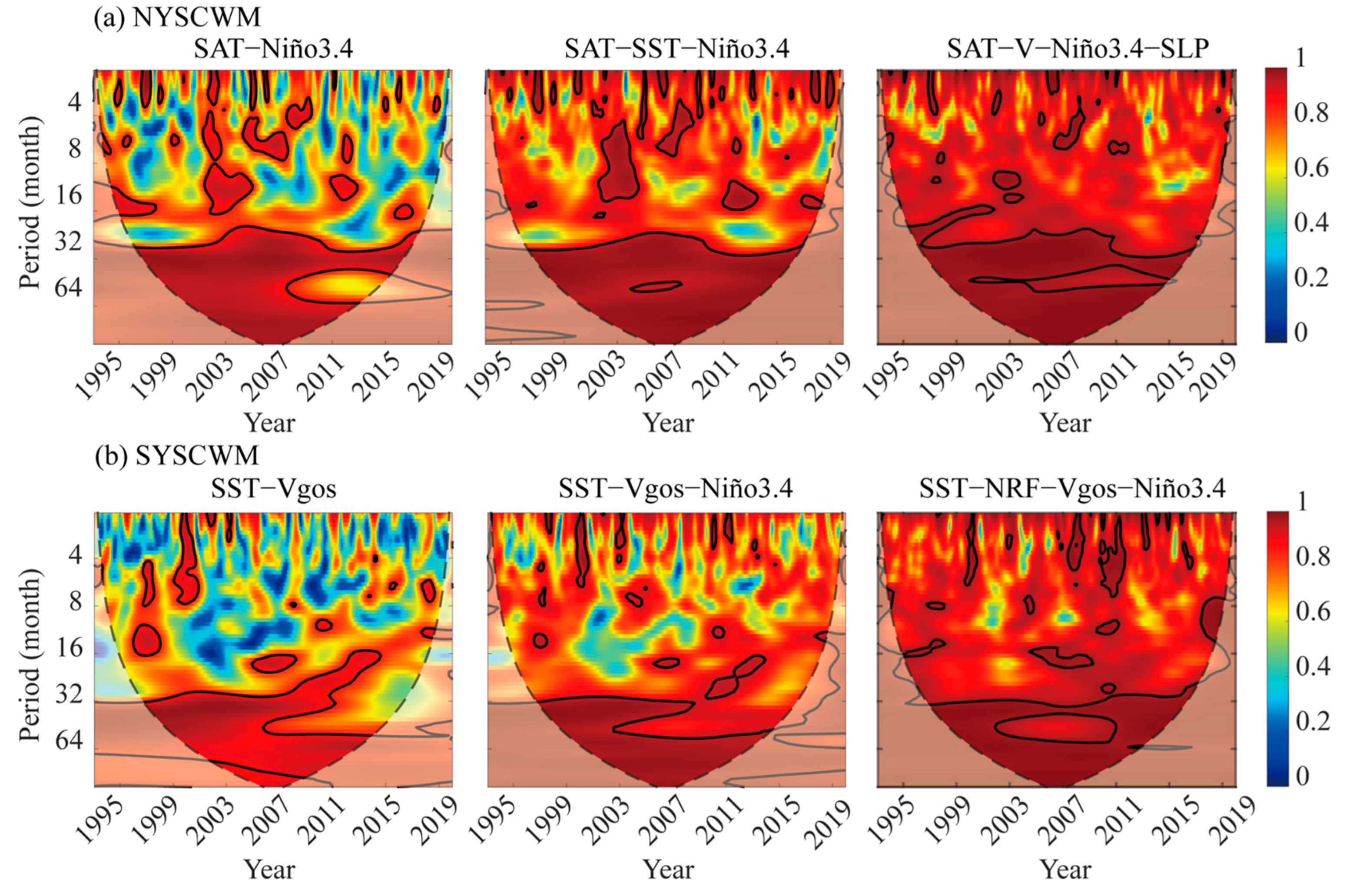
4.1. Combined Factors for Explaining Interannual Variability in Intensities of the NYSCWM and SYSCWM

Previous studies have shown that the intensity of the YSCWM is closely related to physical processes and environmental changes in the ocean [16,24]. Due to the minimum ST_b mainly representing the position change for the low ST center in the YSCWM [28], the mean ST_b was the most effective factor for characterizing the intensity of the YSCWM. The factors affecting the mean ST_b are complex, and the dominant factors differed with time in the NYSCWM and SYSCWM [41,42,43,44]. Thus, a de-seasoning analysis was first conducted for the mean ST_b and other physical environmental factors (V, U, SAT, NRF, SST, SLP, Vgos, and Ugos). Then, the MWC between the mean ST_b and every two or more factors was calculated to explore the main factors influencing the intensities of the NYSCWM and SYSCWM on the interannual scale. The coherence and the PASC of the best-combined factors are presented in

Table 2. Multivariate wavelet correlations between the mean ST_b and physical environmental factors in the NYSCWM and SYSCWM.

Combination	Region	Factor Combination	Coherence	PASC (%)
Two factors	NYSCWM	SAT–Niño 3.4	0.76	41.42
	SYSCWM	SST–Vgos	0.68	23.81
Three factors	NYSCWM	SAT–SST–Niño 3.4	0.87	41.69
	SYSCWM	SST–Vgos–Niño 3.4	0.83	28.91
Four factors	NYSCWM	SAT–V–Niño 3.4–SLP	0.93	41.92
	SYSCWM	SST–NRF–Vgos–Niño 3.4	0.92	37.80

. The PASC refers to the percent area of significant coherence relative to the entire wavelet time–scale domain [39]. Larger coherence and PASC values indicated that greater amounts of variability in the mean ST_b of the YSCWM could be explained by physical environmental factors (or combinations of factors) [45].

In this study, the calculation of the MWC between the mean ST_b and physical environmental factors (two-, three-, and four-factor) resulted in differences in the main factors influencing the variability in the intensity of the NYSCWM and SYSCWM (Figure 6). Table 2 summarizes the combinations of physical environmental factors (two, three, and four factors) that best explain the variability in the intensities of the NYSCWM and SYSCWM. For the NYSCWM, among all possible two-factor combinations, the SAT–Niño 3.4 combination was the best at explaining the variability in intensities at the 32–64-month time scale (about 3–5 years), and it was accompanied by an increase in the coherence and PASC (Table 2). These results indicate that the intensity variability was affected by the ENSO on the interannual scale (Figure 8). Many studies also detected an especially high mean ST_b and low enclosure area in ENSO years, as well as higher SAT and SST values and weaker winds in the YSCWM [21,31,46]. However, when the PASC increased as the coherence increased for the best combinations of three and four factors, the increases in the PASC were both <5%, thereby indicating that the additional factors were not considered significant or meaningful [47].

For the SYSCWM, SST–Vgos was the best two-factor combination for explaining the variability in intensity (Figure 8). Surface warming and the existence of the YSWC near the bottom layer together induced the increase in the mean ST_b of the SYSCWM [48]. When three factors were combined, the coherence of the SST–Vgos–Niño 3.4 combination explained 28.91% of the variability in the intensity of the SYSCWM [49]. Except for these factors, when NRF was added (four-factor combination), it could explain 37.80% of the variability in the intensity of the SYSCWM (Figure 8). The PASC of the SYSCWM increased by more than 5% (5.1% growth and 8.89% growth in three- and four-factor combinations, respectively), and this growth was considered significant, thereby indicating that additional factors could account for more variability in the intensity of the SYSCWM. These findings indicate that NRF and Niño 3.4 significantly influenced the variability in the intensity of the SYSCWM on the interannual scale [15,16,30].

4.2. Underlying Mechanisms Associated with Differences in Long-Term Trends in the Intensity of the NYSCWM and SYSCWM

One-dimensional linear trend analysis showed that the mean ST_b of the SYSCWM and NYSCWM exhibited upward warming trends of 0.024 °C/year and 0.018 °C/year (Figure 6a), and that the minimum ST_b had linear trends of 0.04 °C/year and 0.02 °C/year, respectively (Figure 6b). In addition, the enclosure area of the SYSCWM shrank at a higher rate (2193 km²/year) than that of the NYSCWM (67.78 km²/year). Since the mean ST_b and the minimum ST_b of the SYSCWM increased more each year, the enclosure area shrank more than that of the NYSCWM (Figure 6c). Thus, the intensity of the SYSCWM decreased more rapidly than that of the NYSCWM.

Horizontal heat transport was an important modifier of the thermal structure of the YSCWM during summer, and it could change the intensity of the YSCWM [16,30]. The surface currents could change the horizontal heat input into the YSCWM [50]. As surface currents circulate, they can transport warm water masses from one region to another. Previous studies, through numerical models and observations, have suggested that the summer circulation in the central part of the YS is cyclonic; thus, the wind and tidal forces may be major factors driving circulation in the YS [51,52,53,54]. According to the analysis of the mean geostrophic current in the summer, the dominant current was southward in the western half of the YS and northward in the eastern half. The northward current brought more warm water from the southern part of the YS, which increased the mean ST_b and the minimum ST_b, and shrank the enclosure area of the YSCWM to some extent (Figure 9a).

The NYSCWM and SYSCWM formed a counterclockwise cold water mass circulation [55,56]. In the 38.667° N section, the linear trend in the mean Ugos of the NYSCWM was negative in the eastern region and positive in the western region, which meant that the northward current was weakened and the southward current was similarly weakened (Figure 9c). However, in the 36° N section, the linear trend in the mean Ugos of the SYSCWM on both sides was opposite to that in the NYSCWM (Figure 9d). These findings indicated that the circulation was enhanced in the SYSCWM but weakened in the NYSCWM. The enhanced circulation in the SYSCWM could bring more surface warm water to its bottom core region. In addition, the northward winds accelerated horizontal heat transport in the SYSCWM to strengthen the warming process in the SYSCWM further (Figure 9b). In contrast, the weakening of the circulation in the NYSCWM led to less warm water intrusion being able to decrease the horizontal heat input. Therefore, the warming was more significant in the SYSCWM than in the NYSCWM, and thus, the increases in the mean ST_b and the minimum ST_b, and the shrink in the enclosure area of the SYSCWM, were more obvious compared with those in the NYSCWM from 1993 to 2019. The vertical velocity variability in currents can greatly influence various hydrological conditions by inducing or suppressing mixing [57]. The interactions between the YSCWM and the ambient hydrodynamic system could be further investigated through theoretical analysis in the future.

In addition to the effects of the circulation, the thermocline could also affect the differences in the chemical and hydrographic characteristics between the NYSCWM and SYSCWM [22,58]. The thermocline affects the YSCWM by regulating vertical stratification and stability. A stronger or deeper thermocline can impede vertical mixing between water layers, leading to more distinct water masses with varying temperatures and salinities. This thermocline variation, in turn, can influence the density gradients that drive current patterns in the YS [59]. We calculated the linear trends in the ST along the 38.667° N section and 36° N section in August (Figure 10a,b). The trend in the surface ST of the NYSCWM and SYSCWM both increased at the rate of 0.1 °C/decade and 0.2 °C/decade at a 95% significance level, and its correlation coefficient with ST_b was −0.68 and −0.64 in the NYSCWM and SYSCWM. Lateral heat input in the bottom layer weakened. The increasing trend in the SST and less warm water intrusion intensified the thermocline. Further, we calculated the vertical temperature gradient. The average vertical gradients with a water depth of 20–30 m above the NYSCWM and SYSCWM were regarded as the thermocline intensities [31]. The linear trends in the thermocline intensities increased at a rate of 0.004 °C/m/year in the NYSCWM and decreased at a rate of −0.003 °C/m/year in the SYSCWM at a 95% significance level, which meant that the amplitude of variation in the thermocline depth of the NYSCWM was stronger than that in the SYSCWM, especially after 2009 (Figure 10c). The correlation coefficient of the amplitude of variation in the thermocline depth and ST_b was −0.64 and −0.54 in the NYSCWM and SYSCWM. A stronger thermocline generated less vertical heat exchange across it. Less warm water intrusion reduced the horizontal heat input. This may have resulted from the weakening of the circulation in the NYSCWM in summer. An increasing surface ST and less bottom-layer horizontal heat input enhanced the seawater temperature difference between the surface and bottom layer. The stronger thermocline in the NYSCWM inhibited vertical heat exchange, which weakened the transfer of heat from the surface to the deep layer, thus weakening the ST_b during NYSCWM warming in summer. Therefore, the intensity of the SYSCWM decreased more rapidly than that of the NYSCWM.

5. Conclusions

The evolution and intensity of the YSCWM have a significant influence on the nutrient concentrations, primary production, and migration of fish in surrounding seawater. Therefore, knowing the variability in the intensity of the YSCWM at different scales in advance provides an important reference for a deeper understanding of the influence of hydrological processes on marine ecosystems in marginal seas. This study compared the difference in the interannual variability and long-term trends between the NYSCWM and SYSCWM, and explored the underlying mechanisms associated with differences in the long-term trends in the intensities of the NYSCWM and SYSCWM.

On the interannual scale, the mean ST_b, minimum ST_b, and enclosure area of the NYSCWM and SYSCWM exhibited consistent interannual variability, but the mean ST_b of the NYSCWM had a larger standard deviation and shorter periodic signal than that of the SYSCWM. The two-factor combinations of SAT–Niño 3.4 and SST–Vgos controlled the interannual variability in the intensities of the NYSCWM and SYSCWM, respectively. Moreover, the NRF and Niño 3.4 were still meaningful for explaining the intensity variability in the SYSCWM, which meant that the factors affecting the intensity variability of the NYSCWM and SYSCWM are different.

According to the analysis of the long-term trends, the increases in the mean ST_b and the minimum ST_b, and the shrinking of the enclosure area in the SYSCWM, were higher than those in the NYSCWM, and thus the intensity of the SYSCWM decreased more rapidly than that of the NYSCWM. Different thermocline and circulation feature intensities are the main reasons that different long-term trends in the intensity of the SYSCWM and NYSCWM are induced. Less warm water intrusion reduces the horizontal heat input, which results from the weakening of the circulation in the NYSCWM in summer. An increasing surface ST and less bottom-layer horizontal heat input enhance the seawater temperature difference between the surface and bottom layer. The stronger thermocline in the NYSCWM inhibits vertical heat exchange, which weakens the transfer of heat from the surface to the deep layer, thus weakening the ST_b during NYSCWM warming in summer. In the future, we will aim to explore the specific physical processes through which mesoscale features impact the generation and evolution of the YSCWM. This may provide a more comprehensive understanding of the interplay between mesoscale variability and cold water mass dynamics.

References

1. Smith, K.L., Jr.; Ruhl, H.A.; Bett, B.J.; Billett, D.S.; Lampitt, M.; R.S.; Kaufmann, R.S. Climate, carbon cycling, and deep-ocean ecosystems. Proc. Natl. Acad. Sci. USA 2009, 106, 19211–19218. [Google Scholar] [CrossRef] [PubMed]
2. Brown, J.; Hill, A.; Fernand, L.E.; Horsburgh, K.J. Observations of a seasonal jet-like circulation at the central North Sea cold pool margin. Estuar. Coast. Shelf Sci. 1999, 48, 343–355. [Google Scholar] [CrossRef]
3. Horsburgh, K.J.; Hill, A.E.; Brown, J.; Fernand, L.; Garvine, R.W.; Angelico, M.M.P. Seasonal evolution of the cold pool gyre in the western Irish Sea. Prog. Oceanogr. 2000, 46, 1–58. [Google Scholar] [CrossRef]
4. Hill, A.E.; Durazo, R.; Smeed, D.A. Observations of a cyclonic gyre in the western Irish Sea. Cont. Shelf Res. 1994, 14, 479–490. [Google Scholar] [CrossRef]
5. Houghton, R.W.; Schlitz, R.; Beardsley, R.C.; Butman, B.; Chamberlin, J.L. The Middle Atlantic Bight Cold Pool: Evolution of the Temperature Structure During Summer 1979. J. Phys. Oceanogr. 1982, 12, 1019–1029. [Google Scholar] [CrossRef]
6. Warrach, K. Modelling the thermal stratification in the North Sea. J. Mar. Syst. 1998, 14, 151–165. [Google Scholar] [CrossRef]
7. Luyten, P.J.; Jones, J.E.; Proctor, R. A numerical study of the long- and short-term temperature variability and thermal circulation in the North Sea. J. Phys. Oceanogr. 2003, 33, 37–56. [Google Scholar] [CrossRef]
8. Yuan, D.L.; Li, Y.; Qiao, F.L.; Zhao, W. Temperature inversion in the Huanghai Sea bottom cold water in summer. Acta Oceanol. Sin. 2013, 32, 42–47. [Google Scholar] [CrossRef]
9. Wei, H.; Shi, J.; Lu, Y.Y.; Peng, Y.A. Interannual and long-term hydrographic changes in the Yellow Sea during 1977–1998. Deep-Sea Res. Part II-Top. Stud. Oceanogr. 2010, 57, 1025–1034. [Google Scholar] [CrossRef]
10. Yu, X.J.; Guo, X.Y.; Takeoka, H. Fortnightly Variation in the Bottom Thermal Front and Associated Circulation in a Semienclosed Sea. J. Phys. Oceanogr. 2016, 46, 159–177. [Google Scholar] [CrossRef]
11. Wei, Q.S.; Wang, B.; Fu, M.; Sun, J.; Yao, Q.; Xin, M.; Yu, Z. Spatiotemporal variability of physical-biogeochemical processes and intrinsic correlations in the semi-enclosed South Yellow Sea. Acta Oceanol. Sin. 2020, 39, 11–26. [Google Scholar] [CrossRef]
12. Du, B. The characteristics of cold water mass variation at the bottom of the North Yellow Sea and its hydrological effects on the mortality of shellfish cultured in the waters of outer Changshun Islands. Mar. Sci. Bull. 1996, 15, 17–28. [Google Scholar]
13. Li, W.J.; Wang, Z.; Huang, H. Relationship between the southern Yellow Sea Cold Water Mass and the distribution and composition of suspended particulate matter in summer and autumn seasons. J. Sea Res. 2019, 154, 101812. [Google Scholar] [CrossRef]
14. Guo, C.C.; Zhang, G.; Sun, J.; Leng, X.; Xu, W.; Wu, C.; Li, X.; Pujari, L. Seasonal responses of nutrient to hydrology and biology in the southern Yellow Sea. Cont. Shelf Res. 2020, 206, 104207. [Google Scholar] [CrossRef]
15. Park, S.; Chu, P.C.; Lee, J.H. Interannual-to-interdecadal variability of the Yellow Sea Cold Water Mass in 1967-2008: Characteristics and seasonal forcings. J. Mar. Syst. 2011, 87, 177–193. [Google Scholar] [CrossRef]
16. Zhu, J.Y.; Shi, J.; Guo, X.; Gao, H.; Yao, X. Air-sea heat flux control on the Yellow Sea Cold Water Mass intensity and implications for its prediction. Cont. Shelf Res. 2018, 152, 14–26. [Google Scholar] [CrossRef]
17. Zhai, F.G.; Liu, Z.; Li, P.; Gu, Y.; Hu, L.; Sun, L.; Yang, B. Monthly and Interannual Variations in Winter Positive Surface-Bottom Temperature Difference in Northeastern Coastal Waters of the Shandong Peninsula in the Yellow Sea. J. Geophys. Res.-Ocean. 2021, 126, e2021JC017562. [Google Scholar] [CrossRef]
18. Hao, J.J.; Chen, Y.L.; Wang, F.; Lin, P.F. Seasonal thermocline in the China Seas and northwestern Pacific Ocean. J. Geophys. Res.-Ocean. 2012, 117, C02022. [Google Scholar] [CrossRef]
19. Zhang, S.W.; Wang, Q.Y.; Lu, Y.; Cui, H.; Yuan, Y.L. Observation of the seasonal evolution of the Yellow Sea Cold Water Mass in 1996-1998. Cont. Shelf Res. 2008, 28, 442–457. [Google Scholar] [CrossRef]
20. He, C.B.; Wang, Y.; Lei, Z.; Xu, S.G. A preliminary study of the formation and its properties of the Yellow Sea Cold Water Mass. Oceanol. Limnol. Sin. 1959, 2, 11–15. [Google Scholar]
21. Li, X.W.; Wang, X.; Chu, P.C.; Zhao, D. Low-frequency variability of the Yellow Sea Cold Water Mass identified from the China Coastal waters and adjacent seas reanalysis. Adv. Meteorol. 2015, 2015, 269859. [Google Scholar] [CrossRef]
22. Ren, H.J.; Zhan, J. A numerical study on the seasonal variability of the Yellow Sea cold water mass and the related dynamics. J. Hydrodyn. 2005, 20, 887–896. [Google Scholar] [CrossRef]
23. Jiang, B.J.; Bao, X.; Wu, D.; Xu, J. Interannual variation of temperature and salinity of northern Huanghai Sea Cold Water Mass and its probable cause. Acta Oceanol. Sin. 2007, 29, 1–10. [Google Scholar] [CrossRef]
24. Yu, F.; Zhang, Z.; Diao, X.; Guo, J.; Tang, Y. Analysis of evolution of the Huanghai Sea Cold Water Mass and its relationship with adjacent water masses. Acta Oceanol. Sin. 2006, 28, 26–34. [Google Scholar] [CrossRef]
25. Wang, B.D. Characteristics of variations and interrelations of biogenic elements in the Huanghai Sea Cold Water Mass. Acta Oceanol. Sin. 2000, 22, 47–54. [Google Scholar] [CrossRef]
26. Zhang, Y.; Yang, Y. Analyses of the variational characteristics of the north Huanghai Sea Cold Water Mass. Mar. Forecast. 1996, 13, 15–21. [Google Scholar]
27. Zhang, Y.; He, X. The annual variation and its fore-casting of the intensity of cold water mass of the western-north Yellow Sea in spring. J. Ocean. Univ. Qingdao 1989, 19, 275–283. [Google Scholar] [CrossRef]
28. Weng, X.C.; Zhang, Y.; Wang, C.; Zhang, Q. The variational characteristics of the Huanghai Sea (Yellow Sea) cold water mass. Oceanol. Limnol. Sin. 1989, 19, 119–131. [Google Scholar] [CrossRef]
29. Li, J.C.; Li, G.X.; Xu, J.S.; Dong, P.; Qiao, L.L.; Liu, S.D.; Sun, P.K.; Fan, Z.S. Seasonal evolution of the Yellow Sea Cold Water Mass and its interactions with ambient hydrodynamic system. J. Geophys. Res.-Ocean. 2016, 121, 6779–6792. [Google Scholar] [CrossRef]
30. Guo, Y.; Mo, D.; Hou, Y. Interannual to Interdecadal Variability of the Southern Yellow Sea Cold Water Mass and Establishment of “Forcing Mechanism Bridge”. J. Mar. Sci. Eng. 2021, 9, 1316. [Google Scholar] [CrossRef]
31. Li, A.; Yu, F.; Diao, X.; Si, G. Interannual variability of temperature of the northern Yellow Sea Cold Water Mass. Acta Oceanol. Sin. 2015, 37, 30–42. [Google Scholar]
32. Lellouche, J.-M.; Greiner, E.; Romain, B.-B.; Gilles, G.; Angelique, M.; Marie, D.; Clement, B.; Mathieu, H.; Olivier, L.G.; Charly, R.; et al. The Copernicus Global 1/12 degrees Oceanic and Sea Ice GLORYS12 Reanalysis. Front. Earth Sci. 2021, 9, 698876. [Google Scholar] [CrossRef]
33. Bonjean, F.; Lagerloef, G.S.E. Diagnostic model and analysis of the surface currents in the tropical Pacific Ocean. J. Phys. Oceanogr. 2002, 32, 2938–2954. [Google Scholar] [CrossRef]
34. O’Reilly, J.E.; Maritorena, S.; Mitchell, B.G.; Siegel, D.A.; Carder, K.L.; Garver, S.A.; Kahru, M.; McClain, C. Ocean color chlorophyll algorithms for SeaWiFS. J. Geophys. Res. Ocean. 1998, 103, 24937–24953. [Google Scholar] [CrossRef]
35. Martin, M.A.; Ghent, D.; Pires, A.C.; Göttsche, F.-M.; Cermak, J.; Remedios, J.J. Comprehensive in situ validation of five satellite land surface temperature data sets over multiple stations and years. Remote Sens. 2019, 11, 479. [Google Scholar] [CrossRef]
36. Stepanova, N.; Mizyuk, A. On the Applicability of CMEMS Reanalysis Data for Investigation of the Cold Intermediate Layer in the South-Eastern Part of the Baltic Sea. Pure Appl. Geophys. 2022, 179, 3481–3492. [Google Scholar] [CrossRef]
37. Salon, S.; Cossarini, G.; Bolzon, G.; Feudale, L.; Lazzari, P.; Teruzzi, A.; Solidoro, C.; Crise, A. Novel metrics based on Biogeochemical Argo data to improve the model uncertainty evaluation of the CMEMS Mediterranean marine ecosystem forecasts. Ocean Sci. 2019, 15, 997–1022. [Google Scholar] [CrossRef]
38. Torrence, C.; Compo, G.P. A practical guide to wavelet analysis. Bull. Am. Meteorol. Soc. 1998, 79, 61–78. [Google Scholar] [CrossRef]
39. Hu, W.; Si, B.C. Multiple wavelet coherence for untangling scale-specific and localized multivariate relationships in geosciences. Hydrol. Earth Syst. Sci. 2016, 20, 3183–3191. [Google Scholar] [CrossRef]
40. Grinsted, A.; Moore, J.C.; Jevrejeva, S. Application of the cross wavelet transform and wavelet coherence to geophysical time series. Nonlinear Process. Geophys. 2004, 11, 561–566. [Google Scholar] [CrossRef]
41. Huang, H.; Chen, X.; Lin, L. Evolution and mechnism of the Qingdao cold water mass. Oceanol. Limnol. Sin. 2019, 50, 1191–1200. [Google Scholar]
42. Oh, K.-H.; Lee, S.; Song, K.-M.; Lie, H.-J.; Kim, Y.-T. The temporal and spatial variability of the Yellow Sea Cold Water Mass in the southeastern Yellow Sea, 2009–2011. Acta Oceanol. Sin. 2013, 32, 1–10. [Google Scholar] [CrossRef]
43. Hu, D.; Wang, Q. Interannual variability of the southern Yellow Sea Cold Water Mass. Chin. J. Oceanol. Limnol. 2004, 22, 231–236. [Google Scholar]
44. Yao, Z.; Bao, X.; Li, N.; Li, X.; Wan, K.; Song, J. Seasonal Evolution of the Northern Yellow Sea Cold Water Mass. J. Ocean Univ. China 2012, 42, 9–15. [Google Scholar]
45. Lu, X.L.; Liu, C.; Niu, Y.; Yu, S. Long-term and regional variability of phytoplankton biomass and its physical oceanographic parameters in the Yellow Sea, China. Estuar. Coast. Shelf Sci. 2021, 260, 107497. [Google Scholar] [CrossRef]
46. Zhou, W.; Wang, X.; Zhou, T.; Li, C.; Chan, J. Interdecadal variability of the relationship between the East Asian winter monsoon and ENSO. Meteorol. Atmos. Phys. 2007, 98, 283–293. [Google Scholar] [CrossRef]
47. Hu, W.; Si, B.C.; Biswas, A.; Chau, H.W. Temporally stable patterns but seasonal dependent controls of soil water content: Evidence from wavelet analyses. Hydrol. Process. 2017, 31, 3697–3707. [Google Scholar] [CrossRef]
48. Yu, F.; Ren, Q.; Diao, X.; Wei, C.; Hu, Y. The Sandwich Structure of the Southern Yellow Sea Cold Water Mass and Yellow Sea Warm Current. Front. Mar. Sci. 2022, 8, 767850. [Google Scholar] [CrossRef]
49. Li, A.; Yu, F.; Si, G.; Wei, C. Long-term temperature variation of the Southern Yellow Sea Cold Water Mass from 1976 to 2006. Chin. J. Oceanol. Limnol. 2017, 35, 1032–1044. [Google Scholar] [CrossRef]
50. Cushman-Roisin, B.; Beckers, J.-M. Introduction to Geophysical Fluid Dynamics: Physical and Numerical Aspects; Academic Press: Cambridge, MA, USA, 2011. [Google Scholar]
51. Moon, J.H.; Hirose, N.; Yoon, J.H. Comparison of wind and tidal contributions to seasonal circulation of the Yellow Sea. J. Geophys. Res. Ocean. 2009, 114, C08016. [Google Scholar] [CrossRef]
52. Wang, B.; Hirose, N.; Moon, J.-H.; Yuan, D. Comparison of Tidal and Wind Contributions to Lagrangian Trajectories in the Southwestern Yellow Sea. Rep. Res. Inst. Appl. Mech. Kyushu Univ. 2012, 143, 43–48. [Google Scholar] [CrossRef]
53. Beardsley, R.C.; Limeburner, R.; Kim, K.; Candela, J. Lagrangian flow observations in the East China, Yellow and Japan seas. La Mer 1992, 30, 297–314. [Google Scholar]
54. Xia, C.S.; Qiao, F.L.; Yang, Y.Z.; Ma, J.; Yuan, Y.L. Three-dimensional structure of the summertime circulation in the Yellow Sea from a wave-tide-circulation coupled model. J. Geophys. Res.-Ocean. 2006, 111, C11S03. [Google Scholar] [CrossRef]
55. Zhao, B.R. A study of the circulations of the northern Yellow Sea cold water mass (NYSCWM)-Effects of tidal mixing on them. Oceanol. Limnol. Sin. 1996, 27, 429–435. [Google Scholar]
56. Song, D.H.; Bao, X.; Zhang, S.; Zhang, C. Three-dimensional numerical simulation of tides and tidal currents in Lianzhou Bay and adjacent areas. Mar. Sci. Bull. 2012, 31, 1–15. [Google Scholar] [CrossRef]
57. Black, W.J.; Dickey, T.D. Observations and analyses of upper ocean responses to tropical storms and hurricanes in the vicinity of Bermuda. J. Geophys. Res.-Ocean. 2008, 113, C08009. [Google Scholar] [CrossRef]
58. Xin, M.; Ma, D.; Wang, B. Chemicohydrographic characteristics of the Yellow Sea Cold Water Mass. Acta Oceanol. Sin. 2015, 34, 5–11. [Google Scholar] [CrossRef]
59. Alexander, M.A.; Scott, J.D.; Deser, C. Processes that influence sea surface temperature and ocean mixed layer depth variability in a coupled model. J. Geophys. Res.-Ocean. 2000, 105, 16823–16842. [Google Scholar] [CrossRef]
Figure 1. Bathymetry and schematic illustrations of regional circulation in the YS. The 38.667° N and 36° N sections are marked by the solid black lines. The boundary between the Northern Yellow Sea Cold Water Mass (NYSCWM) and Southern Yellow Sea Cold Water Mass (SYSCWM) is marked by the dashed black line. The circulation basically comprises the Yellow Sea Warm Current (YSWC), Yellow Sea Coastal Current (YSCC), Korean Coastal Current (KCC), Lubei Coastal Current (LBCC), Circulation of the NYSCWM (YC2), and Circulation of the SYSCWM (YC1).
Jmse 11 01888 g001
Figure 2. Verification of the ST data from GLORYS. (a) Correlation with the satellite SST from MODIS, (b) correlation with in situ data from KODC.
Jmse 11 01888 g002
Figure 3. Spatial patterns of STb in the YS from 1993 to 2019. (a) Temporal means, (b) standard deviations, (c) linear trends, (d) distribution of different isotherms. The solid lines in green, orange, purple, and pink represent the 1993 isotherms at 8 °C, 9 °C, 10 °C, and 12 °C, while the dotted lines in the same colors represent the 2019 isotherms at the same STb.
Jmse 11 01888 g003
Figure 4. Climatological seasonal mean STb in the YS. (a) Spring, (b) Summer, (c) Autumn, and (d) Winter. The interval of the thin black contour lines is 2 °C, and the 10 °C contour is the thick black line.
Jmse 11 01888 g004
Figure 5. Vertical structures of seasonal mean ST in sections. (a) 38.667° N section and (b) 36° N section.
Jmse 11 01888 g005
Figure 6. Interannual variability in the intensity of the YSCWM. (a) Mean STb, (b) minimum STb, and (c) enclosure area. The blue lines represent the characteristic parameters of the NYSCWM. The orange lines represent the characteristic parameters of the SYSCWM. The dotted lines represent the linear trend in the characteristic parameters of the NYSCWM and SYSCWM.
Jmse 11 01888 g006
Figure 7. Wavelet power spectrum for three characteristic parameters. (a) NYSCWM and (b) SYSCWM. The horizontal axis represents the study period. The solid line represents the 95% confidence test curve and the dotted line denotes the boundary not affected by the boundary effect of the wavelet transform. The white areas indicate that there were no significant frequency components or variations in the analyzed signal. The warm color indicates high power in an arbitrary unit, maintaining consistency with the unit of characteristic parameters determined using the CWT.
Jmse 11 01888 g007
Figure 8. Best two-, three-, and four-factor combinations for explaining the intensity of the (a) NYSCWM and (b) SYSCWM. The horizontal axis represents the study period. The solid line represents the 95% confidence test curve, the dotted line denotes the boundary not affected by the boundary effect of the wavelet transform, and the color denotes the strength of coherence.
Jmse 11 01888 g008
Figure 9. (a) Surface currents and (b) surface winds in summer (June–August). The linear trend in the mean Ugos, (c) 38.667° N section and (d) 36° N section, in 1993–2019.
Jmse 11 01888 g009
Figure 10. Linear trend diagram for (a) 38.667° N section and (b) 36° N section. The contour interval is 0.05 °C/decade. (c) The amplitude of variation in the thermocline for 20–30 m depth of YSCWM. The blue and orange lines represent the NYSCWM and SYSCWM, respectively.
Jmse 11 01888 g010