
Sustainable Maritime Transportation Operations with Emission Trading
Abstract
:1. Introduction
- 1.
- What are the optimal sailing speeds within the EU and non-EU areas that minimize the shipping company’s total costs under the new EU policy on emissions?
- 2.
- What is the optimal number of ships to be equipped in the shipping route that leads to the lowest total costs while adhering to the emissions reduction requirements set by the EU’s policy?
- 3.
- How do the optimal sailing speeds within EU and non-EU areas, as well as the optimal number of ships equipped in the shipping route, vary with changes in the charged fee for emissions, fuel price, and weekly operational costs of ships?
1.1. Literature Review
1.1.1. Carbon Emission Reduction Policies in Shipping
1.1.2. Optimal Decisions in Shipping
1.2. Research Contributions
- 1.
- Theoretical contributions. This study addresses a research gap, as existing literature has not focused on the optimal decisions of sailing speed and the number of ships under the newly proposed EU policy. To the best of our knowledge, this is the first study to establish mathematical models aimed at minimizing the total costs of shipping companies while considering the implications of the new EU policy. The proposed approach involves a nonlinear optimization model to determine the shipping company’s optimal decisions. By leveraging the unique structure of the optimization problem under the new EU policy, two propositions are proven. We further transform the nonlinear model into a solvable IP model. Through experiments and sensitivity analyses, specific solutions are obtained, and the impacts of different parameters are tested.
- 2.
- Practical contributions. This study contributes valuable insights into optimal strategies for shipping companies to minimize costs and comply with the new EU emissions policy. The results have practical implications for the sustainable development of the shipping industry and its adherence to environmental regulations. The proposed mathematical model can serve as a decision tool for shipping companies facing the new EU emissions policy.
2. Problem Description and Model Development
3. Solution Methods
4. Experiments
4.1. Experiment Settings
4.1.1. Selected Shipping Routes
4.1.2. Parameter Settings
- 1.
- The fixed cost c. Referring to [34], we first set c = 180,000 per week for a 5000-TEU (twenty-foot equivalent unit) container ship.
- 2.
- The fuel price . Referring to [35], we set to be an average value of 600 (USD/tonne).
- 3.
- The charged fee of emissions . EU ETS allowance prices closed at USD 102 per tonne on April 17, according to Ice Exchange data [7].
- 4.
- The conversion rate of fuel consumption and emissions is set to 3.15 [36].
- 5.
- Referring to [32], we set .
- 6.
- The berthing time at port i3: Busan—1.1 days; Ningbo—1.5 days; Shanghai—1.0 day; Yantian—0.6 day; Singapore—1.0 day; Algeciras—0.7 day; Dunkerque—1.6 days; Le Havre—0.8 day; Hamburg—1.4 days; Wilhelmshaven—1.1 days; Rotterdam—1.3 days; Tianji—1.2 days; Dalian—1.5 days; Qingdao—1.5 days; Antwerp—1.3 days.
- 7.
- We set the emissions per hour during the berthing to be 2 tonnes; i.e., .
- 8.
- We set knots and knots.
4.2. Basic Results
4.3. Sensitivity Analysis
4.3.1. Impact of the Charged Fee of Emissions
4.3.2. Impact of the Fuel Price
4.3.3. Impact of the Weekly Fixed Cost per Ship
5. Conclusions
Author Contributions
Funding
Institutional Review Board Statement
Informed Consent Statement
Data Availability Statement
Conflicts of Interest
| 1 | https://www.cma-cgm.com/products-services/flyers, accessed on 4 August 2023 |
| 2 | http://port.sol.com.cn/licheng.asp, accessed on 4 August 2023 |
| 3 | https://www.econdb.com/maritime/ports/, accessed on 5 August 2023 |
References
- Wang, S.; Yin, J.; Khan, R.U. Dynamic Safety Assessment and Enhancement of Port Operational Infrastructure Systems during the COVID-19 Era. J. Mar. Sci. Eng. 2023, 11, 1008. [Google Scholar] [CrossRef]
- Wu, Y.; Huang, Y.; Wang, H.; Zhen, L. Joint planning of fleet deployment, ship refueling, and speed optimization for dual-fuel ships considering methane slip. J. Mar. Sci. Eng. 2022, 10, 1690. [Google Scholar] [CrossRef]
- IMO. Fourth IMO Greenhouse Gas Study. 2020. Available online: https://www.imo.org/en/OurWork/Environment/Pages/Fourth-IMO-Greenhouse-GasStudy2020.aspx (accessed on 5 August 2023).
- Central People’s Government of the People’s Republic of China. Suggestions on Complete, Accurate and Comprehensive Implementation of the New Development Concept to Do a Good Job in the Work of Carbon Peak Carbon Neutrality. 2021. Available online: https://www.gov.cn/zhengce/2021-10/24/content_5644613.htm (accessed on 4 August 2023).
- The European Parliament. Revision of the Renewable Energy Directive: Fit for 55 Package. 2023. Available online: https://www.europarl.europa.eu/thinktank/en/document/EPRS_BRI(2021)698781#:~:text=The%20%27fit%20for%2055%27%20package%20is%20part%20of,EU%20deliver%20the%20new%2055%20%25%20GHG%20target (accessed on 4 August 2023).
- IMO. 2023 IMO Strategy on Reduction of GHG Emissions from Ships. 2023. Available online: https://www.imo.org/en/OurWork/Environment/Pages/2023-IMO-Strategy-on-Reduction-of-GHG-Emissions-from-Ships.aspx (accessed on 5 August 2023).
- Lloyd’s List. EU Parliament Approves Shipping’s Inclusion in Regional Carbon Market. 2023. Available online: https://lloydslist-maritimeintelligence-informa-com.ezproxy.lb.polyu.edu.hk/LL1144780/EU-Parliament-approves-shippings-inclusion-in-regional-carbon-market (accessed on 10 July 2023).
- Wu, M.; Li, K.X.; Xiao, Y.; Yuen, K.F. Carbon emission trading scheme in the shipping sector: Drivers, challenges, and impacts. Mar. Policy 2022, 138, 104989. [Google Scholar] [CrossRef]
- Zhu, M.; Shen, S.; Shi, W. Carbon emission allowance allocation based on a bi-level multi-objective model in maritime shipping. Ocean. Coast. Manag. 2023, 241, 106665. [Google Scholar] [CrossRef]
- Chang, C.C.; Huang, P.C. Carbon allowance allocation in the shipping industry under EEDI and non-EEDI. Sci. Total Environ. 2019, 678, 341–350. [Google Scholar] [CrossRef]
- Chen, S.; Zheng, S.; Sys, C. Policies focusing on market-based measures towards shipping decarbonization: Designs, impacts and avenues for future research. Transp. Policy 2023, 137, 109–124. [Google Scholar] [CrossRef]
- Gu, Y.; Wallace, S.W.; Wang, X. Can an Emission Trading Scheme really reduce CO2 emissions in the short term? Evidence from a maritime fleet composition and deployment model. Transp. Res. Part D Transp. Environ. 2019, 74, 318–338. [Google Scholar] [CrossRef]
- Heine, D.; Gäde, S. Unilaterally removing implicit subsidies for maritime fuels: A mechanism to unilaterally tax maritime emissions while satisfying extraterritoriality, tax competition and political constraints. Int. Econ. Econ. Policy 2018, 15, 523–545. [Google Scholar] [CrossRef]
- Tvedt, J.; Wergeland, T. Tax regimes, investment subsidies and the green transformation of the maritime industry. Transp. Res. Part D Transp. Environ. 2023, 119, 103741. [Google Scholar] [CrossRef]
- Merk, O.M. Quantifying tax subsidies to shipping. Marit. Econ. Logist. 2020, 22, 517–535. [Google Scholar] [CrossRef]
- Bouman, E.A.; Lindstad, E.; Rialland, A.I.; Strømman, A.H. State-of-the-art technologies, measures, and potential for reducing GHG emissions from shipping—A review. Transp. Res. Part D Transp. Environ. 2017, 52, 408–421. [Google Scholar] [CrossRef]
- Lin, D.Y.; Juan, C.J.; Ng, M. Evaluation of green strategies in maritime liner shipping using evolutionary game theory. J. Clean. Prod. 2021, 279, 123268. [Google Scholar] [CrossRef]
- Adland, R.; Cariou, P.; Jia, H.; Wolff, F.C. The energy efficiency effects of periodic ship hull cleaning. J. Clean. Prod. 2018, 178, 1–13. [Google Scholar] [CrossRef]
- European Parliament. Cutting Emissions from Planes and Ships: EU Actions Explained. 2023. Available online: https://www.europarl.europa.eu/news/en/headlines/society/20220610STO32720/cutting-emissions-from-planes-and-ships-eu-actions-explained (accessed on 5 August 2023).
- Panoutsou, C.; Germer, S.; Karka, P.; Papadokostantakis, S.; Kroyan, Y.; Wojcieszyk, M.; Maniatis, K.; Marchand, P.; Landalv, I. Advanced biofuels to decarbonise European transport by 2030: Markets, challenges, and policies that impact their successful market uptake. Energy Strategy Rev. 2021, 34, 100633. [Google Scholar] [CrossRef]
- Lin, D.-Y.; Tsai, Y.-Y. The ship routing and freight assignment problem for daily frequency operation of maritime liner shipping. Transp. Res. Part E Logist. Transp. Rev. 2014, 67, 52–70. [Google Scholar] [CrossRef]
- Lin, D.Y.; Chang, Y.T. Ship routing and freight assignment problem for liner shipping: Application to the Northern Sea Route planning problem. Transp. Res. Part E Logist. Transp. Rev. 2018, 110, 47–70. [Google Scholar] [CrossRef]
- Dai, W.L.; Fu, X.; Yip, T.L.; Hu, H.; Wang, K. Emission charge and liner shipping network configuration—An economic investigation of the Asia-Europe route. Transp. Res. Part A Policy Pract. 2018, 110, 291–305. [Google Scholar] [CrossRef]
- Zhen, L.; Hu, Y.; Wang, S.; Laporte, G.; Wu, Y. Fleet deployment and demand fulfillment for container shipping liners. Transp. Res. Part Methodol. 2019, 120, 15–32. [Google Scholar] [CrossRef]
- Zhao, Y.; Chen, Z.; Lim, A.; Zhang, Z. Vessel deployment with limited information: Distributionally robust chance constrained models. Transp. Res. Part B Methodol. 2022, 161, 197–217. [Google Scholar] [CrossRef]
- Wang, C.; Xu, C. Sailing speed optimization in voyage chartering ship considering different carbon emissions taxation. Comput. Ind. Eng. 2015, 89, 108–115. [Google Scholar] [CrossRef]
- Sheng, D.; Meng, Q.; Li, Z.C. Optimal vessel speed and fleet size for industrial shipping services under the emission control area regulation. Transp. Res. Part C Emerg. Technol. 2019, 105, 37–53. [Google Scholar] [CrossRef]
- Wang, H.; Wang, S.; Meng, Q. Simultaneous optimization of schedule coordination and cargo allocation for liner container shipping networks. Transp. Res. Part E Logist. Transp. Rev. 2014, 70, 261–273. [Google Scholar] [CrossRef]
- Koza, D.F. Liner shipping service scheduling and cargo allocation. Eur. J. Oper. Res. 2019, 275, 897–915. [Google Scholar] [CrossRef]
- Ozcan, S.; Eliiyi, D.T.; Reinhardt, L.B. Cargo allocation and vessel scheduling on liner shipping with synchronization of transshipments. Appl. Math. Model. 2020, 77, 235–252. [Google Scholar] [CrossRef]
- Giovannini, M.; Psaraftis, H.N. The profit maximizing liner shipping problem with flexible frequencies: Logistical and environmental considerations. Flex. Serv. Manuf. J. 2019, 31, 567–597. [Google Scholar] [CrossRef]
- Wang, S.; Meng, Q. Sailing speed optimization for container ships in a liner shipping network. Transp. Res. Part E Logist. Transp. Rev. 2012, 48, 701–714. [Google Scholar] [CrossRef]
- Wang, H.; Yan, R.; Au, M.H.; Wang, S.; Jin, Y.J. Federated learning for green shipping optimization and management. Adv. Eng. Inform. 2023, 56, 101994. [Google Scholar] [CrossRef]
- Wu, Y.; Huang, Y.; Wang, H.; Zhen, L.; Shao, W. Green Technology Adoption and Fleet Deployment for New and Aged Ships Considering Maritime Decarbonization. J. Mar. Sci. Eng. 2022, 11, 36. [Google Scholar] [CrossRef]
- ShipBunker. 2023. Available online: https://shipandbunker.com/prices (accessed on 28 July 2023).
- Offshore Energy. 2023. Available online: https://www.offshore-energy.biz/marine-benchmark-2020-global-shipping-co2-emissions-down-1/ (accessed on 28 July 2023).
- Drewry. COVID-19 Drives up Ship Operating Costs. 2020. Available online: https://www.drewry.co.uk/news/news/covid-19-drives-up-ship-operating-costs (accessed on 30 July 2023).


| Sets | |
|---|---|
| I | Set of ports of call in a shipping route, |
| Set of ports in the EU area, | |
| Set of ports outside the EU area, | |
| Set of the legs on which emissions are 0 charged, | |
| Set of the legs on which emissions are 50% charged, | |
| Set of the legs on which emissions are 100% charged, | |
| Parameters | |
| c | The fixed cost for each ship per week |
| The fuel price per tonne | |
| The charged fee of emissions per tonne | |
| The conversion rate of fuel consumption and emissions | |
| Q | The emission per hour during berthing |
| The distance of leg i | |
| The berthing time at port i | |
| The sailing speed on leg i | |
| The minimum sailing speed | |
| The maximum sailing speed | |
| X | The integer used to discretize sailing speed, |
| The discretized sailing speed, | |
| Function | |
| Fuel consumption at the sailing speed of | |
| Decision variables | |
| z | The number of deployed ships in a route |
| Binary decision variable that equals 1 if ships sail with speed and 0 otherwise |
| Route ID | Port Rotation (City) |
|---|---|
| 1 | Busan → Ningbo → Shanghai → Yantian → Singapore → Algeciras → Dunkerque → Le Havre → Hamburg → Wilhelmshaven → Rotterdam → Port Klang → Busan |
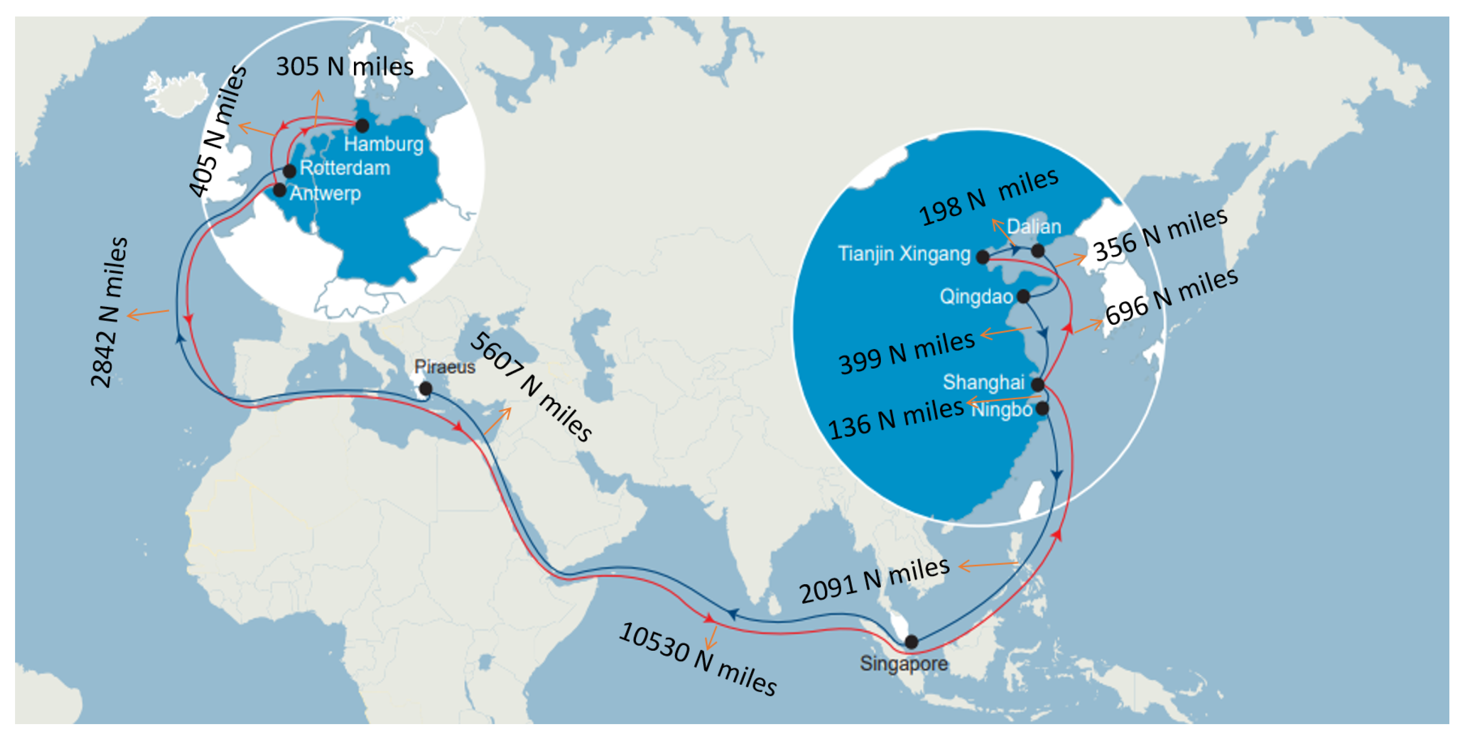
| 2 | Tianjin → Dalian → Qingdao → Shanghai → Ningbo → Singapore→ Piraeus → Rotterdam → Hamburg → Antwerp → Shanghai → Tianjin |
| Route ID | Set of Legs | Legs | Total Distance (Nautical Mile) | Sailing Speed (knot) | Number of Ships | OBJ (USD) |
|---|---|---|---|---|---|---|
| 1 | Busan → Ningbo → Shanghai → Yantian → Singapore; Port Klang → Busan | 3901 | 13.0 | 13 | 3,924,499.1 | |
| Singapore → Algeciras; Rotterdam → Port Klang | 15,020 | 12.1 | ||||
| Algeciras → Dunkerque → Le Havre → Hamburg → Wilhelmshaven → Rotterdam | 2269 | 11.6 | ||||
| 2 | Tianjin → Dalian → Qingdao → Shanghai → Ningbo → Singapore | 3876 | 12.8 | 14 | 4,166,763.3 | |
| Singapore→ Piraeus; Antwerp → Shanghai | 16,137 | 12.0 | ||||
| Piraeus→Rotterdam → Hamburg → Antwerp | 3552 | 11.1 |
| (USD/ton) | Set of Legs | Sailing Speed (knot) | Fuel Consumption (ton) | Number of Ships | OBJ (USD) |
|---|---|---|---|---|---|
| 80 | 12.8 | 0.90 | 14 | 4,101,154.6 | |
| 11.9 | 0.72 | ||||
| 11.5 | 0.65 | ||||
| 90 | 12.8 | 0.90 | 14 | 4,131,128.5 | |
| 12.0 | 0.74 | ||||
| 11.1 | 0.59 | ||||
| 100 | 12.8 | 0.90 | 14 | 4,160,824.1 | |
| 12.0 | 0.74 | ||||
| 11.1 | 0.59 | ||||
| 110 | 12.8 | 0.90 | 14 | 4,190,519.8 | |
| 12.0 | 0.74 | ||||
| 11.1 | 0.59 | ||||
| 120 | 13.3 | 1.01 | 14 | 4,220,180.5 | |
| 11.9 | 0.72 | ||||
| 11.1 | 0.59 | ||||
| 130 | 13.3 | 1.01 | 14 | 4,249,612.9 | |
| 11.9 | 0.72 | ||||
| 11.1 | 0.59 | ||||
| 140 | 13.3 | 1.01 | 14 | 4,279,045.4 | |
| 11.9 | 0.72 | ||||
| 11.1 | 0.59 | ||||
| 150 | 12.1 | 0.76 | 15 | 4,305,595.6 | |
| 11.1 | 0.59 | ||||
| 10.2 | 0.46 | ||||
| 160 | 12.1 | 0.76 | 15 | 4,331,828.7 | |
| 11.0 | 0.57 | ||||
| 10.2 | 0.46 | ||||
| 170 | 12.1 | 0.76 | 15 | 4,358,061.8 | |
| 11.0 | 0.57 | ||||
| 10.2 | 0.46 | ||||
| 180 | 12.1 | 0.76 | 15 | 4,384,294.9 | |
| 11.0 | 0.57 | ||||
| 10.2 | 0.46 |
| (USD/ton) | Set of Legs | Sailing Speed (knot) | Number of Ships | OBJ (USD) |
|---|---|---|---|---|
| 570 | 12.8 | 14 | 4,099,569.9 | |
| 12.0 | ||||
| 11.1 | ||||
| 580 | 12.8 | 14 | 4,121,967.7 | |
| 12.0 | ||||
| 11.1 | ||||
| 590 | 12.8 | 14 | 4,144,365.5 | |
| 12.0 | ||||
| 11.1 | ||||
| 600 | 12.8 | 14 | 4,166,763.3 | |
| 12.0 | ||||
| 11.1 | ||||
| 610 | 12.8 | 14 | 4,189,161.1 | |
| 12.0 | ||||
| 11.1 | ||||
| 620 | 12.8 | 14 | 4,211,558.85 | |
| 12.0 | ||||
| 11.1 | ||||
| 630 | 12.8 | 14 | 4,233,956.7 | |
| 12.0 | ||||
| 11.1 | ||||
| 640 | 12.8 | 14 | 4,256,354.4 | |
| 12.0 | ||||
| 11.1 | ||||
| 650 | 12.8 | 14 | 4,278,752.2 | |
| 12.0 | ||||
| 11.1 | ||||
| 660 | 12.1 | 15 | 4,300,885.9 | |
| 10.9 | ||||
| 10.6 | ||||
| 670 | 12.1 | 15 | 4,321,062.5 | |
| 10.9 | ||||
| 10.6 | ||||
| 680 | 12.1 | 15 | 4,341,239.1 | |
| 10.9 | ||||
| 10.6 | ||||
| 690 | 12.1 | 15 | 4,361,415.6 | |
| 10.9 | ||||
| 10.6 | ||||
| 700 | 12.1 | 15 | 4,381,592.2 | |
| 10.9 | ||||
| 10.6 |
| c (USD/week) | Set of Legs | Sailing Speed (knot) | Number of Ships | OBJ (USD) |
|---|---|---|---|---|
| 60,000 | 10.6 | 16 | 2,309,423.4 | |
| 10.2 | ||||
| 10.0 | ||||
| 80,000 | 10.6 | 16 | 2,629,423.4 | |
| 10.2 | ||||
| 10.0 | ||||
| 100,000 | 10.6 | 16 | 2,949,423.4 | |
| 10.2 | ||||
| 10.0 | ||||
| 120,000 | 10.6 | 16 | 3,269,423.4 | |
| 10.2 | ||||
| 10.0 | ||||
| 140,000 | 12.1 | 15 | 3,579,676.8 | |
| 11.0 | ||||
| 10.2 | ||||
| 160,000 | 12.1 | 15 | 3,879,676.8 | |
| 11.0 | ||||
| 10.2 | ||||
| 180,000 | 12.8 | 14 | 4,166,763.3 | |
| 12.0 | ||||
| 11.1 | ||||
| 200,000 | 12.8 | 14 | 4,446,763.3 | |
| 12.0 | ||||
| 11.1 | ||||
| 220,000 | 14.0 | 13 | 4,722,375.4 | |
| 13.1 | ||||
| 12.2 | ||||
| 240,000 | 14.0 | 13 | 4,982,375.3 | |
| 13.1 | ||||
| 12.2 | ||||
| 260,000 | 14.0 | 13 | 5,242,375.4 | |
| 13.1 | ||||
| 12.2 | ||||
| 280,000 | 14.0 | 13 | 5,502,375.4 | |
| 13.1 | ||||
| 12.2 | ||||
| 300,000 | 15.5 | 12 | 5,748,343.4 | |
| 14.4 | ||||
| 13.6 |
Disclaimer/Publisher’s Note: The statements, opinions and data contained in all publications are solely those of the individual author(s) and contributor(s) and not of MDPI and/or the editor(s). MDPI and/or the editor(s) disclaim responsibility for any injury to people or property resulting from any ideas, methods, instructions or products referred to in the content. |
© 2023 by the authors. Licensee MDPI, Basel, Switzerland. This article is an open access article distributed under the terms and conditions of the Creative Commons Attribution (CC BY) license (https://creativecommons.org/licenses/by/4.0/).
Share and Cite
Wang, H.; Liu, Y.; Li, F.; Wang, S. Sustainable Maritime Transportation Operations with Emission Trading. J. Mar. Sci. Eng. 2023, 11, 1647. https://doi.org/10.3390/jmse11091647
Wang H, Liu Y, Li F, Wang S. Sustainable Maritime Transportation Operations with Emission Trading. Journal of Marine Science and Engineering. 2023; 11(9):1647. https://doi.org/10.3390/jmse11091647
Chicago/Turabian StyleWang, Haoqing, Yuan Liu, Fei Li, and Shuaian Wang. 2023. "Sustainable Maritime Transportation Operations with Emission Trading" Journal of Marine Science and Engineering 11, no. 9: 1647. https://doi.org/10.3390/jmse11091647