Article

Study on the Classification Perception and Visibility Enhancement of Ship Navigation Environments in Foggy Conditions

1
School of Computer and Information Engineering, Xiamen Institute of Technology, Xiamen 361024, China
2
Fujian Xinji Shipping Service Co. Ltd., Xiamen 361000, China
*
Author to whom correspondence should be addressed.
J. Mar. Sci. Eng. 2023, 11(7), 1298; https://doi.org/10.3390/jmse11071298
Submission received: 20 May 2023 / Revised: 12 June 2023 / Accepted: 13 June 2023 / Published: 26 June 2023
(This article belongs to the Special Issue Advances in Sensor Technology in Smart Ships and Offshore Facilities)

Abstract

:
Based on ship navigational requirements and safety in foggy conditions and with a particular emphasis on avoiding ship collisions and improving navigational abilities, we constructed a fog navigation dataset along with a new method for enhancing foggy images and perceived visibility using a discriminant deep learning architecture and the EfficientNet neural network by replacing the SE module and incorporating a convolution block attention module and focal loss function. The accuracy of our model exceeded 95%, which meets the needs of an intelligent ship navigation environment in foggy conditions. As part of our research, we also determined the best enhancement algorithm for each type of fog according to its classification.

1. Introduction

Sea fog is a dangerous weather phenomenon. Under foggy weather conditions, visibility is low and it is difficult to identify ships, obstacles, objects, and navigation marks. Difficulties in ship positioning and navigation, which affect the safety of ship avoidance and rendezvous, can result in water traffic accidents [1]. According to statistics, the accident incidence rate in dense fog is more than 70% [2]. In foggy conditions, the influences of automatic identification system (AIS) information lag, weak radar detection performance, and wind and wave flow worsen ship maneuverability and greatly increase the difficulty of positioning and navigation, imperiling the safety of ships sailing in busy shipping routes.
Many scholars have introduced artificial intelligence technology into the field of shipping using deep learning techniques to guide the transformation and upgrading of the shipping industry and improve its ability to perceive danger [3,4]. Varelas [5] described Danaos Corporation’s innovative toolkit called Operations Research In Ship Management (ORISMA), which optimizes ship routing by considering financial data, hydrodynamic models, weather conditions, and marketing forecasts. ORISMA maximizes revenue by optimizing fleetwide performance instead of single-vessel performance and accounts for financial benefits after voyage completion. ShipHullGAN [6] is a deep learning model that uses convolutional generative adversarial networks (GANs) to generate and represent ship hulls in a versatile way. This model addresses the limitations of current parametric ship design, which only allows for specific ship types to be modeled.
The current emphasis in intelligent ship development is navigational safety [7], making improvements in ship navigation in fog increasingly urgent. To improve ships’ perception ability in fog, it is necessary to improve the detection of foggy conditions so that the targeted treatment of foggy conditions can achieve twice the result with half the effort. Currently, a large number of scholars have studied the relevant perception and classification algorithms and the sea visibility detection method based on image saturation, but advection fog, light, and other factors introduce large errors [8]. Kim et al. [9] used satellite observation data and aerosol lidar detection along with cloud removal and fog edge detection to determine the amount of fog, but the method was only applicable to satellite data. Traditional image-processing methods are susceptible to weather and hardware constraints as well as atmospheric transmission rates. S Cornejo-Bueno et al. [10] applied a neural network approach trained with the ELM algorithm to predict low-visibility events from atmospheric predictive variables, achieving highly accurate predictions within a half-hour time horizon. This study provided a full characterization of fog events in the area, which is affected by orographic fog causing traffic problems year-round. Palvanov [11] proposed a new approach called VisNet for estimating visibility distances from camera imagery in various foggy conditions. It uses three streams of deep integrated convolutional neural networks connected in parallel and is trained on a large dataset of three million outdoor images with exact visibility values. The proposed model achieved the highest performance compared to previous methods in terms of classification based on three different datasets.
Visibility detection using neural networks [12] is applicable to the classification and detection of fog on highways and at airports, with limited detection ability and high hardware requirements. Marine and road environments are quite different, making this last method impractical for use with ships. Engin [13] proposed an end-to-end Cycle-Dehaze single-image defogging network that improves the Cycle GAN formulation and image visual quality. Shao [14] generalized image defogging to truly hazy images by establishing a domain adaptation paradigm for defogging. Qin [15] proposed an end-to-end feature fusion network (FFA-Net) that directly restored fog-free images and improved the highest PSNR index for the SOTS indoor test dataset from 30.23 dB to 36.39 dB. Park [16] proposed a method using heterogeneous generative adversarial networks—both Cycle GAN and cGAN—that worked on both synthetic and realistic hazy images. Wu [17] constructed AECR-Net, a compact defogging network based on an auto-encoder framework that included an auto-encoder with balanced performance and memory storage and a comparison regularization module; the experimental results were significantly better than those of previous methods. Ullah [18] proposed the lightweight convolutional neural network LD-Net using transformed atmospheric scattering models to jointly estimate the transmission map and atmospheric light to reconstruct hazy images.
Our work presented in this paper examined the requirements of ship navigation safety in fog and the problems of ships being prone to collisions with poor visibility in foggy conditions. We then studied the machine classification and enhancement of foggy images, built a ship navigation fog environment classification dataset, and applied image enhancement technology to improve visual perception in fog to lay a foundation for unmanned ships and remote operation.

2. Construction of the Ship Navigation Fog Environment Classification Standard and Image Dataset

The presence of fog in the navigation environment reduces visibility. Visibility differs according to specific conditions, so visibility was the main influencing factor in our classification study. Therefore, we classified types of foggy environments according to visibility.

2.1. Visibility Perception under Ship Navigation Fog Environment

Currently, visibility perception algorithms for ship navigation in fog typically combine a traditional image-processing algorithm with a deep learning algorithm. The former obtains the extinction coefficient through image-processing technology combined with Koschmieder’s law [19], the law of atmospheric decay [20], and Allard’s law [21]. The latter is part of a means for perceiving what is present in the image.
Traditional marine visibility perception methods fall into three main categories: the visual measurement method, the instrument measurement method, and the image-based video measurement method.
(1)
The visual inspection method is the most primitive visibility perception method but is still being used today. However, this method is only based on crew experience, is susceptible to subjective factors, and offers low accuracy.
(2)
The instrument measurement method uses a visibility detection instrument and then employs the transmission method or scattering method to calculate the extinction coefficient for measurement. Commonly used measurement instruments include optical sensing visibility and lidar visibility instruments, with the former including atmospheric transmission instruments, back scatterers, side scatterers, and forward scatterers. The measurement data of the instrument are more accurate, but the instrument and maintenance costs are high, and it still requires a human inspection to assist the perception.
(3)
Image-based video measurement uses image-processing methods such as contrast, image inflection points, and dark channel priors, but these methods are affected by camera calibration and image quality.
As traditional visibility perception methods mature, the use of deep learning for visibility perception in fog has become of greater interest. Deep learning methods for this application have mostly used generative depth and discriminative depth architectures.
The generative depth architecture uses collected image information with relevant characteristics (such as temperature, wind speed, and humidity) as the network input and outputs the visibility value. The prediction results of this architecture are relatively accurate. However, the image cannot be processed directly, requiring a series of input parameters to be obtained first. One example is the work of Lu Tianshu et al. [22]. Using an improved dark channel prior algorithm [23], the atmospheric transmittance of a digital image was obtained, and its relationship with atmospheric visibility was established by curve fitting to obtain a digital full-field visibility estimation model.
The discriminant depth architecture receives pictures with heavy fog and low visibility as input and outputs a visibility level or value with relatively stable results. This architecture has been widely used for visibility perception, as in the work of Huang Liang et al. [24], and a highway visibility classification model based on Visual Geometry Group (VGG) deep learning was proposed to monitor the dynamic disappearance process of agglomerate fog.

2.2. Construction of Classified Image Dataset of Ship Navigation Fog Environment

Using actual marine and radar images from the coast of Xiamen City, we constructed a dataset for marine fog classification as shown in the sea surface visibility rating table [25]. We divided the fog visibility level into eight categories. The specific rules for each category are shown in Table 1.
After cleaning the pictures and performing other pre-processing operations, we eliminated unqualified pictures. We classified the radar visibility data using the rules from Table 1, finally obtaining 4790 pictures as the classification dataset. Figure 1 shows samples from the dataset. Within the 24 pictures in the figure, each of the three pictures shows samples of the visibility levels (a–h), with the perception distance gradually increasing from left to right.

3. Analysis of Images for Perception Enhancement

By weakening the influence of fog factors and highlighting the environmental characteristics of the ship, we sought to enhance the perception when fog was present and improve the ability to recognize ships. We mainly employed image enhancement and physical model-based methods to achieve these tasks.

3.1. Enhanced Ship Navigation Fog Environment Perception Based on Image Enhancement

We first enhanced the image-based visibility enhancement method by improving contrast but at the cost of losing environmental information. Image-enhancement methods are mainly divided into two categories: global enhancement and local enhancement.
(1)
Global enhancement relies significantly on histogram equalization, Retinex theory, and high-contrast retention. Histogram equalization refers to equalization processing of the original image histogram to make the gray-level distribution uniform and improve the contrast [26]. Retinex theory uses three-color theory and color constancy balancing dynamic range compression, edge enhancement, and color constant [27]. High-contrast retention refers to preserving contrast at the junction of the color and shade contrasts, with other areas appearing medium gray. The modified image is superimposed on the original image one or more times to produce an enhanced image.
(2)
Local enhancement includes adaptive histogram equalization (AHE), limit contrast, and adaptive histogram equalization (CLAHE). The adaptive histogram equalization algorithm calculates a local histogram and redistributes the brightness to change the contrast to realize image enhancement [28]. The limited contrast adaptive histogram equalization algorithm solves the problem of excessive noise by limiting contrast based on the adaptive histogram equalization, with an interpolation method accelerating the histogram equalization [29].

3.2. Enhanced Perception of Ship Navigation Fog Environment Based on the Physical Model

The algorithm estimated atmospheric illumination and transmission based on the atmospheric scattering physics model. According to the mapping relationship of the atmospheric scattering model, a single-image defogging algorithm for a transmission map and dark channel prior was established to realize image enhancement [30]. Based on this theory, the fog concentration could be estimated using the dark channel image along with a more accurate determination of the atmospheric illumination, and the transmission rate could be calculated according to the inverse operation of the atmospheric scattering model, enabling the identification of ships and other objects in the fog.

4. Construction of the Ship Navigation Fog Environment Classification Model

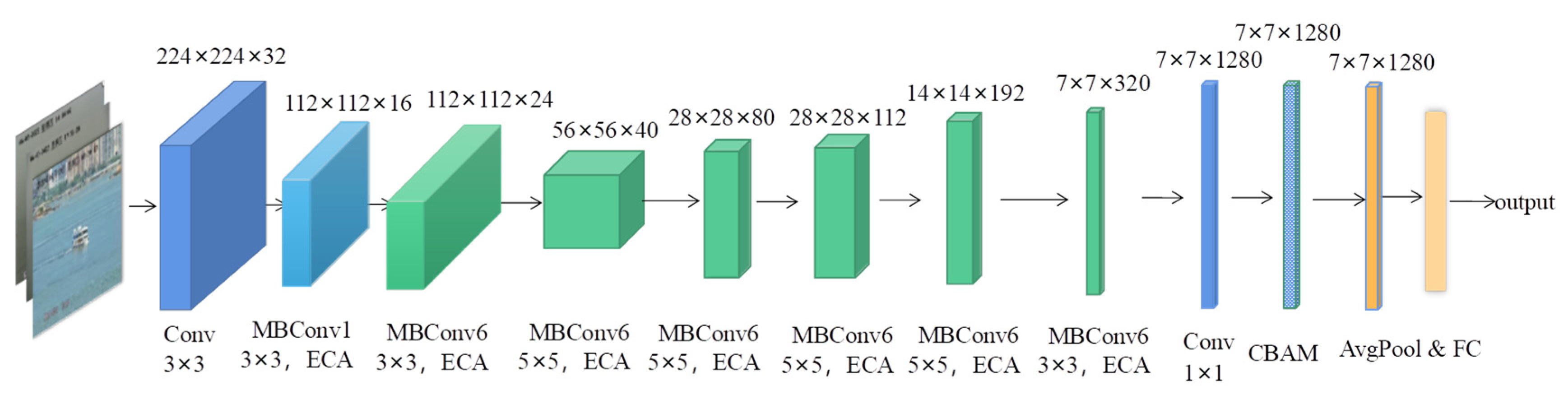
4.1. Overall Model Structure

To reduce the number of model input parameters and facilitate the needed environmental classifications, we constructed our method using a discriminative deep learning architecture that output the fog visibility level. To keep the model small, efficient, and fast, we selected EfficientNet [31] as the classification algorithm. Since the classification ability of the model depended on the extraction of image features in a difficult foggy image, we used the efficient channel attention module (ECA) [32]. We replaced the original squeeze excitation (SE) module and added the convolution block attention module (CBAM) after the last convolution of the EfficientNet network [33]. We optimized the EfficientNet network structure to extract deep features efficiently and adopted global average pooling (AvgPool) and a full connection (FC) method for fog classification with a focus loss function (FocalLoss) during model training [34] to solve the problem of balanced sample numbers. Our classification-perception model is shown in Figure 2.

4.2. The EfficientNet Network

Given the practical computational limitations (measured in FLOPS) of typical computers, EfficientNet analyzes the influence of the network size to find appropriate configuration parameters. The core of the EfficientNet network is a hybrid model scaling (compound model scaling) algorithm that comprehensively optimizes the network depth, width, and resolution, reducing the number of parameters and improving the calculation speed while achieving optimal accuracy [35].
EfficientNet defines the network architecture as a composite model scaling optimization problem and targets the optimal width, depth, and resolution simultaneously. The network parameters and computational requirements must meet certain conditions, as shown in the following equation:
A c c u r a c y N d , w , r d , w , r m a x   s . t . N d , w , r = i = 1 s F ^ i d · L ^ i X r · H ^ i , r · W ^ i , w · C ^ i M e m o r y N t a r g e t _ m e m o r y F L O P S N t a r g e t _ f l o p s .
In Equation (1), N d , w , r represents the classification network; m a x A c c u r a c y is the maximum accuracy of the model; i represents a stage (convolution order); d represents the depth scaling coefficient to scale up L ^ i (the number of convolution layers for the first stage); w represents the width scaling coefficient; C ^ i is the number of channels of the output feature matrix; r represents the resolution scaling coefficient used to affect H ^ i (high preset resolution) and W ^ i (wide preset resolution); F ^ i is the network structure; F ^ i L ^ i represents the repeated L ^ i times in s t a g e i ; X represents the input feature matrix of s t a g e i with dimensions H ˙ i , W ^ i , C ^ i ; i = 1 s represents the continuous multiplication operation; M e m o r y ( N ) represents the number of network parameters; F L O P S ( N ) represents the number of network floating-point computations per second; and t a r g e t _ m e m o r y and t a r g e t _ f l o p s represent the number of target network parameters and the target floating-point operations, respectively.
Further, the unified parameter scaling of the width, depth, and resolution was introduced through the hybrid model scaling algorithm ϕ . The specific relationship is shown in the following equations:
d e p t h : d = α ϕ w i d t h : w = β ϕ r e s o l u t i o n : r = γ ϕ s . t . α · β 2 · γ 2 2 α 1 , β 1 , γ 1 .
In Equation (2), α , β , a n d   γ are constants that indicate how to allocate parameters for depth, width, and resolution resources, respectively; and φ is a mixing factor.
The baseline model was obtained using neural architecture search (NAS) and scaling operations on the depth, width, and input image resolution of EfficientB0 to produce a series of network models (EfficientNets). Table 2 shows the EfficientNet-B0 baseline network structure.
In the EfficientNet-B0 network structure, the first stage consisted of a 3 × 3 convolution layer, batch normalization (BN), and a Swish activation function. Stages 2 through 8 were repeatedly stacked MBConv structures, with the “Layers” column showing the number of MBConv structure repeats. Stage 9 consisted of a 1 × 1 convolution layer, BN, Swish activation function, average pooling layer, and a fully connected layer. Each MBConv in Table 2 is followed by either the number 1 or 6, where the numbers 1 and 6 are the multiple factors; that is, the convolution layer expanded the channels of the input feature matrix to 1 or 6 factors. Furthermore, k3 × 3 or k5 × 5 represents the size of the convolutional kernel that was employed by DWConv in MBConv. The “Channels” column represents the number of channels of the output feature matrix after passing through this stage.
The MBConv structure was mainly composed of a single 1 × 1 ordinary convolution, a k × k DWConv, an SE module, a 1 × 1 ordinary convolution, and a Dropout layer, where the specific values of k were mainly in both the 3 × 3 and 5 × 5 cases[25]. The specific MBConv structure is shown in Figure 3.

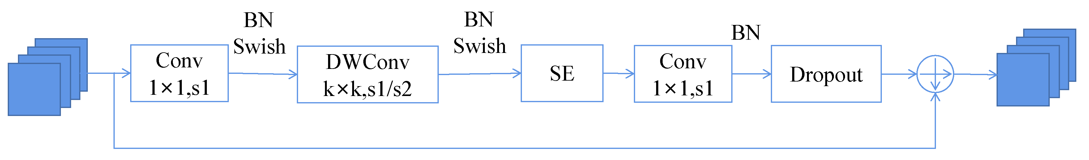
4.3. Optimization of Ship Navigation Fog Environment Classification Model

4.3.1. Improvement of the Attention Mechanism

The basic EfficientNet network uses the SE attention mechanism module to improve the performance of the deep convolutional network. However, the complexity of the SE attention mechanism module is high, the performance improvement of the deep convolutional network is limited, and the extraction results of features relating to fog visibility are not obvious.
Therefore, we selected an efficient channel attention (ECA) module to balance the performance and complexity of the model calculation, reduce the model complexity, and improve the performance of the deep convolutional network. The ECA structural model is shown in Figure 4.
The ECA structure obtains each channel weight w and multiplies the weights with the corresponding elements of the original input feature graph to obtain the final output feature graph [36]. The formula for calculating w is:
ω = σ ( C L D k ( y ) ) .
In Equation (3), y is the global average pooling function, σ is the Sigmoid function, CLD represents the 1 D convolution, and k is the convolution kernel size. The convolution kernel calculation formula is shown in the following equation:
k = log 2 ( C ) γ + b γ o d d .
In Equation (4), C represents the number of channel dimensions; the γ and b coefficients were taken to be 1 and 2; respectively, and k = t o d d represents the odd number nearest to t.
The basic EfficientNet network only considers the coding of the information between the channels and does not consider the spatial location information of the fog and the surrounding environment, which affects the visibility level classification results of the fog environment.
Therefore, we added the CBAM attention module to the basic EfficientNet network to integrate a channel and a spatial attention module for better classification results. The CBAM structural model is shown in Figure 5.
The CBAM formula is as follows:
F = M s F F F = M c F F M c F = σ ( M L P A v g P o o l F + M L P M a x P o o l F ) = σ W 1 W 0 F a v g C + W 1 W 0 F m a x C M s F = σ ( f 7 × 7 ( [ A v g P o o l F + M a x P o o l F ] ) ) = σ f 7 × 7 F a v g C ; F m a x C .
In Equation (5), F represents the input features, F represents the spatial module input features, F represents the final output features, M s represents channel attention, M c represents spatial attention, A v g P o o l represents global average pooling, M a x P o o l represents global maximum pooling, M L P represents the multilayer perceptron, σ represents the Sigmoid activation function, W 1 and W 0 represent the weight of the M L P neurons, and f 7 × 7 represents the utilization size of the 7 × 7 convolution kernel.

4.3.2. Improvement of the Loss Function

In our fog dataset, the dataset samples had such an uneven distribution problem. Therefore, the focal loss function was introduced to reduce the internal weighting, solve the class imbalance problem, reduce the ease of the sample weights of the network in the training process, and focus on the dataset with sparse difficult samples for training. The focal loss formula [37] is shown in Equation (6):
F o c a l p t = 1 p t γ log p t ,
p t = p i f y = 7 1 p o t h e r w i s e
In Equation (6), γ is a constant representing the sample weight, which is used to measure difficult and easy samples; p is the category predicted probability value, which ranges between 0 and 1; and y values ranging from 0 to 7 are used to identify the classes (e.g., y = 1 represents class 1).

5. Comparative Analysis of the Results of the Fog Environment Visibility Experiment

5.1. Classification Experiment of Ship Navigation Fog Environment

To verify the effectiveness of our model, we analyzed our dataset and conducted ablation experiments along with performance measurements of the classification results.

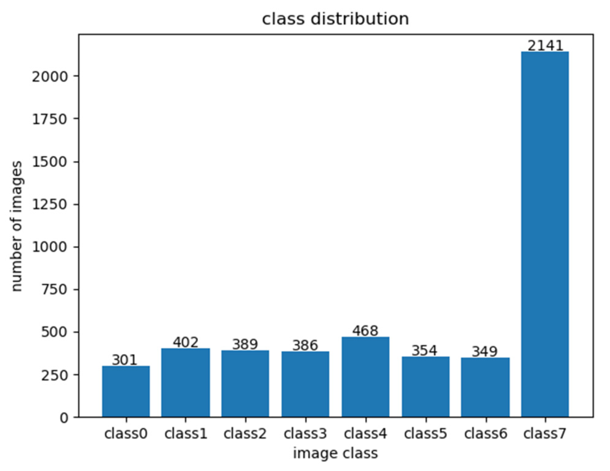
5.1.1. Description of the Fog Environment Visibility Dataset

The dataset contained 4790 images divided into eight categories. Figure 6 shows the statistical results of the dataset. Its main features included an uneven distribution of dataset samples, with the first label having the fewest samples (301 pictures) and the eighth sample having the most (2141 pictures). The resolution of the dataset images was constant at 704 × 576 pixels.

5.1.2. Ablation Experiment of Ship Navigation Fog Environment Classification Model

According to the classification requirements of our environment, accuracy (Accuracy) was the main evaluation index combined with the cumulative operator (MACS), the number of model parameters, and the model size. The accuracy calculation formula is as follows:
A c c u r a c y = T P + T N T P + T N + F N + T N × 100 % .
In Equation (8), TP, FP, FN, and TN represent the number of positive samples correctly identified (true positives), the number of misreported negative samples (false positives), the number of negative samples incorrectly identified (false negatives), and the number of negative samples correctly identified (true negatives), respectively.
Ablation experiments refer to the use of laboratory techniques to detect the impact of certain model components (such as layers, features, parameters, etc.) on model performance by removing or blocking them. To verify the effectiveness of our model, we performed the following four ablation experiments:
(1)
Basic EfficientNet using the basic EfficientNet network for training;
(2)
EfficientNet + ECA using the ECA attention module based on Equation (1) to replace the SE module in the MBConv structure;
(3)
EfficientNet + ECA + BAM with the CBAM attention module added after the last convolutional layer based on Equation (2); and
(4)
Based on (3), the focus loss function was used to form the final improved EfficientNet model.
The results of the ablation experiments are shown in Table 3.
Based on the experiments summarized in the table, we drew the following conclusions.
  • When comparing Models (1) and (2), replacing the SE module with the ECA attention module improved the accuracy by 0.21% and reduced the MACS, the number of parameters, and the model size, showing that the ECA module was lighter and offered a stronger attention learning ability than the SE module.
  • When comparing Models (3) and (2), the results showed that adding the CBAM attention module increased the accuracy of MACS with only a slight increase of 0.07% in the number of parameters and the model size, indicating that adding CBAM extracted better network features with greater accuracy.
  • When comparing Models (4) and (3), the results showed that the focus loss function reaction model accelerated the network learning. Under the same input conditions, the accuracy of Model (4) was improved by 0.06%.
To sum up, the EfficientNet model was effective in improving the model. The accuracy of the model reached 95.05% in the validation set, with 0.401 G MACS, 4.20 M model parameters, and a model size of 16.31 MB. Relative to the underlying EfficientNet model, the accuracy of the improved perception model improved by 0.42%, and the lighter-weight model preserved a high accuracy.

5.1.3. Classification Performance Analysis of Ship Navigation Fog Environment

The visibility grade classification results are shown in Table 1. After classifying the validation set data, the confusion matrix was drawn statistically for all images to show the classification results. The confusion matrix diagram is shown in Figure 6.
Figure 7 shows that the overall accuracy of ship navigation fog environment classification reached 95.05%, with good performance in all grades. The data were mainly concentrated on the diagonal and adjacent points, with a small number of misclassified data categories. According to these results, we considered our model’s performance stable and reliable.

5.2. Visibility Enhancement Experiment of Ship Fog Environment

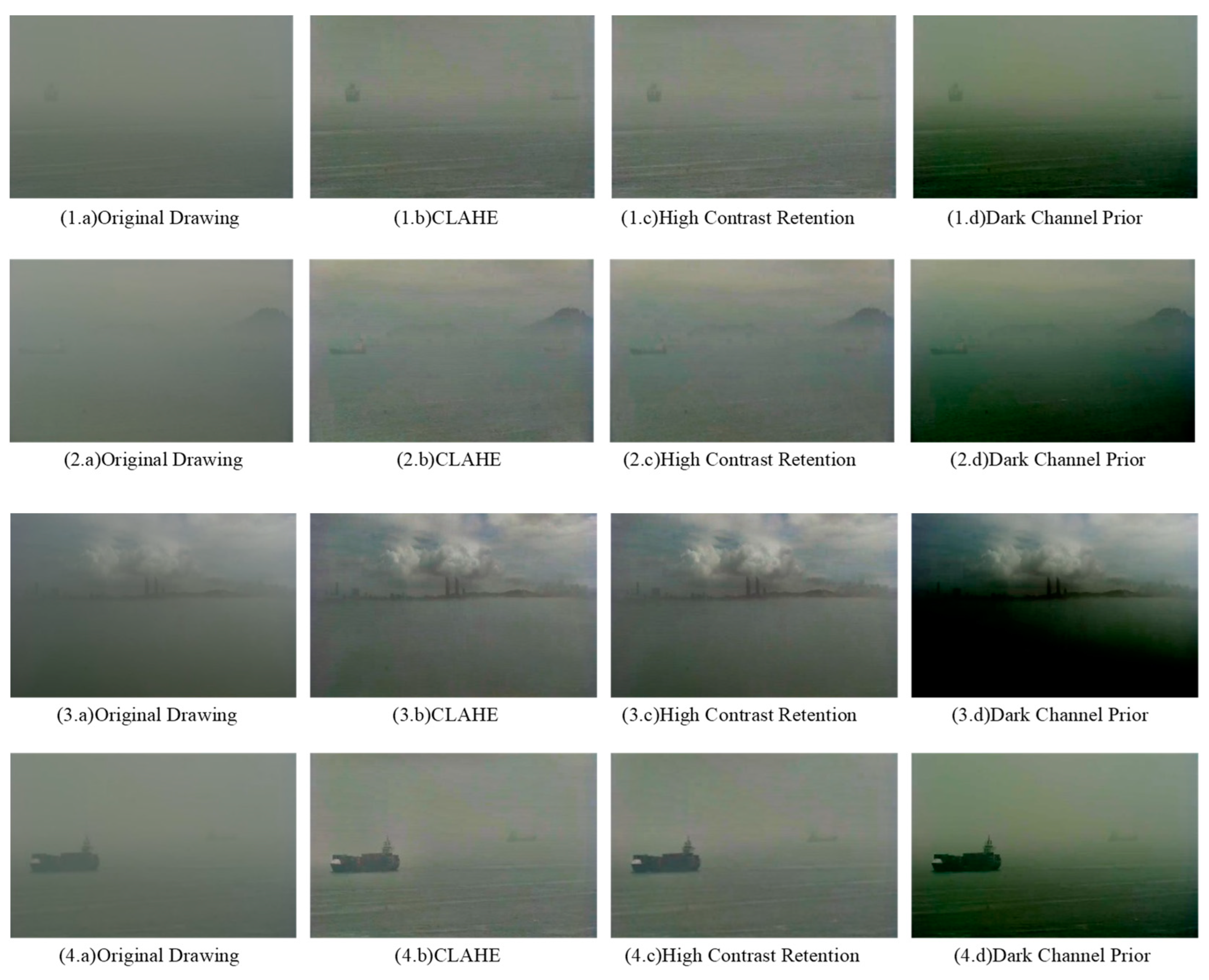
5.2.1. Comparison of Visibility Enhancement Experiment in Fog Environment

To verify the effectiveness of our enhancement algorithm, we used high-contrast retention, CLAHE, and a dark channel algorithm for a visibility enhancement experiment. The specific process was as follows:
  • Samples in dataset classes 0–6 were processed with each augmentation algorithm;
  • The classification model presented in this paper was used to classify the images processed in the previous step;
  • The image-processing classification results were compared with the original image level to determine whether the visibility level was improved and whether the improvement was effectively enhanced;
  • The ratio of the effective enhancement number of each level and the number of samples in the corresponding level in different datasets were calculated to obtain the effective enhancement rate.
This article determined the experimental results of the enhancement model for different visibility levels by comparing the application of different image resolutions and different models. According to the experimental results in Table 4, all three algorithms enhanced visibility. The high-contrast retention algorithm had the best results in class 6. The CLAHE algorithm was more prominent in classes 0 and 3, and the dark channel prior algorithm was outstanding in classes 1, 2, 4, and 5.

5.2.2. Results of Visibility Enhancement in Fog Environment

The EfficientNet neural network alone does not directly improve visibility perception. In this manuscript, we utilized the EfficientNet neural network to classify visibility levels and applied existing algorithms such as high-contrast retention, CLAHE, and dark channel enhancement to enhance visibility for different visibility levels. Compared with the original image, a subjective review of the processed images showed that all three algorithms enhanced the visibility and environmental perception, as shown in Figure 8.

6. Conclusions

Given the requirements of safely navigating ships in foggy conditions, we constructed a ship navigation fog environment classification model using deep learning and determined the optimal enhancement algorithm for each type of fog according to the classification results to produce better perception results for navigation. This laid a foundation for intelligent unmanned and remotely operated ships. Our detailed conclusions were as follows.
(1)
We constructed a fog environment classification image dataset using visibility grade classification rules and perceived visibility.
(2)
Using this dataset, we designed a perceived visibility model structure using a discriminant deep learning architecture and the EfficientNet neural network while adding the CBAM, focal loss, and other improvements. Our experiments showed that our model’s accuracy exceeded 95%, which meets the needs of intelligent ship navigation in foggy conditions.
(3)
Using our model and the dataset, we were able to determine the best image-enhancement algorithm based on the type of fog detected. The dark channel prior algorithm worked best with fog classes 1, 2, 4, and 5. The CLAHE algorithm worked best with fog classes 0 and 3. The high-contrast retention algorithm worked best with fog class 6.

Author Contributions

C.W., B.F., Y.L. and S.Z. proposed the idea and derived the algorithm; J.X., L.M. and J.Z. were responsible for the code testing and algorithm results; B.F., Y.L. and R.W. wrote the algorithm and conducted the experiments; J.C., Z.L. and S.S. performed the dataset collection and identification; C.W., B.F., Y.L. and S.Z. performed the theoretical calculations; C.W., B.F., Y.L. and S.Z. wrote the manuscript. All authors analyzed the data, discussed the results, and commented on the manuscript. All authors have read and agreed to the published version of the manuscript.

Funding

This research was funded by the Xiamen Ocean and Fishery Development Special Fund Project grant number No. 21CZBO14HJ08 and the Ship Scientific Research Project—Key technology and demonstration of type 2030 green and intelligent ship in Fujian region grant number No. CBG4N21-4-4.

Institutional Review Board Statement

Not applicable.

Informed Consent Statement

Not applicable.

Data Availability Statement

Not applicable.

Acknowledgments

We thank LetPub (www.letpub.com, accessed on 19 May 2023) for its linguistic assistance during the preparation of this manuscript.

Conflicts of Interest

The authors declare no conflict of interest.

References

  1. Ye, Y.; Chen, Y.; Zhang, P.; Cheng, P.; Zhong, H.; Hou, H. Traffic Accident Analysis of Inland Waterway Vessels Based on Data-driven Bayesian Network. Saf. Environ. Eng. 2022, 29, 47–57. [Google Scholar]
  2. Zhen, G. Discussion on the safe navigation methods of ships in waters with poor visibility. China Water Transp. 2022, 4, 18–20. [Google Scholar]
  3. Khan, S.; Goucher-Lambert, K.; Kostas, K.; Kaklis, P. ShipHullGAN: A generic parametric modeller for ship hull design using deep convolutional generative model. Comput. Methods Appl. Mech. Eng. 2023, 411, 116051. [Google Scholar] [CrossRef]
  4. Wright, R.G. Intelligent autonomous ship navigation using multi-sensor modalities. Trans. Nav. Int. J. Mar. Navig. Saf. Sea Transp. 2019, 13, 3. [Google Scholar] [CrossRef]
  5. Varelas, T.; Archontaki, S.; Dimotikalis, J.; Turan, O.; Lazakis, I.; Varelas, O. Optimizing ship routing to maximize fleet revenue at Danaos. Interfaces 2013, 43, 37–47. [Google Scholar] [CrossRef]
  6. Wang, Q.; Wu, B.; Zhu, P.; Li, P.; Zuo, W.; Hu, Q. ECA-Net: Efficient channel attention for deep convolutional neural networks. In Proceedings of the IEEE/CVF Conference on Computer Vision and Pattern Recognition, Seattle, WA, USA, 13–19 June 2020. [Google Scholar]
  7. Zhang, D.; Zhao, Y.; Cui, Y.; Wan, C. A Visualization Analysis and Development Trend of Intelligent Ship Studies. J. Transp. Inf. Saf. 2021, 39, 7–16+34. [Google Scholar]
  8. Pedersen, M.; Bruslund Haurum, J.; Gade, R.; Moeslund, T.B. Detection of marine animals in a new underwater dataset with varying visibility. In Proceedings of the IEEE/CVF Conference on Computer Vision and Pattern Recognition Workshops, Long Beach, CA, USA, 15–20 June 2019. [Google Scholar]
  9. Kim, D.; Park, M.S.; Park, Y.J.; Kim, W. Geostationary Ocean Color Imager (GOCI) marine fog detection in combination with Himawari-8 based on the decision tree. Remote Sens. 2020, 12, 149. [Google Scholar] [CrossRef] [Green Version]
  10. Cornejo-Bueno, S.; Casillas-Pérez, D.; Cornejo-Bueno, L.; Chidean, M.I.; Caamaño, A.J.; Cerro-Prada, E.; Casanova-Mateo, C.; Salcedo-Sanz, S. Statistical analysis and machine learning prediction of fog-caused low-visibility events at A-8 motor-road in Spain. Atmosphere 2021, 12, 679. [Google Scholar] [CrossRef]
  11. Palvanov, A.; Young, I.C. Visnet: Deep convolutional neural networks for forecasting atmospheric visibility. Sensors 2019, 19, 1343. [Google Scholar] [CrossRef] [Green Version]
  12. Huang, L.; Zhang, Z.; Xiao, P.; Sun, J.; Zhou, X. Classification and application of highway visibility based on deep learning. Trans. Atmos. Sci. 2022, 45, 203–211. [Google Scholar]
  13. Deniz, E.; Anıl, G.; Hazım Kemal, E. Cycle-Dehaze: Enhanced CycleGAN for Single Image Dehazing. arXiv 2018, arXiv:1805.05308. [Google Scholar]
  14. Yuanjie, S.; Lerenhan, L.; Wenqi, R.; Changxin, G.; Nong, S. Domain Adaptation for Image Dehazing. In Proceedings of the IEEE/CVF Conference on Computer Vision and Pattern Recognition (CVPR), Seattle, WA, USA, 13–19 June 2020; pp. 2808–2817. [Google Scholar]
  15. Qin, X.; Wang, Z.; Bai, Y.; Xie, X.; Jia, H. FFA-Net: Feature Fusion Attention Network for Single Image Dehazing. In Proceedings of the AAAI Conference on Artificial Intelligence, New York, NY, USA, 7–12 February 2020; Volume 34, pp. 11908–11915. [Google Scholar]
  16. Park, J.; Han, D.K.; Ko, H. Fusion of Heterogeneous Adversarial Networks for Single Image Dehazing. IEEE Trans. Image Process. 2020, 29, 4721–4732. [Google Scholar] [CrossRef] [PubMed]
  17. Wu, H.; Qu, Y.; Lin, S.; Zhou, J.; Qiao, R.; Zhang, Z.; Xie, Y.; Ma, L. Contrastive Learning for Compact Single Image Dehazing. In Proceedings of the IEEE/CVF Conference on Computer Vision and Pattern Recognition (CVPR), Nashville, TN, USA, 19–25 June 2021; pp. 10551–10560. [Google Scholar]
  18. Ullah, H.; Muhammad, K.; Irfan, M.; Anwar, S.; Sajjad, M.; Imran, A.S.; de Albuquerque, V.H.C. Light-DehazeNet: A Novel Lightweight CNN Architecture for Single Image Dehazing. IEEE Trans. Image Process. 2021, 30, 8968–8982. [Google Scholar] [CrossRef]
  19. Koschmieder, H. Theorie der horizontalen sichtweite. Beitr. Phys. Freien Atmos. 1924, 33–53, 171–181. [Google Scholar]
  20. Middleton, W. Vision through the Atmosphere; University of Toronto Press: Toronto, ON, Canada, 1952. [Google Scholar]
  21. Redman, B.J.; van der Laan, J.D.; Wright, J.B.; Segal, J.W.; Westlake, K.R.; Sanchez, A.L. Active and Passive Long-Wave Infrared Resolution Degradation in Realistic Fog Conditions; No. SAND2019-5291C; Sandia National Lab (SNL-NM): Albuquerque, NM, USA, 2019. [Google Scholar]
  22. Lu, T.; Yang, J.; Deng, M. A Visibility Estimation Method Based on Digital Total-sky Images. J. Appl. Meteorol. Sci. 2018, 29, 63–71. [Google Scholar]
  23. Kaiming, H.; Jian, S.; Xiaoou, T. Single Image Haze Removal Using Dark ChannelPrior. In Proceedings of the IEEE Conference on Computer Vision and Pattern Recognition (CVPR), Miami Beach, FL, USA, 20–26 June 2009; pp. 1956–1963. [Google Scholar]
  24. Ortega, L.; Otero, L.D.; Otero, C. Application of machine learning algorithms for visibility classification. In Proceedings of the 2019 IEEE International Systems Conference (SysCon), Orlando, FL, USA, 8–11 April 2019; IEEE: Piscataway, NJ, USA, 2019. [Google Scholar]
  25. Huang, L. Wenyuan Bridge. Navigation Meteorology and Oceanography. Hubei; Wuhan University of Technology Press: Wuhan, China, 2014. [Google Scholar]
  26. Li, Z.; Che, W.; Qian, M.; Xu, X. An Improved Image Defogging Algorithm Based on Histogram Equalization. Henan Sci. 2021, 39, 1–6. [Google Scholar]
  27. Zhu, Y.; Lin, J.; Qu, F.; Zheng, Y. Improved Adaptive Retinex Image Enhancement Algorithm. In Proceedings of the ICETIS 2022, 7th International Conference on Electronic Technology and Information Science, Harbin, China, 21–23 January 2022; pp. 1–4. [Google Scholar]
  28. Wen, H.; Li, J. An adaptive threshold image enhancement algorithm based on histogram equalization. China Integr. Circuit 2022, 31, 38–42+71. [Google Scholar]
  29. Fang, D.; Fu, Q.; Wu, A. Foggy image enhancement based on adaptive dynamic range CLAHE [J/OL]. Laser Optoelectron. Prog. 2022, 9, 1–14. [Google Scholar]
  30. Yin, J.; He, J.; Luo, R.; Yu, W. A Defogging Algorithm Combining Sky Region Segmentation and Dark Channel Prior. Comput. Technol. Dev. 2022, 32, 216–220. [Google Scholar]
  31. Tan, M.; Le, Q.V. EfficientNet: Rethinking model scaling for convolutional neural networks. In Proceedings of the International Conference on Machine Learning, PMLR, Long Beach, CA, USA, 9–15 June 2019. [Google Scholar]
  32. Nayak, D.R.; Padhy, N.; Mallick, P.K.; Zymbler, M.; Kumar, S. Brain tumor classification using dense efficient-net. Axioms 2022, 11, 34. [Google Scholar] [CrossRef]
  33. Woo, S.; Park, J.; Lee, J.Y.; Kweon, I.S. Cbam: Convolutional block attention module. In Proceedings of the European Conference on Computer Vision (ECCV), Munich, Germany, 8–14 September 2018; pp. 3–19. [Google Scholar]
  34. Lin, T.Y.; Goyal, P.; Girshick, R.; He, K.; Dollár, P. Focal loss for dense object detection. In Proceedings of the IEEE International Conference on Computer Vision, Venice, Italy, 22–29 October 2017; pp. 2980–2988. [Google Scholar]
  35. Goswami, V.; Sharma, B.; Patra, S.S.; Chowdhury, S.; Barik, R.K.; Dhaou, I.B. IoT-Fog Computing Sustainable System for Smart Cities: A Queueing-based Approach. In Proceedings of the 2023 1st International Conference on Advanced Innovations in Smart Cities (ICAISC), Jeddah, Saudi Arabia, 23–25 January 2023. [Google Scholar]
  36. Li, X.; Wang, W.; Wu, L.; Chen, S.; Hu, X.; Li, J.; Tang, J.; Yang, J. Generalized focal loss: Learning qualified and distributed bounding boxes for dense object detection. Adv. Neural Inf. Process. Syst. 2020, 33, 21002–21012. [Google Scholar]
  37. Thombre, S.; Zhao, Z.; Ramm-Schmidt, H.; Garcia, J.M.V.; Malkamaki, T.; Nikolskiy, S.; Hammarberg, T.; Nuortie, H.; Bhuiyan, M.Z.H.; Sarkka, S.; et al. Sensors and AI techniques for situational awareness in autonomous ships: A review. IEEE Trans. Intell. Transp. Syst. 2020, 23, 64–83. [Google Scholar] [CrossRef]
Figure 1. Samples of different types of fog from the image dataset.
Jmse 11 01298 g001
Figure 2. Structural diagram of the ship navigation fog environment perception classification model.
Jmse 11 01298 g002
Figure 3. MBConv structural diagram.
Jmse 11 01298 g003
Figure 4. The ECA structural model.
Jmse 11 01298 g004
Figure 5. CBAM and the structural model.
Jmse 11 01298 g005
Figure 6. Dataset label distribution.
Jmse 11 01298 g006
Figure 7. Model confusion matrix plot.
Jmse 11 01298 g007
Figure 8. Visibility enhancement results.
Jmse 11 01298 g008aJmse 11 01298 g008b
Table 1. Visibility classification rules in foggy environments.
Visibility ScalePerceived DistanceWeather Conditions
NMKm
0 ≤0.05≤0.1
1 0.05–0.100.1–0.2Heavy fog, fog
2 0.10.–0.250.20–0.5Dense fog
3 0.250–0.500.50–1.0Fog, light fog
4 0.500–1.000.01–2.0Mist
5 0.01–2.00.02–4.0Moderate rain, light fog
6 2–54–10Light rain, light fog
7 ≥5≥10Drizzle, light rain, no fog
Table 2. The EfficientNet-B0 baseline network structure.
Stage (Convolution Order)OperatorResolution# of Channels# of Layers
i F i H i × W i C i L i
1Conv3 × 3224 × 224321
2MBConv1, k3 × 3112 × 112161
3MBConv6, k3 × 3112 × 112242
4MBConv6, k5 × 556 × 56402
5MBConv6, k3 × 328 × 28803
6MBConv6, k5 × 514 × 141123
7MBConv6, k5 × 514 × 141924
8MBConv6, k3 × 37 × 73201
9Conv 1 × 1 & Pool & FC7 × 712801
Table 3. Ablation experiments of ship navigation fog environment classification model.
Computational ModelPrecision/%MACs/GParticipants/MModel Size/MBFPS
Model 1: original EfficientNet94.630.3984.0215.6235.7
Model 2: EfficientNet + ECA94.840.4003.3813.1834.1
Model 3: EfficientNet + ECA + CBAM94.910.4014.2016.3138.5
Model 4: the model in this paper95.050.4014.2016.3142.9
Table 4. Comparison of visibility enhancement experiments.
Enhanced AlgorithmCLASS 0CLASS 1CLASS 2CLASS 3CLASS 4CLASS 5CLASS 6
HIGH-CONTRAST RETENTION71.76%45.9%40.36%26.17%26.6%28.81%29.80%
clahe76.08%19.16%51.16%27.46%10.04%29.67%24.64%
DARK CHANNEL PRIORS51.50%48.26%73.26%22.54%29.49%48.59%23.50%
Disclaimer/Publisher’s Note: The statements, opinions and data contained in all publications are solely those of the individual author(s) and contributor(s) and not of MDPI and/or the editor(s). MDPI and/or the editor(s) disclaim responsibility for any injury to people or property resulting from any ideas, methods, instructions or products referred to in the content.

