Article

Method for Identifying Materials and Sizes of Particles Based on Neural Network

1
Marine Engineering Collage, Dalian Marinetime University, Dalian 116026, China
2
School of Ocean Engineering, Harbin Institute of Technology, Weihai 264209, China
3
Shandong Institute of Shipbuilding Technology, Weihai 264209, China
4
School of Information Science and Engineering, Harbin Institute of Technology, Weihai 264209, China
5
School of Biomedical Engineering, Shanghai Jiao Tong University, Shanghai 200240, China
*
Author to whom correspondence should be addressed.
J. Mar. Sci. Eng. 2023, 11(3), 541; https://doi.org/10.3390/jmse11030541
Submission received: 22 December 2022 / Revised: 15 February 2023 / Accepted: 24 February 2023 / Published: 2 March 2023
(This article belongs to the Special Issue Advances in Sensor Technology in Smart Ships and Offshore Facilities)

Abstract

:
Ships are equipped with power plants and operational assistance devices, both of which need oil for lubrication or energy transfer. Oil carries a large number of metal particles. By identifying the materials and sizes of metal particles in oil, the position and type of wear can be fully understood. However, existing online oil-detection methods make it difficult to identify the materials and the sizes of metal particles simultaneously and continuously. In this paper, we proposed a method for identifying the materials and the sizes of particles based on neural network. Firstly, a tree network model was designed. Then, each sub-network was trained in stages. Finally, the identification performance of several key groups of different frequencies and frequency combinations was tested. The experimental results showed that the method was effective. The accuracies of material and size identification reached 98% and 95% in the pre-training stage, and both had strong robustness.

1. Introduction

In the field of marine engineering, the hydraulic system is widely used, and oil is the key working medium of hydraulic system [1]. As complex systems, ships are equipped with power plants and many operational assistance devices, which all require oil as a lubricant or energy transfer medium. During the operation of machines, metal particles peel off the friction pairs for various reasons and flow with the oil. Statistics show that more than 75% of hydraulic system failures, about 35% of diesel engine operation failures, 38.5% of gear failures and 40% of rolling bearing failures are caused by oil failures [2,3]. Each particle in the oil is an important information carrier. The wear mode can be judged by the quantity distribution of the particles, and the wear position can be judged by the particle material. Particle detection is very important for predicting potential trouble and avoiding catastrophic failures [4].
There are many kinds of analytical methods for oil particles, which can basically be divided into three categories: particle size distribution analytical method, particle material analysis method, and a combination of the two. The particle size distribution analytical method is as follows: the particle size is measured, and particles are counted according to the particle size interval to form a particle size distribution. The particle size distribution is compared with the cleanliness standard to determine the cleanliness level of the oil. The particle material analytical method involves using the particularity of materials to analyze the composition of particles, so as to determine the source of particles and the abnormal wear of components [5,6].
The combination of the particle size distribution analytical method and particle material analytical method allows one to diagnose the wear condition at a given location by classifying the particle material along with particle counting and size measurement. In offline detection, there are many analytical methods, such as ferrography and spectroscopy [7], but the information about materials and sizes cannot be obtained simultaneously. Online detection can be used to monitor the oil condition in real-time, and the manual requirements are low, in line with the development trend of the industry. Particle detection methods with classification ability include the inductance detection method [8], the capacitance detection method [9], the ultrasonic detection method [10], the image recognition method [11], and the optical method [12]. The principles, advantages, and disadvantages of these methods are shown in Table 1.
At present, the analytical method combining particle size distribution and particle material in the above table can only be used to roughly identify particles, especially material. Oil analytical technology combining multiple methods can obtain particle size distributions and element information. However, because the two kinds of information are obtained by different instruments at different times, it is difficult to integrate the two kinds of information, and it is not possible to make a one-to-one correspondence between size and material, resulting in the failure to trace the source and wear form of particles. In view of the problem that various methods cannot identify particle size information and material information simultaneously, a method for identifying the materials and the sizes of particles based on neural network is proposed in this study.

2. Particle Identification and Particle Signal Characteristics

2.1. Particle Signal and Feature Simulation

The basic principle of particle detection is the same for both through-stream and side-stream inductance coils. An alternating magnetic field is used to induce a tiny vortex electric field inside the through-stream particles, and this field moves with the liquid flow in the detection space to excite the particle magnetic field. The particle magnetic field produces a weak change in impedance or voltage of the sensor coil. In the early stage of particle detection, the number of particles is detected and recorded by the number of changes in impedance or voltage [13]. In order to quantify the detection signal and the relationship between particle material and particle size, as shown in Figure 1, our research group [14] previously established a magnetization characteristics model of metal particles in a time-harmonic magnetic field. According to this model, the form of particle signal under different detection methods was provided. When the particles passed through the detection area of the coil along a certain track, the impedance signal was generated as follows:
Δ R r = μ 0 ω v p imag χ h r 2 ,
Δ L r = μ 0 v p real χ h r 2 ,
χ = 3 2 2 μ r + 1 a 2 k 2 sin a k + a k 2 μ r + 1 cos a k μ r 1 + a 2 k 2 sin a k a k μ r 1 cos a k ,
where Δ R r is the resistance signal, representing changes in the resistance of the coil impedance caused by a particle at r ; Δ L r is the inductance signal, representing changes in the inductance of the coil impedance caused by a particle at r ; ω represents the angular frequency of the excitation current; μ 0 represents the vacuum permeability constant, which is usually 4 π × 10 7 H / m ; v p represents equivalent spherical volume of particle; a is radius of particle; χ is a complex variable representing the magnetic susceptibility of metal particles in a time-harmonic magnetic field; k is a constant, with a value of k = j ω μ 0 μ r σ ; μ r and σ are relative permeability and conductivity of particle, respectively; h r is a space vector representing the magnetic field intensity at r when one unit of DC is applied to the coil; j is an imaginary number unit.
As shown in Figure 1, when a particle passes through the detection area of the coil along a certain track, the impedance signal is generated. The impedance signal is comprised of the resistance signal Δ R r and the inductance signal Δ L r . r represents the position of the particle. The resistance signal and the inductance signal are pulse signals. One of the signal characteristics is amplitude; that is, the corresponding signal on the track is the largest. These maximum values are called Δ R max and Δ L max , respectively. Other characteristics, such as the modulus of complex impedance change Δ Z and phase angle θ , are described in Equations (4) and (5). The conductivity and permeability of different material particles are shown in Table 2.
Δ Z = Δ R max 2 + ω 2 Δ L max 2
θ = arctan ω Δ L m a x Δ R m a x

2.2. Selection of Experimental Particles

Commonly used mechanical engineering materials, such as copper, iron, aluminum, and their alloys, need to be identifiable. In this study, eight granular materials were identified, namely, iron (Fe), copper (Cu), aluminum (Al), nodular iron, cobalt (Co), Ni-Co alloy, brass, and permalloy.
According to the SRM P2806B standard of the National Institute of Standards and Technology (NIST) [15], particle size can be divided into five categories: 6~14 μ m , 14~21 μ m , 21~38 μ m , 38~70 μ m , and >70 μ m . This standard has reasonable division, meeting the service requirements of measurement value transmission in the field of particle counting, and is beneficial to measurement management and unity. Consequently, this standard has been widely used in particle detection and possesses high recognition and credibility.

2.3. Characteristics of Particle Signals in a Complex Plane

Based on Equations (1) and (2) and Table 2, the particle sizes range from 6 to 150 μ m . By changing the particle volume, the curves of eight kinds of particles at frequencies of 41.3 kHz, 0.1 MHz, 1 MHz, and 2 MHz were drawn, as shown in Figure 2.
In this study, we used Δ R and Δ L to identify particles. When two kinds of particles’ Δ R and Δ L values differ significantly, they can be easily classified. As can be seen from Figure 2, there are obvious characteristic differences between ferromagnetic particles and non-ferromagnetic particles. Ferromagnetic particles can produce larger Δ L values than non-ferromagnetic particles and can be easily classified at low frequencies. The permeability of non-ferromagnetic particles is almost the same, but only the conductivity can create a significant difference in Δ R . However, at low frequencies, little discrepancy in Δ L and θ can be seen between different particles. Therefore, only by increasing the frequency can non-ferromagnetic particles have certain identification potential.
Among them, Cu, Fe, Al, and 304 stainless steel sare common metal materials used for mechanical components and have good separability in the characteristic diagrams of these frequencies.
Current particle identification algorithms are only limited to manually identifying ferromagnetic particles and non-ferromagnetic particles, or to distinguishing ferromagnetic particles at a single frequency, lacking accurate material and size identification supported by more data. Based on the above analysis, we propose the hypothesis that the material and particle size of various ferromagnetic and non-ferromagnetic particles can be identified under muti-frequency measurement using deep learning.
Therefore, based on the theories outlined in Section 1 and Section 2, we designed and trained a neural network model, and tested its identification performance during training.

3. Neural Network Particle Identification Model with Pre-Training

This section provides details of the design and training of a particle identification neural network model that includes material and size identification. Section 3.1 describes the structure of the network. Section 3.2 introduces the specific implementation steps of the training.

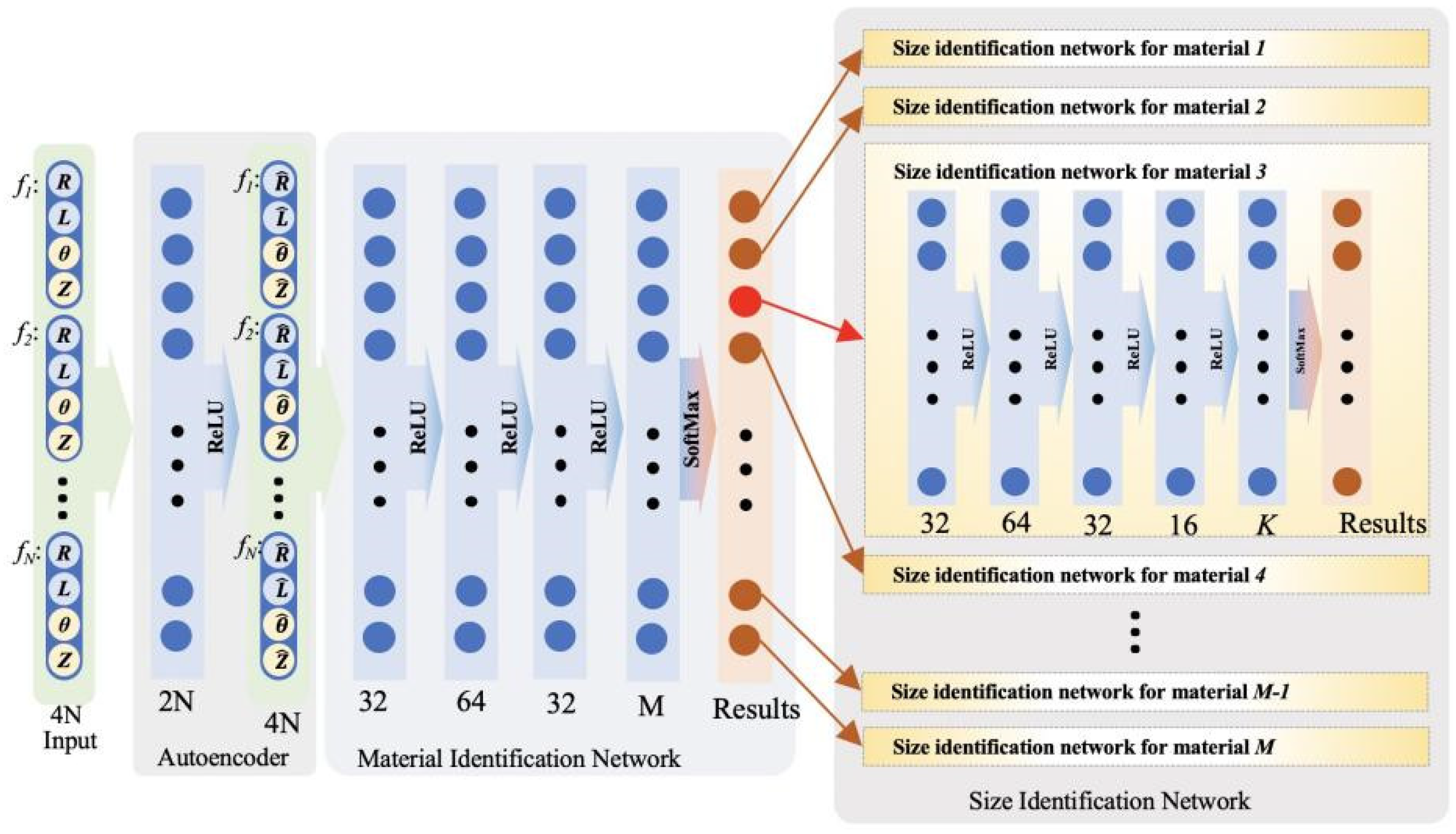
3.1. Neural Network Structure

Figure 3 shows the structure of the neural network for particle identification. Four features were generated for each particle. N represents the number of particles. M represents the number of kinds of materials, which was eight in this study. K represents the number of kinds of sizes, which was 5 in this study. The number at the bottom of the layer represents the amount of output data. The network is composed of an autoencoder (AE), a particle material identification network, and a particle size identification network. The training and identification proccesures are shown in Figure 4. During particle identification, the particle signal obtained by the sensor was processed and input into the encoder to correct the signal drift caused by the experimental environment. Then, the modified data were fed into the material identification network to obtain the identification results of eight kinds of materials. The most general case was used in this paper. Finally, the modified data were fed into the size identification network, and five kinds of size identification results were obtained. The results of each material corresponded to a size identification network. Thus, the whole structure was a tree network structure, with strong readability.

3.1.1. Autoencoder

The actual experimental environment was not completely ideal; for example, the sensor parameters lead to unknown bias gain in the amplitude and phase of the signal. The pre-training needs to train the network with theoretical values, so we needed to correct the drift data. An autoencoder was prepared after the input. The middle layer of the autoencoder structure compressed the dimensions to 1/2 of the input. So this compression did not affect valid information, we needed to nonlinearly expand the input information so that half of the input data came from the amplification. Yehui Li et al. found that, under impedance detection, the particle material and the phase angle are related to the particle size and the modulus of complex number [16]. Therefore, the input of the autoencoder consisted of two parts, the modulus of complex number Z and the phase angle θ as embedding, in addition to the directly measured particle information Δ R max and Δ L max .

3.1.2. Material Identification and Size Identification Network

The material identification network consisted of three dense layers with ReLU and one dense layer with softmax. The size identification network basically adopted a similar structure. The addition of batch normalization between layers results in a wider range of size identification with better robustness [17].
The particle size was more difficult to identify than the material, so the dataset first passed through the material identification network. A network was trained for every particle, rather than all in one network. Although multiple groups of networks were added, the individual scale and training parameters were reduced, and the fitting difficulty of each network was greatly decreased. Thus, the cumulative complexity was much smaller than that of a single network.

3.2. Neural Network Model Pre-Training and Autoencoder Training

The particle identification neural network model needs to undergo two stages of training. In the first stage, the training dataset comprises a large number of data randomly generated by the computer according to formulas. Firstly, the autoencoder is trained to make its output equal to the input, and then the material identification and particle size identification networks are trained. In the second stage, the material identification and particle size identification networks are fixed, and the training dataset comprises the particle data with known information in the experiment. The autoencoder is trained to learn the error of the experimental environment.

3.2.1. First-Stage Training

Pre-training is widely used in natural language processing and computer vision. It is designed to train the network with a structure similar to the sample, so that the network structure has a certain identification potential [18,19]. For example, the Visual Geometry Group (VGG) image recognition network proposed by the University of Oxford is divided into a convolutional feature extraction layer and a subsequent full-connection classification layer [20]. A large amount of pre-training can ensure that the convolutional network part has strong feature extraction ability, and the subsequent training of real dataset focuses on the fully connected part of the classification. In particle identification, it is difficult to obtain signals with particles of known material and size, so pre-training is also needed to reduce its cost. In the first stage, before the pre-training, the autoencoder needs to be trained approximately to make its output equal to its input. Thus, pre-training is equivalent to producing particles in an ideal sensor and training them.
Particles with a scale ranging from 6 to 150 μ m were randomly generated, and the corresponding characteristic information input network was calculated according to Equations (1)–(5). The loss function of pre-training was the cross-entropy function. During pre-training, an Adam optimization algorithm [21,22,23] was adopted to carry out 30,000 iterations of the network, and the batch processing capacity of each iteration was 1000. The initial learning rate was set to 0.001, and the learning rate decayed to half of the previous rate every 3000 iterations. Gradually increasing the noise generated by the sample increased the uncertainty by 0.1% every 6000 iterations.

3.2.2. Second-Stage Training

In the second stage, the identification layer was iterated 50 times using the high-cost real measurement data, so that the identification layer learned the errors created by the environment. The cascading large-scale network parameters were fixed beforehand. Data can lack scale information to reduce the difficulty of acquisition. The learning rate was set to 0.01 with no attenuation. Therefore, the training times could be reduced to ensure that the network convergence occurred as soon as possible.

4. Evaluation and Discussion of Pre-Training Identification Performance

Particle datasets were generated by applying Equations (1)–(3) with particle material random selection from Table 2 and with particle size random from 6 μ m to 150 μ m . To investigate the influences of frequency, datasets of different frequency combinations were used for training and test. The sizes of training datasets and test datasets were 40,000 and 10000, respectively. Dataset 1, Dataset 3, Dataset 5, and Dataset 7 in Table 3 were utilized to train the network. Dataset 2, Dataset 4, Dataset 6, and Dataset 8 were utilized to test network and to calculate performance results.

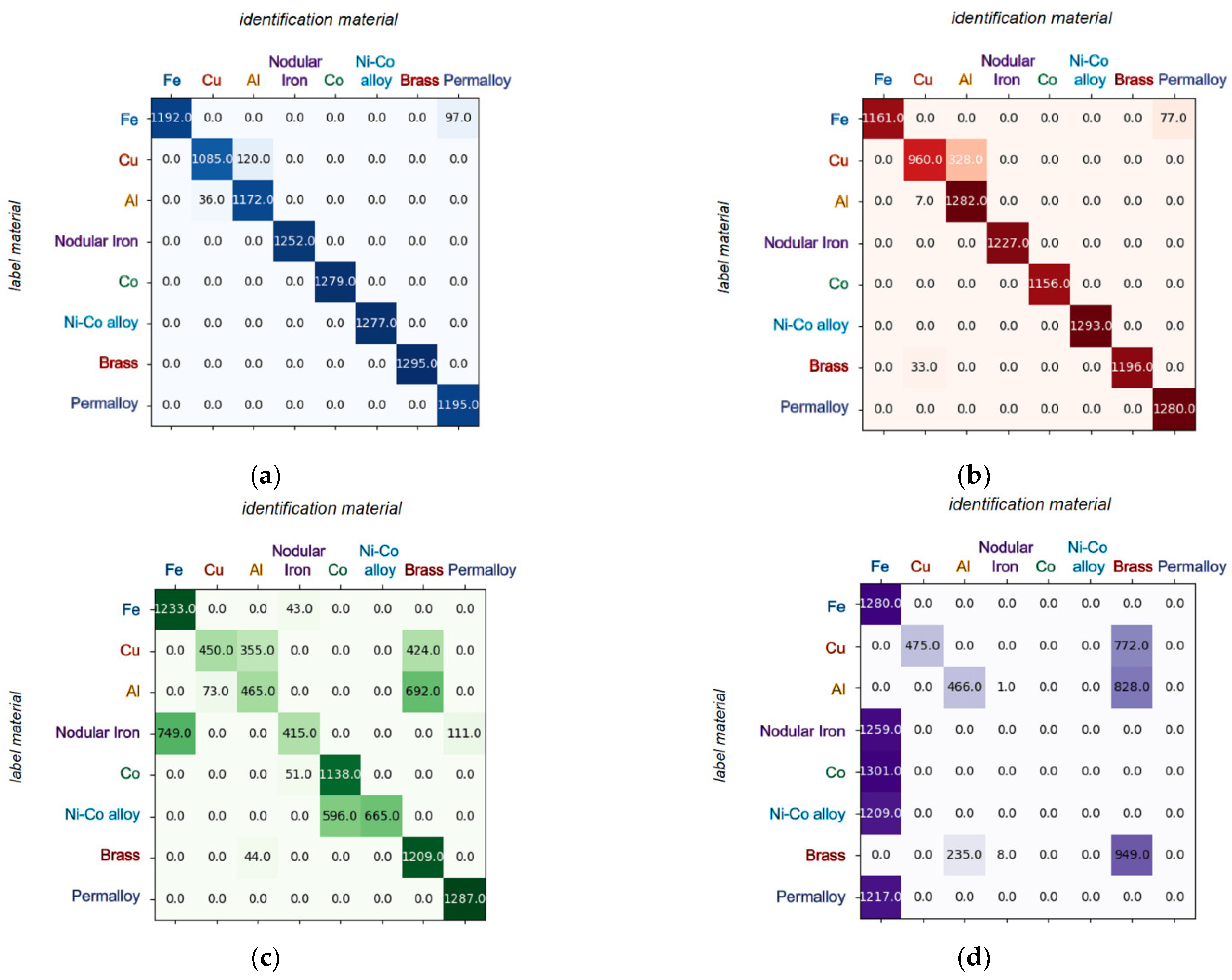
4.1. Confusion Matrix
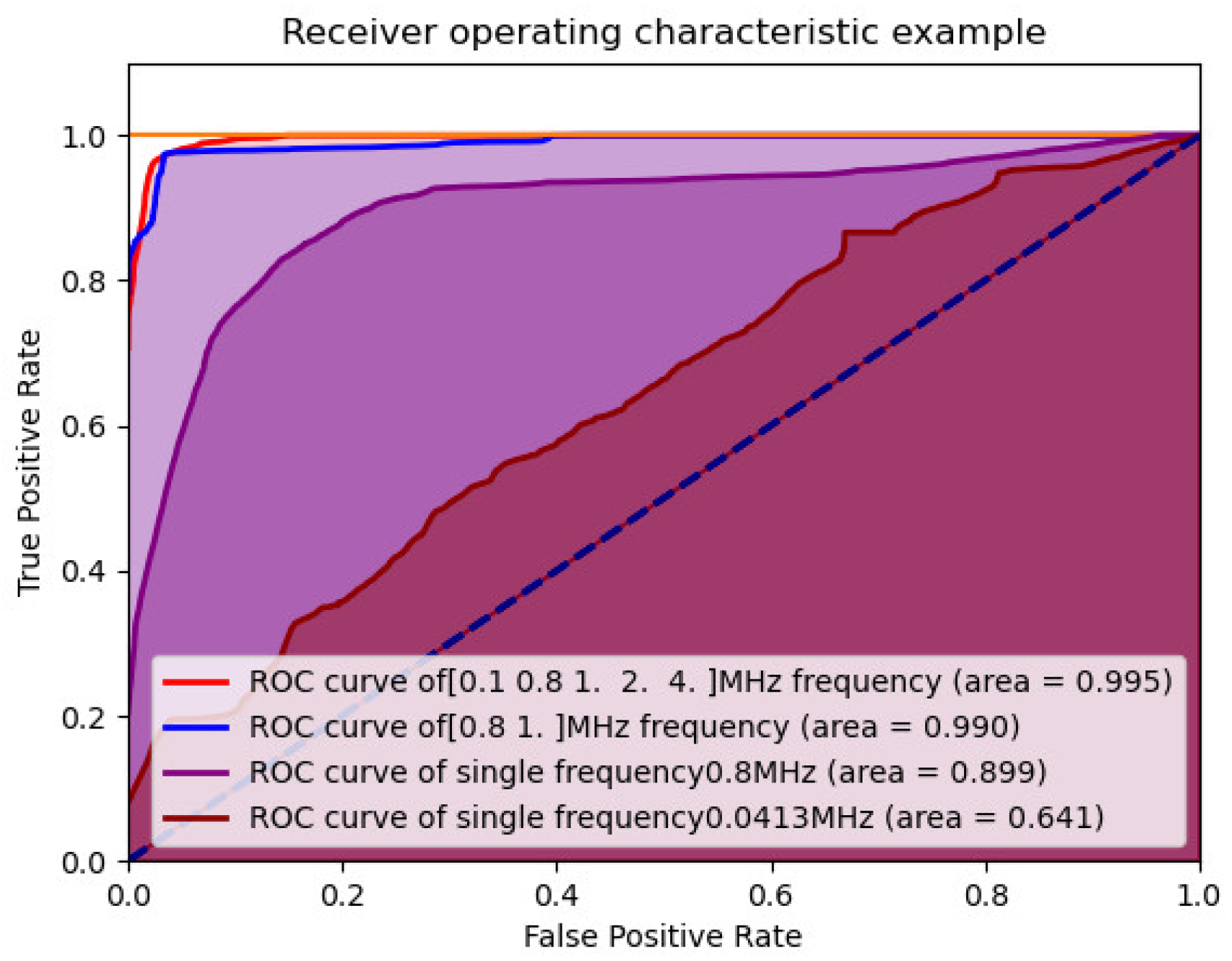
The ordinate of the confusion matrix represents the actual particle, and the abscissa represents the results of training. Thus, the element values in the matrix represent an intuitive correspondence between actual and predicted materials. Diagonal elements represent the number of samples correctly classified, and non-diagonal elements represent the number of samples wrongly classified [24,25].

4.2. ROC Curve

A more comprehensive indicator, namely the receiver operating characteristic (ROC) curve, was needed to evaluate the robustness of the identification results. The softmax layer output a list of probabilities directly, usually with the largest number in the list as a prediction. In the ROC curve, this rule is usually changed to take the value greater than the specified threshold as the result of the prediction. The rate that belongs to this class was denoted as the true positive rate (TPR); the rate that did not belong to this class was denoted as the false positive rate (FPR). By constantly adjusting the acceptance threshold, the results of the identification will also change. The corresponding TPR and FPR results can be plotted on a two-dimensional plane, and the curve obtained is the ROC curve. The area under the ROC curve (AUC) is often used as an intuitive indicator to measure the robustness of an identification. The AUC ranges from 0 to 1. When the AUC result is stable between 0.95 and 1, this indicates that the accuracy and robustness of the identification are excellent [26].

4.3. Identification Performance of Particle Material

Figure 5a,b represents the confusion matrix of the identification structure under multi-frequency measurement, whose identification results were much better than those of a single frequency in Figure 5c,d. Figure 5a shows the measurement results of five frequencies: 0.1, 0.8, 1, 2, and 4 MHz. Among them, identification errors were only evident between aluminum and copper, and between iron and permalloy. The proportion of misjudgment was less than 3%. The recall of Fe, Cu and Al were, respectively, 92.5%, 90%, and 97%, and other materials’ were 100%. The precision value of Cu, Al and permalloy were, respectively, 96.8%, 90.7%, and 92.5%, and other materials’ were 100%. Figure 5b shows the measurement results of two frequencies: 0.8 and 1 MHz. Compared to Figure 5a, the error rate was slightly higher, but was still controlled below 5%. The recall and precision value were similarly ideal. In Figure 5c,d, the identification errors also appeared in several types of fixed errors, which were in good agreement with the conclusions in Section 2.3. In other words, only when the characteristics in the complex plane are linearly separable can the neural network accurately identify the particle material. It is concluded that obtaining more measurement data under multi-frequency measurement can effectively improve the accuracy of detection.
The identification results of 10,000 groups were analyzed in order to discuss them in more detail. The ROC curve was drawn in Figure 6.
In Figure 6, the identification accuracy of five frequencies (0.1, 0.8, 1, 2, and 4 MHz) was 98%, and the ROC area also reached 0.995, which was far better than any one of these frequencies. Although both 41.3 kHz and 0.8 MHz are single frequencies, the identification results of 0.8 MHz were superior to 41.3 kHz. Compared with the results in Figure 5d, it can be seen that the identification results at 41.3 kHz were limited for the identification of the eight particles presented in this paper.
However, this does not mean that 41.3 kHz is unsuitable for particle detection. On the contrary, this frequency may be suitable for distinguishing particles of other materials. Particles of different materials have different conductivity and permeability, so they have different impedance results. Based on this consideration, the results of particle identification pre-training have more application value. This method can be used to find suitable frequencies or frequency combinations for particle identification before the design of circuits in practical engineering.
In addition, the accuracy of two frequencies (0.8 and 1 MHz) can reach 95%, which is basically close to five frequencies. In circuits, frequency is one of the main indexes when designing filters and other modules. Considering that obtaining impedance results at more frequencies will increase the cost of detection, detection at these two frequencies has greater application potential.

4.4. Identification Performance of Particle Size

After material identification was completed, particle size identification was carried out. A total of 30,000 training iterations were performed, respectively, at five frequencies for a fully connected network, two frequencies for a fully connected network, and two frequencies for neural network branches. The trained batch capacity was 1000. The confusion matrix and ROC curve are shown in Figure 7.
The particles wee evenly distributed within a given range of particle sizes, but the identification of particle sizes was not uniform, and the number of test samples with larger particle sizes was higher. This was acceptable for this study. The reasons for this are as follows: although the sample was uneven, it was sufficient that identification performance will not be significantly impaired. In addition, the particle size distribution generated in practical engineering may not have been uniform, and the distribution of pre-training data can be modified according to the actual situation.
By comparison of Figure 7a–c, identification errors were mostly concentrated between two adjacent size categories. In other words, particles whose size was at the class boundary tended to be mistakenly assigned to adjacent classes because of added noise.
In Figure 7c, the recall of 6~14 μ m , 14~21 μ m , 21~38 μ m , 38~70 μ m , and >70 μ m were, respectively, 98.3%, 98.2%, 100%, 99.4% and 95.4%. The precision value of 6~14 μ m , 14~21 μ m , 21~38 μ m , 38~70 μ m , and >70 μ m were, respectively, 85.1%, 99.3%, 98.4%, 97.6%, and 99.6%. By comparing the identification performance of the single network branch and the whole neural network in Figure 7, the identification accuracy of the neural network was seen to have greatly improved, reaching more than 95%. The area under the ROC curve also reached more than 0.993. It can also be seen that tree neural network can more easily obtain stronger fitting ability than other forms of single network branch.
By comparing the red line and the blue line in Figure 7d, under the same training times, the particle size identification at five frequencies was inferior to that of two frequencies, which is contrary to logical sense. The particle size identification at five frequencies requires more training parameters, but the actual training times were limited. Thus, the performance was not as good as that of the fully connected network at two frequencies. In other words, as available frequency components increased, a simple fully connected network was no longer appropriate and additional measures need to be taken to reduce the training parameters. For example, feature engineering such as principal component analysis (PCA) and dimension reduction can be performed before frequencies are input.

5. Conclusions

In this paper, a neural network particle identification algorithm with an autoencoder and pre-training mechanism was proposed for the characteristics of small particle identification samples and large differences among different sensors. In pre-training, the particle material identification accuracy rate achieved 98% and the size identification accuracy rate achieved 95%. The pre-training mechanism was based on the magnetization theory of metal particles in a magnetic field to enable database amplification, which avoids the problem of the high cost of particle sample acquisition. The autoencoder parameters were specifically used to characterize the measurement system parameters of different sensors, avoiding the high computational cost of training the full network for each sensor.
However, this study simply proposed ideal methods for second-stage training, not evaluating and discussing second-stage training identification performance. In the following research, our research group will make coils with excellent performance to complete this experiment.
In addition, we explored more research directions of metal particle detection through inductive sensors:
  • We established a frequency-finding scheme based on particle characteristics, which should be adapted to different engineering scenarios;
  • We confirmed that 0.8 MHz and 1 MHz are suitable for two-frequency measurement, which lays a theoretical foundation for the numerical selection of a subsequent multi-frequency measurement sensor.

Author Contributions

Methodology, X.Z. and H.Z.; software and validation, Y.C., G.H. and B.X.; writing—original draft preparation, Y.C. All authors have read and agreed to the published version of the manuscript.

Funding

Shandong Provincial Key Research and Development Plan (Grant No. 2021CXGC010702), National Natural Science Foundation of China (Grant No. 51909047), and National Key R&D Program of China (Grant No. 2019YFB1705302).

Institutional Review Board Statement

Not applicable.

Informed Consent Statement

Not applicable.

Data Availability Statement

Not applicable.

Conflicts of Interest

The authors declare no conflict of interest.

References

  1. Teng, H.; Zhang, H.; Liu, E.; Zeng, L.; Chen, H.; Bo, Z. New Method of Measuring Moisture Content in Marine Hydraulic Oil. Ship Eng. 2017, 39, 83–87. [Google Scholar]
  2. Zhang, H.; Zhang, X.; Guo, L.; Zhang, Y.; Sun, Y. Design of the microfluidic chip of oil detection. Appl. Mech. Mater. 2013, 34, 762–776. [Google Scholar] [CrossRef]
  3. Zhang, X. Study on Metal Particle Magnetization in Harmonic Field and Mechanism of Microfuidic Oil Detection; Dalian Maritime University: Dalian, China, 2014. [Google Scholar]
  4. Vasquez, S.; Kinnaert, M.; Pintelon, R. Active fault diagnosis on a hydraulic pitch system based on frequency-domain identification. IEEE Trans. Control Syst. Technol. 2019, 27, 663–678. [Google Scholar] [CrossRef]
  5. Shi, H.; Zhang, H.; Ma, L.; Rogers, F.; Zhao, X.; Zeng, L. An Impedance Debris Sensor Based on a High-Gradient Magnetic Field for High Sensitivity and High Throughput. IEEE Trans. Ind. Electron. 2021, 68, 5376–5384. [Google Scholar] [CrossRef]
  6. Sun, Y.; Yang, H.; Tong, H. Review of online detection for wear particles in lubricating oil of aviation engine. Chin. J. Sci. Instrum. 2017, 38, 1561–1569. [Google Scholar]
  7. Wang, J.; Maw, M.; Yu, X.; Dai, B.; Wang, G.; Jiang, Z. Applications and perspectives on microflfluidic technologies in ships and marine engineering: A review. Microfluid. Nanofluid. 2017, 21, 39. [Google Scholar] [CrossRef]
  8. Flanagan, I.; Jordan, J.; Whittington, H. Wear-debris detection and analysis techniques for lubricant based condition monitoring. J. Phys. E: Sci. Instrum. 1988, 21, 1011. [Google Scholar] [CrossRef]
  9. Sun, Y.; Jia, L.; Zeng, Z. Hyper-heuristic capacitance array method for multi-metal wear debris Detection. Sensors 2019, 19, 515. [Google Scholar] [CrossRef]
  10. Xu, C.; Zhang, P.; Wang, H.; Li, Y.; Lv, C. Ultrasonic echo waveshape features extraction based on QPSO-matching pursuit for online wear debris discrimination. Mech. Syst. Signal Process. 2015, 60–61, 301–315. [Google Scholar] [CrossRef]
  11. Paras, K.; Harish, H.; Atul, K. Online condition monitoring of misaligned meshing gears using wear debris and oil quality sensors. Ind. Lubr. Tribol. 2018, 70, 645–655. [Google Scholar]
  12. Iwai, Y.; Honda, T.; Miyajima, T.; Yoshinaga, S.; Higashi, M.; Fuwa, Y. Quantitative estimation of wear amounts by real time measurement of wear debris in lubricating oil. Tribol. Int. 2010, 43, 388–394. [Google Scholar] [CrossRef]
  13. Du, L.; Zhe, J. A high throughput inductive pulse sensor for online oil debris monitoring. Tribol. Int. 2011, 44, 175–179. [Google Scholar] [CrossRef]
  14. Zhang, X.; Zeng, L.; Zhang, H.; Huang, S. Magnetization Model and Detection Mechanism of a Microparticle in a Harmonic Magnetic Field. IEEE/ASME Trans. Mechatron. 2019, 24, 1882–1892. [Google Scholar] [CrossRef]
  15. NIST. SRM Order Request System SRM 2806b—Medium Test Dust (MTD) in Hydraulic Fluid [EB/OL]. Available online: https://www.sigmaaldrich.com/RS/en/product/sial/nist2806b?gclid=CjwKCAiAr4GgBhBFEiwAgwORrd7p80AXn_-qoStcBaSdDcIWYicslCP1qetrIFVv3UnlKMPB1ik9PBoC49IQAvD_BwE&gclsrc=aw.ds (accessed on 16 May 2022).
  16. Li, Y.; Yu, C.; Xue, B.; Zhang, H.; Zhang, X. A double lock-in amplifier circuit for complex domain signal detection of particles in oil. IEEE Trans. Instrum. Meas. 2021, 71, 3503710. [Google Scholar] [CrossRef]
  17. Samson, S.; Basri, M.; Fard Masoumi, H.R.; Abdul Malek, E.; Abedi Karjiban, R. An artificial neural network-based analysis of the factors controlling particle size in a virgin coconut oil-based nanoemulsion system containing copper peptide. PLoS ONE 2016, 11, e0157737. [Google Scholar] [CrossRef]
  18. Kumar, A.; Vishwakarma, A.; Bajaj, V. CRCCN-Net: Automated framework for classification of colorectal tissue using histopathological images. Biomed. Signal Process. Control 2023, 79, 104172. [Google Scholar] [CrossRef]
  19. Shinde, K.; Kayte, C.N. Fingerprint Recognition Based on Deep Learning Pre-Train with Our Best CNN Model for Person Identification. Electrochem. Soc. Trans. 2022, 107, 2209. [Google Scholar] [CrossRef]
  20. Simonyan, K.; Zisserman, A. Very Deep Convolutional Networks for Large-Scale Image Recognition. In Proceedings of the 3rd International Conference on Learning Representations, ICLR 2015—Conference Track Proceedings, International Conference on Learning Representations, ICLR, San Diego, CA, USA, 7–9 May 2015. [Google Scholar]
  21. Liu, J. Optimal Design and Analysis of Intelligent Vehicle Suspension System Based on ADAMS and Artificial Intelligence Algorithms. J. Phys. Conf. Ser. 2021, 2074, 012023. [Google Scholar] [CrossRef]
  22. Liu, B.; Yuan, P.; Wang, M.; Bi, C.; Liu, C.; Li, X. Optimal Design of High-Voltage Disconnecting Switch Drive System Based on ADAMS and Particle Swarm Optimization Algorithm. Mathematics 2021, 9, 1049. [Google Scholar] [CrossRef]
  23. Gu, Y.; Zhu, Y. Adams predictor–corrector method for solving uncertain differential equation. Comput. Appl. Math. 2021, 40, 61. [Google Scholar] [CrossRef]
  24. Mi, A.; Zhang, P. A method of classifier selection based on confusion matrix. J. Henan Polytech. Univ. (Nat. Sci.) 2017, 36, 116–121. [Google Scholar]
  25. Zhang, K.; Su, H.; Dou, Y. A new multi-classification task accuracy evaluation method based on confusion matrix. Comput. Eng. Sci. 2021, 43, 1910–1919. [Google Scholar]
  26. Victoria, M.; Antonio, M.; Alfonso, O.; Eduardo, L. Optimization of the area under the ROC curve using neural network supervectors for text-dependent speaker verification. Comput. Speech Lang. 2020, 63, 101078. [Google Scholar]
Figure 1. The principle of particle signal generation and signal characteristics.
Jmse 11 00541 g001
Figure 2. Characteristic curves of particle signals in a complex plane. (a) Frequency = 41.3 kHz; (b) frequency = 100 kHz; (c) frequency = 1 MHz; (d) frequency = 2 MHz.
Jmse 11 00541 g002
Figure 3. Particle identification neural network structure.
Jmse 11 00541 g003
Figure 4. Stages of training and identification.
Jmse 11 00541 g004
Figure 5. Confusion matrix for performance analysis of particle material identification at different frequency combinations. (a) Frequency = 0.1, 0.8, 1, 2, and 4 MHz; (b) frequency = 0.8 and 1 MHz; (c) frequency = 0.8 MHz; (d) frequency = 41.3 kHz.
Jmse 11 00541 g005
Figure 6. ROC curve for performance analysis of particle material identification at different frequency combinations.
Jmse 11 00541 g006
Figure 7. Confusion matrix and ROC curve for performance analysis of particle size identification at different frequency combinations. (a) Frequency = 0.1, 0.8, 1, 2, and 4 MHz, single neural network identification results; (b) frequency = 0.8, 1 MHz, single neural network identification results; (c) frequency = 0.8, 1 MHz, tree neural networks’ identification results; (d) ROC curves corresponding to (a), (b), and (c).
Jmse 11 00541 g007
Table 1. Common particle detection methods and their advantages and disadvantages.
Detection MethodsPrinciplesAdvantagesDisadvantages
Inductance Detection MethodUsing the magnetization and eddy current effect of oil metal particles under the action of the coil magnetic field to change the field, and then change coil inductance or voltage, according to the change in coil inductance or voltage detection.Ferromagnetic and non-ferromagnetic particles can be distinguished;
Not affected by cleanliness
Particles are indistinguishable when they are aliased
Capacitance Detection MethodMetal particles can be measured by using the change in oil capacitance.Metal and non-metal particles can be distinguished;
High sensitivity;
Not affected by cleanliness
The measurement accuracy is easily affected by the acid value and water content of oil;
Ferromagnetic and non-ferromagnetic particles cannot be distinguished
Ultrasonic Detection MethodWhen the ultrasonic wave acts on the particles in the oil, the particles will scatter or reflect the sound wave, attenuating the ultrasonic wave. Information about the size of the oil particles can be obtained by measuring the attenuation degree and amplitude of the echo.The size of metal particles can be estimated;
Not affected by cleanliness or air bubbles
The particle material cannot be judged
Image Detection MethodAn image of the pollutant in the fluid is obtained by microscope imaging technology, and the particle size and material property information are rapidly measured using image processing technology.The morphology and size of particles can be judged;
The particle material can be roughly judged
It is difficult to achieve both high precision and real-time performance;
Will be affected by cleanliness;
The particle material cannot be judged accurately;
Optical MethodInformation about the metal particles is obtained by measuring the light transmittance of oil.High sensitivityThe particle material cannot be judged;
Will be affected by cleanliness
Table 2. Conductivity and permeability of metal particles.
MaterialConductivity, (Siemens/m)Permeability, (H/m)
Fe 1.04 × 10 7 6.3 × 10 3
Cu 5.98 × 10 7 1.256629 × 10 6
Al 3.5 × 10 7 1.256665 × 10 6
Nodular Iron 1.370588 × 10 6 4.01858377 × 10 4
Co 1.1 × 10 7 5.735987 × 10 5
Ni-Co alloy 1.99862 × 10 7 8.269203 × 10 6
Brass 1.6744 × 10 7 1.256642 × 10 6
Permalloy 2.5 × 10 6 5.02654824 × 10 2
Table 3. Dataset for training and test.
DatasetFunction of DatasetFrequencySize of Dataset
Dataset 1training0.1, 0.8, 1, 2 and 4 MHz40,000
Dataset 2test0.1, 0.8, 1, 2 and 4 MHz10,000
Dataset 3training0.8 and 1 MHz40,000
Dataset 4test0.8 and 1 MHz10,000
Dataset 5training0.8 MHz40,000
Dataset 6test0.8 MHz10,000
Dataset 7training4.13 kHz40,000
Dataset 8test4.13 kHz10,000
Disclaimer/Publisher’s Note: The statements, opinions and data contained in all publications are solely those of the individual author(s) and contributor(s) and not of MDPI and/or the editor(s). MDPI and/or the editor(s) disclaim responsibility for any injury to people or property resulting from any ideas, methods, instructions or products referred to in the content.

