Article

Semi-Active Heave Compensation for a 600-Meter Hydraulic Salvaging Claw System with Ship Motion Prediction via LSTM Neural Networks

1
National Center for International Research of Subsea Engineering Technology and Equipment, Dalian Maritime University, Dalian 116026, China
2
Liaoning Province Key Laboratory Rescue & Salvage Engineering, Dalian Maritime University, Dalian 116000, China
*
Authors to whom correspondence should be addressed.
J. Mar. Sci. Eng. 2023, 11(5), 998; https://doi.org/10.3390/jmse11050998
Submission received: 19 April 2023 / Revised: 2 May 2023 / Accepted: 6 May 2023 / Published: 8 May 2023
(This article belongs to the Special Issue Technology and Equipment for Underwater Robots)

Abstract

:
Efficiently salvaging shipwrecks is of the utmost importance for safeguarding shipping safety and preserving the marine ecosystem. However, traditional methods find it difficult to salvage shipwrecks in deep water. This article presents a novel salvage technology that involves multiple hydraulic claws for directly catching and lifting a 2500-ton shipwreck at 600 m depth. To ensure lifting stability, a semi-active heave compensation (SAHC) system was employed for each lifter to mitigate the effects of sea waves. However, the response delays arising from the hydraulic, control, and filtering systems resist the heave compensation performance. Predicting the barge motion to mitigate measuring and filtering delays and achieve leading compensation is necessary for the salvage. Therefore, a multivariate long short-term memory (LSTM) based neural network was trained to forecast the barge’s heave and pitch motions, exhibiting satisfactory results for the next 5 s. According to the results of numerical simulations, the proposed LSTM-based motion predictive SAHC system demonstrates remarkable effectiveness in compensating for shipwreck motion.

1. Introduction

Nowadays, the demand for resources has led to a rapid expansion in both marine trade and scientific exploration, resulting in the construction of larger and more numerous vessels and offshore facilities. Unfortunately, it has also led to a significant increase in serious shipping incidents, with approximately 1000 such incidents occurring each year, which poses a threat not only to the marine ecosystem but also to the safe navigation of other vessels [1]. Therefore, removing these wrecks as quickly as possible is crucial to mitigate their impact on the environment and marine transportation.
Shipwrecks in shallow regions can be salvaged through traditional methods, including reestablishing buoyancy by attaching salvage pontoons around the hull and draining water from closed cabins or providing extra lifting force by floating cranes [2]. These methods, however, have obvious flaws. For instance, severely damaged shipwrecks cannot be drained to the extent necessary to achieve appropriate buoyancy, and fragile structures are also challenging to hoist using a floating crane. Furthermore, the majority of mono-hull or sheer-leg floating cranes in use currently lack the lifting capacity necessary to handle large shipwrecks weighing more than 10,000 tons [3]. For larger shipwrecks, a salvage technique named twin-barge synchronous lifting can be used. China’s Shanghai Salvage Bureau successfully salvaged the integral Korean M.V. Sewol from a 44 m depth by using the technique in 2017, with an 11,000-ton maximum lifting capability [4]. It used two barges spread across the water on either side of the shipwreck to share the load and installed 66 hydraulic strand jacks on them to provide lifting force. To cope with the sea-wave impacts, each hydraulic lifter also used a passive heave compensator (PHC) to reduce tension fluctuation on the slings [5]. Zhang et al. in-depth analyzed the performance of this salvage structure and revealed the effect of applying PHCs [6]. Compared with the traditional method, the twin-barge synchronous lifting has a significantly larger carrying capacity and better load stability for shallow regions. In contrast, however, deep water shipwreck salvage is a more challenging problem that needs to be solved.
Salvaging shipwrecks in deep water faces many difficulties. A significant challenge is the requirement for divers’ intervention, which is limited by the depth and duration of the diving work. For example, the salvage of the Russian submarine Kursk, which sank in 100 m of seawater with a weight of approximately 9500 tons, required a salvage barge and 26 lifting jacks. To attach lifting slings at that depth, divers had to dive and drill a total of 26 connecting holes on the wreck surface [7]. This project took approximately five months and required a significant amount of funding. Therefore, developing a large claw system that can catch the shipwreck mechanically, and without the need for divers, would be an efficient and convenient solution for deep salvage. A historical case that used a similar technique was recovering the Soviet submarine K-129 from the Pacific Ocean floor in 1974, about which detailed information was provided by Polmar and White [8]. Simply put, the U.S. government developed a massive mechanical salvage cradle to secretly recover the K-129 submarine. The cradle consisted of an integrated framework that could support the submarine, hydraulic claws to secure it, and hydraulic legs to pull it from the seabed soil. The project cost USD 500 million, which is roughly equivalent to the effort it took to put a man on the moon [9]. However, during the lifting process, one of the claws snapped under the weight, resulting in only part of the submarine being recovered [10]. There could be multiple reasons for the claw’s failure, such as insufficient structural strength or uneven weight distribution. While this attempt at deep-sea salvage was impressive, it also highlighted the fact that an integrated claw structure is overly complex and can result in unpredictable failures. Therefore, the claw salvage system should be designed as separate structures, with each claw functioning as a single unit, allowing for the combination of multiple claws to catch and lift shipwrecks.
Another key factor that could improve deep-sea salvage is heave compensation technology, which was also critical to the success of the salvage case mentioned above. The salvaging vessel will experience six degrees of motion under the influence of harsh sea waves and winds, resulting in excessive tension fluctuations on the lifting slings. They can also lead to unstable shipwreck motion in multiple degrees of freedom (DOFs) and amplified effects. Heave compensation, widely applied in various marine engineering fields, can effectively decouple the load motion and tension fluctuation from the motion of the working vessel and improves operating efficiency and time windows [11]. There are three types of heave compensation: passive, active (AHC), and semi-active [12]. PHC is a type of passive mechanical system that is mainly composed of a load-bearing hydraulic cylinder and gas–liquid accumulators. It can absorb and buffer load force fluctuations like a hydraulic spring by compressing the gas inside the accumulator, and improve the amplitude–frequency characteristic of the system by reducing the lifting stiffness fundamentally. The studies by Hatleskog et al. and Ni et al. indicated that PHC is more suitable for compensating for high wave frequency far from its natural frequency [13,14]. The PHC systems for the synchronous strand jack lifting in the M.V. Sewol salvage project, proposed by Wang et al., ensured successful operation [15]. However, despite PHC’s simplicity and cost-effectiveness, its compensating effect is limited compared with AHC and SAHC.
AHC and SAHC include a complete hydraulic or electronic actuator and closed-loop control system. They can detect the motion of the working point by IMUs and control the actuator to directly compensate for it, resulting in excellent efficiency [16]. The primary drawback of AHC is that its actuation and power systems need to match the payload weight, which limits its load capacity. SAHC combines PHC and AHC to overcome these limitations, resulting in a structure that boasts both high load capacity and excellent compensating effects. Currently, high-precision compensators with large load capacities are primarily implemented using SAHC solutions. For example, Niu et al. presented an SAHC system for a 3000 m, 200-ton lifting winch, and full-scale experiments demonstrated a 92.9% displacement compensation efficiency [17]. Quan et al. performed a scale model test of an SAHC for deep-sea tethered ROV, the test results indicated that SAHC has better efficiency in dealing with load resonance at critical depth than PHC [18]. Moreover, many novel control algorithms were designed to enhance the performance of SAHC systems, such as the nonlinear controller by Do et al., the model-predictive controller by Woodacre et al., and the H infinity robust controller by Zhang et al. [19,20,21], etc. For safety and steady working, it is essential to apply SAHC in deep water claw salvage operations. However, electro-hydraulic systems will be subject to various delay factors, the most significant of which comes from measurement noise filtering. The hydraulic control systems’ frequency response and the uncertainty in the sea waves can also contribute a lot. There is a need to predict the vessel’s motion and implement advance heave compensation to make up for the system delays.
Based on theoretical differences, there are three distinct approaches for predicting ship motion: Kalman filtering, time series, and machine learning neural network [22]. Kalman filtering methods necessitate the accurate hydrodynamic model of the vessel, which limits their practical implementation [23,24]. Time-series methods are more suitable for engineering predictions, as they rely only on historical and current motion data of the vessel rather than its system model. Several time-series models, including the classic auto-regressive (AR) model, and its extensions such as auto-regressive moving average (ARMA) and auto-regressive integrated moving average (ARIMA), are widely used [25,26,27]. However, ship motion exhibits non-stationary and nonlinear features, which conflict with the assumptions of stationary and explicit relationships between input and output datasets [28]. Neural networks possess the ability to effectively fit nonlinear systems without prior knowledge and can also manage multi-input multi-output predictions. When compared to traditional feed-forward neural networks, recurrent neural networks (RNNs), particularly those represented by long short-term memory (LSTM), demonstrate superior performance in capturing correlations between input motion sequences [29,30]. The studies in predicting semi-submersible and FPSO motion based on LSTM neural network presented by Guo et al. showed very good performance [31,32,33].
In this paper, a multi-claw shipwreck salvaging system for 600 m deep water with LSTM-based motion predicting SAHCs is presented. The SAHCs aimed to achieve a stable shipwreck salvage process for deep water. The LSTM-based neural network was mainly used to predict the barge’s heave and pitch motions in the next few seconds and tackle time delays raised by hydraulic and noise filtering systems. In Section 2, the working principle of the salvage system are described, and each part is mathematically modeled. In addition, the barge’s heave and pitch motion data under nine different sea conditions are also obtained in Section 2 through hydrodynamic simulation, for network training and simulation inputting. In Section 3, the predictive neural network model is designed and tested for finding the best structure. Finally, numerical simulations based on mathematical models, including the shipwreck’s 2-DOF dynamic, lifting slings, SAHCs, and controller are carried out for validation and evaluation purposes in Section 4. From the simulation results, some key contributions could be drawn out:
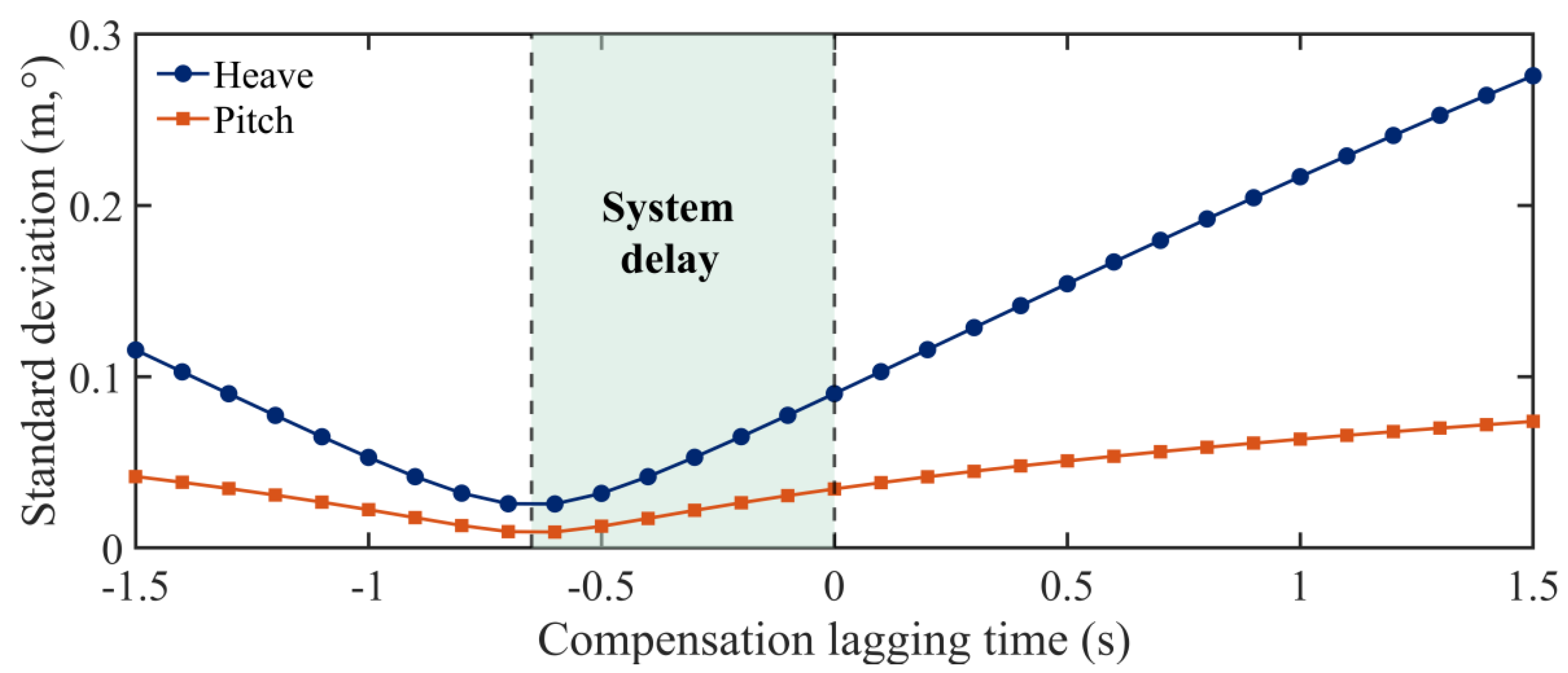
  • The system delays introduced by the hydraulic SAHC system and the noise filtering system seriously affect the compensation of the SAHCs to the shipwreck motion;
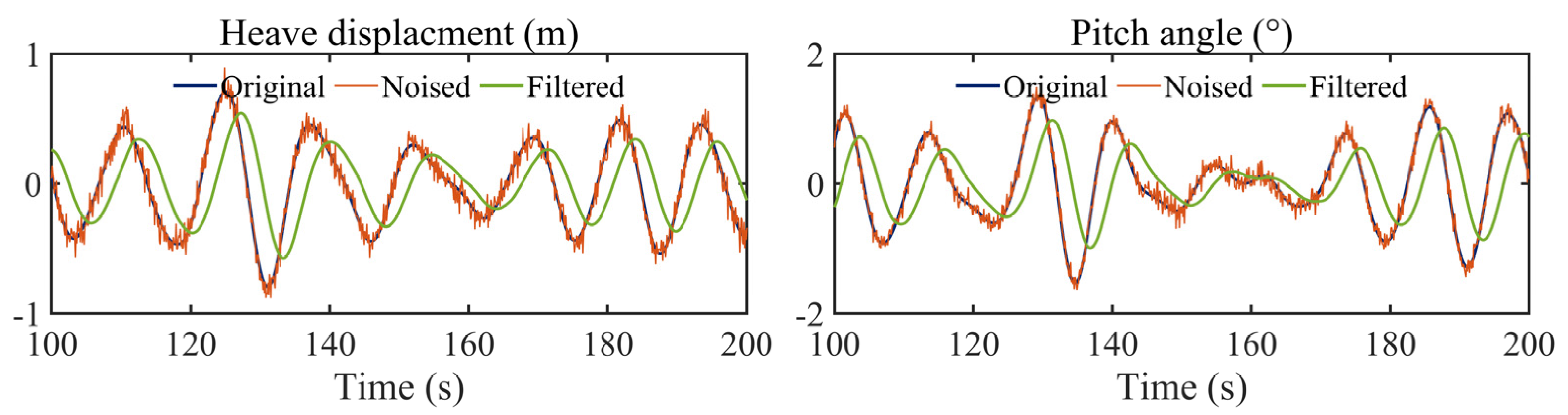
  • The delay introduced by noise filtering is commonly significant. In this study, the hydraulic control system alone has a delay of 0.6 s, which can reach more than 3 s when filtering is present;
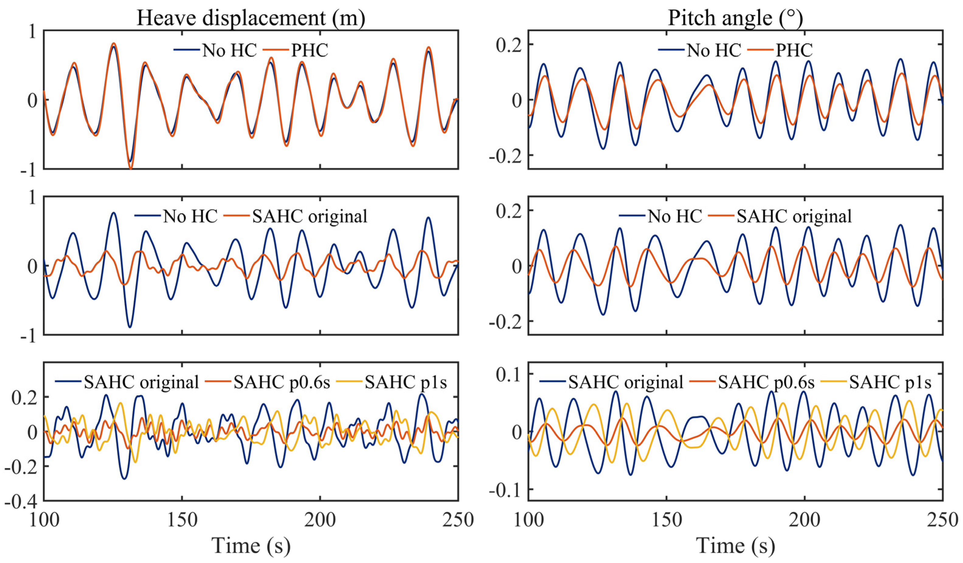
  • When facing deep water, the effect of PHC is insignificant because the lifting slings are already sufficiently flexible. However, applying SAHC can effectively reduce the shipwreck’s motion;
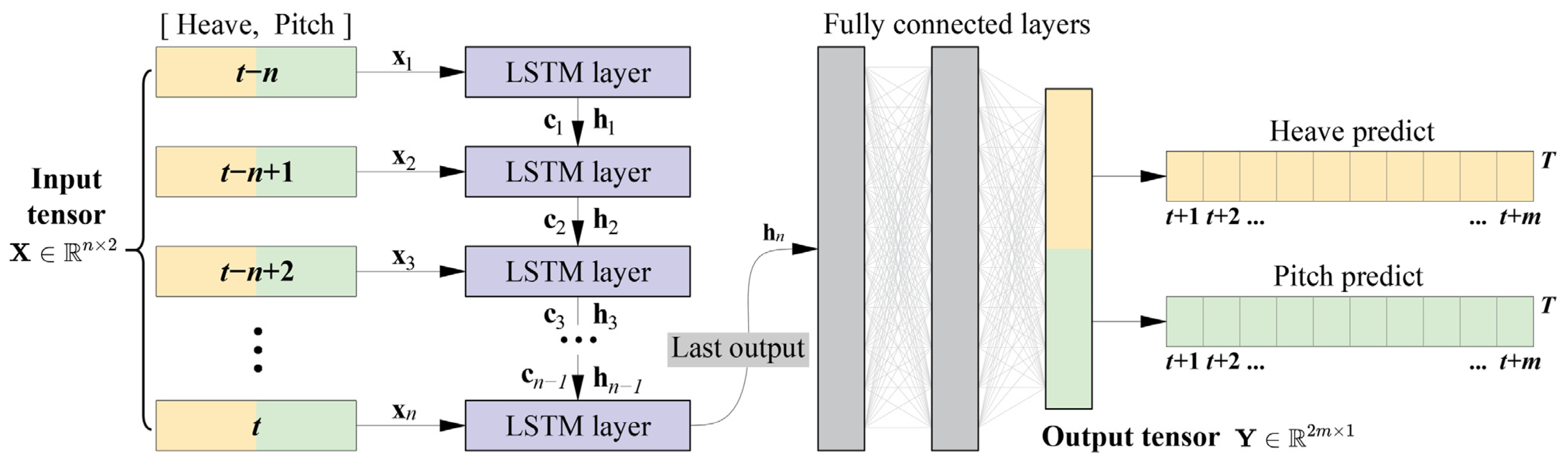
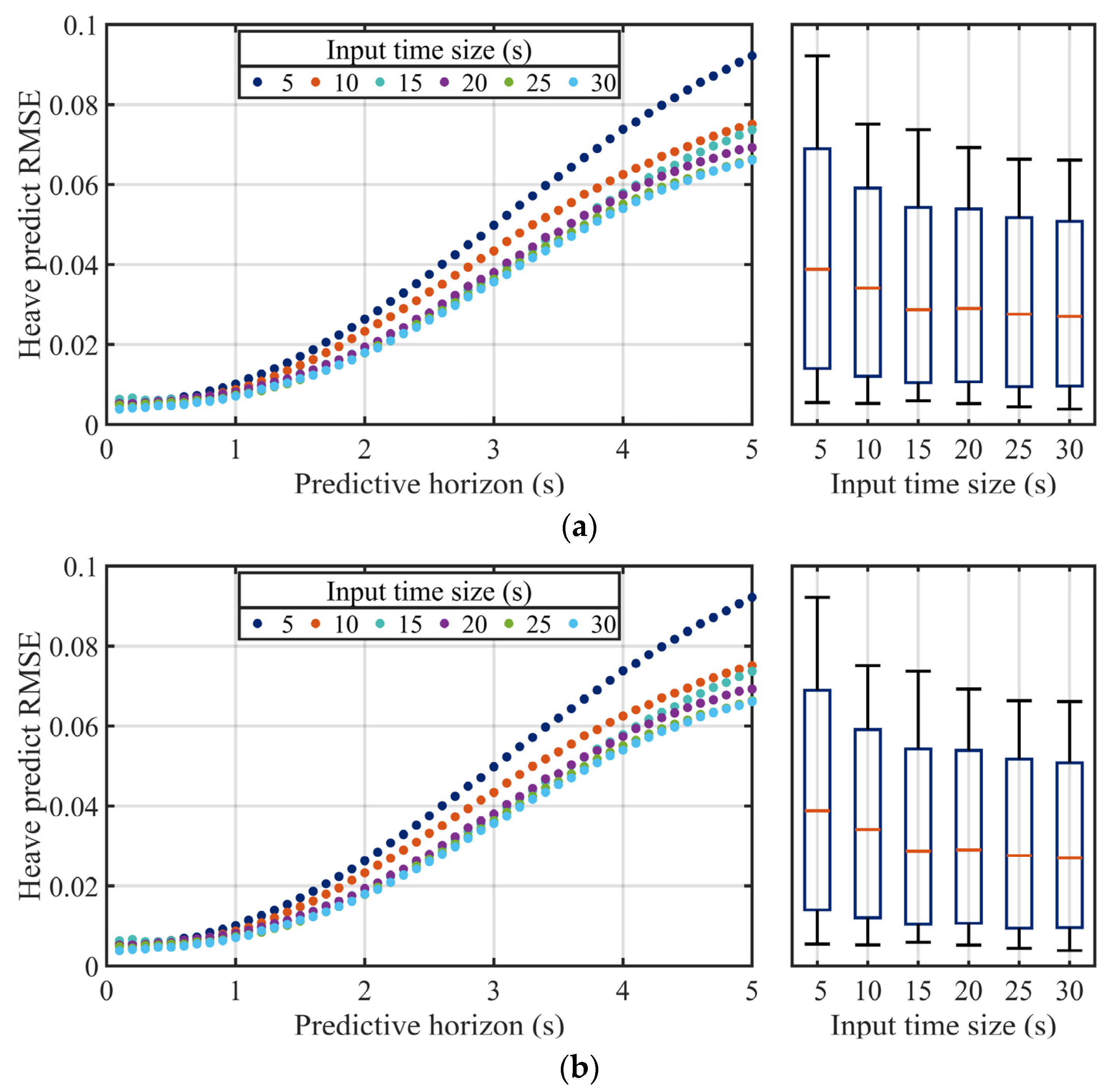
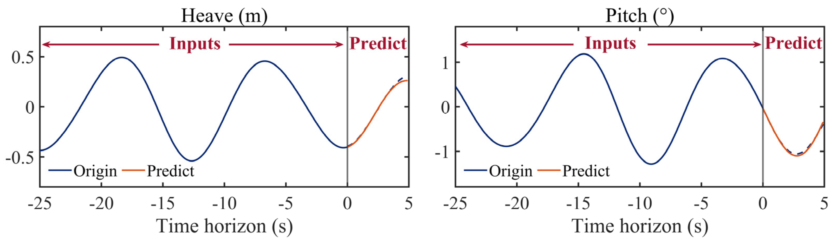
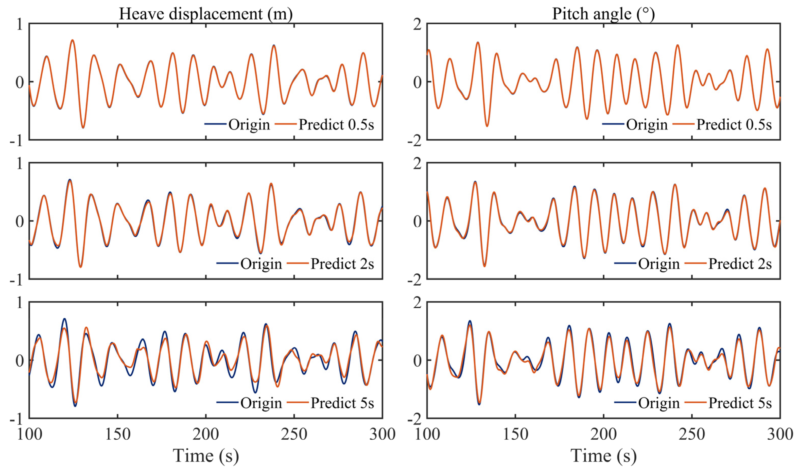
  • The proposed LSTM-based neural network can effectively predict the heave and pitch motions of the barge 5 s into the future based on the historical data, which is sufficient for the compensation system;
  • Motion prediction is necessary for systems lagged by noise filtering. SAHC without motion prediction is invalid when the noise exists.

2. System Modeling and Analysis

Establishing a mathematical model of a system is fundamental for conducting numerical simulations. This section provides a detailed description of the salvage system and establishes mathematical models for each component to facilitate subsequent numerical simulations. Additionally, this section includes a hydrodynamic analysis to obtain the motion data of the barge in various sea states. The resulting datasets will be used to train the neural network and serve as inputs for the numerical simulations in subsequent sections.

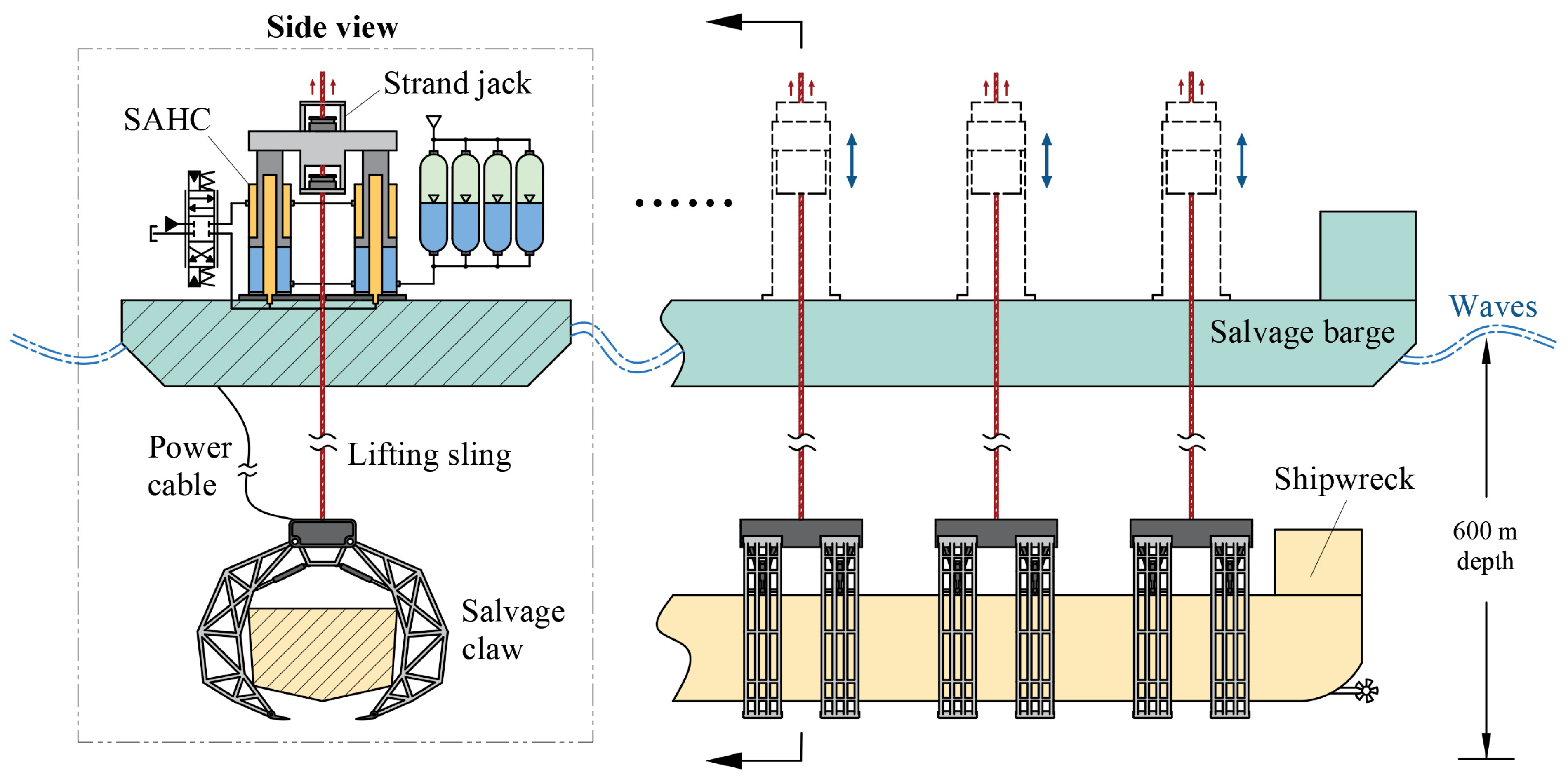
2.1. Claw Salvaging System

Figure 1 shows a schematic diagram of the multi-claw salvage system with SAHCs. The system consists of a salvage barge anchored to the water surface above the target shipwreck, deploying salvage claws at spaced intervals in the longitudinal direction. A synchronous strand jack lifting system, similar to that used in the salvage operations of the M.V. Sewol and the Kursk submarine, is used for shipwreck lifting [4,7]. This system comprises multiple hydraulic jacks that can work independently or be synchronized under computer control and is commonly used in the construction and marine industries [34]. However, this article mainly focuses on the predictive heave compensation system’s effect on a 600 m depth payload, disregarding the lifting effect and not considering the hydraulic jacks’ function.
As mentioned earlier, a vessel operating in sea waves will experience motion in six DOFs. Generally, the anchoring system can limit the salvage barge’s translational and rotational DOFs parallel to the water surface, such as surge, sway, and yaw, but it is unable to effectively restrict heave, roll, and pitch. Since the lifting devices on the barge are distributed longitudinally, the heave and pitch of the barge will cause a more significant vertical displacement at each lifter point. Therefore, an SAHC is installed between each strand jack and the barge deck. The compensation system will measure the real-time heave and pitch motions of the barge, calculate the vertical displacement of each lifting point, and control the SAHC cylinders to action. The cylinders will adjust their length to reverse the displacement caused by the heave and pitch motions, ensuring that the lifters remain stable during the salvaging process.
This study considers a shipwreck model with a submerged weight of 2500 tons and dimensions of 90 × 20 × 8 m (Lw × Bw × Hw). Nine salvage claws are symmetrically distributed along the longitudinal direction with a 10 m interval for salvage. Each claw weighs 240 tons and can provide a load capacity of 500 tons. Each lifting sling consists of eight 50 mm wire ropes, with a total weight of approximately 54 tons for the 600 m length. Therefore, the static load of each lifting sling is 518 tons, and the static load of each SAHC and lifter needs to be added to the sling weight, which is a total of 572 tons. To ensure safe operation, a salvage barge similar to the one used in the Sewol ferry salvage operation was chosen, which has dimensions of 140 × 56 × 8.88 m (Lb × Bb × Hb) and a displacement of 26,159 tons, with more specific parameters recorded in [4].

2.2. Mathematical Modeling

To perform a numerical simulation of the system, it is necessary to establish a mathematical model that can accurately describe the system’s dynamic and motion laws. The salvage system consists of two rigid bodies: the salvage barge and the shipwreck. In the simulation, the heave and pitch motions of the barge, which are obtained from the hydrodynamic analysis, will serve as the input signals for the numerical simulation. The motion of the shipwreck, sling tensions, and compensation systems will be iteratively calculated in response to barge motion inputs. The main focus of the simulation results will be the heave and pitch motions of the shipwreck and the tension variations in the slings.
Before establishing the mathematical model, certain simplifying assumptions should be considered:
  • Neglecting the dynamic effect of the shipwreck on the barge motion, since the barge has a larger inertia;
  • Assuming the shipwreck approximates a cuboid;
  • Considering the lifting sling as a linear spring model without banding and tilting;
  • Ideal gas with isothermal compression in the accumulators;
  • Only the heave and pitch motions are considered for both the barge and shipwreck.

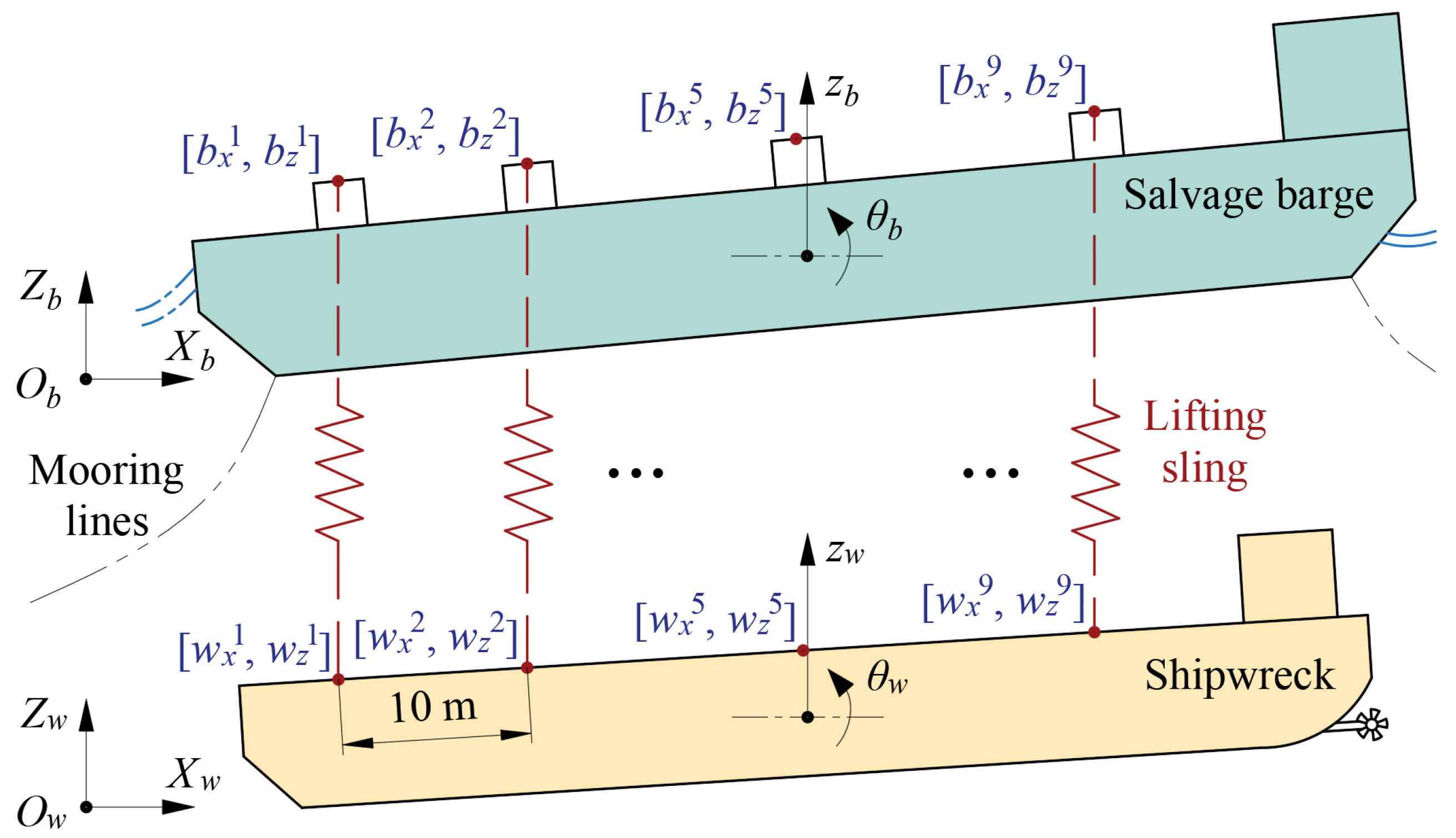
2.2.1. Barge–Shipwreck Motion Analysis

As shown in Figure 2, the barge and the shipwreck have their local coordinate systems, represented as XbObZb and XwOwZw, respectively. The heave displacements relate to the initial time and are denoted as zb(t) and zw(t) for the barge and the shipwreck, respectively. The pitch angles are denoted as θb(t) and θw(t), respectively. The origin positions of all lifter points in XbObZb and the positions of all lifted points in XwOwZw are assumed to be known and denoted as
B o = [ b x o 1 b x o 2 b x o i b z o 1 b z o 2 b z o i ] T   and   W o = [ w x o 1 w x o 2 w x o i w z o 1 w z o 2 w z o i ] T
where the superscript represents the number of the lifting sling, and the subscript represents the position component.
When the barge and shipwreck motions occur, the new positions can be calculated by
[ B W ] = [ B o 1 W o 1 ] [ Τ ( θ b , z b ) Τ ( θ w , z w ) ] [ 1 0 0 0 1 0 ] T
where T is the spatial transformation matrix. The term 1 = [1 1 … 1]T is one’s vector with i elements, whose purpose is to homogenize the position matrices Bo and Wo, allowing them to undergo heave transformations by T matrix. It should be emphasized that the vacancies in the matrix are all 0, with omission for brevity. The spatial transformation matrix T includes heave and pitch transformations and is a function of the heave displacement and pitch angle, that is
Τ ( θ , z ) = [ cos θ sin θ 0 sin θ cos θ 0 0 z 1 ]

2.2.2. Lifting Sling Tensions

Each lifting sling performs as a linear spring model, whose tension should relate to its elongation. Due to the assumption that lifting slings remain vertical, each elongation at any time only equals the differential between the vertical displacements of its top and lower end-point. Denoting the compensation displacements of SAHCs are xc = [xc1, xc2, …, xci]T, then the elongations of all slings can be expressed as
Δ l = Δ B z Δ W z + x c
where ΔBz are the vertical displacements of the points B related to its origin point Bo, and the same for ΔWz. They can be calculated by
[ Δ B z Δ W z ] = [ B B o W W o ] [ 0 1 ]
Then, the sling tensions are expressed as
F s = k s Δ l
where ks is the equivalent stiffness of a single lifting sling.

2.2.3. Shipwreck Heave and Pitch Dynamics
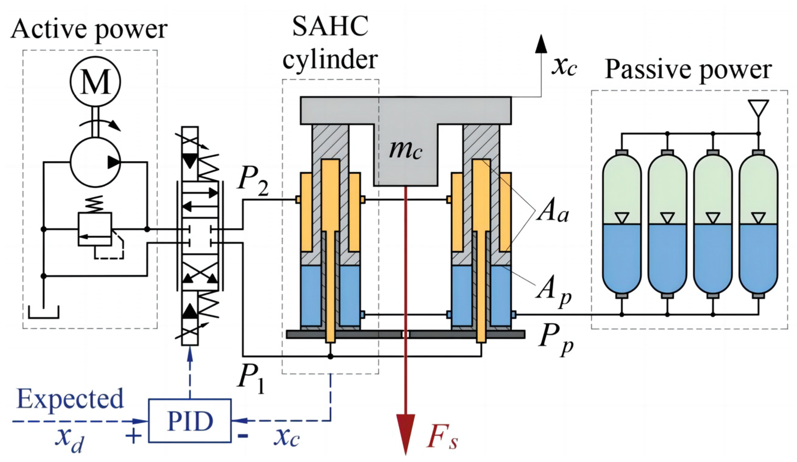
The shipwreck is subjected to four main forces: buoyancy, gravity, sling tensions, and water resistance. During the lifting process, uneven sling tensions will cause translational and rotational accelerations in the heave and pitch motions. Firstly, the dynamic equation describing the heave motion of the shipwreck can be given by
k a d d m w z ¨ w + D z z ˙ w | z ˙ w | = 1 T F s + F b m w g
where kadd is the additional mass factor, mw is the mass of the shipwreck, Dz is the drag coefficient, Fb is the buoyancy, and g is the acceleration due to gravity.
The drag force in the heave direction is proportional to the square of an object’s heave velocity. It also depends on the water density, ρsea, and the projected area perpendicular to the object’s velocity direction. In fluid mechanics, the drag force is mainly comprised of pressure drag resulting from the difference in pressure between the front and back of the object, and a portion of the friction drag from the sides. The drag coefficient is given by
D z = 0.5 C D ρ s e a L w B w cos θ w
where CD is a shape coefficient.
The dynamic equation describing the shipwreck’s pitch motion can be given as
k a d d I w θ ¨ w + D r θ ˙ w | θ ˙ w | = 1 T M s
where Iw is the moment of inertia for the pitch motion of the shipwreck, Dr is the drag torque of pitch motion, and Ms = [Ms1 Ms2Msi]T is the torque vector on the shipwreck’s rotation center caused by the sling tensions.
The sling tension torque can be expressed by
M s = W n x F s
where nx = [1 0]T is a normal vector along the x-axis, and ○ is the Hadamard product, which multiplies two vectors element-wise.
Since torque is related to both force and the length of the moment arm, the shipwreck will experience different values of drag torque at different turning radii. In order to calculate this, the total drag torque will be obtained through the integration of the drag torque at each turning radius. For an infinitesimal element of length dr located at a distance r from the center of the shipwreck’s pitch rotation, its normal velocity is
v = θ ˙ w r
Then, its normal drag force can be expressed as
d D = 0.5 C D ρ s e a v | v | ( d r B w )
By substituting the normal velocity, its drag torque can be expressed as
d M D = r d D = 0.5 C D ρ s e a θ ˙ w | θ ˙ w | B w r 3 d r
Finally, the pitch drag torque can be integrated as
M D = 2 0 L w / 2 d M D = 1 64 C D ρ s e a B w L w 4 θ ˙ w | θ ˙ w |
from which Dr = 1/64CDρseaBwLw4 can be obtained.

2.2.4. SAHC

A single SAHC system consists of two integrated cylinders for load bearing, an active hydraulic system with a 3-position 4-way proportional valve for continuous flow rate control, and a passive power system with multiple gas accumulators, as illustrated in Figure 3. The integrated cylinder has a compact structure with three isolated chambers, two active chambers with the same effective areas, and a passive chamber. The active chambers are linked to the proportional valve for active displacement control, while the passive chamber is connected to gas accumulators for payload bearing.
The hydraulic system as a whole is divided into a passive part and an active part. The working pressure of the passive chambers and accumulators is mainly generated by gas compression, which is caused by the displacement of the cylinder. According to Boyer’s law, that the state of an adiabatic gas can be expressed as P1V1n = P2V2n, the passive working pressure can be derived as
P p = P 0 ( V 0 V 0 + 2 A p x c ) n
where P0 is the initial pressure of the accumulators, V0 is the total gas volume in the accumulators, Ap is the effective area of the passive chamber, and n is the adiabatic index.
The initial pressure of the accumulators should support the combined weight of the shipwreck mw and the lifting sling ms, which is
P 0 = ( m w + m s ) g
The active part functions as a cylinder system controlled by a proportional valve, enabling continuous regulation of the speed and motion direction of the cylinder by adjusting the valve opening. The area of each active chamber is denoted as Aa, and the oil pressure and flow rate of the inlet chambers are denoted as P1 and q1, respectively. The oil pressure and flow rate of the outlet chambers are denoted as P2 and q2, respectively. The positive direction of the flow rate is defined as the flow direction when cylinder extension (xc > 0). Then, considering the oil compression, the flow continuity equations of two active chambers can be expressed as
q 1 = 2 ( A a x ˙ c + V 1 β e P ˙ 1 )   and   q 2 = 2 ( A a x ˙ c V 2 β e P ˙ 2 )
where V1 = V10 + Aaxc and V2 = V20Aaxc are the oil volumes of the inlet and outlet chambers, V10 = V20 are the initial oil volumes of the inlet and outlet chambers, and βe is the oil bulk modulus.
Additionally, the flow rates across the proportional valve are related to the valve opening xv, which can be expressed as
q 1 = C d ω x v 2 | P s P 1 | ρ o i l sgn ( P s P 1 )   and   q 2 = C d ω x v 2 | P 2 | ρ o i l sgn ( P 2 )
where Cd is the orifice flow coefficient, ω is the throttle area gradient, ρoil is the oil density, and sgn(·) is the sign function.
Since the response speed of the spool is significantly faster than the action frequency of the hydraulic system, the dynamic characteristics of the spool can be neglected. The pressures in the two chambers can be determined by solving a first-order nonlinear differential equation system that combines the continuity equations of the hydraulic cylinder and the flow equations of the valve, concerning the piston displacement xc and the valve opening xv. These equations can be solved iteratively in the numerical simulation.
Finally, the dynamic equation that describes the piston motion of the SAHC can be expressed as
m c x ¨ c + b c x ˙ c = 2 A a ( P 1 P 2 ) + 2 A p P p F s
where mc is the total mass of the piston and attachments, and bc is the damping coefficient of the compensator.
Afterward, the compensating displacements of all the SAHCs will continue to update the sling tensions, completing the closed loop of the numerical calculation.

2.3. Barge Motion Hydrodynamic Analysis

The objective of the hydrodynamic analysis is to generate time-series data of the salvage barge’s heave and pitch motions under various sea conditions. The majority of these data will be used to train a motion predictive LSTM neural network, while the remaining data will serve as input for the numerical simulation of the barge’s motion. Figure 4 illustrates the chosen sea conditions according to the actual wave scatter statistics and their dataset purposes, where the wave parameters are described by JONSWAP [35]. The sequence data for each sea condition will comprise 2000 s of time-series data for the barge’s heave and pitch motions, sampled at intervals of 0.1 s.
In the hydrodynamic analysis, only the head sea condition is applied, since we just focus on the heave and pitch motions of the barge. For simulated shipwreck weight, a static downward force equal to the shipwreck gravity is exerted under the barge. In addition, a four-point mooring system is also applied to keep the barge stable [36]. Other major parameters of the barge and the mooring system are listed in Table 1 below.
Figure 5 shows the response amplitude operators (RAOs) of the salvage barge’s motions in different wave periods, obtained through hydrodynamic analysis. It is observed that the pitch motion exhibits a peak value at around 12 s, indicating its significant influence during this wave period. Although time-domain motion figures can also be provided, due to their vast number only the figures of the testing set are presented in Figure 6.

3. LSTM-Based Barge Motion Prediction

The LSTM neural network is an upgraded version of the traditional recurrent neural network (RNN). Unlike feed-forward neural networks, the traditional RNN can utilize its previous step information as internal memory for the current network. This allows it to extract time features from the input sequence, making it more suitable for time-series prediction. Its parameter size is only related to the feature size of the sequential input data, but not the time length, giving it the advantage of allowing different sequential lengths in the same network. However, the information of the data far from now may be lost in the internal memory with each iteration, and problems such as gradient vanishing and exploding may occur during the backpropagation process, decreasing the accuracy and applicability of the traditional RNN. To address these issues, long short-term memory (LSTM) was proposed, with the key improvement being the addition of a memorization and forgetting mechanism in the recurrent processing.

3.1. LSTM-Based Motion Predictive Neural Network

The LSTM is a variant of RNN which has three tunable gates: the input gate, the forget gate, and the output gate [37]. As shown in Figure 7, the input gate, denoted by it, determines which information from the input should be added to the cell state, while the forget gate ft controls which information should be discarded from the cell state. The output gate ot regulates how the information in the cell state should affect the output at the next time step. With the cooperation of these three gates, the LSTM network can retain and forget the previous data information, and decide which information to add or output based on the current input data, thus better handling long-term dependencies in time series. The formulas of an LSTM cell are shown below:
i t = σ ( W x i x t + b x i + W h i h t 1 + b h i ) f t = σ ( W x f x t + b x f + W h f h t 1 + b h f ) g t = tanh ( W x g x t + b x g + W h g h t 1 + b h g ) o t = σ ( W x o x t + b x o + W h o h t 1 + b h o ) c t = f t c t 1 + i t g t h t = o t tanh ( c t )
where W and b are the weights and bias matrices of a network cell, respectively, σ(·) is the sigmoid active function, gt is the cell gate, ct is a recurrent cell state that is responsible for recording long-term relationships, and ht is the hidden state and also the cell output. For each W and b, the first subscript annotates the vector it multiplies, with x representing the input vector x and h representing the hidden state h. The second subscript indicates which gate it belongs to, including i (input gate), f (forget gate), g (cell gate), and o (output gate).
Figure 8 illustrates the structure of the proposed LSTM-based motion predictive neural network. For motion prediction, we expect the predictive neural network could accept the historical sequences of the barge’s heave and pitch motions, then output their predicted future sequences. Therefore, an LSTM recurrent layer aimed at inputting the sequential vectors of each step, containing one heave and one pitch datapoint, is first constructed in the network. The input size for the LSTM layer is n × 2, which represents two features in one recurrent step and a total of n input steps. Although the sequence length allowed by LSTM is arbitrary, only the equal length is used for training and testing in this paper. By repeatedly self-iterating, the LSTM layer fully extracts the dependent information of the motion sequences and gives the final step’s hidden state as the layer output, which is a vector with a length equal to the LSTM cell size. Then, containing past information, the layer output will pass three fully connected layers and be reshaped to an output vector combining the sequential predictions of the heave and pitch. For this paper, we set the predictive horizon as far as a fixed 5 s, meaning that the network outputs future sequential data of 50 points heave then 50 points pitch at one time (m = 50). By splicing the output tensor, the predictive motion sequences could be obtained.
The major layer parameters of the proposed network are listed in Table 2, where the size of the LSTM cell is 1024 and the sizes of the first two fully connected layers are 512. The size of the last fully connected layer is 100, which is used to reshape the output tensor. The trained process uses the Adam method with a decaying learning rate to ensure accuracy. The entire training set was shuffled into mini-batches and repeated training for 20 epochs, with an initial learning rate of 0.0001 and a decay of 0.4 times after every 4 epochs.

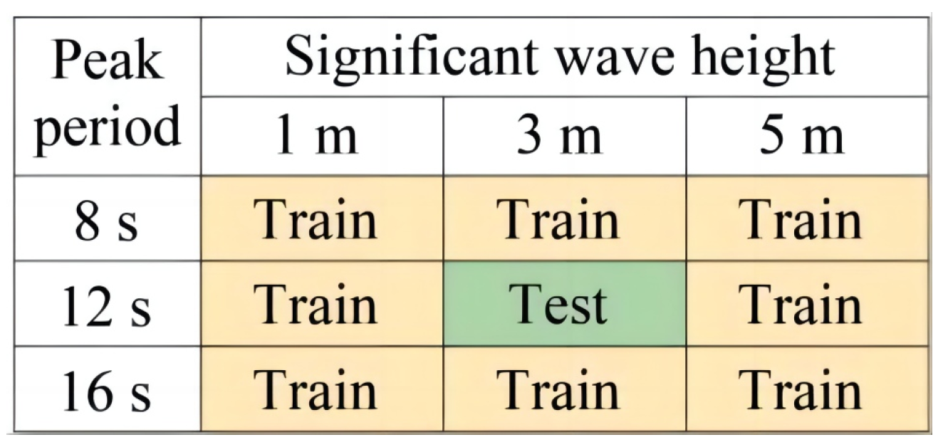
3.2. Network Training and Testing

The datasets used in the predictive neural network are shown in Figure 4, consisting of eight sequences for training and one for testing. The test set data is not used for training due to the difficulty in obtaining on-site sea state information during actual salvaging operations. The training sets are randomly shuffled and split into input and output tensor pairs. The output tensor size is fixed at 100 elements, with 50 elements of the sequential heave and 50 elements of the sequential pitch. To evaluate the effect of input tensor length, networks with varying lengths of input sequences are first trained and tested.
The root-mean-square error (RMSE) performance of the networks was evaluated and the results are presented in Figure 9. Each evaluation was averaged over multiple training sessions. The left side of the figure shows the predictive performance of the networks with different input time sizes for varying prediction horizons, while the right side displays the corresponding error box plots. It is expected that the prediction errors of all the networks increase with the prediction horizon. The best prediction performance for heave is achieved with the input time sizes of 25 s and 30 s, while the former is better for pitch prediction. Therefore, it can be concluded that an input time size of 25 s, which represents an input length of 250 points, is more suitable for improving the prediction accuracy of the proposed neural network.
After fixing the input length (n = 250) and the prediction length (m = 50), the predictive neural network is fully trained and the results of continuous motion prediction for the testing set are presented. Figure 10 displays the sequential input and prediction output curves at a specific moment, while Figure 11 shows the continuous rolling predictions for the barge’s heave and pitch, with prediction horizons of 0.5 s, 2 s, and 5 s. Although the 5 s prediction shows some deviations at the peaks compared to the ground-truth data, it is still considered acceptable.

4. Simulation Results and Analysis

In this section, the numerical simulation of the salvage system is implemented for testing the compensation and motion prediction performance. The involved numerical models were introduced in Section 2.2. The simulation parameters which have not yet been mentioned are listed in Table 3. Furthermore, the heave compensation system uses traditional PID controllers for position closed-loop control, which can ensure the basic dynamic tracking ability of the compensation cylinders.
The working process of the predictive compensation system can be summarized as follows: first, the heave and pitch signals of the barge are measured. Next, the LSTM-based neural network is used to predict the future heave and pitch values according to the historical sequential signals. Then, the predicted results are transformed into displacement compensation values for each SAHC through coordinate transformation. Finally, the controllers are ordered to perform the necessary compensation actions on the SAHCs.
It is important to reiterate that the purpose of barge motion prediction is to compensate for the hysteresis in the compensation system, which may arise from various factors such as the PID controller, hydraulic system response, dynamic characteristics of the salvage system, and filtering process of the motion measurements. However, we believe that the filtering process of the sensor has a greater impact. Therefore, in the following analysis, we will consider the effects of both situations, with and without measurement noise.

4.1. Influence of Lead/Lag Compensation

Before testing the effectiveness of predictive heave compensation, the time-delay characteristics of the SAHC system without motion prediction were analyzed. The simulation results are presented in Figure 12, which demonstrates the effect of changing the time position of the barge signal input to the SAHC system. A positive value on the horizontal axis indicates that the compensation amount lags behind the actual movement of the barge, and a negative value indicates that the compensation amount is ahead of the actual movement of the barge. By analyzing the standard deviation changes in the shipwreck motion in each corresponding case, it can be concluded that both the compensation lag and premature lead compensation can intensify the motion of the wreck. Furthermore, it was found that the minimum motion result was obtained at 0.6 s of lead compensation, rather than 0 s. This indicates that the system has a 0.6 s delay from the barge motion measurement to the SAHC’s displacement acting, highlighting the importance of motion prediction and advancing compensation.

4.2. Predictive Compensation without Measuring Noise

Based on the barge motion without noise pollution, this section simulates and compares the heave and pitch time-domain motions of the barge in different heave compensation modes: non-compensation, PHC mode, original SAHC mode without prediction, and SAHC mode with prediction. The results are displayed in Figure 13, from which the following conclusions can be drawn:
In the absence of heave compensation, the heave and pitch motions of the shipwreck are significant. Even with the passive mode, only the pitch motion is slightly weakened. This limited performance is primarily due to the reduced sling stiffness of the 600 m length, and cannot be further reduced by the PHCs.
Compared to the non-compensation condition, the original SAHC mode without motion prediction can significantly reduce both the heave and pitch motions of the shipwreck, with standard deviation (STD) decrements of about 67.59% and 53.77%, respectively. Furthermore, when motion predictions are applied, the motion STDs are further reduced by about 66.89% and 68%, with a 0.6 s prediction. However, when the prediction time is switched to 1 s, the motions become significant, which is consistent with the results shown in Figure 12.

4.3. Predictive Compensation with Measuring Noise

In this section, it is assumed that the motion signal of the barge is contaminated by white noise and should be filtered before being input into the predictive neural network. Therefore, a second-order low-pass filter is used to filter the motion signal, and its transfer function is given by
H ( s ) = ω n 2 s 2 + 2 ω n s + ω n 2
where ωn is the cut-off frequency, whose value is set as ωn = 0.8.
Figure 14 presents a comparison between the original data of the barge’s heave and pitch, the noisy data, and the filtered data. The filtering process introduces a delay of approximately 2.5 to 3 s to the original data. It should be noted that this delay can be further reduced by using a better filter, such as the Kalman filter.
The filtered data is input into the neural network for motion prediction, and the predicted result is used as the expected compensation amount of the SAHC system. The final simulation results are presented in Figure 15, which includes the curves for SAHC without heave compensation (as in Figure 13), the SAHC system without motion prediction, and the predictions for 1 s, 3 s, and 4 s.
The delay introduced by the filtering process and the presence of noise makes it difficult for the various SAHC systems to completely compensate for the motion of the wreck. However, it was found through simulations that the best compensation effect can be achieved when the prediction time is set to 3 s. If the prediction time is greater or less than this, the compensation effect will be reduced. At this prediction time, the standard deviations of the barge motion are reduced by 44.14% and 43.19% in heave and pitch, respectively, compared to the uncompensated case. This result is lower than the ideal noise-free situation shown in Figure 13, but it is more representative of the actual engineering situation, where noise is expected.

5. Conclusions

In this paper, a shipwreck salvaging system with multiple hydraulic claws, capable of operating at depths of up to 600 m, is proposed. This system incorporates SAHCs to ensure stable lifting operations. Additionally, a multivariate LSTM-based neural network is introduced for predictive compensation of barge motion. Through hydrodynamic analysis, heave and pitch motion sequences of the working barge in nine different sea conditions were obtained for neural network training and numerical simulation input. In the proposed neural network, the historical heave and pitch sequences of the barge were fed into the LSTM cell and reshaped by several fully connected layers to obtain future motion sequences. The testing results demonstrated that a historical sequential input of 25 s was the most suitable for the neural network to achieve a 5 s sequential prediction. Then, the performance of the SAHC system and the predictive neural network are tested through a numerical simulation based on the mathematical models described in Section 2. Based on the results in Section 4, the following conclusions could be drawn out:
  • Passive heave compensation has minimal effects on a shipwreck’s motion at this depth;
  • When the SAHCs are employed without motion prediction, the standard deviations of the shipwreck motion are significantly reduced, by 67.59% in heave and 53.77% in pitch;
  • In the absence of measurement noise, a 0.6 s predictive compensation to counter system delay further reduces shipwreck motion by 66.89% and 68% in heave and pitch, respectively, compared to the non-prediction case;
  • SAHCs without prediction exhibit poor compensation effects in the presence of noise pollution in barge motion measurement;
  • In such scenarios, a 3 s predictive compensation can achieve the best compensating performance, resulting in a reduction in shipwreck motion to 44.14% in heave and 43.19% in pitch.
These results underscore the indispensability of motion prediction in deep-sea shipwreck salvage operations and highlight the good performance of the proposed LSTM-based predictive neural network and SAHC system. In conclusion, the efficacy of the proposed predictive SAHC system for a 600 m multi-claw shipwreck salvaging system has been demonstrated, with potential implications for real-world engineering practices. Future endeavors will entail conducting factory tests in a laboratory wave pool to further validate the system’s capabilities. Furthermore, collecting more motion data from actual barges at sea, to enhance the motion predictive network’s reliability, is work that this paper did not address and will be incorporated into future research.

Author Contributions

Writing—original draft preparation, software, F.Z.; writing—review and editing, D.N. and H.T.; methodology, validation, J.H.; software, H.D.; investigation K.Z.; supervision, Y.G. All authors have read and agreed to the published version of the manuscript.

Funding

This work was carried out with the support of the National Nature Science Foundation of China (52075064, 51405054), and Fundamental Research Funds for the Central Universities.

Institutional Review Board Statement

Not applicable.

Informed Consent Statement

Not applicable.

Data Availability Statement

Not applicable.

Conflicts of Interest

The authors declare no conflict of interest.

References

  1. Gray, W. Raising titans: How do you salvage a mega-ship? New Sci. 2013, 220, 48–51. [Google Scholar] [CrossRef]
  2. Dean, M.S. Salvage operations. In Springer Handbook of Ocean Engineering, 2nd ed.; Dhanak, M.R., Xiros, N.I., Eds.; Springer: Cham, Switzerland, 2016; pp. 985–1066. [Google Scholar] [CrossRef]
  3. 2016 Worldwide Survey of Heavy Lift Vessels. Available online: https://www.offshore-mag.com/resources/maps-posters/whitepaper/14034373/2016-worldwide-survey-of-heavy-lift-vessels (accessed on 9 November 2016).
  4. Yao, Z.; Wang, W.P.; Jiang, Y.; Chen, S.H. Coupled responses of Sewol, twin barges and slings during salvage. China Ocean Eng. 2018, 32, 226–235. [Google Scholar] [CrossRef]
  5. Zhang, F.; Hou, J.; Li, R.; Ning, D.; Gong, Y. Simulation and research of double barges SAHC salvage based on ‘Sewol’ salvage. Chin. Hydraul. Pneum. 2022, 45, 41. (In Chinese) [Google Scholar] [CrossRef]
  6. Zhang, F.; Hou, J.; Ning, D.; Zhang, W.; Wang, D.; Gong, Y. Performance analysis of the passive heave compensator for hydraulic shipwreck lifting systems in twin-barge salvaging. Ocean Eng. 2023, 280, 114469. [Google Scholar] [CrossRef]
  7. Chalmers, P. Feature focus: Offshore innovations: Raising the Kursk. Mech. Eng. 2002, 124, 52–55. [Google Scholar] [CrossRef]
  8. Polmar, N.C.; White, M. Project Azorian: The CIA and the Raising of the K-129; Naval Institute Press: Annapolis, MD, USA, 2012. [Google Scholar]
  9. West, N. New details on the CIA and K-129. Int. J. Intell. Count. 2011, 24, 626–631. [Google Scholar] [CrossRef]
  10. Dean, J. The Taking of K-129: How the CIA Used Howard Hughes to Steal a Russian Sub in the Most Daring Covert Operation in History; Penguin: London, UK, 2018. [Google Scholar]
  11. Southerland, A. Mechanical systems for ocean engineering. Nav. Eng. J. 1970, 82, 63–74. [Google Scholar] [CrossRef]
  12. Woodacre, J.K.; Bauer, R.J.; Irani, R.A. A review of vertical motion heave compensation systems. Ocean Eng. 2015, 104, 140–154. [Google Scholar] [CrossRef]
  13. Hatleskog, J.T.; Dunnigan, M.W. Heave compensation simulation for non-contact operations in deep water. In Proceedings of the OCEANS 2006, Boston, MA, USA, 18–21 September 2006. [Google Scholar] [CrossRef]
  14. Ni, J.; Liu, S.; Wang, M.; Hu, X.; Dai, Y. The simulation research on passive heave compensation system for deep sea mining. In Proceedings of the 2009 International Conference on Mechatronics and Automation, Changchun, China, 9–12 August 2009. [Google Scholar] [CrossRef]
  15. Wang, W.P.; Yang, M.; Bian, Y.; Yan, S.; Yang, J.; Qin, L. Study of hydraulic synchronous lifting system for shipwreck salvage with cushion compensation. Chin. J. Constr. Mach. 2017, 15, 400–405. (In Chinese) [Google Scholar]
  16. Hatleskog, J.T.; Dunnigan, M.W. Active heave crown compensation sub-system. In Proceedings of the OCEANS 2007-Europe, Aberdeen, UK, 18–21 June 2007. [Google Scholar] [CrossRef]
  17. Niu, W.; Gu, W.; Yan, Y.; Cheng, X. Design and full-scale experimental results of a semi-active heave compensation system for a 200 T winch. IEEE Access 2019, 7, 60626–60633. [Google Scholar] [CrossRef]
  18. Quan, W.; Liu, Y.; Zhang, Z.; Li, X.; Liu, C. Scale model test of a semi-active heave compensation system for deep-sea tethered ROVs. Ocean Eng. 2016, 126, 353–363. [Google Scholar] [CrossRef]
  19. Do, K.D.; Pan, J. Nonlinear control of an active heave compensation system. Ocean Eng. 2008, 35, 558–571. [Google Scholar] [CrossRef]
  20. Woodacre, J.K.; Bauer, R.J.; Irani, R. Hydraulic valve-based active-heave compensation using a model-predictive controller with non-linear valve compensations. Ocean Eng. 2018, 152, 47–56. [Google Scholar] [CrossRef]
  21. Zhang, X.; Liu, S.; Zeng, F.; Li, L. Simulation Research on the Semi-active Heave Compensation System Based on H8 Robust Control. In Proceedings of the 2010 International Conference on Intelligent System Design and Engineering Application, Changsha, China, 13–14 October 2010. [Google Scholar] [CrossRef]
  22. Huang, L.M.; Duan, W.Y.; Han, Y.; Chen, Y.S. A review of short-term prediction techniques for ship motions in seaway. J. Ship Mech. 2014, 18, 1534–1542. [Google Scholar] [CrossRef]
  23. Triantafyllou, M.; Athans, M. Real time estimation of the heaving and pitching motions of a ship, using a kalman filter. In Proceedings of the OCEANS 81, Boston, MA, USA, 16–18 September 1981. [Google Scholar] [CrossRef]
  24. Triantafyllou, M.; Bodson, M.; Athans, M. Real time estimation of ship motions using Kalman filtering techniques. IEEE J. Ocean. Eng. 1983, 8, 9–20. [Google Scholar] [CrossRef]
  25. Fusco, F.; Ringwood, J.V. Short-term wave forecasting with AR models in real-time optimal control of wave energy converters. In Proceedings of the 2010 IEEE International Symposium on Industrial Electronics, Bari, Italy, 4–7 July 2010. [Google Scholar] [CrossRef]
  26. Yumori, I. Real time prediction of ship response to ocean waves using time series analysis. In Proceedings of the OCEANS 81, Boston, MA, USA, 16–18 September 1981. [Google Scholar] [CrossRef]
  27. Suhermi, N.; Prastyo, D.D.; Ali, B. Roll motion prediction using a hybrid deep learning and ARIMA model. Procedia Comput. Sci. 2018, 144, 251–258. [Google Scholar] [CrossRef]
  28. Zhang, W.; Wu, P.; Peng, Y.; Liu, D. Roll motion prediction of unmanned surface vehicle based on coupled CNN and LSTM. Future Internet 2019, 11, 243. [Google Scholar] [CrossRef]
  29. del Águila Ferrandis, J.; Triantafyllou, M.S.; Chryssostomidis, C.; Karniadakis, G.E. Learning functionals via LSTM neural networks for predicting vessel dynamics in extreme sea states. Proc. R. Soc. A 2021, 477, 20190897. [Google Scholar] [CrossRef]
  30. Tang, G.; Lei, J.; Shao, C.; Hu, X.; Cao, W.; Men, S. Short-term prediction in vessel heave motion based on improved LSTM model. IEEE Access 2021, 9, 58067–58078. [Google Scholar] [CrossRef]
  31. Guo, X.; Zhang, X.; Tian, X.; Li, X.; Lu, W. Predicting heave and surge motions of a semi-submersible with neural networks. Appl. Ocean Res. 2021, 112, 102708. [Google Scholar] [CrossRef]
  32. Guo, X.; Zhang, X.; Tian, X.; Lu, W.; Li, X. Probabilistic prediction of the heave motions of a semi-submersible by a deep learning model. Ocean Eng. 2022, 247, 110578. [Google Scholar] [CrossRef]
  33. Guo, X.; Zhang, X.; Lu, W.; Tian, X.; Li, X. Real-time prediction of 6-DOF motions of a turret-moored FPSO in harsh sea state. Ocean Eng. 2022, 265, 112500. [Google Scholar] [CrossRef]
  34. Mi, Z.; Pan, L.; Chen, J.; Chen, L.; Wu, R. Consecutive lifting and lowering electrohydraulic system for large size and heavy structure. Autom. Constr. 2013, 30, 1–8. [Google Scholar] [CrossRef]
  35. Molin, B. Offshore Structure Hydrodynamics; Cambridge University Press: Cambridge, UK, 2022. [Google Scholar]
  36. Ma, K.T.; Luo, Y.; Kwan, C.T.T.; Wu, Y. Mooring System Engineering for Offshore Structures; Gulf Professional Publishing: Cambridge, MA, USA, 2019. [Google Scholar]
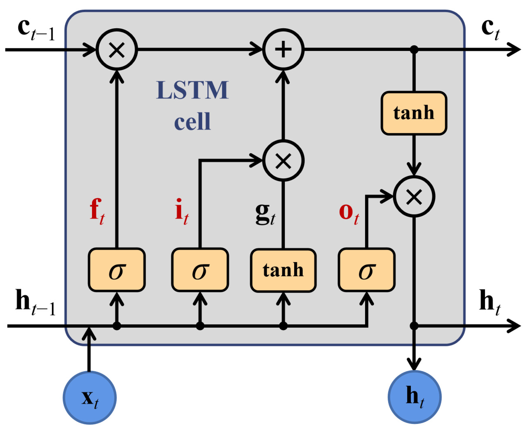
  37. Hochreiter, S.; Schmidhuber, J. Long short-term memory. Neural Comput. 1997, 9, 1735–1780. [Google Scholar] [CrossRef]
Figure 1. Schematic diagram of the multi-claw salvage system with SAHCs and strand jack lifters.
Jmse 11 00998 g001
Figure 2. Schematic diagram of the barge–shipwreck motion system, the salvage claws are omitted.
Jmse 11 00998 g002
Figure 3. Schematic diagram of an SAHC hydraulic system.
Jmse 11 00998 g003
Figure 4. Considered sea conditions in the hydrodynamic analysis for the salvage barge and their purposes.
Jmse 11 00998 g004
Figure 5. The heave and pitch RAOs of the salvage barge from the hydrodynamic analysis, the blue line denotes the heave RAO and the orange line denotes the pitch RAO.
Jmse 11 00998 g005
Figure 6. The testing sequences of the salvage barge from hydrodynamic analysis, during the sea condition of 3 m significant wave height and 12 s peak period.
Jmse 11 00998 g006
Figure 7. Inner structure of an LSTM cell at t time step.
Jmse 11 00998 g007
Figure 8. Structure diagram of the proposed LSTM-based motion predictive neural network, t denotes the current time step.
Jmse 11 00998 g008
Figure 9. The prediction RMSEs of different sequential input time sizes: (a) heave motion; (b) pitch motion.
Jmse 11 00998 g009
Figure 10. One-step prediction of the barge’s heave and pitch motions.
Jmse 11 00998 g010
Figure 11. Continuous rolling predictions of the barge’s heave and pitch motions during different predictive horizons.
Jmse 11 00998 g011
Figure 12. The lead–lag influence of the heave compensation to the shipwreck’s heave and pitch motions.
Jmse 11 00998 g012
Figure 13. Simulation results of the barge motions without measuring noise, including the compensation conditions of non-compensation, PHC mode, SAHC mode without motion prediction (original), and SAHC mode with motion prediction (pts denotes t seconds prediction).
Jmse 11 00998 g013
Figure 14. Noise pollution and filtering results of barge’s motion data.
Jmse 11 00998 g014
Figure 15. Simulation results of the barge motions with measuring noise, including the compensation conditions of non-compensation, SAHC mode without motion prediction (original), and SAHC mode with motion prediction (pts denotes t seconds prediction).
Jmse 11 00998 g015
Table 1. Parameters for barge hydrodynamic analysis.
Salvage BargeMooring System
Size (m)140 × 56 × 8.88Line typeCatenary stud chain
Pitch inertial (kg·m2)4.3 × 10¹⁰Mooring radius (km)2.4
Draft (m)3.6Chain length (m)2560
Displacement (t)26159Unit mass (kg/m)107
Mooring systemChain diameter (mm)70
Stiffness (kN/m)4.9 × 105Maximum expected tension (kN)4196
Pre-tension (kN)746.7
Table 2. Layer parameters of the LSTM-based predictive neural network, with the mini-batch size denoted by p.
Layer SequenceLayerTensor Size
1Sequential inputP × 2 × n
2LSTM layerP × n × 1024
3LSTM last outputP × 1024
4Fully connected layerP × 512
5Fully connected layerP × 512
6Output layerP × 2m
Table 3. Key parameters of the salvage system for numerical simulation.
ParameterUnitValueNotation
Shipwreck motion dynamicPitch inertialkg·m21.7 × 109Iw
Additional coefficient 1.5kadd
Lifting slingWire rope diametermm50
Wire rope number 8
600 m sling masst53.98ms
Sling stiffnesskN/m1.31 × 103ks
Passive part of SAHCCylinder total aream20.25Ap
Accumulator volumeL1500Vp
Adiabatic index 1.4n
Active part of SAHCSource pressureMPa20Ps
Cylinder total aream20.25Aa
Orifice flow coefficient 0.6Cd
Throttle gradientm0.0628ω
Oil densitykg/m3860ρoil
Oil bulk modulusMPa1000βe
SAHCPiston total masskg5000mc
Damping coefficientN/(m/s)1 × 104bc
Disclaimer/Publisher’s Note: The statements, opinions and data contained in all publications are solely those of the individual author(s) and contributor(s) and not of MDPI and/or the editor(s). MDPI and/or the editor(s) disclaim responsibility for any injury to people or property resulting from any ideas, methods, instructions or products referred to in the content.

