MPC-Based Collaborative Control of Sail and Rudder for Unmanned Sailboat

Abstract

In the traditional motion control method of an unmanned sailboat, the sail and rudder are divided into two independent controllers. The sail is used to obtain the thrust and the rudder is used to adjust the yaw angle. The traditional control method does not consider the synergy between the two controllers and ignores the influence of the roll angle on sailing. It is easy for these methods to cause an excessive roll angle and large yaw angle error, which will weaken the safe navigation and accurate path tracking of an unmanned sailboat. This paper presents a collaborative control method of sail and rudder based on model predictive control. A four-degree-of-freedom kinematics and dynamics model of the unmanned sailboat considering roll angle was established, with the yaw angle and roll angle as the control objectives at the same time. The collaborative control method outputs sail angle and rudder angle simultaneously. By comparing the motion of this method and the separation control of sail and rudder under the same wind field conditions, it is verified that the collaborative control has better effects of yaw angle control and roll angle limitation and can obtain a more accurate path tracking effect.

1. Introduction

Unlimited by carried fuel, an unmanned sailboat is powered by wind and solar energy and has the advantages of long-duration and wide-range cruising on the sea surface [1]. In recent years, unmanned sailboats have played a unique advantage in broad applications such as marine data collection, environmental monitoring, ocean observation, etc. [2]. In the traditional rudder control of an unmanned sailboat, the most common method is PID control. However, PID control is prone to steady-state error and oscillation in actual unmanned sailboat control. The sail control is usually the maximum thrust sail angle method, and the control goal is to maximize the speed. However, the maximum thrust sail angle method does not take into account the limitation of roll angle and lateral displacement, which will cause the excessive roll angle. Excessive roll angle will affect navigation safety and cause a poor path tracking effect in actual control.

In recent years, many domestic and foreign scholars have conducted a lot of research on the improvement of traditional motion control strategies. Dong et al. [3] proposed a Gaussian process model predictive control (GPMPC) method based on data-driven learning technology for rudder control, which improved the control effect of yaw angle. Jouffroy et al. [4] designed a nonlinear rudder controller using the integrator backstepping method and achieved a good heading control effect. Shen ZP et al. [5] proposed a rudder control strategy of the adaptive recursive sliding mode dynamic surface for unmanned sailboats’ course control. In addition, neural networks with memory and prediction functions have begun to enter the field of surface ship control [6]. Based on the kinematics model, Astrov [7] designed a seven-layer neural network predictive rudder controller to control the course of unmanned sailboats. In the later research, scholars gradually began to pay attention to the problem of sail control and put forward some methods of speed adjustment and roll angle limitation. Zhang et al. [8] proposed a robust fuzzy speed regulator by integrating dynamic surface control and robust fuzzy damping technology, which lost speed in exchange for a smaller roll angle. Corno et al. [9] proposed an optimized sail controller based on the improved extreme search method to keep unmanned sailboats at the best speed in a changing wind. Saoud et al. [10] proposed a method of sail angle control that maximizes speed based on limiting the roll angle, effectively limiting the roll angle in sailing. Deng et al. [11] designed an event-triggered composite adaptive fuzzy control law, which added the roll angle constraint method into the sail control law to prevent unmanned sailboats from capsizing.

The above methods all consider the control of rudder and sail separately and do not consider the synergy between the action of rudder and sail. In order to achieve the comprehensive best effect of the control of an unmanned sailboat, the sail and rudder cooperation provides a new way of thinking. Sun et al. [12] proposed a control strategy for wind-surfing navigation based on force polar coordinates. In this algorithm, the sail angle and rudder angle are output through the same control algorithm, and they cooperate with each other to obtain the maximum speed in the course of wind-surfing navigation. However, this collaborative control method is not used for yaw angle control and path tracking.

Collaborative sail and rudder control is required to solve multi-input multi-output control problems as well as to be capable of adapting to the complex nonlinear motion of an unmanned sailboat. MPC is suited to deal with complex nonlinear model problems, allowing one algorithm to simultaneously output rudder control signals and sail control signals. MPC is an optimization control algorithm firstly proposed by Richalet [13] in 1979. It uses the known model and current state quantity to predict the future output of the system and determines the current optimal control target value of the system through online time-domain rolling optimization and feedback correction methods. Gao et al. [14] combined MPC controllers with neural network adaptive controllers for positioning control and tracking optimization of underwater robots. Zhang et al. [15] established a kinematic dynamics model of AUV with six degrees of freedom and proposed a 3D underwater trajectory tracking method for AUV based on MPC.

Inspired by the above research, this paper proposes an MPC-based collaborative control method for the sail and rudder of an unmanned sailboat with the goal of simultaneously controlling the yaw angle and limiting the roll angle.

Based on the four-degree-of-freedom kinematics and dynamics model of the unmanned sailboat, this method converts the problem of yaw angle and roll angle control into an optimization problem with constraints. The constraints include input constraints and state constraints, and then the optimization problem is transformed into a standard convex quadratic programming problem that can be calculated online. When the unmanned sailboat reaches a new state, the optimal input of the next moment is recalculated according to the current state and expected state, and the rolling optimization is carried out according to this cycle. Finally, based on the mature MMG dynamics model and the four-degree-of-freedom kinematics model of the unmanned sailboat, the simulation study verifies the effectiveness of the control method. The innovative aspects of this paper can be summarized as:

(1) The tracking of yaw angle and the restriction of roll angle are considered in the control target. It is beneficial to reduce the error of path tracking and is more suitable for the actual motion control of ocean observation unmanned sailboats.

(2) Considering the role of roll angle in the motion control of the unmanned sailboat, the rudder and sail are combined to achieve the control goal by using the multi-input and multi-output characteristics of MPC.

This paper is divided into the following sections. The second section presents the kinematic dynamics model of the unmanned sailboat. The third section presents the MPC-based sail and rudder cooperative control strategy. Simulation results are given in the fourth section. The fifth section provides a summary and an outlook for future work.

2. Model

Most of the traditional motion control studies consider the motion of an unmanned sailboat as a three-degree-of-freedom planar motion, i.e., only surge, sway and yaw are considered. However, in the actual ocean navigation, an unmanned sailboat will be subjected to wind and waves, and it is more reasonable to describe it by a four-degree-of-freedom motion model including the roll angle.

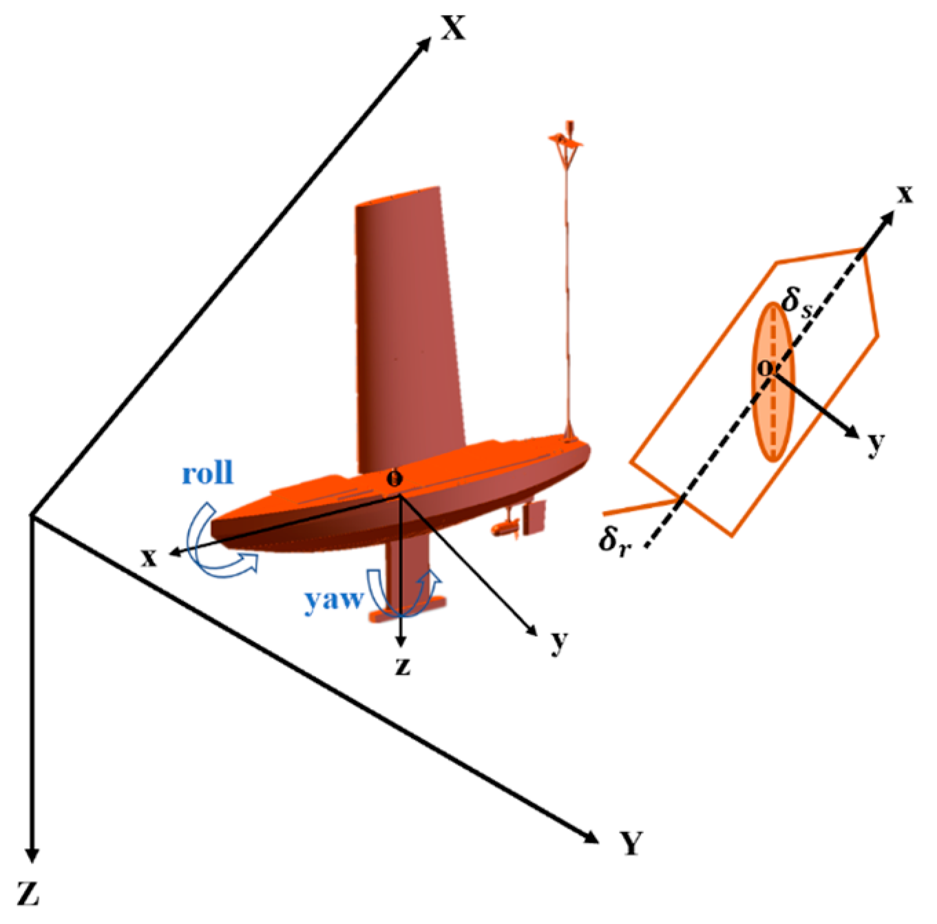
2.1. Reference Coordinate System

In order to clearly describe the four-degree-of-freedom motion of the unmanned sailboat, the inertial coordinate system (i-frame) O-XYZ and the appendage coordinate system (b-frame) o-xyz are defined as shown in Figure 1. O is the origin of the inertial coordinate system. OX points due east, OY points due north and OZ is perpendicular to the Earth’s surface and points down. The wind direction and boat direction in the inertial coordinate system are in the angular range [0°, 360°), with the OX positive direction as 0° and increasing clockwise. o is the origin of the appendage coordinate system. ox points to the bow, oy points to starboard and oz points to the bottom of the sailboat. The wind direction in the appendage coordinate system takes values in the interval [0°, 180°], 0° for perfectly upwind and 180° for perfectly downwind. The wind from the starboard side is positive and the wind from the port side is negative. Sail angle is defined as positive for sail to starboard and negative for sail to port. The rudder angle is defined as positive for rudder to starboard and negative for rudder to port.

2.2. Kinematic Model

In the inertial coordinate system, x denotes the displacement in the x-axis direction, y denotes the displacement in the y-axis direction and ψ denotes the yaw angle. ψ is 0° in the positive direction of the y-axis and increases clockwise, $0\le \psi <2\mathsf{\pi }$. ϕ denotes the roll angle, $-\frac{\pi }{2}\le \varphi \le \frac{\pi }{2}$. In the appendage coordinate system, u denotes the velocity in the x-axis direction, v denotes the velocity in the y-axis direction, r denotes the yaw angle angular velocity and p denotes the roll angular velocity.

In this paper, a four-degree-of-freedom kinematic model considering the roll angle is used:

$$\{\begin{array}{c}\dot{x}=u\cos \psi -v\cos \varphi \sin \psi \\ \dot{y}=u\sin \psi +v\cos \varphi \cos \psi \\ \dot{\psi }=r\cos \varphi \\ \dot{\varphi }=p\end{array}$$

(1)

where $\dot{x}$ denotes the velocity in the $x$-axis direction, $\dot{y}$ denotes the velocity in the $y$-axis direction, $\dot{\psi }$ denotes the angular velocity in the yaw angle direction and $\dot{\varphi }$ denotes the angular velocity in the roll angle direction.

The wind observed in the inertial coordinate system is the true wind. The true wind speed is defined as $V_{tw}$ and the true wind direction is defined as ${\alpha }_{tw}$. The wind observed in the appositional coordinate system is the apparent wind. The apparent wind speed is defined as $V_{aw}$ and the apparent wind direction is defined as ${\alpha }_{aw}$. V is the actual speed of the sailboat and satisfies $V^2=u^2+v^2$, where $\mathit{V}$, $V_{tw}$ and $V_{aw}$ satisfy the vector triangle. The sail angle ${\delta }_s$ is defined as the angle between the chord of the sail and the longitudinal axis of the sailboat. The angle of attack ${\alpha }_s$ is defined as the angle between the apparent wind and the chord of the sail, satisfying ${\alpha }_s={\alpha }_{aw}-{\delta }_s$, and the rudder angle is defined as ${\delta }_r$.

2.3. Dynamics Model

The dynamics model uses the MMG model proposed by the Ship Manoeuvring Mathematical Model Group of the Japan Towing Tank Committee (JTTC) [16]. The MMG model is a well-established model of sailboat dynamics built according to the physical sense. Its main feature is the decomposition of the hydrodynamic forces and moments acting on an unmanned sailboat into hydrostatic resistance, additional resistance on the hull, rudder force and sail force. In addition, the forces and moments coupled between them are also considered.

Based on the MMG model, the dynamics model of the unmanned sailboat in this paper can be expressed as:

$$\{\begin{array}{c}m\left(\dot{u}-v\dot{\psi }\right)=X_U+X_{hull}+X_{rudder}+X_{sail}\\ m\left(\dot{v}+u\dot{\psi }\right)=Y_{hull}+Y_{rudder}+Y_{sail}\\ \left(I_{xx}+J_{xx}\right)\ddot{\varphi }=K_{hull}+K_{rudder}+K_{sail}+K_{stability}\\ \left(I_{zz}+J_{zz}\right)\ddot{\psi }=N_{hull}+N_{rudder}+N_{sail}\end{array}$$

(2)

where $\ddot{\psi }$ denotes the angular acceleration of the yaw angle, $\ddot{\varphi }$ denotes the angular acceleration of the roll angle, $I_{xx}$ denotes the rotational inertia around the x-axis in the attachment coordinate system, $J_{xx}$ denotes the additional rotational inertia around the x-axis in the attachment coordinate system, $I_{zz}$ denotes the rotational inertia around the z-axis in the attachment coordinate system and $J_{zz}$ denotes the additional rotational inertia around the z-axis in the attachment coordinate system. $X_U$ denotes the residuary resistance of hull. $X_{hull}$, $Y_{hull}$, $K_{hull}$ and $N_{hull}$ denote the force and moment from additional hull resistance, and they can be expressed as

$$\{ \begin{array}{c}{X}_{hull}=\left(X_{VV}^{\prime }{V\prime }^2+X_{\phi \phi }^{\prime }{\varphi }^2+X_{VVVV}^{\prime }{V\prime }^4\right)\left(\frac{1}{2}\rho V_B^{2}LD\right)\\ Y_{hull}=\left(Y_V^{\prime }{V}^{\prime }+Y_{\phi }^{\prime }\varphi +Y_{V\phi \phi }^{\prime }{V}^{\prime }{\varphi }^2+Y_{VV\phi }^{\prime }{V\prime }^2\varphi +Y_{VVV}^{\prime }{V\prime }^3\right)\left(\frac{1}{2}\rho V_B^{2}LD\right)\\ K_{hull}=\left(K_V^{\prime }{V}^{\prime }+K_{\phi }^{\prime }\varphi +K_{V\phi \phi }^{\prime }{V}^{\prime }{\varphi }^2+K_{VV\phi }^{\prime }{V\prime }^2\varphi +K_{VVV}^{\prime }{V\prime }^3\right)\left(\frac{1}{2}\rho V_B^{2}L{D}^2\right)\\ N_{hull}=\left(N_V^{\prime }{V}^{\prime }+N_{\phi }^{\prime }\varphi +N_{V\phi \phi }^{\prime }{V}^{\prime }{\varphi }^2+N_{VV\phi }^{\prime }{V\prime }^2\varphi +N_{VVV}^{\prime }{V\prime }^3\right)\left(\frac{1}{2}\rho V_B^2{L}^{2}D\right)\end{array}$$

(3)

where $X_{VV}^{\prime }$, $X_{\phi \phi }^{\prime }$, $X_{VVVV}^{\prime }$, $Y_V^{\prime }$, $Y_{\phi }^{\prime }$, $Y_{V\phi \phi }^{\prime }$, $Y_{VV\phi }^{\prime }$, $Y_{VVV}^{\prime }$, $K_V^{\prime }$, $K_{\phi }^{\prime }$, $K_{V\phi \phi }^{\prime }$, $K_{VV\phi }^{\prime }$, $K_{VVV}^{\prime }$, $N_V^{\prime }$, $N_{\phi }^{\prime }$, $N_{V\phi \phi }^{\prime }$, $N_{VV\phi }^{\prime }$ and $N_{VVV}^{\prime }$ denote the hydrodynamic coefficient of additional hull resistance. $V^{\prime }$ denotes the sine function of the drift angle. $V^{\prime }=\sin \beta$, and $\beta$ denotes drift angle. $V_B$ denotes the speed of the sailboat, and $V_B=\sqrt{u^2+v^2}$. $L$ denotes the length of the sailboat. $D$ denotes the draft of the sailboat.

$X_{rudder}$, $Y_{rudder}$, $K_{rudder}$ and $N_{rudder}$ denote the force and moment on the rudder, and they can be expressed as

$$\{\begin{array}{c}{X}_{rudder}=C_{X\delta }\sin {\alpha }_R\sin {\delta }_r\left(\frac{1}{2}\rho V_B^{2}LD\right)\\ Y_{rudder}=C_{Y\delta }\sin {\alpha }_R\cos {\delta }_r\cos \varphi \left(\frac{1}{2}\rho V_B^{2}LD\right)\\ K_{rudder}=C_{K\delta }\sin {\alpha }_R\cos {\delta }_r\left(\frac{1}{2}\rho V_B^{2}L{D}^2\right)\\ N_{rudder}=C_{N\delta }\sin {\alpha }_R\cos {\delta }_r\cos \varphi \left(\frac{1}{2}\rho V_B^2{L}^{2}D\right)\end{array}$$

(4)

where $C_{X\delta }$, $C_{Y\delta }$, $C_{K\delta }$ and $C_{N\delta }$ denote the rudder force coefficient. $\delta$ denotes rudder angle. ${\alpha }_R$ denotes the angle of attack of the rudder, and ${\alpha }_R=\delta +\beta$. $K_{stability}$ denotes the restoring moment of initial stability, and it can be expressed as

$$K_{stability}=-mg\overline{GM}\sin \varphi$$

(5)

where $m$ denotes the mass of the sailboat, $g$ denotes gravitational acceleration and $\overline{GM}$ denotes initial stability height. Among them, this paper focuses on the forces and moments acting on the sail, with particular attention to the roll moments of the sail. $X_{sail}$, $Y_{sail}$, $K_{sail}$ and $N_{sail}$ denote the forces and moments on the sail, and they can be expressed as

$$\{\begin{array}{c}{X}_{sail}=C_x{\cos }^2\varphi \frac{1}{2}{\rho }_a{V}_{aw}^2{S}_A\\ Y_{sail}=C_y{\cos }^2\varphi \frac{1}{2}{\rho }_a{V}_{aw}^2{S}_A\\ K_{sail}=-C_y\left(\frac{z_{GCE}^G}{\sqrt{S_A}}\right)\cos \varphi \frac{1}{2}{\rho }_a{V}_{aw}^2{S}_A^{\frac{3}{2}}\\ N_{sail}=\{C_y\left(\frac{x_{GCE}^G}{\sqrt{S_A}}\right)+C_x\left(\frac{z_{GCE}^G}{\sqrt{S_A}}\right)\sin \varphi \}{\cos }^2\varphi \frac{1}{2}{\rho }_a{V}_{aw}^2{S}_A^{\frac{3}{2}}\end{array}$$

(6)

where $C_x$ denotes the sail longitudinal thrust coefficient, $C_y$ denotes the sail transverse thrust coefficient, ${\rho }_a$ denotes the density of air and $S_A$ denotes the wind area of the sail. $x_{GCE}^G$ and $z_{GCE}^G$ denote the coordinates of the sail force point relative to the center of gravity.

The longitudinal and lateral thrust coefficients of the sail are determined by the dynamic coefficient, drag coefficient and relative wind angle of the sail itself. The dynamic coefficient and drag coefficient of the sail are obtained from the sail test. They can be expressed as

$$\{\begin{array}{c}{C}_x=C_l\sin \left({\alpha }_{aw}\right)-C_d\cos \left({\alpha }_{aw}\right)\\ C_y=C_l\cos \left({\alpha }_{aw}\right)+C_d\sin \left({\alpha }_{aw}\right)\end{array},$$

(7)

where $C_l$ denotes the power coefficient of the sail and $C_d$ denotes the drag coefficient of the sail.

3. Collaborative Control Strategy

MPC is a control strategy based on numerical optimization, which designs a system model to predict future control inputs and future state responses. MPC has a good theoretical basis. It optimizes the state response of the system at each cycle interval by calculating the sequence of future system input adjustments. By minimizing the cost function, the optimal control input sequence for the next N sampling interval is obtained. When solving optimization problems, input constraints and state constraints can be explicitly dealt with to improve the robustness of the system. The main characteristics of MPC are rolling optimization and feedback correction, which can effectively reduce the error in the closed-loop system. Therefore, the MPC control system can achieve good stability, optimality and robustness.

The unmanned sailboat kinematic model (1) and dynamics model (2) correspond to eight nonlinear functions, denoted as $f_1$,$f_2$,$f_3$,$f_4$,$f_5$,$f_6$,$f_7$,$f_8$. We define the state quantities as $\mathit{x}={\left[x y \psi \varphi u v r p\right]}^T$ in the inertial coordinate system. We define the control quantities as $\mathit{u}={\left[{\delta }_s {\delta }_r\right]}^T$ in the appendage coordinate system. The nonlinear equation of the kinematic and dynamics model can be written as:

$$\dot{x}=f\left(\mathit{x},\mathit{u}\right)$$

(8)

In this paper, the state quantities we want to control are the yaw angle $\psi$ and the roll angle $\varphi$, so we define the output quantities as $\mathit{y}={\left[\psi \varphi \right]}^T$, satisfying $\mathit{y}=C\mathit{x}$, where $C=\left[O_{2*2} I_2 O_{2*4}\right]$. We assume that the desired yaw angle ${\psi }_d$ and the desired roll angle ${\varphi }_d$ are known in advance. The desired output quantities can be expressed as ${\mathit{y}}_d={\left[{\psi }_d {\varphi }_d\right]}^T$. Let the target state quantities be ${\mathit{x}}_d={\left[x_d y_d {\psi }_d {\varphi }_d u_d v_d r_d p_d\right]}^T$. From $\mathit{y}=C\mathit{x}$, we can deduce that ${\mathit{y}}_d=C{\mathit{x}}_d$. From ${\mathit{y}}_d=C{\mathit{x}}_d$, we can deduce that the target state quantities are ${\mathit{x}}_{\mathit{d}}=C^{+}{\mathit{y}}_{\mathit{d}}$, and $C^{+}$ is the pseudo-inverse matrix of $C$. From $\tilde{y}=\mathit{y}-{\mathit{y}}_{\mathit{d}}$, which represents the increment of the output quantities, then we obtain the increment of state quantities: $\tilde{\mathit{x}}=\mathit{x}-{\mathit{x}}_d$. The desired sail angle ${\delta }_{sd}$ and the desired rudder angle ${\delta }_{rd}$ can be calculated from the desired yaw angle, roll angle and real-time motion state. We define the desired control quantities as ${\mathit{u}}_d={\left[{\delta }_{sd} {\delta }_{rd}\right]}^T$, and define the quantities vector increment as $\tilde{\mathit{u}}=\mathit{u}-{\mathit{u}}_d$.

The controller design is divided into the following steps: prediction, constraint conditions, optimization and rolling time domain optimization.

3.1. Prediction

This part is the key step of model predictive control. Through the kinematics and dynamics model of the unmanned sailing boat and the current state quantity, the output quantity for the limited time in the future can be predicted.

The inputs of this part are target yaw ${\psi }_d$, target roll ${\varphi }_d$ and apparent wind angle ${\alpha }_{aw}$. Through the target yaw ${\psi }_d$ and apparent wind angle ${\alpha }_{aw}$, the optimal sail angle strategy can calculate the desired sail angle ${\delta }_{sd}$. The desired rudder angle ${\delta }_{rd}$ is usually set to 0. From ${\mathit{u}}_d={\left[{\delta }_{sd} {\delta }_{rd}\right]}^T$, we can calculate ${\mathit{u}}_d$. From ${\mathit{y}}_d={\left[{\psi }_d {\varphi }_d\right]}^T$, we can calculate ${\mathit{y}}_d$. From ${\mathit{x}}_d=C^{+}{\mathit{y}}_d$, we can calculate ${\mathit{x}}_d$. According to the sailboat state vector $\mathit{x}$ and control vector $\mathit{u}$ measured by the sensor, $\tilde{\mathit{x}}$ and $\tilde{\mathit{u}}$ can be calculated.

A Taylor expansion of Equation (8) at the point $\left({\mathit{x}}_d,{\mathit{u}}_d\right)$, keeping only the first-order terms and ignoring the higher-order terms, yields

$$\dot{\mathit{x}}=f\left({\mathit{x}}_d,{\mathit{u}}_d\right)+\frac{\partial f}{\partial \mathit{x}}{|}_{\mathit{u}={\mathit{u}}_d}^{\mathit{x}={\mathit{x}}_d}\left(\mathit{x}-{\mathit{x}}_d\right)+\frac{\partial f}{\partial \mathit{u}}{|}_{\mathit{u}={\mathit{u}}_d}^{\mathit{x}={\mathit{x}}_d}\left(\mathit{u}-{\mathit{u}}_d\right)$$

(9)

where $A_J=\frac{\partial f}{\partial x}{|}_{\mathit{u}={\mathit{u}}_d}^{\mathit{x}={\mathit{x}}_d}$ is the Jacobi matrix for which $f\left({\mathit{x}}_d,{\mathit{u}}_d\right)$ is biased against ${\mathit{x}}_d$. $B_J=\frac{\partial f}{\partial u}{|}_{\mathit{u}={\mathit{u}}_d}^{\mathit{x}={\mathit{x}}_d}$ is the Jacobi matrix of $f\left({\mathit{x}}_d,{\mathit{u}}_d\right)$ for the bias derivative of ${\mathit{u}}_d$.

According to the equation satisfying ${\dot{\mathit{x}}}_d=f\left({\mathit{x}}_d,{\mathit{u}}_d\right)$, $\dot{\tilde{\mathit{x}}}=\dot{\mathit{x}}-{\dot{\mathit{x}}}_d$. The derivative of the increment of the state quantity is obtained: $\dot{\tilde{\mathit{x}}}=A_J\tilde{\mathit{x}}+B_J\tilde{\mathit{u}}$. The forward Euler method can be expressed as a discrete form with a sampling period of T, namely $\dot{\tilde{\mathit{x}}}=\frac{\tilde{x}\left(k+1\right)-\tilde{\mathit{x}}\left(k\right)}{T}$, yielding $\tilde{\mathit{x}}\left(k+1\right)=\left(T{A}_J\left(k\right)+E\right)\tilde{\mathit{x}}\left(k\right)+T{B}_J\left(k\right)\tilde{\mathit{u}}\left(k\right)$, denoted as

$$\tilde{\mathit{x}}\left(k+1\right)=A\left(k\right)\tilde{\mathit{x}}\left(k\right)+B\left(k\right)\tilde{\mathit{u}}\left(k\right)$$

(10)

where $A\left(k\right)=T{A}_J\left(k\right)+E,B\left(k\right)=T{B}_J\left(k\right).$

We generate the prediction matrix for the state volume increments:

$$\{\begin{array}{c}\tilde{\mathit{x}}\left(k+1\right)=A\tilde{\mathit{x}}\left(k\right)+B\tilde{\mathit{u}}\left(k\right)\\ \tilde{\mathit{x}}\left(k+2\right)=A^2\tilde{\mathit{x}}\left(k\right)+AB\tilde{\mathit{u}}\left(k\right)+B\tilde{\mathit{u}}\left(k+1\right)\\ \tilde{\mathit{x}}\left(k+3\right)=A^3\tilde{\mathit{x}}\left(k\right)+A^{2}B\tilde{\mathit{u}}\left(k\right)+AB\tilde{\mathit{u}}\left(k+1\right)+B\tilde{\mathit{u}}\left(k+2\right)\\ ⋮\\ \tilde{\mathit{x}}\left(k+N\right)=A^N\tilde{\mathit{x}}\left(k\right)+A^{N-1}B\tilde{\mathit{u}}\left(k\right)+A^{N-2}B\tilde{\mathit{u}}\left(k+1\right)+\cdots +B\tilde{\mathit{u}}\left(k+N-1\right)\end{array}$$

(11)

Simplified as

$$\tilde{X}\left(k\right)=\overline{A}\left(k\right)\tilde{\mathit{x}}\left(k\right)+\overline{B}\left(k\right)\tilde{U}\left(k\right)$$

(12)

where $\tilde{X}\left(k\right)=\left[\begin{array}{c}\tilde{\mathit{x}}\left(k+1|k\right)\\ \tilde{\mathit{x}}\left(k+2|k\right)\\ ⋮\\ \tilde{\mathit{x}}\left(k+N|k\right)\end{array}\right]$,$\overline{A}\left(k\right)={\left[\begin{array}{cccc}A\left(k\right)& A{\left(k\right)}^2& \dots & A{\left(k\right)}^N\end{array}\right]}^T$, $\overline{B}\left(k\right)=\left[\begin{array}{cccc}B\left(k\right)& 0& \dots & 0\\ A\left(k\right)B\left(k\right)& B\left(k\right)& \cdots & 0\\ ⋮& ⋮& \ddots & ⋮\\ A{\left(k\right)}^{N-1}B\left(k\right)& A{\left(k\right)}^{N-2}B\left(k\right)& \cdots & B\left(k\right)\end{array}\right],\tilde{U}\left(k\right)=\left[\begin{array}{c}\tilde{u}\left(k|k\right)\\ \tilde{u}\left(k+1|k\right)\\ ⋮\\ \tilde{u}\left(k+N-1|k\right)\end{array}\right]$.

We define the predicted output vector as $\tilde{Y}\left(k\right)=\left[\begin{array}{c}\tilde{\mathit{y}}\left(k+1|k\right)\\ \tilde{\mathit{y}}\left(k+2|k\right)\\ ⋮\\ \tilde{\mathit{y}}\left(k+N|k\right)\end{array}\right]$, simplified as $\tilde{Y}\left(k\right)=\overline{C}\tilde{X}\left(k\right)$, where $\overline{C}=\left[\begin{array}{cccc}C{E}_{8*8}^1& O_{2*8}& \cdots & O_{2*8}\\ O_{2*8}& C{E}_{8*8}^2& \dots & O_{2*8}\\ ⋮& ⋮& \ddots & ⋮\\ O_{2*8}& O_{2*8}& \dots & C{E}_{8*8}^N\end{array}\right]$.

3.2. Constraint Conditions

In actual unmanned sailboat sailing, both the sail controller and rudder controller have their own action limits, i.e., upper limit $u_{max}$ and lower limit $u_{min}$. The range of the sail angle can be adjusted 0~90°, so the lower limit of the sail angle is 0 and the upper limit is 90°. The limit of both left and right rudder angle actions is 35°, so the lower limit is −35° for the left full rudder and the upper limit is 35° for the right full rudder. The upper limit vector is $u_{max}=\left[\begin{array}{c}{90}^{°}\\ {35}^{°}\end{array}\right]$ and the upper limit vector is $u_{min}=\left[\begin{array}{c}{0}^{°}\\ -{35}^{°}\end{array}\right]$.

We define the predictive control vector $U\left(k\right)$, and $U\left(k\right)$ satisfies the following $U_{min}\le U\left(k\right)\le U_{max}$, where $U_{min}=\left[\begin{array}{c}{E}_{2*2}^1{u}_{min}\\ E_{2*2}^2{u}_{min}\\ ⋮\\ E_{2*2}^N{u}_{min}\end{array}\right]$ and $U_{max}=\left[\begin{array}{c}{E}_{2*2}^1{u}_{max}\\ E_{2*2}^2{u}_{max}\\ ⋮\\ E_{2*2}^N{u}_{max}\end{array}\right]$. We define the control vector increment $\tilde{U}\left(k\right)$, with $\tilde{U}\left(k\right)$ satisfying $U_{min}-U_d\left(k\right)\le \tilde{U}\left(k\right)\le U_{max}-U_d\left(k\right)$, where $U_d\left(\mathrm{k}\right)=\left[\begin{array}{c}{u}_d\left(k|k\right)\\ u_d\left(k+1|k\right)\\ ⋮\\ u_d\left(k+N-1|k\right)\end{array}\right]$. The transformation is $\{\begin{array}{c}\tilde{U}\left(k\right)\le U_{max}-U_d\left(k\right)\\ -\tilde{U}\left(k\right)\le -U_{min}+U_d\left(k\right)\end{array}$, abbreviated as $L\tilde{U}\left(k\right)\le l\left(k\right),$ where $L=\left[\begin{array}{c}{I}_{2N}\\ -I_{2N}\end{array}\right],l\left(k\right)=\left[\begin{array}{c}{U}_{max}-U_d\left(k\right)\\ -U_{min}+U_d\left(k\right)\end{array}\right].$

3.3. Optimization

The inputs of this part are the state quantity prediction matrix $\tilde{X}\left(k\right)$ and control quantity prediction matrix $\tilde{U}\left(k\right)$, $\overline{A}\left(k\right)$, $\overline{B}\left(k\right)$ and $l\left(k\right)$. The cost function of MPC-based sail and rudder collaborative control contains the output quantity deviation and the control quantity deviation, which are defined as follows:

$$\begin{array}{c}J={{\displaystyle \int }}_0^T[\Vert \mathit{y}\left(t\right)-{\mathit{y}}_d{\left(t\right)\Vert }_{Q_y}^2+\Vert \mathit{u}{\left(t\right)\Vert }_{Q_u}^2]dt\\ s.t L\tilde{U}\left(k\right)\le l\left(k\right)\end{array}$$

(13)

where $Q_y$ denotes the weight of the output quantity in the cost function and $Q_u$ denotes the weight of the control quantity in the cost function. Since $\mathit{y}=C\mathit{x}$ and $\mathit{x}=C^{+}\mathit{y}$, $C^{+}$ is the pseudoinverse matrix of $C$. From $Q_x=C^T{Q}_{y}C=C^{+}{Q}_{y}C$, we can derive $J\left(k\right)=\Vert \tilde{Y}{\left(k\right)\Vert }_{{\overline{Q}}_y}^2+\Vert \tilde{U}{\left(k\right)\Vert }_{{\overline{Q}}_u}^2=\Vert \tilde{X}{\left(k\right)\Vert }_{{\overline{Q}}_x}^2+\Vert \tilde{U}{\left(k\right)\Vert }_{{\overline{Q}}_u}^2$. By expanding the formula, we can have

$$J\left(k\right)=\Vert \overline{A}\left(k\right)\tilde{x}\left(k\right)+\overline{B}\left(k\right)\tilde{U}{\left(k\right)\Vert }_{{\overline{Q}}_x}^2+\Vert \tilde{U}{\left(k\right)\Vert }_{{\overline{Q}}_u}^2$$

(14)

where ${\overline{Q}}_x=\left[\begin{array}{cccc}{Q}_x& 0& \cdots & 0\\ 0& Q_x& \dots & 0\\ ⋮& ⋮& \ddots & ⋮\\ 0& 0& \dots & Q_x\end{array}\right] \mathrm{and} {\overline{Q}}_u=\left[\begin{array}{cccc}{Q}_u& 0& \cdots & 0\\ 0& Q_u& \dots & 0\\ ⋮& ⋮& \ddots & ⋮\\ 0& 0& \dots & Q_u\end{array}\right]$ can be simplified as:

$$\begin{array}{c}{\tilde{U}}^{*}\left(k\right)={}_{U\left(k\right)}{}^{arg min} \frac{1}{2}{\tilde{U}}^T\left(k\right)H\left(k\right)\tilde{U}\left(k\right)+f^T\left(k\right)\tilde{U}\left(k\right)\\ s.t L\tilde{U}\left(k\right)\le l\left(k\right)\end{array}$$

(15)

where $H\left(k\right)=2\left({\overline{B}}^T\left(k\right){\overline{Q}}_x\overline{B}\left(k\right)+{\overline{Q}}_u\right)$ and $f\left(k\right)=2{\overline{B}}^T\left(k\right){\overline{Q}}_x\overline{A}\left(k\right)$.

3.4. Rolling Time Domain Optimization

Since there are inevitable errors in the system modeling and errors in the first-order Taylor expansion of the system equations, the MPC control algorithm selects only the first set of control vectors ${\tilde{\mathit{u}}}^{*}\left(k\right)$ at a time for output. The ${\tilde{\mathit{u}}}^{*}\left(k\right)$ selects the first and second elements of ${\tilde{U}}^{*}\left(k\right)$, where ${\tilde{\mathit{u}}}^{*}\left(k\right)=\left[\begin{array}{c}{\tilde{U}}^{*}\left(k\right)\left[1\right]\\ {\tilde{U}}^{*}\left(k\right)\left[2\right]\end{array}\right]$. Waiting until the next time step and then recalculating the new control vector based on the feedback state quantity combined with the target state quantity to form a rolling time-domain optimization is as follows:

$${\mathit{u}}^{*}\left(k\right)=\mathit{u}\left(0\right)+{\tilde{\mathit{u}}}^{*}\left(k\right)$$

(16)

where ${\mathit{u}}^{*}\left(k\right)=\left[\begin{array}{c}{\delta }_s^{*}\left(k\right)\\ {\delta }_r^{*}\left(k\right)\end{array}\right]$.

The control law of sail angle:

$${\delta }_s^{*}\left(k\right)={\mathit{u}}^{*}\left(k\right)\left[1\right]$$

(17)

The control law of rudder angle:

$${\delta }_r^{*}\left(k\right)={\mathit{u}}^{*}\left(k\right)\left[2\right]$$

(18)

3.5. Controller Design Diagram

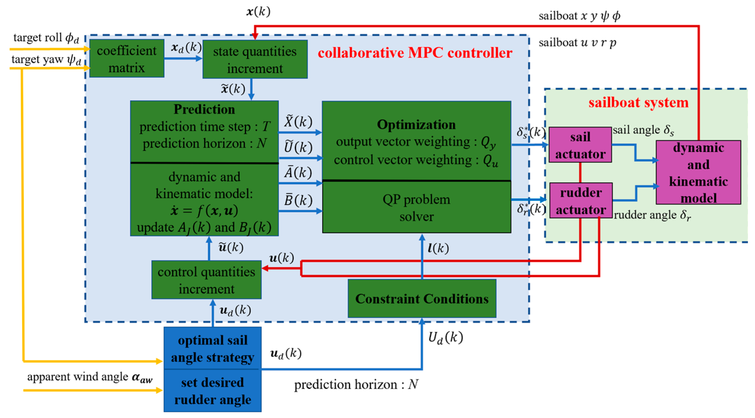
The controller design process for collaborative MPC control of the sail and rudder of the unmanned sailboat is shown in Figure 2.

The controller design process for collaborative MPC control of the sail and rudder of the unmanned sailboat is shown in Figure 2. The yellow arrow represents the external input quantity, the blue arrow represents the process quantity and the red arrow represents the feedback quantity. The core part of the controller includes prediction, constraint conditions and optimization. The prediction part reads the state quantities increment $\tilde{\mathit{x}}\left(k\right)$ and the control quantities increment $\tilde{\mathit{u}}\left(k\right)$, and calculates the prediction matrices $\tilde{X}\left(k\right)$, $\tilde{U}\left(k\right)$, $\overline{A}\left(k\right)$ and $\overline{B}\left(k\right)$ based on the known dynamics model and kinematics model of the unmanned sailboat. Based on the known upper and lower limits of sail angle and rudder angle, combined with the desired control matrix $U_d\left(\mathit{k}\right)$, the constraint conditions part calculates $l\left(\mathit{k}\right)$. The optimization part reads the prediction matrices and constraint conditions and converts them into a standard convex quadratic programming problem. By solving the quadratic programming problem, the optimization part calculates the optimal control quantities increment ${\tilde{U}}^{*}\left(k\right)$. The controller selects the first set of values as the output sail angle ${\delta }_s^{*}\left(k\right)$ and rudder angle ${\delta }_r^{*}\left(k\right)$. At the end of a time step, the calculation is repeated through feedback to achieve rolling optimization.

3.6. Algorithm

The Algorithm 1 in the following table is the process of collaborative MPC control of the sail and rudder of the unmanned sailboat.

Algorithm 1: MPC sail rudder collaborative control

Input: ${\mathit{y}}_d$ (desired output), $\mathit{u}\left(0\right)$ (initial control vector), T (prediction time step), N (prediction horizon), C(coefficient matrix), $Q_u$ (control vector weighting matric), $Q_y$ (output vector weighting matric), $u_{min}$, $u_{max}$ (control vector constraints) 1: k←1 2: x(k)← x(0) 3:compute $Q_x,{\overline{Q}}_x, {\overline{Q}}_u,U_{min},U_{max} ,\overline{C}$ 4:while k ≥ 0 do 5:    compute ${\mathit{u}}_d\left(k\right),{\mathit{x}}_d\left(k\right),\tilde{\mathit{u}}\left(k\right),\tilde{\mathit{x}}\left(k\right),A\left(k\right),B\left(k\right)$ 6:    update $\tilde{X}\left(k\right)$,$\tilde{U}\left(k\right),\overline{A}\left(k\right)$,$\overline{B}\left(k\right)$,$l\left(k\right)$ 7:    solve the QP problem 8:    get the first control vector ${\tilde{\mathit{u}}}^{*}\left(k\right)$ from ${\tilde{U}}^{*}\left(k\right)$ 9:    implement ${\delta }_s^{*}\left(k\right)$ and ${\delta }_r^{*}\left(k\right)$ to the sail and rudder 10: k← k + 1 11: measure the current $\mathit{x}\left(k\right)$ and $\mathit{u}\left(k\right)$ 12:end while

4. Simulation Results

In this section, the MPC-based sail and rudder collaborative control method of the unmanned sailboat is verified by simulation. The simulations were conducted on a desktop computer equipped with an AMD Ryzen5 3.6 GHz processor, using a simulator developed on the Simulink platform based on Matlab R2021a. The first simulation compares the control effect of MPC-based sail and rudder collaborative control with MPC-based separation control during sidewind sailing. The second simulation compares the sailing effect of the above two methods in a four-point sailing simulation experiment in a constant wind field.

The hydrodynamic and aerodynamic parameters of the unmanned sailboat used in the simulation are derived from the Fujin-class unmanned sailboat in the paper [17]. The specific parameters involved are shown in

Table 1. Fujin-class unmanned sailboat parameters.

Parameters	Value	Parameters	Value
L	8.80 m	$Y_{V\phi \phi }^{\prime }$	7.37 × 10−1
B	2.64 m	$Y_{VV\phi }^{\prime }$	−5.53 × 10−1
D	2.02 m	$Y_{VVV}^{\prime }$	3.07
$m$	4410 kg	$K_V^{\prime }$	2.80 × 10−1
$\overline{GM}$	1.45 m	$K_{\phi }^{\prime }$	3.36 × 10−3
$x_{CG}$	−0.60 m	$K_{V\phi \phi }^{\prime }$	−4.07 × 10−1
$I_R$	4.40 m	$K_{VV\phi }^{\prime }$	2.24 × 10−1
$S_a$	59.3 m2	$K_{VVV}^{\prime }$	−1.38
$m_x$	160 kg	$N_V^{\prime }$	−3.23 × 10−2
$m_y$	2410 kg	$N_{\phi }^{\prime }$	−1.52 × 10−2
$m_z$	12,000 kg	$N_{V\phi \phi }^{\prime }$	2.71 × 10−4
$I_{xx}$	17,700 kg·m2	$N_{VV\phi }^{\prime }$	−9.06 × 10−2
$I_{yy}$	33,100 kg·m2	$N_{VVV}^{\prime }$	−2.98 × 10−2
$I_{zz}$	17,200 kg·m2	$C_{X\delta }$	−3.79 × 10−2
$J_{xx}$	15,300 kg·m2	$C_{Y\delta }$	−1.80 × 10−1
$J_{yy}$	42,400 kg·m2	$C_{K\delta }$	9.76 × 10−2
$J_{zz}$	6700 kg·m2	$C_{N\delta }$	9.74 × 10−2
$X_{VV}^{\prime }$	3.38 × 10−1	${\rho }_a$	1.205 kg/m3
$X_{\phi \phi }^{\prime }$	1.40 × 10−3	${\rho }_w$	1025 kg/m3
$X_{VVVV}^{\prime }$	−1.84	$x_{GCE}^G$	0.67 m
$Y_V^{\prime }$	−5.35 × 10−1	$z_{GCE}^G$	−6.13 m
$Y_{\phi }^{\prime }$	−5.89 × 10−3	$S_w$	21 m2

.

Each basic parameter of the MPC algorithm is as follows: sampling time T = 0.5 s, number of prediction steps n = 10, output weight matrix $Q_y=diag\left(q_{\psi },q_{\varphi }\right)$ and control weight matrix $Q_u=diag\left(q_s,q_r\right)$. According to the MPC parameter selection method, a set of weight coefficients with a better control effect is selected among multiple reasonable sets of weights. The output weight matrix $Q_y=diag\left(1,2\right)$ and the control weight matrix $Q_u=diag\left(0.1,1\right)$ are selected for the sail and rudder collaborative control. Since the variation range of the yaw angle is $0~{360}^{°}$ and the variation range of the roll angle is $-{90}^{°}~{90}^{°}$, the yaw angle weight: roll angle weight = 1:2. The variation range of the sail angle is $0^{°}~{90}^{°}$, and the variation range of the rudder angle is $-{35}^{°}~{35}^{°}$. 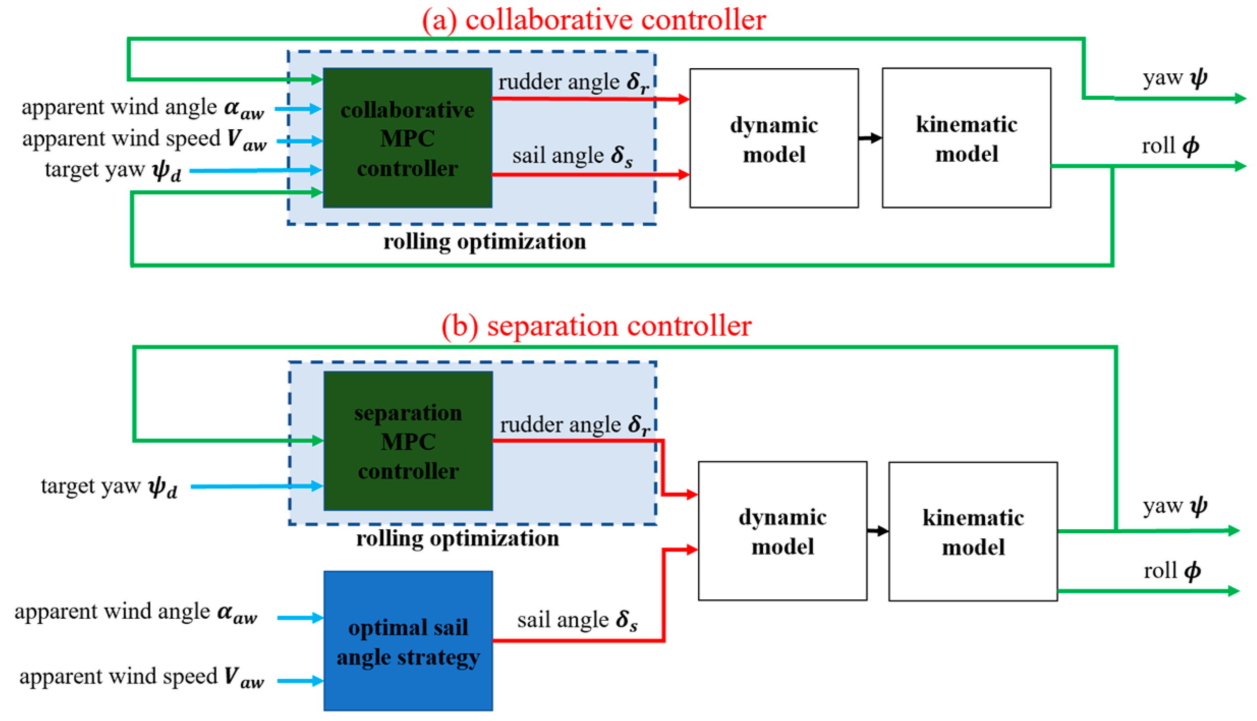The control weight of the sail angle should be reduced appropriately since the sail angle should take the optimal thrust sail angle as a reference. Set sail control weight: rudder control weight = 0.1:1. The flow and parameters of the MPC control algorithm used for separating the control rudder angle are the same as those of collaborative control, but the roll angle part is discarded in the model. The separated control output vector only contains the yaw angle, and the control weight is set as $Q_y=\left[1\right], Q_u=diag\left(0.1,1\right)$. The sail angle of the separation control adopts the traditional maximum thrust method, which means that the sail angle of the optimal thrust is selected according to the relative wind angle. The simulation flow of the two control methods is shown in Figure 3.

4.1. Comparison of Sail–Rudder Collaborative and Separation Control

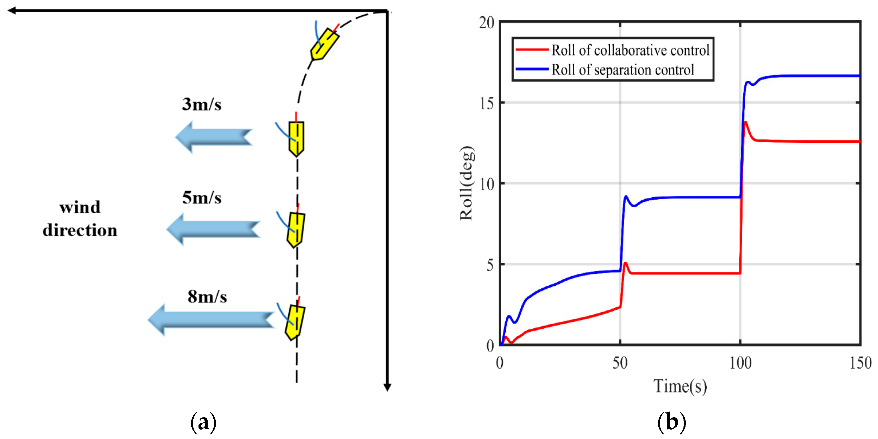
The challenge of unmanned sailboat control comes from sidewind sailing, because the roll angle of an unmanned sailboat is the largest when sailing in side wind. When sailing in side wind, the sail lateral force and roll moment are also larger, so the yaw angle control is challenged to some extent. Therefore, a comparison experiment between collaborative control and separation control is carried out for 90° positive sidewind sailing to better visualize the difference between the two control algorithms. The schematic diagram is shown in Figure 4a. The initial yaw angle $\psi$ is set to 180°, the initial roll angle $\varphi$ is 0°, the initial longitudinal speed $u$ is 2 m/s and the desired yaw angle ${\psi }_d$ is set to 90°. The wind direction is constant as ${\alpha }_{tw}={180}^{°}$, and the wind speed is gradually increasing:

$$V_{tw}=\{\begin{array}{c}3 \mathrm{m}/\mathrm{s},t\in \left[0,50s\right)\\ 5 \mathrm{m}/\mathrm{s},t\in \left[50,100s\right)\\ 8 \mathrm{m}/s,t\in \left[100,150s\right)\end{array}$$

The comparison of the roll angle of the sidewind sailing experiments is shown in Figure 4b.

From

Table 2. Roll angle of the collaborative control and separation control.

Roll	Collaborative Control (deg)	Separation Control (deg)
3 m/s	2.32	4.57
5 m/s	4.43	9.13
8 m/s	12.58	16.65

below, we can see that the roll angle of the collaborative control is smaller than that of the separation control under different wind speeds. In the 90° sidewind sailing, the collaborative control achieves better roll angle control compared with the separation control.

Since it is difficult to achieve no error in the yaw angle for positive sidewind navigation, the steady-state error of the yaw angle is adopted as the evaluation index. The smaller the steady-state error is, the better the control effect is. From $\psi ={{\displaystyle \int }}^{ }rdt\cos \varphi$, it can be seen that the yaw turning angle generated by the rudder is ${{\displaystyle \int }}^{ }rdt$. The larger the roll angle $\varphi$ is, the larger the yaw angle $\psi$ error is. 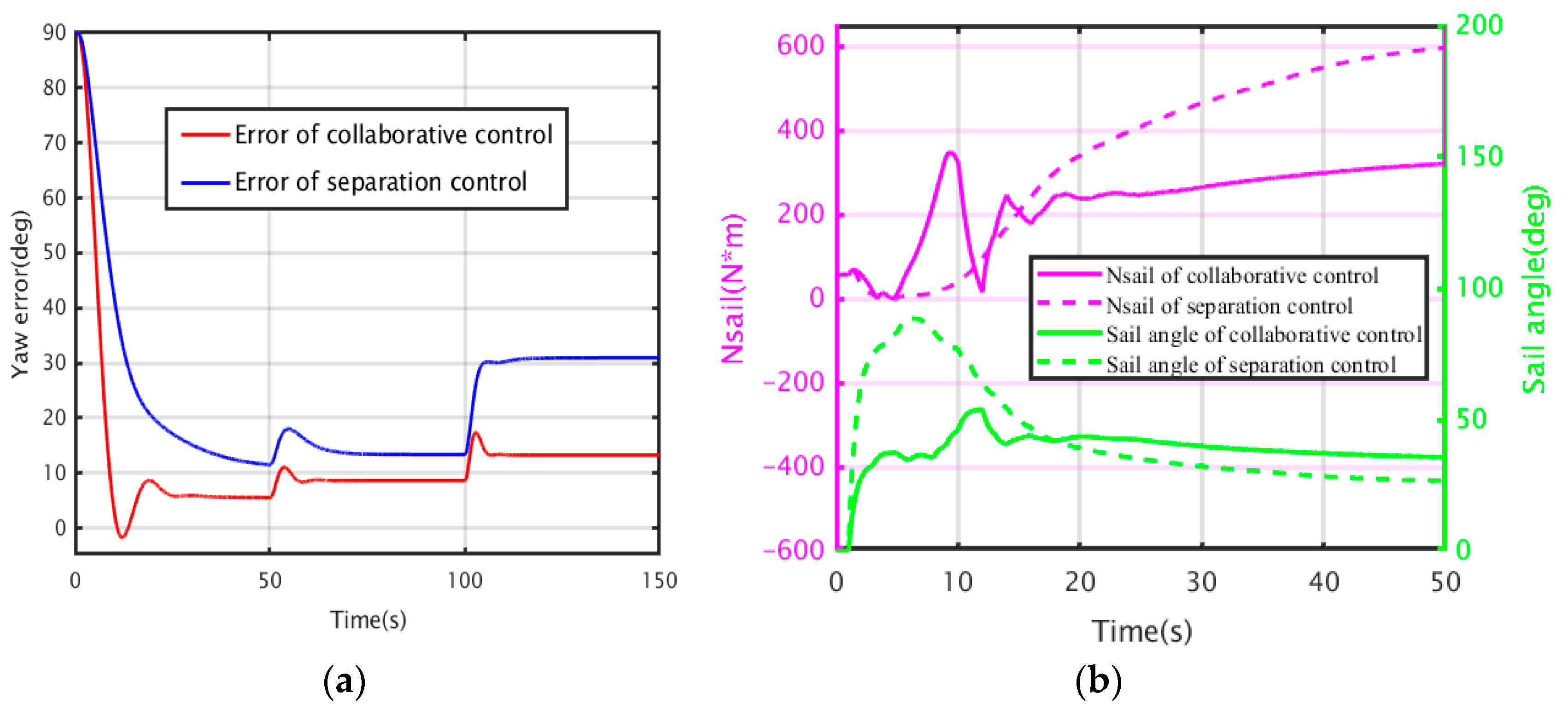From Figure 5a, we can see that the yaw angle of collaborative control converges faster in 0–50 s with a wind speed of 3 m/s, the yaw angle converges in about 24 s and the steady-state error is 6.07°. However, the separation control converges to a stable yaw angle at around 47 s, and the steady-state error is 11.65°. The steady-state error of the yaw angle under different wind speeds is shown in

Table 3. Yaw error of the collaborative control and separation control.

Yaw Error	Collaborative Control (deg)	Separation Control (deg)
3 m/s	6.07	11.65
5 m/s	8.63	13.36
8 m/s	13.25	30.91

below. It is proved that the collaborative control considering the roll angle has a better yaw angle control effect than the separation control without considering the roll.

It can be seen from Figure 5a that in the 90° sidewind sailing, the dynamic characteristics of collaborative control are better than that of separate control for yaw angle control. This is because the sail also takes part in the turning action of the sailboat during the collaborative control. However, the separation control can only output the sail angle of the optimal thrust according to the real-time relative wind angle, which does not help the sailboat to turn. In the Figure 5b, $N_{sail}$ represents the yaw moment generated by the wind acting on the sail. As shown in Figure 5b, the $N_{sail}$ controlled by the collaborative control is larger than that of the separated control at 0~12 s. The average sail yaw moment $N_{sail}$ of the collaborative control is 117.04 N*m, while the average sail yaw moment $N_{sail}$ of the separated control is 29.68 N*m. By $\left(I_{zz}+J_{zz}\right)\ddot{\psi }=N_{hull}+N_{rudder}+N_{sail}$, it can be seen that the acceleration of the yaw angle at 0~12 s for the collaborative control is greater than that of the separation control. It shows that the sail in the collaborative control participates in the steering action of the sailboat and provides the moment for the sailboat to steer, which contributes to the rapid convergence of the yaw angle to some extent.

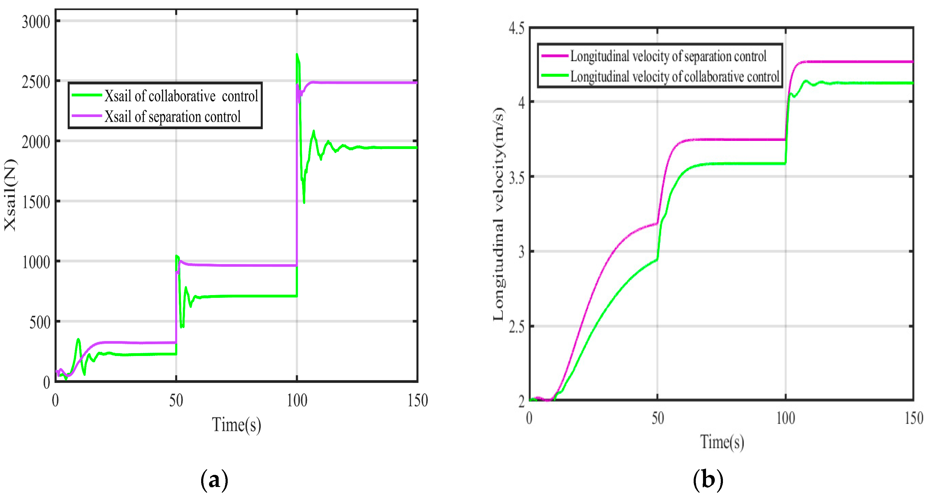
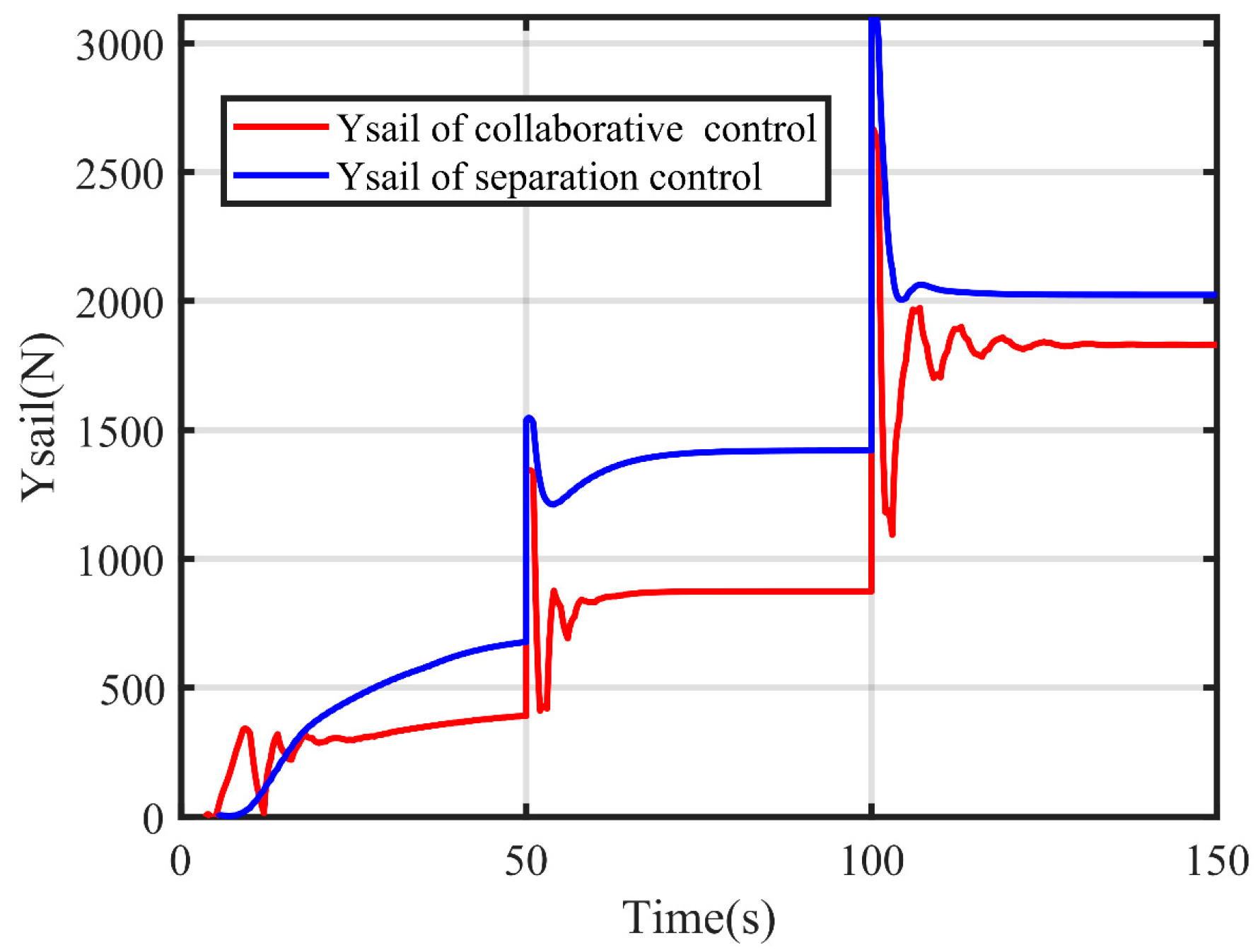
As seen in Figure 6a,b, the longitudinal velocities of the collaborative control and the separation control keep increasing and do not converge within 0~50 s, and the difference between the longitudinal thrust $X_{sail}$ of the two sails is not significant at this time. At 50~100 s, the longitudinal thrust $X_{sail}$ of the separated control is 963.65 N and the longitudinal thrust $X_{sail}$ of the collaborative control is 708.77 N. The longitudinal thrust of the collaborative control is reduced by 26.4% compared with the separated control. The longitudinal velocity of the separated control converges to 3.75 m/s and the longitudinal velocity of the collaborative control converges to 3.58 m/s. The longitudinal velocity of the collaborative control is reduced by 4.5% compared with the separated control. At 100~150 s, the longitudinal thrust $X_{sail}$ of the separated control is 2484.57 N and the longitudinal thrust $X_{sail}$ of the collaborative control is 1943.18 N. The longitudinal thrust of the collaborative control is reduced by 21.7% compared to the separated control. The longitudinal velocity of the separation control converges to 4.27 m/s, the longitudinal velocity of the cooperative control converges to 4.12 m/s and the velocity loss is only 3.5%. Although the collaborative control sacrifices part of the longitudinal thrust $X_{sail}$ by increasing the sail angle, the longitudinal speed loss is smaller than the longitudinal thrust loss due to the reduction of additional drag $X_{hull}$ brought by the reduction of roll angle.

4.2. Comparison of Sail–Rudder Collaborative and Separation Lateral Shift

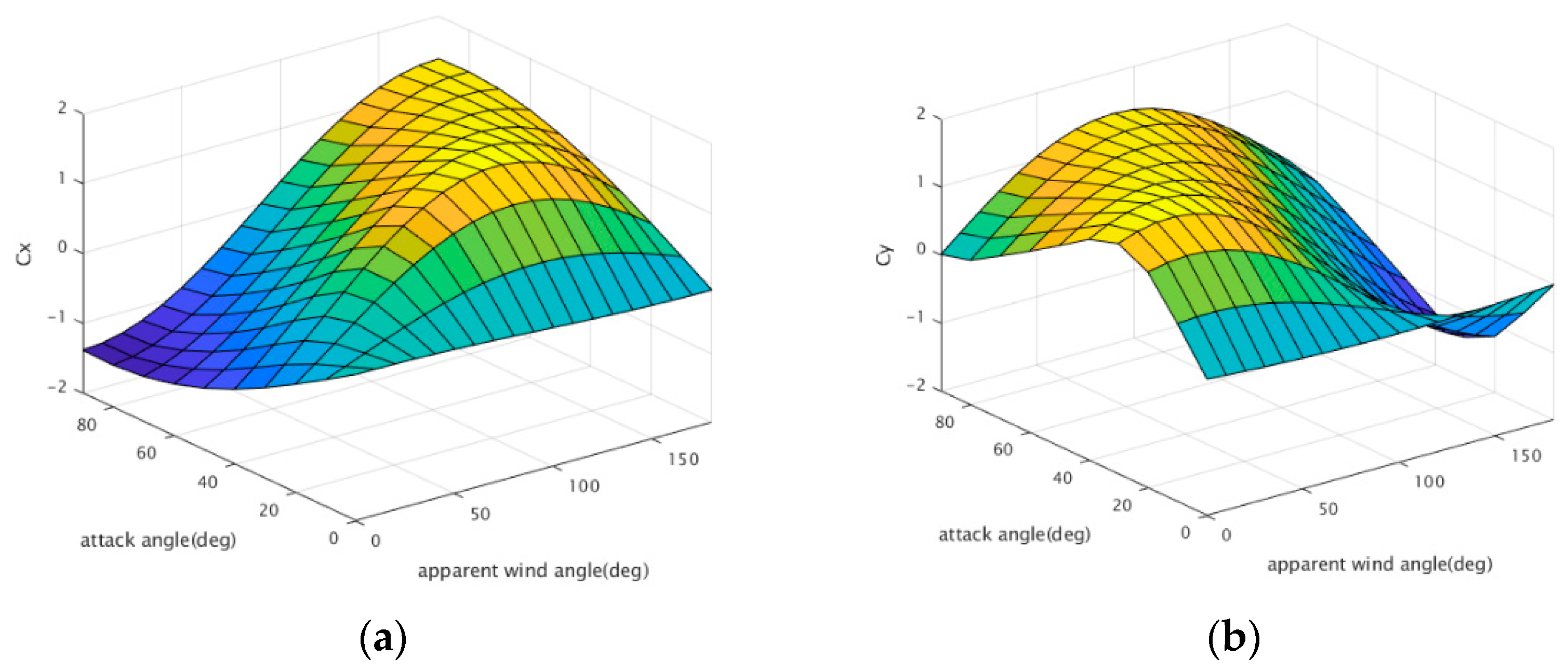
In the sailing of the unmanned sailboat, the force of wind can be decomposed into the transverse and longitudinal directions of the hull, so the sailboat must move sideways. This situation is especially obvious when sailing in the side wind, which will make the sailboat deviate from the predetermined path. This is also the main reason for the poor tracking accuracy of unmanned sailboats. In collaborative control, since the set sail angle does not follow the optimal thrust sail angle, the sail angle will be greater than the optimal thrust sail angle. At the same wind angle, the angle of attack will decrease when the sail angle increases. The reduction of the angle of attack will reduce the lateral displacement force in addition to the longitudinal driving force, which can reduce the lateral displacement to a certain extent.

The forward thrust of the sail can be expressed as $X_{sail}=C_x{\cos }^2\varphi *\frac{1}{2}{\rho }_a{U}_A^2{S}_A$, and the lateral force of the sail can be expressed as $Y_{sail}=C_y{\cos }^2\varphi \frac{1}{2}{\rho }_a{U}_A^2{S}_A$. Coefficients $C_x$ and $C_y$ are related to the angle of attack and the relative wind angle, and the relationship between them is shown in the Figure 7.

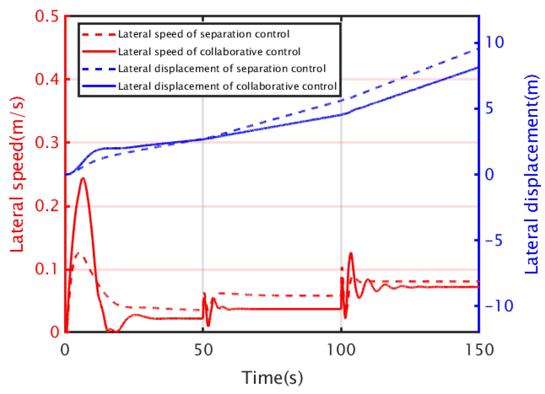
The lateral speed and lateral displacement for the two control methods are shown in Figure 8, and the specific values are shown in

Table 4. Lateral speed and lateral displacement of the collaborative control and separation control.

Control Method	Lateral Speed (m/s)	Lateral Displacement (m)
collaborative control	0.054	8.152
separation control	0.064	9.586

.

This proves that the collaborative control can limit the lateral displacement of the unmanned sailboat to a certain extent. The reason for this can be seen in Figure 9, where the lateral thrust of the separation control is always greater than that of the collaborative control.

4.3. Four-Point Navigation Comparison Simulation

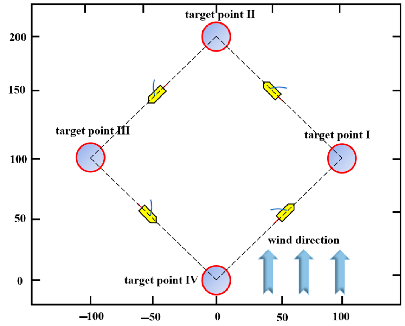
The simulation compares the collaborative control and separation control in four-point navigation. As shown in Figure 10, four target points are set, and the sailboat starts at (0,0) and passes target point I:(100,100), target point II:(0,200), target point III:(−100,100) and target point IV:(0,0) in turn. The LOS guidance method is used for the yaw angle guidance. It is stipulated that when the sailboat enters the area with the target point as the center and 10 m as the radius, it is regarded as reaching the target point and starts to turn to the next target point for navigation. The initial yaw angle of the unmanned sailboat is 315°. The initial roll angle is 0°. The initial longitudinal speed is u = 2 m/s. The wind direction and wind speed are as follows: ${\alpha }_{tw}={270}^{°}$ and $V_{tw}=3 \mathrm{m}/\mathrm{s}$. The collaborative control weights are set as follows: $Q_y=diag\left(1,2\right) \mathrm{and} Q_u=diag\left(0.1,1\right)$. The separation control weights are set as follows: $Q_y=\left[1\right] \mathrm{and} Q_u=diag\left(0.1,1\right)$.

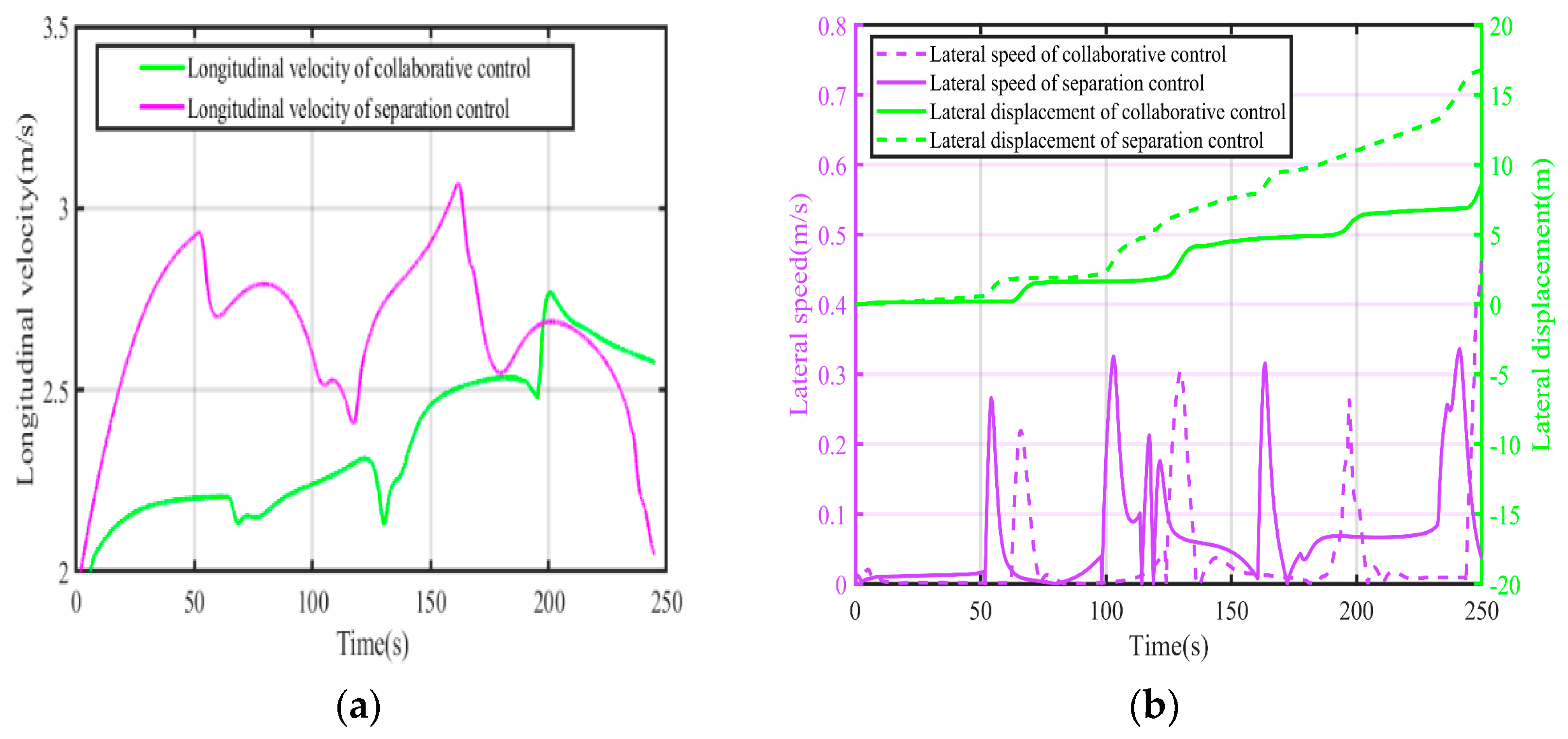
The longitudinal velocity comparison between collaborative control and separation control during four-point navigation is shown in Figure 11a. The average longitudinal velocity of separation control is 2.65 m/s, and the average longitudinal velocity of collaborative control is 2.35 m/s, with a 12% velocity loss.

As shown in Figure 11b, during the whole navigation process, the total lateral shift of separation control is 16.74 m, while the total lateral shift of collaborative control is 8.46 m. As the lateral shift is smaller, the collaborative control reduces the lateral deviation from the target path and achieves a better path tracking effect.

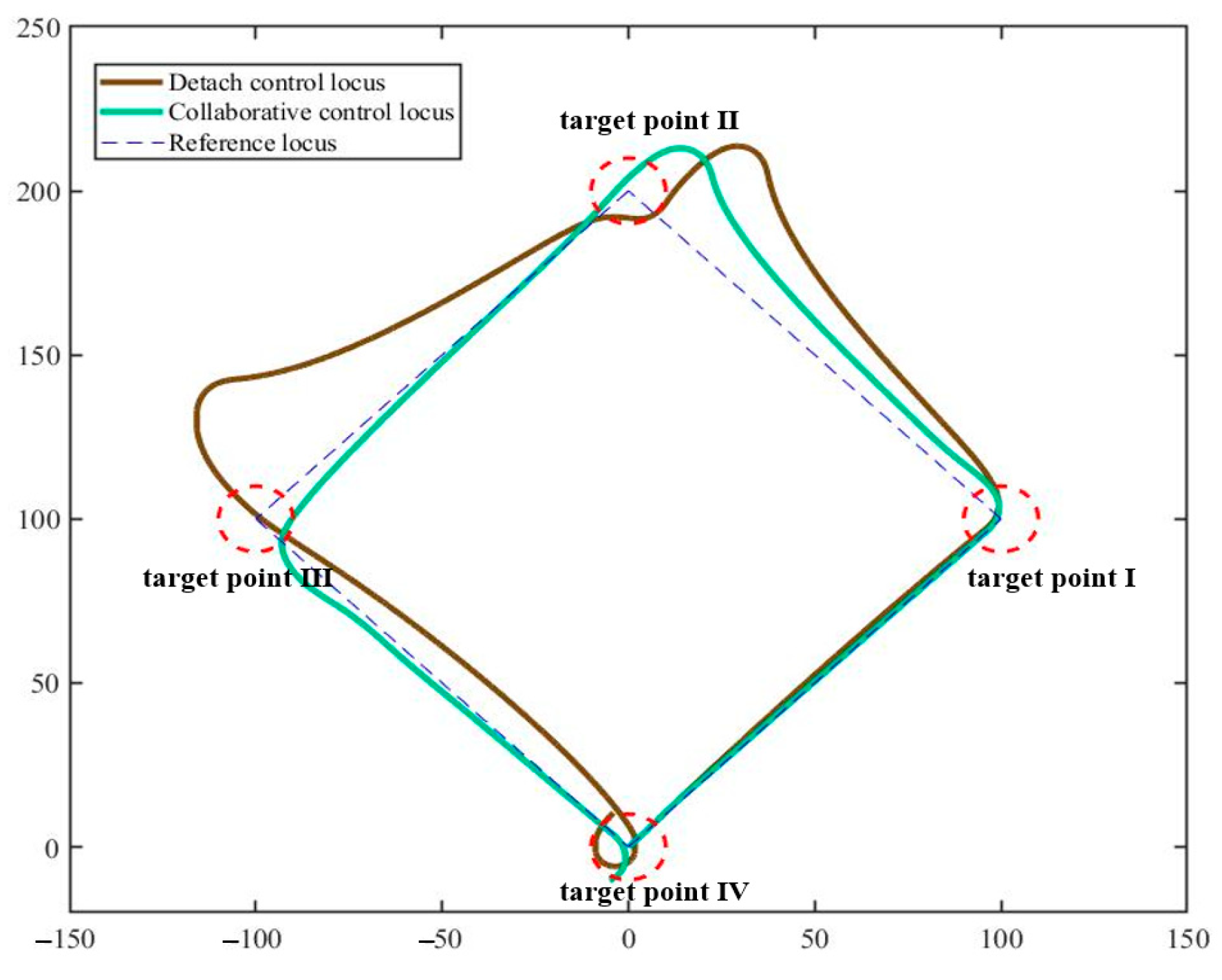
The four-point navigation path diagram is shown in Figure 12. The target area is marked by a red dashed circle. The target path is marked by a blue dashed line. The green solid line is the path navigated by the collaborative control algorithm. The brown solid line is the path navigated by the separation control algorithm. It can be clearly seen that the collaborative control can obtain more accurate path tracking compared with the separation control. The first path is defined as from target point IV to target point I. The second path is defined as from target point I to target point II. The third path is defined as from target point II to target point III. The fourth path is defined as from target point III to target point IV. The straight-line distance between the real-time path point and the target path of the sailing boat is defined as the side-shift deviation, and the maximum side-shift deviation and average side-shift deviation of the sailing boat in the four segments of the path are calculated. The results are shown in

Table 5. Maximum deviation of the collaborative control and separation control.

Maximum Deviation	Collaborative Control (m)	Separation Control (m)
the first path	0.573	1.791
the second path	21.243	32.454
the third path	5.985	37.041
the fourth path	4.626	8.728

and

Table 6. Average deviation of the collaborative control and separation control.

Average Deviation	Collaborative Control (m)	Separation Control (m)
the first path	0.293	1.207
the second path	8.886	15.871
the third path	1.969	16.796
the fourth path	1.904	6.019

.

It can be seen that the maximum and average deviations of separation control are larger than those of collaborative control in each segment of the path, mainly because collaborative control has better yaw control and a better side-shift limiting effect than separation control.

The time to reach the target point using the collaborative control and the separation control is shown in

Table 7. Time of arrival at each point of the collaborative control and separation control.

Time Of Arrival	Separation Control (s)	Collaborative Control (s)
target point Ⅰ	51.35	61.22
target point Ⅱ	116.88	135.30
target point Ⅲ	176.87	193.72
target point Ⅳ	231.96	243.10

. Since the separation control has a longitudinal speed advantage compared with the collaborative control, the collaborative control is 11.14 s slower than the separation control at the end of the four-point navigation, which is a loss of 4.8%. The speed advantage of the separation control is not obvious, and it is worthwhile to lose a little speed for more accurate path tracking.

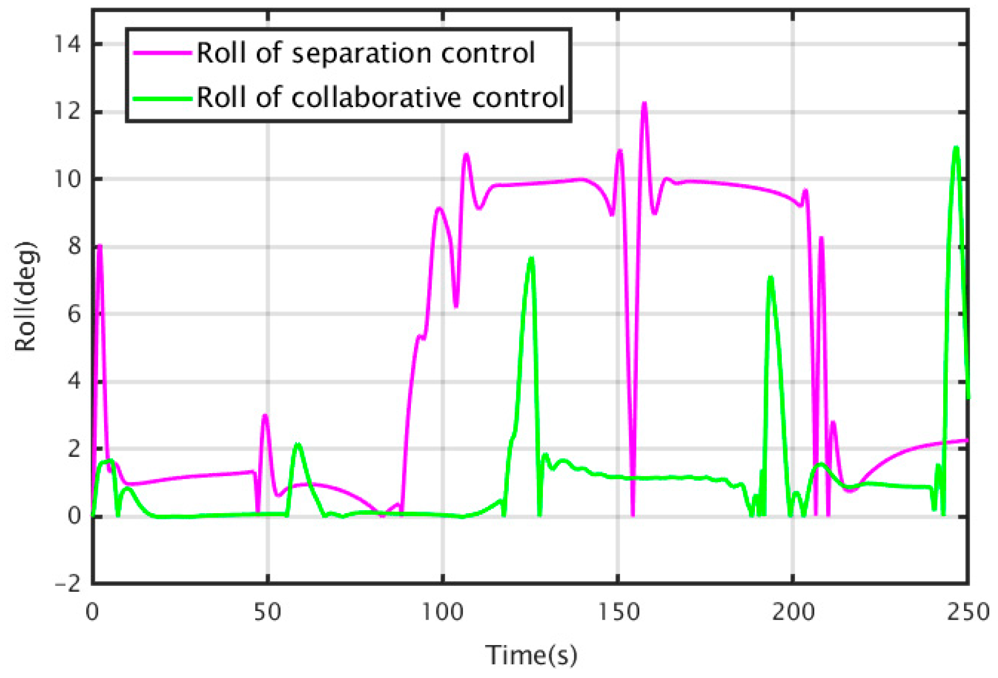
The roll angle of the two control methods are shown in

Table 8. Maximum roll angle and average roll angle of the collaborative control and separation control.

Control Method	Maximum Roll Angle (deg)	Average Roll Angle (deg)
separation control	12.298	5.042
collaborative control	10.975	1.103

.

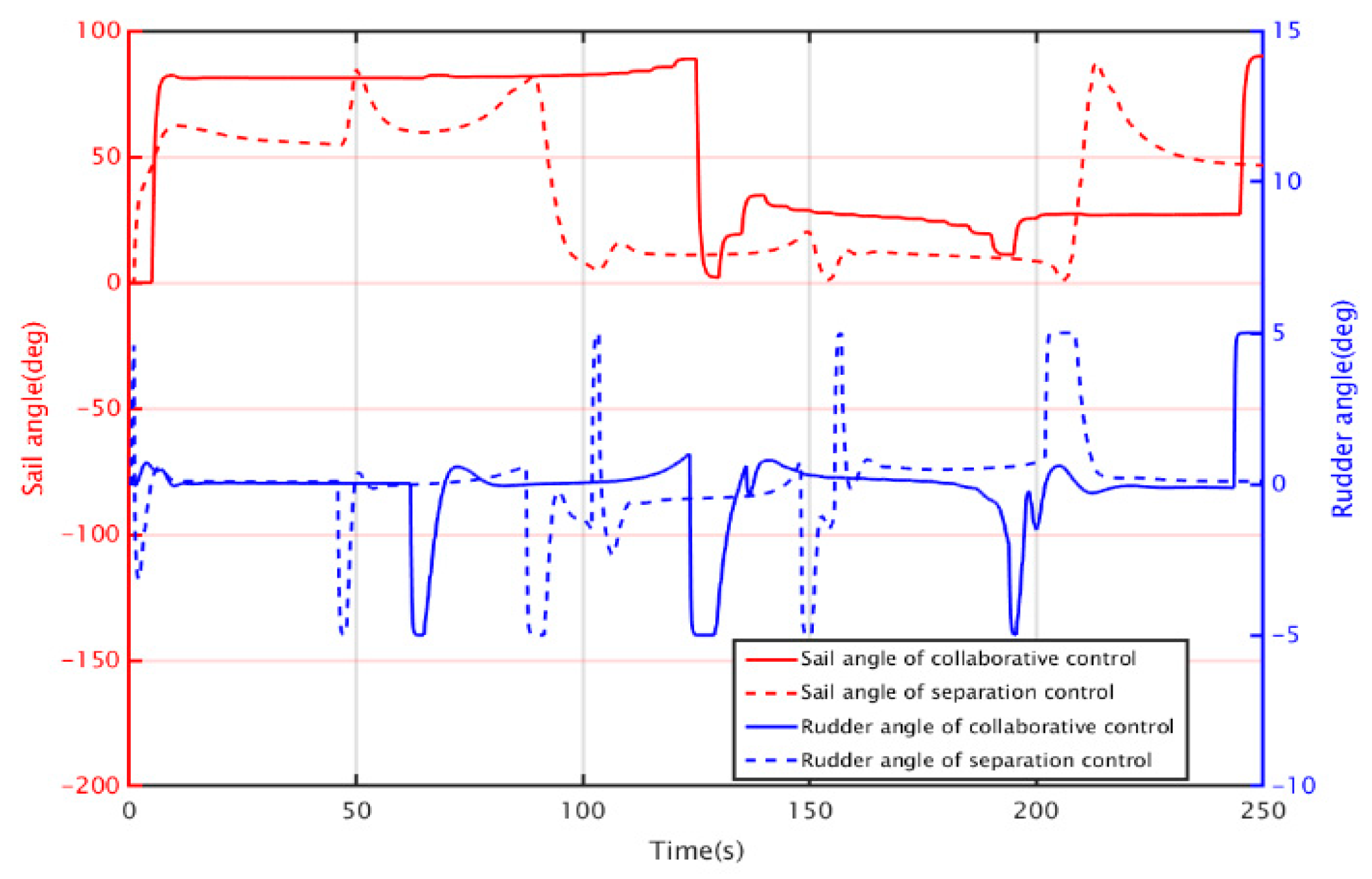
From Figure 13, it can be seen that the roll angle of the collaborative control is basically smaller than that of the separation control during the whole sailing process. It can be seen from Figure 14 that the sail angle of collaborative control is greater than the sail angle of separate control during the whole navigation process. This is because the separation control uses the optimal thrust sail angle. In order to achieve better yaw angle control and roll angle limitation, the collaborative control increases the sail angle based on the optimal thrust sail angle. The angle of attack decreases with the increase in sail angle, resulting in the reduction of the lateral component of the sail and the reduction of the roll moment. Therefore, the collaborative control has achieved a better control effect with smaller roll angle and better lateral displacement limitation.

5. Conclusions

This paper considers the coupling relationship between the sail and rudder of the unmanned sailboat and proposes a collaborative control method of the sail and rudder of the unmanned sailboat based on MPC. This algorithm can control the yaw angle and limit the roll angle at the same time. First of all, the four-degree-of-freedom kinematics and dynamics model of the unmanned sailboat is established, and the problem of heading angle and heeling angle control is transformed into an optimization problem with constraints. Secondly, considering input constraints and state constraints, the optimization problem is transformed into a standard convex quadratic programming problem that can be calculated online. Finally, when the unmanned sailboat reaches a new state, the optimal input at the next moment is recalculated according to the current state and expected state, and the rolling optimization is carried out according to this cycle. By comparing the collaborative control with the separation control through simulation experiments, it is proved that the collaborative control can achieve a smaller steady-state error of the yaw angle and smaller roll angle than the separation control. Collaborative control can also achieve smaller side shift limitation and a better path tracking effect in four-point navigation.