A Novel Robust IMM Filtering Method for Surface-Maneuvering Target Tracking with Random Measurement Delay

Abstract

A proper filtering method for jump Markov system (JMS) is an effective approach for tracking a maneuvering target. Since the coexisting of heavy-tailed measurement noises (HTMNs) and one-step random measurement delay (OSRMD) in the complex scenarios of the surface maneuvering target tracking, the effectiveness of typical interacting multiple model (IMM) techniques may decline severely. To solve the state estimation problem in JMSs with HTMN and OSRMD simultaneously, this article designs a novel robust IMM filter utilizing the variational Bayesian (VB) inference framework. This algorithm models the HTMNs as student’s t-distribuitons, and presents a random Bernoulli variable to describe the OSRMD in JMSs. By transforming measurement likelihood function form from weighted summation to exponential product, this paper constructs hierarchical Gaussian state space models. Then, the state vectors, random Bernoulli vairable, and model probability are inferred jointly according to VB inference. The surface maneuvering target tracking simulation example result indicates that the presented IMM filter achieves superior target state estimation accuracy among existing IMM filters.

1. Introduction

State estimation is an important topic in maneuvering target tracking of traditional ships and surface autonomous ships. As a minimum mean square error estimator, the Kalman filter (KF) provides the optimal state estimation method for a linear Gaussian system (The abbreviations are summarized in

Table 1. Definitions of notations in this paper.

Notation	Definition	Notation	Definition
VB	Variational Bayesian	HGSSM	Hierarchical Gaussian state space model
KF	Kalman filter	OSRMD	One-step random measurement delay
PDF	Probability density function	$N\left(·;\overline{\mu },P\right)$	Gaussian distribution,
JMS	Jump Markov system		$\overline{\mu }$-mean vector, P-scale matrix
STD	student’s t-distribution	$St\left(·;\overline{\mu },P,v\right)$	Student’s t-distribution,
RBV	Random Bernoulli variable		$\overline{\mu }$-mean vector, P-scale matrix,
KLD	Kullback-Leibler divergence		v-degree of freedom parameter
$E\left[·\right]$	Expectation computation	$G\left(·;a,b\right)$	Gamma distribution,
$tr\left(·\right)$	Trace operation		a-shape parameter,
HTMN	Heavy-tailed measurement noise		b-rate parameter

). However, the system nonlinearity and system model uncertainty in jump Markov systems (JMSs) may lead to the KF’s performances degrading dramatically. Additionally, the KF assumes that the measurement noises obey Gaussian distributions and that all measurements need to arrive in time. Both aspects may affect the filtering accuracy significantly when these assumptions are not satisfied. Thus, the extension for the KF under various assumptions has attracted considerable attention on account of its widely applied in engineering, for example, targets tracking, signal processing, integrated navigation, fault diagnosis, ect. [1,2,3,4,5,6].

The surface maneuvering target tracking is a problem of state estimation in JMSs. Since the state estimation in JMSs is well-known computational intractability and nondeterministic polynomial difficult, it is hard to find an optimal solution [7]. In the past few decades, some sub-optimal solutions were presented, for example, the interacting multiple model (IMM) approach [8], pseudo-Bayesian technique [9], particle filter [10], etc. Among these methods, the IMM approach is one of the most efficient since it reasonably balances the estimation performances and the computation complexity. In the process of IMM technique development, many researchers contributed remarkable achievements. The stability and performances of the IMM filter are analyzed by [11,12]. A series of executable pseudocode is provided in [13]. IMM algorithms are widely used in various practical engineering [14,15,16].

The typical IMM filters parallelly perform a bank of KFs to estimate mode-conditional system state and probability at each cycle. The weighted sum of sub-filter outputs obtains the final state estimates [17]. An effective method to develop the performances of sub-filters (KFs) is the variational Bayesian (VB) inference, which implements approximations for the conjugate exponential model with acceptable computational costs [18]. Based on the combination of VB theory and the KF, the development of the KF has made significant progress and remarkable achievements [19,20,21,22]. Extended to IMM filters for the state estimation in JMSs, some VB-based IMM methods were designed in past few years. Ref. [23] presented an IMM filter to adaptively estimate the unknown process and measurement noise covariance matrices in JMS. The authors selected the conjugate prior distribution of noise covariance matrix as the inverse-Wishart distribution, the conditional system state vectors and the noise parameters can be estimated simultaneously by VB inference. This method achieved remarkable estimation accuracy when the noise covariances were unknown. However, this technique requires linear Gaussian systems, and the measurements need to be arrived in time, which is usually not satisfied in actual tracking scenarios affected by measurement outliers and communication channel latency.

Aiming to solve state estimation problems in JMSs with measurement outliers, Ref. [24] modeled the measurement noises as students’ t-distributions (STDs), and estimated the system states and mode probabilities jointly by VB inference. Compared with the typical IMM algorithm, the estimation performance was significantly developed. Ref. [25] developed the IMM filter in [24] by reasonably selecting the conjugate prior distributions of covariances and degree of freedom parameters as inverse Wishart and Gamma distributions, respectively. The state vectors and the degree of freedom parameters were inferred simultaneously by VB method. This algorithm improved the estimation accuracy and can be utilized for nonlinear JMSs. The methods mentioned in [24,25] show superior estimation accuracy in the scenarios of state estimation in JMSs containing heavy-tailed measurement noises (HTMNs). However, the performances of these approaches may lose efficacy when the random measurement delay happens since they assume the measurements can be obtained in real-time. To deal with the one-step random measurement delay (OSRMD), Ref. [26] designed a particle filter by defining two variables to extend the original system state vector. This filter can effectively handle the systems with delayed measurements. Although this algorithm provided a solution to measurement delay and achieved satisfactory estimation accuracy, the particle filters have problems of high computational burden and curse of dimensionality. Ref. [27] proposed a Gaussian approximate filter with OSRMD, and measurement noise vectors are inferred by the Bayesian rules. Ref. [28] developed the KF to deal with the OSRMD in nonlinear systems. In this method, the authors utilized a random Bernoulli variable (RBV) to describe the random measurement delay, and the system states were inferred by the VB technique. However, these methods failed to deal with the HTMN and system model jumping problems in JMSs. In complex JMSs engineering applications, the HTMNs and random measurement delay often exist simultaneously. It is necessary to propose a more general IMM filter for HTMNs coexist with random measurement delay.

This article designs a novel robust IMM filter to deal with the filtering problems in JMSs with HTMN and OSRMD. The HTMN and the OSRMD in JMSs are reasonably modeled in the designed filter. By transforming the measurement likelihood function to a new form, this algorithm constructed a new hierarchical Gaussian state space model (HGSSM). According to the VB inference, the state vectors, model probability, RBVs, and distribution parameters are inferred simultaneously. Target tracking experiment validates that the presented approach has better performance than existing IMM approaches.

The main contribution of our work is summarized as follows:

• The one-step predictive probability density function (PDF) and HTMN are assumed to obey Gaussian and STDs, respectively. This paper presents an RBV to characterize the OSRMD in JMSs. Aiming to introduce the VB method directly, this article converts measurement likelihood function form from weighted summation to exponential product, and constructs the HGSSM.
• To address the coupled state vectors and the noise covariance matrices, a novel IMM filter is designed by combining the VB theory with IMM method. In measurement update part, the mode conditional posterior PDFs are approximated recursively. The state vectors, RBVs, model probabilities, and unknown parameters are estimated through VB technique. Then, the final estimates are obtained by the weighted sum of sub-filters.
• Four parts of the surface target tracking simulation indicate that the presented method outperforms existing IMM filters on estimation accuracy. The presented algorithm provides a robust solution to the filtering problem in the scenarios of HTMNs coexisting with OSRMD.

The rest parts of this paper can be arranged as the following sections. Section 2 provides the problem statement. We construct a new HGSSM in Section 3. Furtherly, we summarize the derivations of our designed IMM method in Section 4. The performances of exsiting IMM algorithms and the proposed are verified in Section 5. Finally, the conclusions of this paper is in Section 6.

2. Problem Statement

Considering a state-space model of nonlinear jump Markov system:

$$\begin{array}{cc}\hfill & x_s=f_{s-1}\left(x_{s-1},M_{s-1}\right)+g_{s-1},s\ge 1\hfill \end{array}$$

(1)

$$\begin{array}{cc}\hfill & z_s=h_s\left(x_s,M_s\right)+{\epsilon }_s,s\ge 1\hfill \end{array}$$

(2)

$$\begin{array}{cc}\hfill & y_s=\left\{\begin{array}{cc}\left(1-{\sigma }_s\right)z_s+{\sigma }_s{z}_{s-1},\hfill & s>1\\ z_s,\hfill & s=1\end{array}\right.\hfill \end{array}$$

(3)

where s is time index, $x_s\in {\mathbb{R}}^n$ is the system state vector, $z_s\in {\mathbb{R}}^m$ and $y_s\in {\mathbb{R}}^m$ denote the ideal and real measurement vectors, m and n are their dimension numbers. $f_{s-1}\left(·\right)$ and $h_s\left(·\right)$ refer to the process function and measurement function. We denote $f_{s-1}\left(x_{s-1},M_{s-1}\right)$ as $f_{s-1}^i\left(x_{s-1}\right)$ and $h_s\left(x_s,M_s\right)$ as $h_s^i\left(x_s\right)$ conditioned on $M_s=i$, respectively. The system mode $M_s$ indicates the state of the Markov chains. It selects a value from a limited set $\left\{1,2,3,\dots ,k\right\}$ according to the transition probability matrix $T={\left[{\lambda }_{ji}\right]}_{k\times k}$, which satisfies the equations as follows:

$$\begin{array}{cc}\hfill & {\lambda }_{ji}\stackrel{\Delta }{=}P\left\{M_s=i\left|M_s=j\right.\right\}\hfill \end{array}$$

(4)

$$\begin{array}{cc}\hfill & \underset{i=1}{\overset{k}{\Sigma }}{\lambda }_{ji}=1\hfill \end{array}$$

(5)

$g_{s-1}$ represents the Gaussian process noise vector with nominal covariance matrix $Q_s$, while ${\epsilon }_s$ refers to the HTMN vector caused by measurement outliers with nominal covariance matrix $R_s$. $y_s\in {\mathbb{R}}^m$ denotes the real random delayed measurement vector. The RBV ${\sigma }_s\in \left\{0,1\right\}$ with corresponding probability can be defined as follows:

$$\begin{array}{cc}\hfill & p\left({\sigma }_s=1\right)={\phi }_s\hfill \end{array}$$

(6)

$$\begin{array}{cc}\hfill & p\left({\sigma }_s=0\right)=1-{\phi }_s\hfill \end{array}$$

(7)

where ${\phi }_s\in \left(0,1\right)$ denotes the probability of OSRMD. Note that random variables $x_s$, ${\sigma }_s$, $g_{s-1}$, and $r_s$ are independent of each others.

Utilizing Equation (3) and Equations (6) and (7), the measurement likelihood PDF is as follows:

$$\begin{array}{cc}\hfill & p\left(y_s\left|x_s,x_{s-1}\right.,M_s=i\right)=\sum _{{\sigma }_s=0}^{1}p\left(y_s,{\sigma }_s\left|x_s,x_{s-1},M_s=i\right.\right)\hfill \\ \hfill & =p\left({\sigma }_s=1\right)p\left(y_s\left|x_s,x_{s-1},{\sigma }_s=1\right.,M_s=i\right)+p\left({\sigma }_s=0\right)p\left(y_s\left|x_s,x_{s-1},{\sigma }_s=0\right.,M_s=i\right)\hfill \\ \hfill & ={\phi }_{s}p\left(y_s\left|x_s,x_{s-1}\right.,{\sigma }_s=1,M_s=i\right)+\left(1-{\phi }_s\right)p\left(y_s\left|x_s,x_{s-1},{\sigma }_s=0,M_s=i\right.\right)\hfill \end{array}$$

(8)

Utilizing Equations (2) and (3) yields

$$\begin{array}{cc}\hfill & p\left(y_s\left|x_s,x_{s-1}\right.,{\sigma }_s=1,M_s=i\right)=p_{{\epsilon }_{s-1}}\left[y_s-h_{s-1}\left(x_{s-1}\right)\right]\hfill \end{array}$$

(9)

$$\begin{array}{cc}\hfill & p\left(y_s\left|x_s,x_{s-1}\right.,{\sigma }_s=0,M_s=i\right)=p_{{\epsilon }_s}\left[y_s-h_s\left(x_s\right)\right]\hfill \end{array}$$

(10)

In Equation (8), replaced by Equations (9) and (10), we can obtain:

$$\begin{array}{c}\hfill p\left(y_s\left|x_s,x_{s-1}\right.,M_s=i\right)={\phi }_s{p}_{{\epsilon }_{s-1}}\left[y_s-h_{s-1}\left(x_{s-1}\right)\right]+\left(1-{\phi }_s\right)p_{{\epsilon }_s}\left[y_s-h_s\left(x_s\right)\right]\end{array}$$

(11)

However, the measurement likelihood PDF in Equation (11), which is formulated by a weighted sum form, has neither conjugate property nor closed property. Therefore, it is not easy to introduce the VB technique directly. Aiming at this difficulty, in the next section, the weighted sum form of measurement likelihood PDF is converted to exponential multiplication, which can be further utilized to design a novel adaptive estimation method for JMSs.

3. Construction of the HGSSM

3.1. Measurement Likelihood PDF Convertion

The relationship between RBV ${\sigma }_s$ with fixed delay probability can be seen in Equations (6) and (7). The probability mass function $p\left({\sigma }_s\left|{\phi }_s\right.\right)$ is defined as the following formula:

$$\begin{array}{c}\hfill p\left({\sigma }_s\right)={\left(1-{\phi }_s\right)}^{\left(1-{\sigma }_s\right)}{{\phi }_s}^{{\sigma }_s}\end{array}$$

(12)

according to Equations (11) and (12), reformulating Equation (8) by:

$$\begin{array}{cc}\hfill & p\left(y_s\left|x_s,x_{s-1},M_s=i\right.\right) =\sum _{{\sigma }_s=0}^{1}p\left(y_s,{\sigma }_s\left|x_s,x_{s-1},M_s=i\right.\right)\hfill \\ \hfill & =\sum _{{\sigma }_s=0}^1{\left({\phi }_s\right)}^{{\sigma }_s}{p}_{{\epsilon }_{s-1}}{\left(y_s-h_{s-1}\left(x_{s-1}\right)\right)}^{{\sigma }_s}{\left(1-{\phi }_s\right)}^{\left(1-{\sigma }_s\right)}{p}_{{\epsilon }_s}{\left(y_s-h_s\left(x_s\right)\right)}^{\left(1-{\sigma }_s\right)}\hfill \\ \hfill & =\sum _{{\sigma }_s=0}^{1}p\left({\sigma }_s\right)p_{{\epsilon }_{s-1}}{\left(y_s-h_s\left(x_s\right)\right)}^{{\sigma }_s}{p}_{{\epsilon }_s}{\left(y_s\right)}^{\left(1-{\sigma }_s\right)}\hfill \end{array}$$

(13)

then, transforming the conditional measurement likelihood PDF to exponential product form:

$$\begin{array}{c}\hfill p\left(y_s\left|x_s,x_{s-1},{\sigma }_s\right.\right)={\left[p_{{\epsilon }_{s-1}}\left(y_s-h_{s-1}\left(x_{s-1}\right)\right)\right]}^{{\sigma }_s}{\left[p_{{\epsilon }_s}\left(y_s-h_s\left(x_s\right)\right)\right]}^{\left(1-{\sigma }_s\right)}\end{array}$$

(14)

Equation (14) can be also denoted by the formula as follows:

$$\begin{array}{c}\hfill p\left(y_s\left|{\eta }_s,{\sigma }_s\right.\right)={\left[p_{{\epsilon }_{s-1}}\left(y_s-h_{s-1}\left(x_{s-1}\right)\right)\right]}^{{\sigma }_s}{\left[p_{{\epsilon }_s}\left(y_s-h_s\left(x_s\right)\right)\right]}^{\left(1-{\sigma }_s\right)}\end{array}$$

(15)

where the extended state vector ${\eta }_s={\left[\begin{array}{cc}{x}_s^T& x_{s-1}^T\end{array}\right]}^T$.

3.2. Prior PDFs Selection

First of all, the one-step predictive PDF of the extended system state ${\eta }_s$ is formulated by

$$\begin{array}{c}\hfill p\left({\eta }_s\left|y_{1:s-1}\right.\right)=N\left({\eta }_s;{\widehat{\eta }}_{s\left|s-1\right.},P_{s\left|s-1\right.}^{\eta \eta }\right)\end{array}$$

(16)

where ${\widehat{\eta }}_{s\left|s-1\right.}$ represents the predicted mean vector, $P_{s\left|s-1\right.}^{\eta \eta }$ refers to the predicted covariance matrix, and they are expressed by:

$$\begin{array}{cc}\hfill & {\widehat{\eta }}_{s\left|s-1\right.}={\left[\begin{array}{cc}{\widehat{x}}_{s\left|s-1\right.}^T& {\widehat{x}}_{s-1\left|s-1\right.}^T\end{array}\right]}^T\hfill \end{array}$$

(17)

$$\begin{array}{cc}\hfill & P_{s\left|s-1\right.}^{\eta \eta }=\left[\begin{array}{cc}{P}_{s\left|s-1\right.}& P_{s-1,s\left|s-1\right.}\\ {\left(P_{s-1,s\left|s-1\right.}\right)}^T& P_{s-1\left|s-1\right.}\end{array}\right]\hfill \end{array}$$

(18)

where ${\widehat{\eta }}_{s\left|s-1\right.}$, $P_{s\left|s-1\right.}$, and $P_{s-1,s\left|s-1\right.}$ can be calculated by the standard Gaussian approximate filter [29], i.e.,

$$\begin{array}{cc}\hfill & {\widehat{x}}_{s\left|s-1\right.}=\int f_{s-1}^i\left(x_{s-1}\right)N\left(x_{s-1};{\widehat{x}}_{s-1\left|s-1\right.},P_{s-1\left|s-1\right.}\right)d{x}_{s-1}\hfill \end{array}$$

(19)

$$\begin{array}{cc}\hfill & P_{s\left|s-1\right.}=\int f_{s-1}^i\left(x_{s-1}\right)f_{s-1}^{i\left(T\right)}\left(x_{s-1}\right)N\left(x_{s-1};{\widehat{x}}_{s-1\left|s-1\right.},P_{s-1\left|s-1\right.}\right)d{x}_{s-1}\hfill \end{array}$$

(20)

$$\begin{array}{cc}\hfill & P_{s-1,s\left|s-1\right.}=\int x_{s-1}{f}_{s-1}^{i\left(T\right)}\left(x_{s-1}\right)N\left(x_{s-1};{\widehat{x}}_{s-1\left|s-1\right.},P_{s-1\left|s-1\right.}\right)d{x}_{s-1}-{\widehat{x}}_{s-1\left|s-1\right.}{\widehat{x}}_{s\left|s-1\right.}^T\hfill \end{array}$$

(21)

Secondly, in the aspects of processing the measurement noises, since the STD has heavier tails compared with Gaussian distribution and is more robust to outlier [30,31,32], STD is selected to model HTMN, i.e.,

$$\begin{array}{cc}\hfill & p\left({\epsilon }_{s-1}\right)=St\left({\epsilon }_{s-1};0,R_{s-1},{\tau }_{s-1}\right)\hfill \end{array}$$

(22)

$$\begin{array}{cc}\hfill & p\left({\epsilon }_s\right)=St\left({\epsilon }_s;0,R_s,{\tau }_s\right)\hfill \end{array}$$

(23)

where the $p\left({\epsilon }_{s-1}\right)$ and $p\left({\epsilon }_s\right)$ represent the PDFs of previous and current measurement noise vector. Based on the properties of the STDs, PDFs $p\left({\epsilon }_{s-1}\right)$ and $p\left({\epsilon }_s\right)$ are formulated in hierarchical form as follows:

$$\begin{array}{cc}\hfill & p\left({\epsilon }_{s-1}\right)\int N\left({\epsilon }_{s-1};0,R_{s-1}/v_{s-1}\right)p\left(v_{s-1}\right)d{v}_{s-1}\hfill \end{array}$$

(24)

$$\begin{array}{cc}\hfill & p\left(v_{s-1}\right)=G\left(v_{s-1};\frac{a_{s-1}}{2},\frac{a_{s-1}}{2}\right)\hfill \end{array}$$

(25)

$$\begin{array}{cc}\hfill & p\left({\epsilon }_s\right)\int N\left({\epsilon }_s;0,R_s/v_s\right)p\left(v_s\right)d{v}_s\hfill \end{array}$$

(26)

$$\begin{array}{cc}\hfill & p\left(v_s\right)=G\left(v_s;\frac{a_s}{2},\frac{a_s}{2}\right)\hfill \end{array}$$

(27)

Utilizing Equations (15), (24)–(27), the conditional likelihood PDF $p(y_s|x_s,x_{s-1},v_s,$$v_{s-1},{\sigma }_s)$ can be obtained by:

$$\begin{array}{c}\hfill p\left(y_s\left|x_s,x_{s-1},v_s,v_{s-1},{\sigma }_s\right.\right)={\left[N\left(y_s;h_s\left(x_s\right),R_s/v_s\right)\right]}^{\left(1-{\sigma }_s\right)}{\left[N\left(y_{s-1};h_{s-1}\left(x_{s-1}\right),R_{s-1}/v_{s-1}\right)\right]}^{{\sigma }_s}\end{array}$$

(28)

Finally, according to Equation (28), the measurement vector $y_s$ depends on the extended state vector ${\eta }_s$, auxiliary variables $v_s$ and $v_{s-1}$, and the RBV ${\sigma }_s$, the joint prior PDFs $p\left({\eta }_s,v_s,v_{s-1},{\sigma }_s\left|y_{1:s-1}\right.\right)$ can be obtained as follows:

$$\begin{array}{c}\hfill \left\{\begin{array}{c}p\left(\Xi \left|y_{1:s-1}\right.\right)=p\left({\eta }_s\left|y_{1:s-1}\right.\right)p\left(v_s\right)p\left(v_{s-1}\right)p\left({\sigma }_s\right)\hfill \\ =N\left({\eta }_s;{\widehat{\eta }}_{s\left|s-1\right.},P_{s\left|s-1\right.}^{\eta \eta }\right)G\left(v_s;\frac{a_s}{2},\frac{a_s}{2}\right)G\left(v_{s-1};\frac{a_{s-1}}{2},\frac{a_{s-1}}{2}\right){\left(1-{\phi }_s\right)}^{\left(1-{\sigma }_s\right)}{{\phi }_s}^{{\sigma }_s}\hfill \\ \Xi \stackrel{\Delta }{=}\left\{{\eta }_s,v_s,v_{s-1},{\sigma }_s\right\}\hfill \end{array}\right.\end{array}$$

(29)

Then, the HGSSM consists Equations (15), (17)–(21) and (24)–(29) is constructed, based on which a novel adaptive estimation algorithm will be designed to infer the state vector ${\eta }_s$ and BRV ${\sigma }_s$ in JMSs with OSRMD and HTMN.

4. Design of the Proposed Filter

Based on the IMM filtering framework, the designed filter as an iterative algorithm mainly consists of four recursive steps, i.e., interacting/mixing, mode-conditioned filtering, mode probability updating, and combination.

Step 1: Interacting/Mixing

To interact the state vector and noise parameters, the mixing probability needs to be computed first utilizing the mode transition probability ${\lambda }_{ji}$ as follows:

$$\begin{array}{c}\hfill {\mu }_{s-1}^{ji}=\frac{1}{{\overline{e}}_i}{p}_{ji}{\mu }_{s-1}^j\end{array}$$

(30)

where the mode transition probability has been defined in Equations (4) and (5), and the normalized constant ${\overline{e}}_i$ is defined by Equation (31):

$$\begin{array}{c}\hfill {\overline{e}}_i=\sum _{j=1}^k{\lambda }_{ji}{\mu }_{s-1}^j\end{array}$$

(31)

where ${\mu }_{s-1}^j$ represents the mode probability, and the mode index $j,i\in \left\{1,2,3,\dots ,k\right\}$.

Suppose that the posterior PDF at j-th mode can be obtained by

$$\begin{array}{c}\hfill p\left({\eta }_{s-1}\left|y_{1:s-1},M_{s-1}=j\right.\right)=N\left({\eta }_{s-1};{\widehat{\eta }}_{s-1\left|s-1\right.}^j,P_{s-1\left|s-1\right.}^j\right)\end{array}$$

(32)

Utilizing the total probability thorem and the Bayes rules to calculate the mixing PDFs $p\left({\eta }_s\left|y_{1:s-1},M_s=i\right.\right)$, i.e.,

$$\begin{array}{cc}\hfill p\left({\eta }_s\left|y_{1:s-1},M_s=i\right.\right)& =\sum _{j=1}^{k}p\left({\eta }_s\left|y_{1:s-1},M_{s-1}=j\right.\right)p\left(M_{s-1}=j\left|M_s=i,y_{1:s-1}\right.\right)\hfill \\ \hfill & =\sum _{j=1}^k{\mu }_{s-1}^{ji}N\left({\eta }_{s-1};{\widehat{\eta }}_{s-1}^j,P_{s-1}^j\right)\hfill \end{array}$$

(33)

Using the Kullback-Leibler average fusion method [33], the summation term in Equation (33) is approximated as follows:

$$\begin{array}{c}\hfill p\left({\eta }_{s-1}\left|y_{1:s-1},M_s=i\right.\right)\approx N\left({\eta }_{s-1};{\widehat{\eta }}_{s-1\left|s-1\right.}^{0i},P_{s-1\left|s-1\right.}^{0i}\right)\end{array}$$

(34)

where the mixing mean vector and covariance matrix of the distribution of ${\eta }_{s-1}$ can be obtained as follows:

$$\begin{array}{c}\hfill \left\{\begin{array}{c}{\eta }_{s-1\left|s-1\right.}^{0i}={\displaystyle \sum _{j=1}^k}{\mu }_{s-1\left|s-1\right.}^{ji}{\eta }_{s-1\left|s-1\right.}^j\hfill \\ P_{s-1\left|s-1\right.}^{\eta \eta ,0i}={\displaystyle \sum _{j=1}^k}{\mu }_{s-1\left|s-1\right.}^{ji}\left(P_{s-1\left|s-1\right.}^{\eta \eta ,j}+\left({\widehat{x}}_{s-1\left|s-1\right.}^j-{\widehat{x}}_{s-1\left|s-1\right.}^{0i}\right){\left({\widehat{x}}_{s-1\left|s-1\right.}^j-{\widehat{x}}_{s-1\left|s-1\right.}^{0i}\right)}^T\right)\hfill \end{array}\right.\end{array}$$

(35)

Step 2: Mode-Conditioned Filtering

The posterior PDFs at the i-th mode is formulated by:

$$\begin{array}{c}\hfill p\left({\eta }_s,v_s,v_{s-1},{\sigma }_s\left|y_{1:s},M_s=i\right.\right)=\frac{p\left({\eta }_s,v_s,v_{s-1},{\sigma }_s\left|y_s,M_s=i\right.\right)}{p\left(y_s\left|y_{1:s-1},M_s=i\right.\right)}\end{array}$$

(36)

Since the presence of couplings between the state vectors and the noise covariances, the analytic solution can not be obtained for the mode conditional posterior PDFs $p\left({\eta }_s,v_s,v_{s-1},{\sigma }_s\left|y_s,M_s=i\right.\right)$. However, by using the VB inference, the approximate solution can be available. Based on the VB technique, the abovementioned posterior PDFs is approximated as a multiplied factor form:

$$\begin{array}{c}\hfill p\left({\eta }_s,v_s,v_{s-1},{\sigma }_s\left|y_{1:s},M_s=i\right.\right)\approx q\left({\eta }_s^i\right)q\left(v_s^i\right)q\left(v_{s-1}^i\right)q\left({\sigma }_s^i\right)\end{array}$$

(37)

where $q\left(·\right)$ is approximated posterior PDF of $p\left(·\right)$. Using the VB technique to minimize the kullback-Leibler divergence (KLD) between the actual and approximated posterior PDFs, the optimal approximation PDFs can be obtained, i.e.,

$$\begin{array}{cc}\hfill & q\left({\eta }_s^i\right)q\left(v_s^i\right)q\left(v_{s-1}^i\right)q\left({\sigma }_s^i\right)\hfill \\ \hfill =& \arg \min KLD\left[q\left({\eta }_s^i\right)q\left(v_s^i\right)q\left(v_{s-1}^i\right)q\left({\sigma }_s^i\right)∥p\left({\eta }_s^i,v_s^i,v_{s-1}^i,{\sigma }_s^i\left|y_{1:s},M_s=i\right.\right)\right]\hfill \end{array}$$

(38)

where $KLD\left(q\left(·\right)∥p\left(·\right)\right)\stackrel{\Delta }{=}\int q\left(·\right)\ln \frac{q\left(y\right)}{p\left(y\right)}dy$, Equation (38) is the optimal method for approximation:

$$\begin{array}{c}\hfill \ln q\left({\varphi }_s\right)=E_{{\Xi }_{{}_s}^{-{\varphi }_s}}\left[\ln p\left(\Xi \left|y_{1:s}\right.\right)\left|M_s=i\right.\right]+cs{t}_{{\varphi }_s}\end{array}$$

(39)

where ${\varphi }_s$ denotes one element from $\Xi$, ${\Xi }_{{}_s}^{-{\varphi }_s}$ represents the rest elements after removing element ${\varphi }_s$ in ${\Xi }_s$. $cs{t}_{{\varphi }_s}$ refers to the constant about ${\varphi }_s$.

The joint PDF $p\left(\Xi ,y_{1:s}\left|M_s=i\right.\right)$ in Equation (39) can be formulated by

$$\begin{array}{cc}\hfill p\left(\Xi ,y_{1:s}\left|M_s=i\right.\right)=& p\left(y_{1:s-1}\left|M_s=i\right.\right)p\left(y_s\left|{\eta }_s,\right.v_s,v_{s-1},{\sigma }_s,M_s=i\right)p\left({\eta }_s\left|y_{1:s-1},M_s=i\right.\right)\hfill \\ \hfill & p\left(v_s\left|M_s=i\right.\right)p\left(v_{s-1}\left|M_s=i\right.\right)p\left({\sigma }_s\left|M_s=i\right.\right)\hfill \end{array}$$

(40)

Substituting Equations (12) and (28), (29) into (40):

$$\begin{array}{cc}\hfill p\left(\Xi ,y_{1:s}\left|M_s=i\right.\right)=& {\left[N\left(y_s^i;h_s^i\left(x_s^i\right),R_s^i/v_s^i\right)\right]}^{\left(1-{\sigma }_s^i\right)}{\left[N\left(y_{s-1}^i;h_{s-1}^i\left(x_{s-1}^i\right),R_{s-1}^i/v_{s-1}^i\right)\right]}^{\left(1-{\sigma }_s^i\right)}\hfill \\ \hfill ·& N\left({\eta }_s^i;{{\widehat{\eta }}^i}_{s\left|s-1\right.},P_{s\left|s-1\right.}^{\eta \eta ,i}\right)G\left(v_s^i;\frac{a_s^i}{2},\frac{a_s^i}{2}\right)G\left(v_{s-1}^i;\frac{a_{s-1}^i}{2},\frac{a_{s-1}^i}{2}\right){\left(1-{\phi }_s^i\right)}^{\left(1-{\sigma }_s^i\right)}\hfill \\ \hfill ·& {\left({\phi }_s^i\right)}^{{\sigma }_s^i}p\left(y_{1:s-1}\right)\hfill \end{array}$$

(41)

Utilizing Equation (41), $\ln p\left(\Xi ,y_{1:s}\left|M_s=i\right.\right)$ is further derived:

$$\begin{array}{cc}\hfill & \ln p\left(\Xi ,y_{1:s}\left|M_s=i\right.\right)=0.5\left(m\left(1-{\sigma }_s^i\right)+a_s^i-2\right)\ln v_s^i+0.5\left(m{\sigma }_s^i+a_{s-1}^i-2\right)\ln v_{s-1}^i\hfill \\ \hfill & -0.5\left(1-{\sigma }_s^i\right)v_s^i{\left(y_s^i-h_s^i\left(x_s^i\right)\right)}^T{R}_s^{i\left(-1\right)}\left(y_s^i-h_s^i\left(x_s^i\right)\right)-0.5{\sigma }_s^i{v}_{s-1}^i{\left(y_s^i-h_{s-1}^i\left(x_{s-1}^i\right)\right)}^T\hfill \\ \hfill & ·R_{s-1}^{i\left(-1\right)}\left(y_s^i-h_{s-1}^i\left(x_{s-1}^i\right)\right)-0.5{\left({\eta }_s^i-{\widehat{\eta }}_{s\left|s-1\right.}^i\right)}^T{P}_{s\left|s-1\right.}^{\eta \eta \left(-1\right)}\left({\eta }_s^i-{\widehat{\eta }}_{s\left|s-1\right.}^i\right)+{\sigma }_s^i\ln {\phi }_s^i\hfill \\ \hfill & +\left(1-{\sigma }_s^i\right)\ln \left(1-{\phi }_s^i\right)-0.5v_{s-1}^i-0.5v_s^i+cs{t}_{\eta ,v,\sigma }\hfill \end{array}$$

(42)

The approximated PDFs togather with relevant expectations are obtained after N iterations:

$$\begin{array}{cc}\hfill & q^{\left(N\right)}\left({\eta }_s^i\right)\approx N\left({\eta }_s^i;{\widehat{\eta }}_{s\left|s\right.}^{\left(N\right)i},P_{s\left|s\right.}^{\left(N\right)\eta \eta ,i}\right)\hfill \end{array}$$

(43)

$$\begin{array}{cc}\hfill & q^{\left(N\right)}\left(v_s^i\right)\approx G\left(v_s^i;{\alpha }_{s\left|s\right.}^{\left(N\right)i},{\beta }_{s\left|s\right.}^{\left(N\right)i}\right)\hfill \end{array}$$

(44)

$$\begin{array}{cc}\hfill & q^{\left(N\right)}\left(v_{s-1}^i\right)\approx G\left(v_{s-1}^i;{\alpha }_{s-1\left|s-1\right.}^{\left(N\right)i},{\beta }_{s-1\left|s-1\right.}^{\left(N\right)i}\right)\hfill \end{array}$$

(45)

$$\begin{array}{cc}\hfill & E^{\left(N\right)}\left[v_s^i\right]=\frac{{\alpha }_s^{\left(N\right)i}}{{\beta }_s^{\left(N\right)i}}\hfill \end{array}$$

(46)

$$\begin{array}{cc}\hfill & E^{\left(N\right)}\left[v_{s-1}^i\right]=\frac{{\alpha }_{s-1}^{\left(N\right)i}}{{\beta }_{s-1}^{\left(N\right)i}}\hfill \end{array}$$

(47)

$$\begin{array}{cc}\hfill & E^{\left(N\right)}\left[\ln v_s^i\right]=\psi \left({\alpha }_s^{\left(N\right)i}\right)-\ln \left({\beta }_s^{\left(N\right)i}\right)\hfill \end{array}$$

(48)

$$\begin{array}{cc}\hfill & E^{\left(N\right)}\left[\ln v_{s-1}^i\right]=\psi \left({\alpha }_{s-1}^{\left(N\right)i}\right)-\ln \left({\beta }_{s-1}^{\left(N\right)i}\right)\hfill \end{array}$$

(49)

$$\begin{array}{cc}\hfill & E^{\left(N\right)}\left[{\sigma }_s^i\right]=\frac{{\mathrm{Pr}}^{\left(N\right)}\left({\sigma }_s^i=1\right)}{{\mathrm{Pr}}^{\left(N\right)}\left({\sigma }_s^i=1\right)+{\mathrm{Pr}}^{\left(N\right)}\left({\sigma }_s^i=0\right)}\hfill \end{array}$$

(50)

$$\begin{array}{cc}\hfill & E^{\left(N\right)}\left[1-{\sigma }_s^i\right]=1-E^{\left(N\right)}\left[{\sigma }_s^i\right]\hfill \end{array}$$

(51)

where $\psi \left(·\right)$ refers to digamma function, and the derivation details of Equations (43)–(51) can be found in Appendix A.

Step 3: Mode Probability Updating

In this step, the mode probability $\mathrm{Pr}\left\{M_s=i\left|y_{1:s}\right.\right\}$ can be updated by combining the total probability equation with the Bayes rule, i.e.,

$$\begin{array}{c}\hfill {\mu }_s^i=\mathrm{Pr}\left\{M_s=i\left|y_{1:s}\right.\right\}=\frac{p\left(y_s\left|M_s=i,y_{1:s-1}\right.\right)\mathrm{Pr}\left(M_s=i\left|y_{1:s-1}\right.\right)}{{\displaystyle \sum _{j=1}^k}p\left(y_s\left|M_s=j,y_{1:s-1}\right.\right)\mathrm{Pr}\left(M_s=j\left|y_{1:s-1}\right.\right)}=\frac{{\overline{\mu }}_{s-1}^i{\Gamma }_s^i}{{\displaystyle \sum _{j=1}^k}{\overline{\mu }}_{s-1}^i{\Gamma }_s^i}\end{array}$$

(52)

where

$$\begin{array}{c}\hfill {\overline{\mu }}_{s-1}^i=\sum _{j=1}^k{\lambda }_{ji}{\mu }_{s-1}^j\end{array}$$

(53)

${\Gamma }_s^i$ refers to the likelihood function, and the $\ln p\left(y_s\left|y_{1:s-1},M_s=i\right.\right)$ is rewritten by

$$\begin{array}{c}\hfill \ln p\left(y_s\left|y_{1:s-1},M_s=i\right.\right)=L\left(\mathsf{\Lambda }\right)+KLD\left(\mathsf{\Lambda }∥p\left(\Xi \left|y_{1:s},M_s=i\right.\right)\right)\end{array}$$

(54)

In Equation (54), $L\left(\mathsf{\Lambda }\right)$ represents the evidence low bound of the function $\mathsf{\Lambda }\left(·\right)$. Utilizing the VB technique, the term of $KLD\left(·\right)$ can be minimized and approximated to zero, therefore, we can obtain:

$$\begin{array}{c}\hfill {\Gamma }_s^i\simeq exp\left\{L\left(\mathsf{\Lambda }\right)\right\}\end{array}$$

(55)

where

$$\begin{array}{c}\hfill L\left(\mathsf{\Lambda }\right)=\ln \frac{p\left(y_{1:s},{\eta }_s,v_s,v_{s-1},{\sigma }_s\left|M_s=i\right.\right)}{p\left({\eta }_s,v_s,v_{s-1},{\sigma }_s\left|y_{1:s},M_s=i\right.\right)}-\ln p\left(y_{1:s-1}\left|M_s=i\right.\right)\end{array}$$

(56)

and

$$\begin{array}{c}\hfill p\left({\eta }_s,v_s,v_{s-1},{\sigma }_s\left|y_{1:s},M_s=i\right.\right)\simeq q\left({\eta }_s^i\right)q\left(v_s^i\right)q\left({}_{s-1}^i\right)q\left({\sigma }_s^i\right)\end{array}$$

(57)

After approximate operation, the $L\left(\mathsf{\Lambda }\right)$ can be newly derived:

$$\begin{array}{cc}\hfill L\left(\mathsf{\Lambda }\right)=& E_{\mathsf{\Lambda }}\left[\ln p\left(y_{1:s},{\eta }_s,v_s,v_{s-1},{\sigma }_s\left|M_s=i\right.\right)\right]-E_{\mathsf{\Lambda }}\left[\ln q\left({\eta }_s^i\right)q\left(v_s^i\right)q\left(v_{s-1}^i\right)q\left({\sigma }_s^i\right)\right]\hfill \\ \hfill -& \ln p\left(y_{1:s-1}\left|M_s=i\right.\right)\hfill \end{array}$$

(58)

where

$$\begin{array}{cc}\hfill p\left(y_{1:s},{\eta }_s,v_s,v_{s-1},{\sigma }_s\left|M_s=i\right.\right)=& p\left(y_s\left|{\eta }_s,v_s,v_{s-1},{\sigma }_s,M_s=i\right.\right)p\left({\sigma }_s\left|M_s\right.=i\right)p\left(y_{1:s-1}\left|M_s=i\right.\right)\hfill \\ \hfill ·& p\left({\eta }_s\left|y_{1:s-1},M_s=i\right.\right)p\left(v_s\left|M_s=i\right.\right)p\left(v_{s-1}\left|M_s=i\right.\right)\hfill \end{array}$$

(59)

and Equation (60) is obtained:

$$\begin{array}{cc}\hfill L\left(\mathsf{\Lambda }\right)& =E_{\mathsf{\Omega }}\left[\ln p\left(y_s\left|{\eta }_s,v_s,v_{s-1},{\sigma }_s,M_s=j\right.\right)\right]+E_{\mathsf{\Omega }}\left[\ln p\left({\eta }_s\left|y_{1:s-1},M_s=j\right.\right)\right]\hfill \\ \hfill & + E_{\mathsf{\Omega }}\left[\ln p\left(v_s\left|M_s=j\right.\right)\right]+E_{\mathsf{\Omega }}\left[\ln p\left(v_{s-1}\left|,M_s=j\right.\right)\right]+E_{\mathsf{\Omega }}\left[\ln p\left({\sigma }_s\left|M_s=j\right.\right)\right]\hfill \\ \hfill & - E_{\mathsf{\Omega }}\left[\ln q\left({\eta }_s^j\right)\right]-E_{\mathsf{\Omega }}\left[\ln q\left(v_s^j\right)\right]-E_{\mathsf{\Omega }}\left[\ln q\left(v_{s-1}^j\right)\right]-E_{\mathsf{\Omega }}\left[\ln q\left({\sigma }_s^j\right)\right]\hfill \end{array}$$

(60)

based on Equation (60), the likelihood function in Equation (55) can be calculated.

Step 4: Combination

The estimated system states and covariances of sub-filters are combined in this step and can be defined as follows:

$$\begin{array}{cc}\hfill & {\widehat{x}}_{s\left|s\right.}=\sum _{i=1}^k{\mu }_s^i{\widehat{x}}_{s\left|s\right.}^i\hfill \end{array}$$

(61)

$$\begin{array}{cc}\hfill & P_{s\left|s\right.}=\sum _{i=1}^k{\mu }_s^i\left(P_{s\left|s\right.}^i+\left({\widehat{x}}_{s\left|s\right.}^i-{\widehat{x}}_{s\left|s\right.}\right){\left({\widehat{x}}_{s\left|s\right.}^i-{\widehat{x}}_{s\left|s\right.}\right)}^T\right)\hfill \end{array}$$

(62)

Based on the abovementioned derivations, the design of the proposed method consists of the time update Equations (16)–(21) and the recursive measurement update Equations (43)–(51). Executable pseudocode of the presented algorithm can be found in Algorithm 1.    

Algorithm 1: One filtering iteration of the designed algorithm.

5. Simulation Results of Maneuvering Target Tracking

To verify the estimation performances of the designed method, this paper utilizes moving target tracking simulation experiments. The target moves by following the coordinate turning (CT) and the constant velocity (CV) model alternately, where the dynamics of the CV model can be described as:

$$\begin{array}{c}\hfill {\mathbf{x}}_s=\left[\begin{array}{cccc}1& D& 0& 0\\ 0& 1& 0& 0\\ 0& 0& 1& D\\ 0& 0& 0& 1\end{array}\right]{\mathbf{x}}_{s-1}+g_{s-1}\end{array}$$

(63)

where D represents sampling interval, the system state in CV model ${\mathbf{x}}_s=\left(p_x,v_x,p_y,v_y\right)$ comprises the positions $\left(p_x,p_y\right)$ and the velocities $\left(v_x,v_y\right)$. The nominal process noise covariance matrix is provided as follows:

$$\begin{array}{c}\hfill Q=\left[\begin{array}{cc}{b}_1{\mathrm{U}}_{2\times 2}& 0_{2\times 2}\\ 0_{2\times 2}& b_1{\mathrm{U}}_{2\times 2}\end{array}\right]\end{array}$$

(64)

where the matrix

$$\begin{array}{c}\hfill {\mathrm{U}}_{2\times 2}=\left[\begin{array}{cc}\frac{D^3}{3}& \frac{D^2}{2}\\ \frac{D^2}{2}& D\end{array}\right]\end{array}$$

(65)

and the CT model can be described by:

$$\begin{array}{cc}\hfill {\mathbf{x}}_s& =\left[\begin{array}{ccccc}1& {\displaystyle \frac{\sin \left(\varpi D\right)}{\varpi }}& 0& {\displaystyle \frac{\cos \left(\varpi D\right)-1}{\varpi }}& 0\\ 0& \cos \left(\varpi D\right)& 0& -\sin \left(\varpi D\right)& 0\\ 0& {\displaystyle \frac{1-\cos \left(\varpi D\right)}{\varpi }}& 1& {\displaystyle \frac{\sin \left(\varpi D\right)}{\varpi }}& 0\\ 0& \sin \left(\varpi D\right)& 0& \cos \left(\varpi D\right)& 0\\ 0& 0& 0& 0& 1\end{array}\right]{\mathbf{x}}_{s-1}+g_{s-1},\varpi \ne 0\hfill \end{array}$$

(66)

where the system state in CT model ${\mathbf{x}}_s=\left(p_x,v_x,p_y,v_y,\varpi \right)$ comprises positions $\left(p_x,p_y\right)$, the velocities $\left(v_x,v_y\right)$, and the turning rate $\varpi$. The nominal process noise covariance matrix is in Equation (67)

$$\begin{array}{c}\hfill Q=\left[\begin{array}{ccc}{b}_1{\mathrm{U}}_{2\times 2}& 0_{2\times 2}& 0\\ 0_{2\times 2}& b_1{\mathrm{U}}_{2\times 2}& 0\\ 0_{1\times 2}& 0_{1\times 2}& b_{2}D\end{array}\right]\end{array}$$

(67)

where $b_1$ and $b_2$ represent the power spectral densities.

One sensor locates in $\left(p_{x0},p_{y0}\right)$ receives the noise ranges and bearing measurements by the following formula [25]:

$$\begin{array}{c}\hfill h\left(x_s\right)=\left[\begin{array}{c}\sqrt{{\left(y_s-p_{y0}\right)}^2+{\left(x_s-p_{x0}\right)}^2}\hfill \\ \arctan \left(\left(y_s-p_{y0}\right)/\left(x_s-p_{x0}\right)\right)\hfill \end{array}\right]\end{array}$$

(68)

According to [20,34], the HTMNs are generated by

$$\begin{array}{cc}\hfill {\epsilon }_s\sim & \left\{\begin{array}{c}N\left(0,R\right)w.p.0.9\hfill \\ N\left(0,100R\right)w.p.0.1\hfill \end{array}\right.\hfill \end{array}$$

(69)

where $w.p.$ denotes “with probabilities of”, the nominal covariance matrices of the measurement noises are assumed to be $R=diag\left({\left(10\mathrm{m}\right)}^2,{\left({0.1}^{\circ }\right)}^2\right)$. The meaning of Equation (69) is that the measurement noise mostly obeys Gaussian distributions in a probability of $0.9$, and follows Gaussian distributions with severely large covariances in a probability of $0.1$.

The simulation time is from $0\mathrm{s}$ to 1000 s. In detail, the moving target switches dynamic models alternately between the CT model and the CV model, i.e., the target executes the CV model with coordinate turn $-5^{\circ }$/s in 0–200 s, 401–600 s and 801–1000 s, while moves by the CT model in 201–400 s and 601–800 s. The sensor is positioned at (0 m, 0 m). Initialize the state vector $x_0$ = (10,000 m, 20 m/s, 10,000 m, 20 m/s, $-5^{\circ })$/s and the covariance matrix $P_0$ = diag(100 m${}^2$, 50 m${}^2$/s${}^2$, 100 m${}^2$, 50 m${}^2$/s${}^2$, 100 m rad${}^2$/s${}^2$).

Four IMM approaches, containing the IMM cubature KF (IMM-CKF) [8], the robust STD-based IMM unscented KF (IMM-RSTUKF) [25], the Gaussian approximate filter with OSRMD [27] in the IMM framework (IMM-DGAF), and the designed IMM filter are compared simultaneously. All these algorithms are implemented with MATLAB 2020b in Windows 10, and the simulation experiments are run on a computer with Intel Core i5-10400F CPU at 2.9 GHz and 16GB 2666MHz memory. The simulation parameters are summarized in

Table 2. Filtering parameters.

Index	Values
Probability of OSRMD ${\phi }_s$	0.5
Sampling interval D	$1s$
Number of iterations N	10
Filtering parameter $\delta$	${10}^{-16}$
Simulation time $t_s$	1000 s
Power spectral densities $b1$	0.1 m${}^2$s${}^{-3}$
Power spectral densities $b2$	1.75 × 10${}^{-4}$ rad${}^2$s${}^{-3}$
Transition probability matrix T	$\left[\begin{array}{c}0.990.01\hfill \\ 0.010.99\hfill \end{array}\right]$.

. 1000 Monte Carlos are carried out for each filter. Two evaluation indicators are utilized to validate the performances of all algorithms, one is root mean square errors (RMSEs), the other one is averaged RMSEs (ARMSEs). According to [35,36], the RMSE and the ARMSE can be defined as follows:

$$\begin{array}{cc}\hfill & RMS{E}_{pos}\left(s\right)=\sqrt{\frac{1}{K_{mc}}\sum _{j=1}^{K_{mc}}\left({\left({\widehat{x}}_s^{\left(j\right)}-x_s^{\left(j\right)}\right)}^2+{\left({\widehat{y}}_s^{\left(j\right)}-y_s^{\left(j\right)}\right)}^2\right)}\hfill \end{array}$$

(70)

$$\begin{array}{cc}\hfill & ARMS{E}_{pos}=\frac{1}{t_s}\sum _{s=1}^{t_s}RMS{E}_{pos}\left(s\right)\hfill \end{array}$$

(71)

where $K_{mc}$ denotes the total Monte Carlo run times, $\left(x_s^j,y_s^j\right)$ and $\left({\widehat{x}}_s^j,{\widehat{y}}_s^j\right)$ represent the real and estimated positions in j-th Monte Carlo cycle, and $t_s$ refers to the total simulation time. Additionally, the RMSEs and the ARMSEs of the velocities and turning rates can be defined similarly to the abovementioned positions.

The surface maneuvering target tracking simulation can be divided into four parts to evaluate the performances of different algorithms. The first part considers the designed algorithm and existing ones regarding their estimation accuracy. Figure 1, Figure 2 and Figure 3 displays the RMSEs of position, velocity, and turning rate of all algorithms. The IMM-CKF performs poorly due to the coexistence of the HTMNs with random measurement delay, significantly affecting filtering accuracy. It can be seen in Figure 1, Figure 2 and Figure 3 that the proposed method has smaller RMSEs than existing filters. When the measurement outliers occur, the RMSE fluctuation of the proposed method is relatively small. This is because the proposed method is robust to the measurement outliers and adaptive to random measurement delay. As illustrated in Figure 1, Figure 2 and Figure 3, the designed algorithm outperforms existing algorithms in estimation accuracy. Figure 4 and Figure 5 provide the estimated and actual model probabilities for the two models. The estimated model probabilities from the designed filter are closer to the actual than the other filters. Figure 4 and Figure 5 illustrate that the proposed method can better match the system model.

Table 3. ARMSEs and SSRTs from all algorithms in different time periods. Filter 1, 2, 3, and 4 respectively represent the IMM cubature KF [8], the robust STD-based IMM unscented KF [25], the GAF with OSRMD in IMM filtering framework [27], and our designed robust IMM filter with HTMNs and OSRMD.

	Time (s)	Filter 1	Filter 2	Filter 3	Filter 4
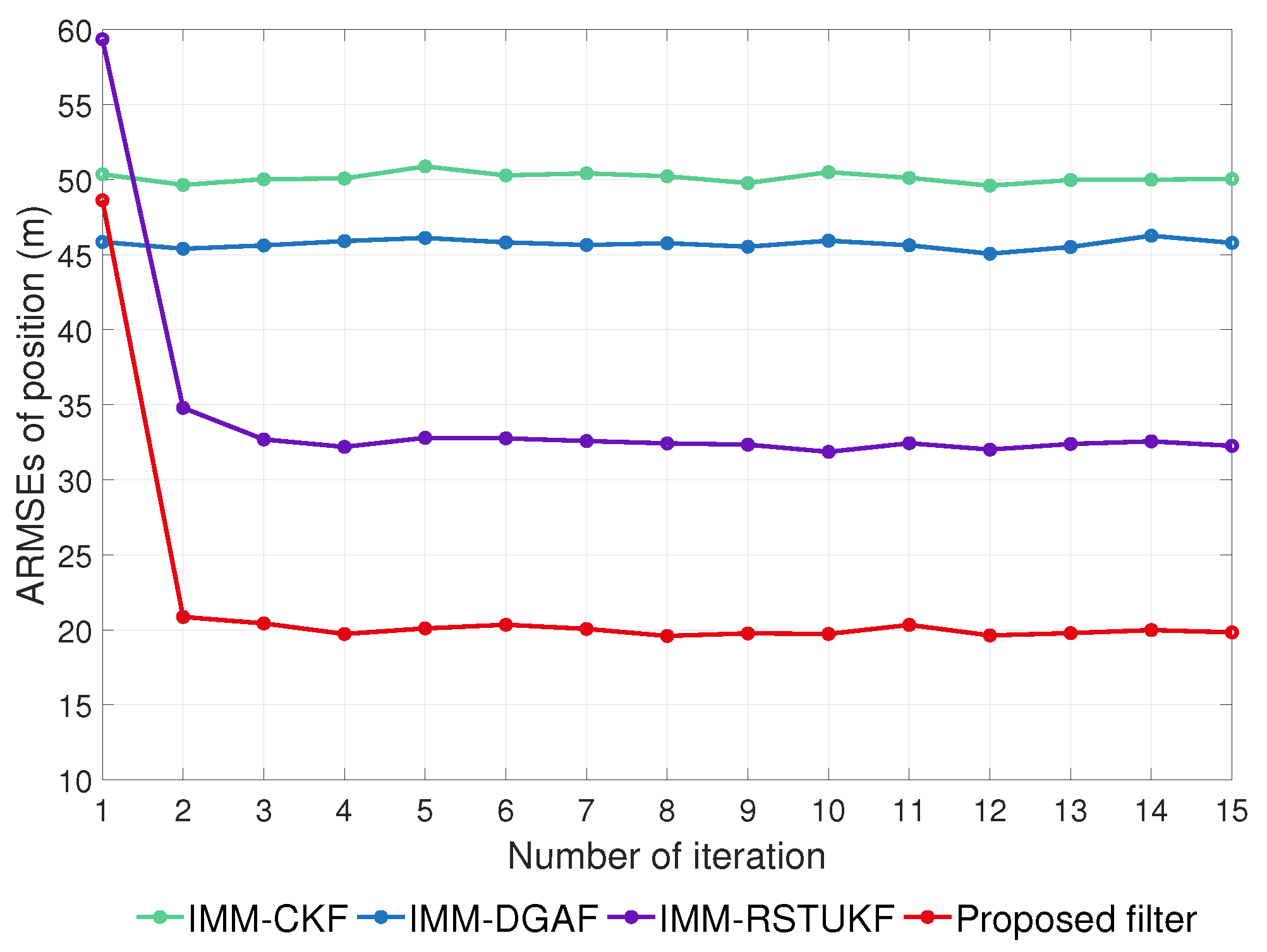
ARMSE${}_{pos}$  (m)	1∼200	37.28	24.42	27.69	12.77
	201∼400	53.33	35.49	52.29	21.60
	401∼600	47.07	28.45	37.60	15.66
	601∼800	65.01	41.03	61.88	26.29
	801∼1000	48.90	29.13	39.99	16.47
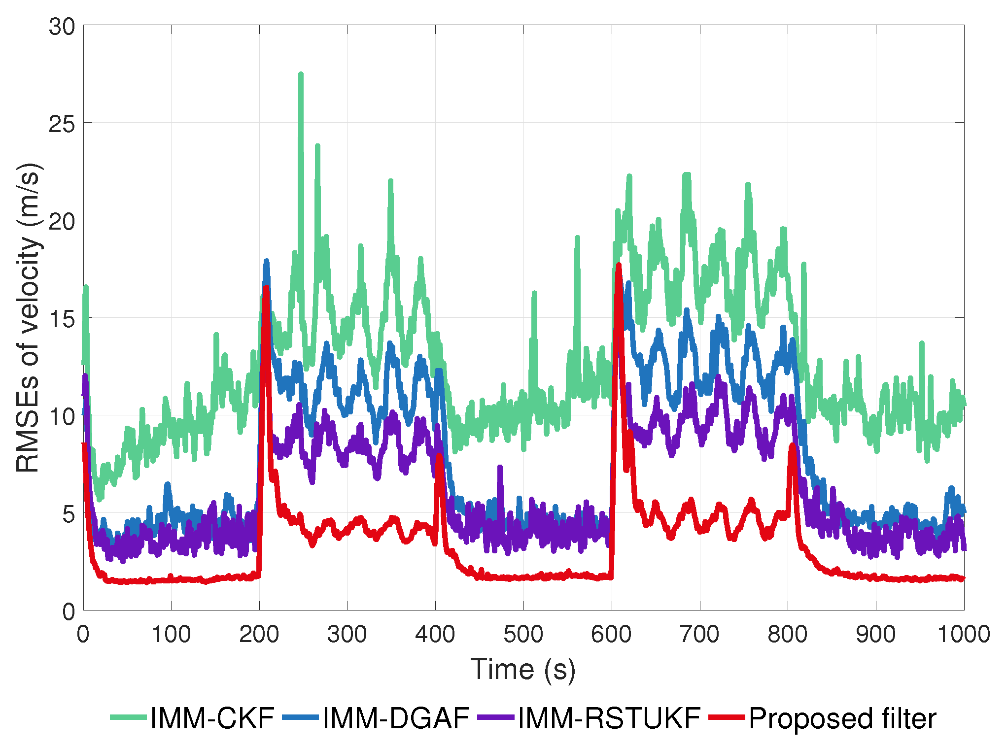
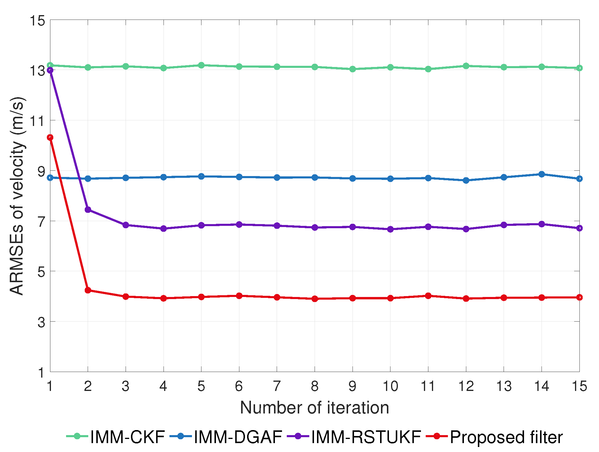
ARMSE${}_{vel}$  (m/s)	1∼200	10.45	3.87	4.55	1.75
	201∼400	16.00	8.79	11.64	4.74
	401∼600	11.65	4.37	5.28	2.06
	601∼800	18.06	9.52	12.48	5.41
	801∼1000	19.84	4.39	5.51	2.14
ARMSE${}_{omg}$  (deg/s)	1∼200	3.33	1.12	1.10	0.77
	201∼400	9.80	9.07	9.08	8.85
	401∼600	3.19	1.30	1.27	0.91
	601∼800	9.73	8.91	8.94	8.71
	801∼1000	6.23	1.28	1.33	0.94
SSIT (ms)	1∼1000	0.166	1.632	0.264	1.651

shows that the designed filter has smaller ARMSEs in each period in the scenarios of HTMNs coexisting with OSRMD. Compared with IMM-RSTUKF, which utilizes VB approach, the accuracy of ARMSE in position, velocity and turning rate of the designed filter is improved by $41.46\%$, $47.96\%$ and $6.92\%$, respectively. Moreover, the introduction of the VB inference increases computational costs.

The second experiment part validates the impact of different OSRMD probabilities on estimation accuracy. The range of the measurement delay probability ${\phi }_s$ is set to be from $0.1$ to $0.9$. In Figure 6, Figure 7 and Figure 8, the ARMSEs of the positions, velocities, and turning rate from the designed filtering method and existing algorithms are provided. The horizontal axises of Figure 6, Figure 7 and Figure 8 denote different measurement delay probabilities, and the longitudinal axises of Figure 6, Figure 7 and Figure 8 represent the value of ARMSEs. From Figure 6, Figure 7 and Figure 8, it can be seen that the IMM-CKF shows the worst estimation performance among all filters. The reason is that IMM-CKF deals with neither measurement outliers nor random measurement delay, leading to unsatisfactory estimation performance. As the probability of delay increases, the ARMSEs of IMM-RSTUKF has a relatively large change, the reason is that the IMM-RSTUKF lacks of adaptive estimation ability to random measurement delay. For the IMM-DGAF, although it has good adaptability to random measurement delay, it still has large estimation error due to inaccurate modeling of HTMNs. Since the proposed method can address the HTMNs and OSRMD simultaneously, this algorithm shows better adaptability to different measurement delays and obtain higher estimation accuracy in the presence of measurement outliers than existing algorithms.

The third part of the experiment aimed to verify the performances of all filters under different measurement outlier probabilities. The fixed measurement outlier probability value in Equation (69) is transformed into a range from $0.05$ to $0.15$. Figure 9, Figure 10 and Figure 11 exhibits the ARMSEs from all algorithms under different measurement outlier probabilities. It can be seen from Figure 9, Figure 10 and Figure 11 that the IMM-CKF still performs poorly, the conclusions about the IMM-CKF in the second experiment are further verified. In addition, with the increasing of the measurement outlier probability, the ARMSE value of the IMM-DGAF shows great fluctuation, this is because the IMM-DGAF assumes the measurement noises to obey Gaussian distributions, however, the Gaussian distribution is sensitive to outliers. As a result, the IMM-DGAF shows serious performance degradation to the increase of the measurement outlier probability. The reason for the IMM-RSTUKF performs worse than the proposed method is that the IMM-RSTUKF assumes all the measurement vectors can arrive in time, which is not satisfied when the OSRMD exists. The results in Figure 9, Figure 10 and Figure 11 indicate that the presented algorithm can achieve better adaptive estimation performances than existing algorithms under different measurement outlier probabilities.

In the fourth part of the experiment, the effects of the variational iterations on filtering accuracy are validated individually. In Figure 12, Figure 13 and Figure 14, the ARMSEs from all filters under different variational iterations $N=1$, 2, …, 15 are shown. The simulation results in Figure 12, Figure 13 and Figure 14 indicate that the presented algorithm converges when iteration number $N=2$, and performs better than existing filters in estimation accuracy when $N\ge 2$. The proposed algorithm converges faster than the IMM-RSTUKF which is also based on the VB framework. We can see from Figure 12, Figure 13 and Figure 14 that the estimation accuracy of the IMM-CKF and IMM-DGAF is relatively stable since these two algorithms do not depend on the variational iterations. As the variational iteration N increases, the estimation performance of the designed filter improves. However, computational efficiency must be taken into account. Considering the balance between computing efficiency and estimation performances, the recommended variational iteration number is 4 to 8.

6. Conclusions

In the applications of surface maneuvering target tracking, due to the adverse effects of unreliable sensors and communication channel latency, the measurement outliers and random measurement delay often occur simultaneously. The state estimation issue of surface maneuver target faces severe challenges. Aiming at solving the problem of state estimation in JMSs with HTMNs and OSRMD, this paper designed a novel robust IMM filtering method and applied to surface maneuvering target tracking. Firstly, the HTMNs are assumed to follow STDs, and we introduced an RBV to characterize the random measurement delay. Secondly, this paper established a new HGSSM to utilize VB method. Finally, by using VB inference, the system state, RBV, and model probability are estimated simultaneously. The surface maneuvering target tracking simulation results indicated that the designed filtering method has better estimation accuracy than existing algorithms. In addition, compared with existing filters, the proposed filtering method showed better robustness to different outlier probabilities, and achieved better adaptive estimation performances under various of random measurement delay probabilities. Although the computational costs of the designed method increased slightly, the accuracy of ARMSE in position, velocity and turning rate is improved by $41.46\%$, $47.96\%$ and $6.92\%$ than the state-of-the-art, respectively. In our future work, based on the theoretical content and results of the proposed filtering method, more complex measurement environments will be considered, including the cases of multi-step random measurement delay and random measurement loss with unknown probability. The effect of heavy-tailed process noises on filtering accuracy and computational efficiency are also focuses of our future research.

References

- Zhang, W.; Zhao, X.; Liu, Z.; Liu, K.; Chen, B. Converted state equation Kalman filter for nonlinear maneuvering target tracking. Signal Process. 2023, 202, 108741. [Google Scholar] [CrossRef]
- Huang, Y.; Zhang, Y.; Zhao, Y.; Shi, P.; Chambers, J.A. A novel outlier-robust Kalman filtering framework based on statistical similarity measure. IEEE Trans. Autom. Control 2020, 66, 2677–2692. [Google Scholar] [CrossRef]
- Xu, B.; Hu, J.; Guo, Y. An Acoustic Ranging Measurement Aided SINS/DVL Integrated Navigation Algorithm Based on Multivehicle Cooperative Correction. IEEE Trans. Instrum. Meas. 2022, 71, 1–15. [Google Scholar] [CrossRef]
- Demirci, M.; Gözde, H.; Taplamacioglu, M.C. Improvement of power transformer fault diagnosis by using sequential Kalman filter sensor fusion. Int. J. Electr. Power Energy Syst. 2023, 149, 109038. [Google Scholar] [CrossRef]
- Lindner, L.; Sergiyenko, O.; Rivas-López, M.; Ivanov, M.; Rodríguez-Quiñonez, J.C.; Hernández-Balbuena, D.; Flores-Fuentes, W.; Tyrsa, V.; Muerrieta-Rico, F.N.; Mercorelli, P. Machine vision system errors for unmanned aerial vehicle navigation. In Proceedings of the 2017 IEEE 26th International Symposium on Industrial Electronics (ISIE), Edinburgh, UK, 19–21 June 2017; pp. 1615–1620. [Google Scholar]
- Mercorelli, P.; Lehmann, K.; Liu, S. Robust flatness based control of an electromagnetic linear actuator using adaptive PID controller. In Proceedings of the 42nd IEEE International Conference on Decision and Control (IEEE Cat. No. 03CH37475), Maui, HI, USA, 9–12 December 2003; Volume 4, pp. 3790–3795. [Google Scholar]
- Li, K.; Zhao, S.; Liu, F. Joint state estimation for nonlinear state-space model with unknown time-variant noise statistics. Int. J. Adapt. Control Signal Process. 2021, 35, 498–512. [Google Scholar] [CrossRef]
- Li, X.R.; Jilkov, V.P. Survey of maneuvering target tracking. Part V. Multiple-model methods. IEEE Trans. Aerosp. Electron. Syst. 2005, 41, 1255–1321. [Google Scholar]
- Freni, G.; Mannina, G.; Viviani, G. Urban runoff modelling uncertainty: Comparison among Bayesian and pseudo-Bayesian methods. Environ. Model. Softw. 2009, 24, 1100–1111. [Google Scholar] [CrossRef]
- Djuric, P.M.; Kotecha, J.H.; Zhang, J.; Huang, Y.; Ghirmai, T.; Bugallo, M.F.; Miguez, J. Particle filtering. IEEE Signal Process. Mag. 2003, 20, 19–38. [Google Scholar] [CrossRef]
- Seah, C.E.; Hwang, I. Algorithm for performance analysis of the IMM algorithm. IEEE Trans. Aerosp. Electron. Syst. 2011, 47, 1114–1124. [Google Scholar] [CrossRef]
- Hwang, I.; Seah, C.E.; Lee, S. A study on stability of the interacting multiple model algorithm. IEEE Trans. Autom. Control 2016, 62, 901–906. [Google Scholar] [CrossRef]
- Zhao, S.; Ahn, C.; Shi, P.; Shmaliy, Y.; Liu, F. Bayesian State Estimations for Markovian Jump Systems: Employing Recursive Steps and Pseudocodes. IEEE Syst. Man, Cybern. Mag. 2019, 5, 27–36. [Google Scholar] [CrossRef]
- Li, J.; Yuan, G.; Duan, H. Consensus CIF-Based IMM Filtering for Multiple-UAV Target Tracking. In Proceedings of the 2022 International Conference on Guidance, Navigation and Control: Advances in Guidance, Navigation and Control, Tianjin, China, 23–25 October 2020; pp. 7060–7069. [Google Scholar]
- Youn, W.; Ko, N.Y.; Gadsden, S.A.; Myung, H. A novel multiple-model adaptive Kalman filter for an unknown measurement loss probability. IEEE Trans. Instrum. Meas. 2020, 70, 1–11. [Google Scholar] [CrossRef]
- Zubača, J.; Stolz, M.; Seeber, R.; Schratter, M.; Watzenig, D. Innovative Interaction Approach in IMM Filtering for Vehicle Motion Models With Unequal States Dimension. IEEE Trans. Veh. Technol. 2022, 71, 3579–3594. [Google Scholar] [CrossRef]
- Blair, W.D.; Watson, G. Interacting multiple bias model algorithm with application to tracking maneuvering targets. In Proceedings of the 1992 31st IEEE Conference on Decision and Control, Tucson, AZ, USA, 16–18 December 1992; pp. 3790–3795. [Google Scholar]
- Sarkka, S.; Nummenmaa, A. Recursive noise adaptive Kalman filtering by variational Bayesian approximations. IEEE Trans. Autom. Control 2009, 54, 596–600. [Google Scholar] [CrossRef]
- Huang, Y.; Zhang, Y.; Wu, Z.; Li, N.; Chambers, J. A novel adaptive Kalman filter with inaccurate process and measurement noise covariance matrices. IEEE Trans. Autom. Control 2017, 63, 594–601. [Google Scholar] [CrossRef]
- Huang, Y.; Zhang, Y.; Li, N.; Wu, Z.; Chambers, J.A. A novel robust Student’s t-based Kalman filter. IEEE Trans. Aerosp. Electron. Syst. 2017, 53, 1545–1554. [Google Scholar] [CrossRef]
- Zhu, H.; Zhang, G.; Li, Y.; Leung, H. An adaptive Kalman filter with inaccurate noise covariances in the presence of outliers. IEEE Trans. Autom. Control 2021, 67, 374–381. [Google Scholar] [CrossRef]
- Jia, G.; Huang, Y.; Zhang, Y.; Chambers, J. A novel adaptive Kalman filter with unknown probability of measurement loss. IEEE Signal Process. Lett. 2019, 26, 1862–1866. [Google Scholar] [CrossRef]
- Wang, G.; Wang, X.; Zhang, Y. Variational Bayesian IMM-filter for JMSs with unknown noise covariances. IEEE Trans. Aerosp. Electron. Syst. 2019, 56, 1652–1661. [Google Scholar] [CrossRef]
- Shen, C.; Xu, D.; Huang, W.; Shen, F. An interacting multiple model approach for state estimation with non-Gaussian noise using a variational Bayesian method. Asian J. Control 2015, 17, 1424–1434. [Google Scholar] [CrossRef]
- Li, D.; Sun, J. Robust Interacting Multiple Model Filter Based on Student’st-Distribution for Heavy-Tailed Measurement Noises. Sensors 2019, 19, 4830. [Google Scholar] [CrossRef] [PubMed]
- Yan, B.; Zuo, J.; Chen, X.; Zou, H. Improved multiple model particle filter for maneuvering target tracking in the presence of delayed measurements. In Proceedings of the 2017 International Conference on Computer Systems, Electronics and Control (ICCSEC), Dalian, China, 25–27 December 2017; pp. 810–814. [Google Scholar]
- Wang, X.; Liang, Y.; Pan, Q.; Zhao, C. Gaussian filter for nonlinear systems with one-step randomly delayed measurements. Automatica 2013, 49, 976–986. [Google Scholar] [CrossRef]
- Tong, Y.; Zheng, Z.; Fan, W.; Li, Q.; Liu, Z. An improved unscented Kalman filter for nonlinear systems with one-step randomly delayed measurement and unknown latency probability. Digit. Signal Process. 2022, 121, 103324. [Google Scholar] [CrossRef]
- Ito, K.; Xiong, K. Gaussian filters for nonlinear filtering problems. IEEE Trans. Autom. Control 2000, 45, 910–927. [Google Scholar] [CrossRef]
- Bai, M.; Huang, Y.; Chen, B.; Yang, L.; Zhang, Y. A novel mixture distributions-based robust Kalman filter for cooperative localization. IEEE Sens. J. 2020, 20, 14994–15006. [Google Scholar] [CrossRef]
- Huang, Y.; Zhang, Y.; Zhao, Y.; Chambers, J.A. A novel robust Gaussian–Student’s t mixture distribution based Kalman filter. IEEE Trans. Signal Process. 2019, 67, 3606–3620. [Google Scholar] [CrossRef]
- Huang, Y.; Zhang, Y.; Chambers, J.A. A novel Kullback–Leibler divergence minimization-based adaptive student’s t-filter. IEEE Trans. Signal Process. 2019, 67, 5417–5432. [Google Scholar] [CrossRef]
- Lu, C.; Feng, W.; Li, W.; Zhang, Y.; Guo, Y. An adaptive IMM filter for jump Markov systems with inaccurate noise covariances in the presence of missing measurements. Digit. Signal Process. 2022, 127, 103529. [Google Scholar] [CrossRef]
- Roth, M.; Özkan, E.; Gustafsson, F. A Student’s t filter for heavy tailed process and measurement noise. In Proceedings of the 2013 IEEE International Conference on Acoustics, Speech and Signal Processing, Vancouver, BC, Canada, 26–31 May 2013; pp. 5770–5774. [Google Scholar]
- Jia, G.; Huang, Y.; Bai, M.B.; Zhang, Y. A novel robust Kalman filter with non-stationary heavy-tailed measurement noise. IFAC-PapersOnLine 2020, 53, 368–373. [Google Scholar] [CrossRef]
- Fu, H.; Cheng, Y. A Novel Robust Kalman Filter Based on Switching Gaussian-Heavy-Tailed Distribution. IEEE Trans. Circuits Syst. II Express Briefs 2022, 69, 3012–3016. [Google Scholar] [CrossRef]