Article

Three-Dimensional Trajectory Tracking of AUV Based on Nonsingular Terminal Sliding Mode and Active Disturbance Rejection Decoupling Control

College of Intelligent Systems Science and Engineering, Harbin Engineering University, Harbin 150001, China
*
Author to whom correspondence should be addressed.
J. Mar. Sci. Eng. 2023, 11(5), 959; https://doi.org/10.3390/jmse11050959
Submission received: 24 March 2023 / Revised: 24 April 2023 / Accepted: 26 April 2023 / Published: 30 April 2023
(This article belongs to the Special Issue Motion Control and Path Planning of Marine Vehicles)

Abstract

:
This paper presents a nonsingular terminal sliding mode and active disturbance rejection decoupling control (NTSM-ADRDC) scheme for the three-dimensional (3D) trajectory tracking of autonomous underwater vehicles (AUV). Firstly, the AUV model is decoupled into five independent single input–single output (SISO) channels using ADRDC technology. Secondly, the NTSM-ADRDC controller is designed. The linear extended state observer (LESO) is used to observe the AUV state variables, and estimate the total disturbance of the system. In addition, to improve the system error convergence rate, the combination of exponential reaching rate and NTSM constitutes a nonlinear states error feedback control law for the controller. Finally, the stability of the proposed control law is proved using the Lyapunov theory. The simulation results demonstrate the effectiveness and robustness of the designed NTSM-ADRDC trajectory tracking approach.

1. Introduction

Autonomous underwater vehicles (AUV) are increasingly being utilized in a variety of civil and military applications, such as intelligence collection, ocean mapping, pipeline inspection, and maritime rescue [1,2]. In order to better perform these tasks, it is essential that the AUV has the ability to accurately track three-dimensional (3D) trajectories in underwater space [3]. However, due to the highly nonlinear, strong coupling, complex hydrodynamic coefficient of the AUV model, the precise control of AUV has become a significant challenge [4]. Moreover, the sensitivity of AUVs to external disturbances further increases the difficulty in controller design [5]. Therefore, how to design an AUV trajectory tracking controller with good robustness has become a research hotspot.
The trajectory tracking of AUVs has been the subject of extensive research in recent years, and various control methods have been used in the design of AUV controllers. These control methods mainly include proportional–integral–derivative (PID) control [6,7], fuzzy logic control [8,9], adaptive control [10,11], neural network control (NNC) [12,13], and model predictive control [14,15,16]. In the literature [6], an intelligent PID controller is applied to AUV’s horizontal plane path tracking control and vertical plane depth control. However, PID cannot provide accurate control in the presence of ocean current disturbances. In [8], a fuzzy dynamic surface control method was designed for solving the 3D trajectory tracking problem of the under-actuated AUV in the presence of model uncertainty and time-varying disturbance. To solve the dynamic trajectory tracking control of AUV in a three-dimensional underwater environment, a variable fuzzy predictor-based predictive control approach was proposed [9]. However, the membership functions and fuzzy rules of fuzzy logic control need to be determined based on rich experience. An adaptive controller based on Lyapunov’s direct method and the back-stepping technique was proposed [10], which can address the issue of trajectory tracking control of underactuated AUV of six degrees of freedom. In the literature [11], an adaptive disturbance observer has been designed for AUV trajectory tracking control in the presence of unknown external disturbances, and the gain of the observer can be adjusted automatically by introducing an adaptive law. However, adaptive control can only achieve good control effects if the model of the controlled object is known, the parameters change slowly, and the uncertainty of the system is finite. A neural network-based tracking control method for underactuated AUV with model uncertainties was presented [12]. Simulation results demonstrated the effectiveness of the proposed control strategy. However, due to a large amount of calculation, NNC cannot meet the real-time requirement of AUV. The literature [14] presented a novel 3D underwater trajectory tracking approach for underwater robots based on model predictive control, considering actual constraints on system inputs and states. The main disadvantage of MPC is that it not only relies on an accurate mathematical model but also requires a high level of computational power of the AUV. Although the above control algorithm has achieved a better trajectory tracking effect to a certain extent, there are still some respective weaknesses.
The active disturbance rejection control (ADRC) algorithm can effectively solve the problem of system uncertainty (internal model and external disturbance uncertainty) [17,18]. The unique anti-interference capability of ADRC technology allows for a wide range of applications in engineering control fields [19,20]. ADRC was first proposed by Han in the 1990s [21,22]. As the core of ADRC, the extended state observer (ESO) can estimate the total disturbance including internal dynamics and external disturbance. Furthermore, the nonlinear states error feedback control law can compensate for the total disturbance of the system [23]. The control objective of the ADRC is to converge the system state error to zero so that the desired control effect can be achieved. However, the traditional ADRC has too many parameters, so it is difficult to set the parameters in engineering applications. To simplify the structure of ADRC, Professor Gao designed a linear active disturbance rejection controller (LADRC) [24]. The LADRC simplified the control parameters compared to ADRC, which is very convenient for engineering applications. In addition, the theory for the stability proof of LDARC was provided by Gao [25].
Sliding mode variable structure control has received extensive attention from scholars due to its ideal robustness [26,27]. For example, a second-order sliding mode controller is designed to addresses the problems of depth regulation control of AUV in wave circumstance [28].The simulation results show that this method can be effectively applied to robust tracking of AUV. However, chattering is the main drawback of sliding mode control. The literature [29] proposed a non-singular terminal sliding mode control (NTSMC) method, which can effectively suppress chattering and avoid singular. In the literature [30], an NTSMC method based on an exponential convergence law was proposed to improve the convergence speed for reaching non-singular terminal sliding surfaces. The simulation results showed that the designed control law can make the system converge to the equilibrium point in a short time.
In order to solve the problem of external disturbances and ocean current in AUV 3D trajectory tracking control, and also include the problem of tracking error convergence. A novel control scheme based on NTSM-ADRDC is proposed in this paper. The main idea is to combine the strong robustness of the NTSMC method with the LADRC controller’s ability to suppress model uncertainty and external disturbance. Firstly, the AUV model is decoupled by taking advantage of active disturbance rejection decoupling control technology, in which a new virtual control vector is introduced. Then, the LESO is utilized to estimate the internal unmodeled dynamics and external disturbance of the AUV system as the total disturbance. After that, the NTSM nonlinear states error feedback control law is designed to compensate for the total disturbance of the system. Finally, the stability of the AUV system is proved by the Lyapunov theory.
The rest of this paper is organized as follows: the AUV model and its decoupling control process are given in Section 2. Section 3 illustrates the total structure of the AUV trajectory tracking control based on NTSM-ADRDC and the detailed proof of the controller’s stability. Section 4 verifies the effectiveness of the designed controller through simulation. Finally, the conclusions are given in Section 5.

2. AUV Model and Decoupling

In this section, the kinematics and dynamics model of the AUV is first described. Then, the decoupling control of the AUV model based on the ADRC technique is introduced.

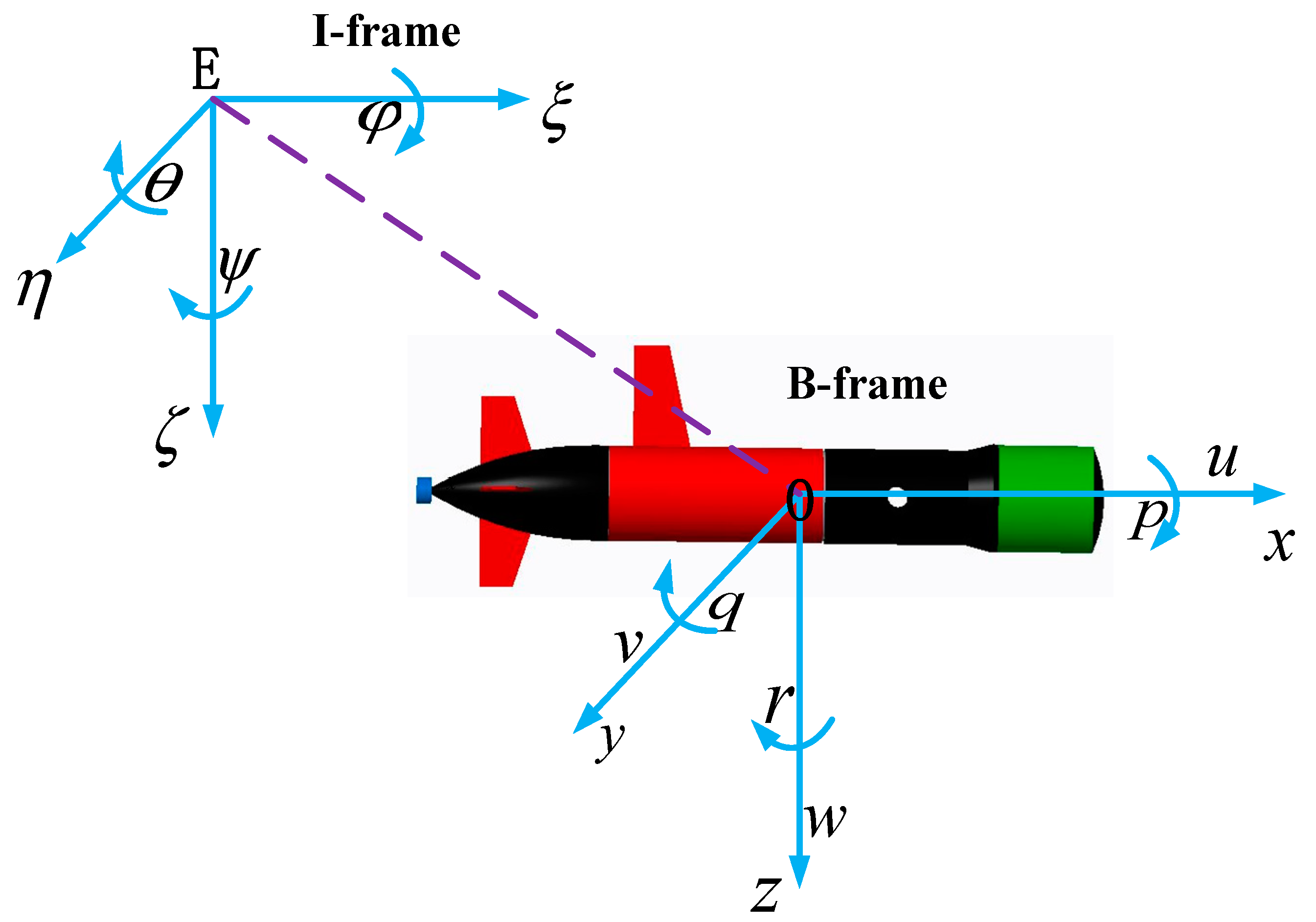
2.1. AUV Kinematics and Dynamics

Establishing the kinematics and dynamics model of the AUV is the prerequisite for studying its motion control. The inertial reference frame (I-frame) and body-fixed frame (B-frame) of the AUV are depicted in Figure 1. We assumed the rol1 of the AUV is passively stable, and its coupling nonlinear effect can be ignored. Based on the assumption, the kinematic and dynamic model of a five-degrees-of-freedom (5-DOF) full actuated AUV are stated as follows [31]:
{ x ˙ = u cos ψ cos θ v sin ψ + w sin θ cos ψ y ˙ = u sin ψ cos θ + v cos ψ + w sin θ sin ψ z ˙ = u sin θ + w cos θ θ ˙ = q ψ ˙ = r / cos θ
{ u ˙ = m 22 m 11 v r m 33 m 11 w q d 11 m 11 u + 1 m 11 τ u + 1 m 11 d u v ˙ = m 11 m 22 u r d 22 m 22 v + 1 m 22 τ v w ˙ = m 11 m 33 u q d 33 m 33 w + 1 m 33 τ w + 1 m 33 d w q ˙ = m 33 m 11 m 55 u w d 55 m 55 q + 1 m 55 τ q + 1 m 55 d q r ˙ = m 11 m 22 m 66 u v d 66 m 66 r + 1 m 66 τ r + 1 m 66 d r
where η = [ η 1 η 2 ] T represent the position and Euler angles of the AUV in I-frame. η 1 = [ x y z ] T indicate the north, east, and depth coordinates of the AUV. η 2 = [ θ ψ ] T indicate the pitch and yaw angle of the AUV. v = [ v 1 v 2 ] T represent the linear velocity and angular velocity of the AUV in B-frame. v 1 = [ u v w ] T denote the longitudinal, lateral, and vertical velocity of the AUV. v 2 = [ q r ] T denote the pitch and yaw angular velocity of the AUV. τ = [ τ 1 τ 2 ] T are the input forces and moments of the AUV system. τ 1 = [ τ u τ v τ w ] T are the longitudinal, lateral, and vertical input forces. τ 2 = [ τ q τ r ] T are the pitch and yaw input moments. m i i , d j j represent AUV hydrodynamic parameters and damping coefficients, m 11 = m X u ˙ ,   m 22 = m Y v ˙ ,   m 33 = m Z w ˙ ,   m 55 = I y M q ˙ ,   m 66 = I z N r ˙ , d 11 = X u X u | u | | u | , d 22 = Y v Y v | v | | v | ,   d 33 = Z w Z w | w | | w | ,   d 55 = M q M q | q | | q | . d = [ d u d v d w d q d r ] T represent bounded external disturbances. For detailed definitions of hydrodynamic parameters of AUV, readers can refer to the literature [32,33].

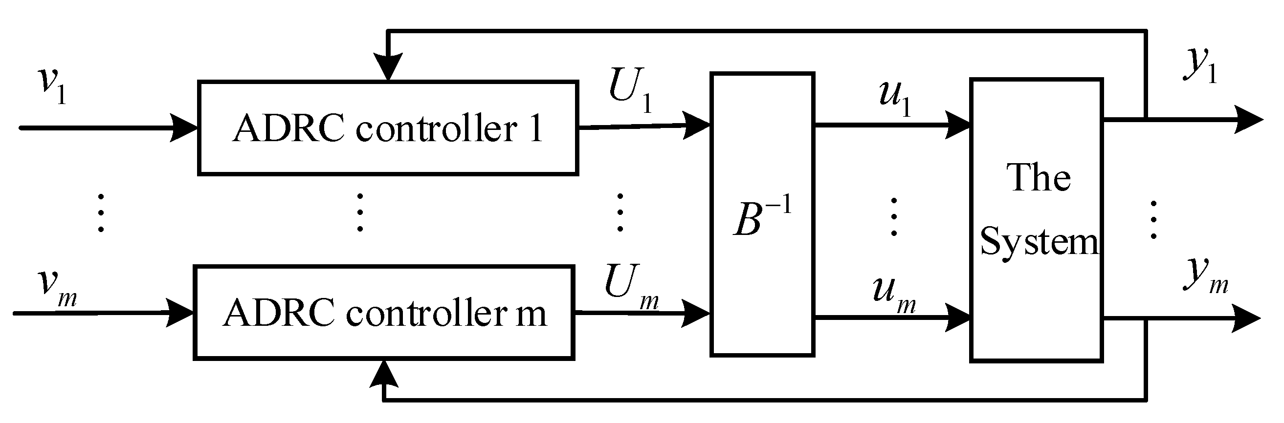
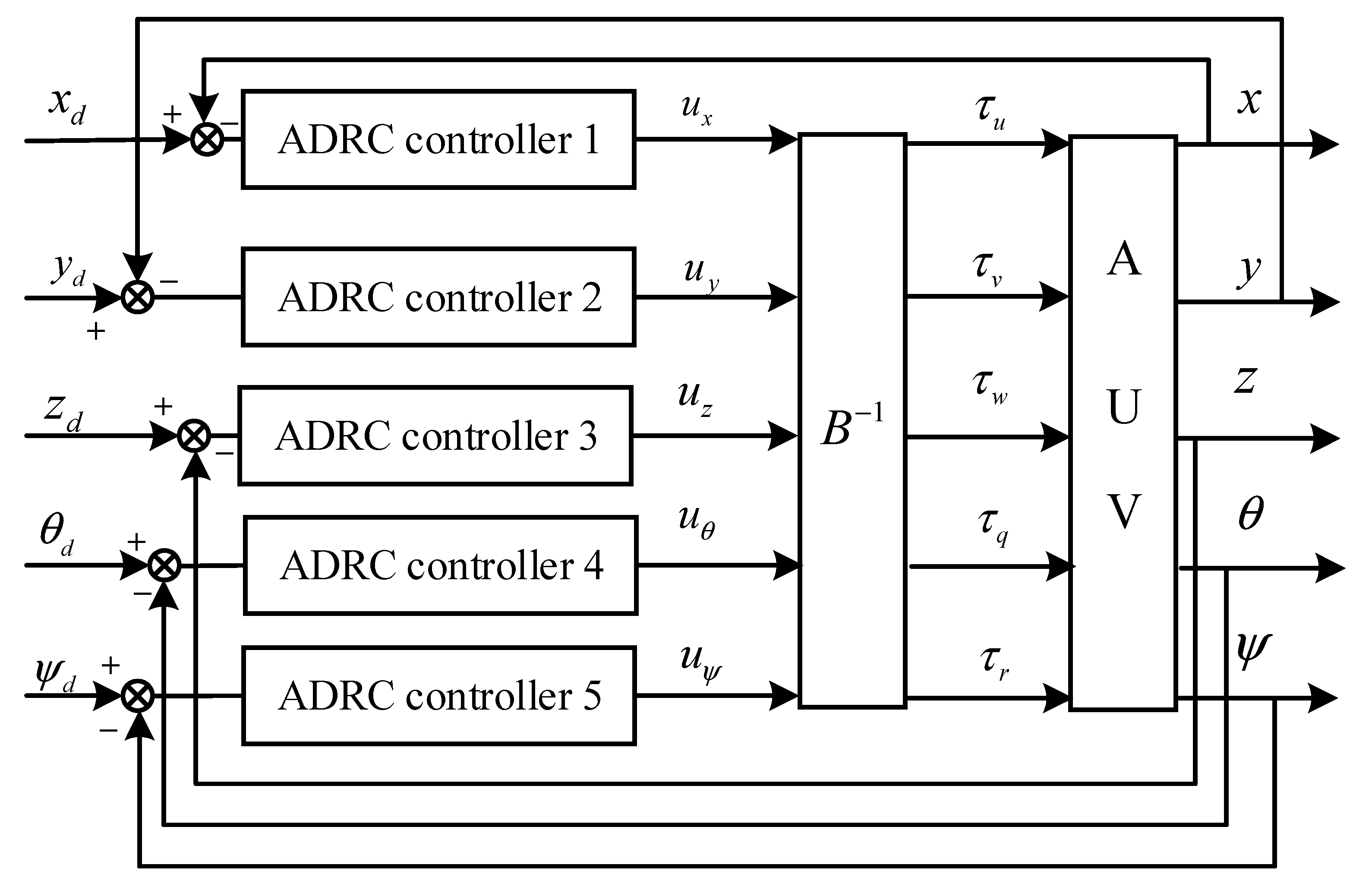
2.2. Decoupling Control of AUV Model

From the above-established AUV multi-input and multi-output (MIMO) system, we can observe that the AUV is a nonlinear, multivariable, strongly coupled system. It brings a dramatic challenge to the subsequent design of the AUV tracking controller due to its characteristics. The ADRC technique is a good scheme for solving control problems of the coupled MIMO system. When using the ADRC technique for decoupling control of MIMO system, the coupling term between the different input and output channels can be seen as an external disturbance. The ADRC controller for each channel can estimate and compensate for external disturbances independently, thus achieving the decoupling of control for each channel by introducing virtual control variables. Next, the active disturbance rejection decoupling control technology will be introduced in detail [34].
Suppose there is an m-dimensional MIMO system as follows:
{ x ¨ 1 = f 1 ( x 1 , x ˙ 1 , , x m , x ˙ m ) + b 11 u 1 + + b 1 m u m x ¨ 2 = f 2 ( x 1 , x ˙ 1 , , x m , x ˙ m ) + b 21 u 1 + + b 2 m u m x ¨ m = f m ( x 1 , x ˙ 1 , , x m , x ˙ m ) + b m 1 u 1 + + b m m u m y 1 = x 1 , y 2 = x 2 , , y m = x m
where x i , y i ( i = 1 , 2 m ) are, respectively, expressed as system state variables and output; u i represents control input; the amplification factor of the control variable b i j = b i j ( x , x ˙ , t ) is a function of state variables and time, which can be written in a matrix form as:
B ( x , x ˙ , t ) = [ b 11 ( x , x ˙ , t ) b 1 m ( x , x ˙ , t ) b m 1 ( x , x ˙ , t ) b m m ( x , x ˙ , t ) ]
If the control variable coefficient matrix B ( x , x ˙ , t ) is invertible, the system Equation (3) can be simplified as:
{ x ¨ = f ( x , x ˙ , t ) + U y = x
where x = [ x 1 x 2 x m ] T , y = [ y 1 y 2 y m ] T , f = [ f 1 f 2 f m ] T , u = [ u 1 u 2 u m ] T , U = B ( x , x ˙ , t ) u is the newly introduced virtual control vector.
Therefore, the i - t h channel in the system (5) can be expressed as:
{ x ¨ i = f i ( x 1 , x ˙ 1 , , x m , x ˙ m , t ) + U i y i = x i
Essentially, the ADRC technology regards the f i ( x 1 , x ˙ 1 , , x m , x ˙ m , t ) of i-th channel as the external disturbance of the channel, while the ADRC controller of each channel can estimate and compensate for the external disturbance independently. Therefore, the virtual control variable Ui and the output variable y i of each channel are in SISO relationship, that is, the system realizes the complete decoupling control by introducing virtual control vector. The decoupling control process of the MIMO system based on active disturbance rejection technology is shown in Figure 2. The desired input value v i ( i = 1 , 2 m ) and the actual output value y i ( i = 1 , 2 m ) of the system constitute a closed-loop channel. Each ADRC controller can achieve independent control of the corresponding channel so that the actual output of the system converges to the desired value.
For the 5-DOF model of AUV in Equations (1) and (2), which is a strongly coupled MIMO system. In order to facilitate the design of the controller in the latter, it is necessary to decouple the control of the AUV model using the ADRC technique.
First, the derivation of Equation (1) is obtained:
{ x ¨ = u ˙ cos θ cos ψ u cos θ sin ψ ψ ˙ u sin θ cos ψ θ ˙ v ˙ sin ψ             v cos ψ ψ ˙ + w ˙ sin θ cos ψ + w cos θ cos ψ θ ˙ w sin θ sin ψ ψ ˙ y ¨ = u ˙ cos θ sin ψ u sin θ sin ψ θ ˙ + u cos θ cos ψ ψ ˙ + v ˙ cos ψ             v sin ψ ψ ˙ + w ˙ sin θ cos ψ + w cos θ sin ψ θ ˙ + w sin θ cos ψ ψ ˙ z ¨ = u ˙ sin θ u cos θ θ ˙ + w ˙ cos θ w sin θ θ ˙ θ ¨ = q ˙ ψ ¨ = r ˙ sec θ + r tan θ sec θ
Next, substitute Equation (2) into Equation (7):
{ x ¨ = f 1 ( u , v , w , q , r , θ , ψ ) + 1 m 11 cos ψ cos θ ( τ u + d u ) 1 m 22 sin ψ ( τ v + d v ) + 1 m 33 cos ψ sin θ ( τ w + d w ) y ¨ = f 2 ( u , v , w , q , r , θ , ψ ) + 1 m 11 sin ψ cos θ ( τ u + d u ) + 1 m 22 sin ψ ( τ v + d v ) + 1 m 33 sin ψ sin θ ( τ w + d w ) z ¨ = f 3 ( u , v , w , q , r , θ ) 1 m 11 sin θ ( τ u + d u ) + 1 m 33 cos θ ( τ w + d w ) θ ¨ = f 4 ( u , w , q ) + 1 m 55 ( τ q + d q ) ψ ¨ = f 5 ( u , v , r , θ ) + 1 m 66 sec θ ( τ r + d r )
where f i ( i = 1 , 2 , 3 , 4 , 5 ) is the sum of other items except τ and d .
Here, we will introduce a new virtual control vector as follows:
U = B * τ
With
U = [ u x u y u z u θ u ψ ] T
B = [ cos ψ cos θ m 11 sin ψ m 22 cos ψ sin θ m 33 0 0 sin ψ cos θ m 11 cos ψ m 22 sin ψ sin θ m 33 0 0 sin θ m 11 0 cos θ m 33 0 0 0 0 0 1 m 55 0 0 0 0 0 sec θ m 66 ]
After calculation, | B | = sec θ / m 11 m 22 m 33 m 55 m 66 is reversible, the Equation (8) can be simplified as:
{ x ¨ = f 1 ( u , v , w , q , r , θ , ψ ) + w 1 + u x y ¨ = f 2 ( u , v , w , q , r , θ , ψ ) + w 2 + u y z ¨ = f 3 ( u , v , w , q , r , θ ) + w 3 + u z θ ¨ = f 4 ( u , w , q ) + w 4 + u q ψ ¨ = f 5 ( u , v , r , θ ) + w 5 + u r
where w = [ w 1 w 2 w 3 w 4 w 5 ] T , w = B * d .
The decoupling control process of the AUV system based on ADRC technology is shown in Figure 3. The ADRC technology regards f i + w i ( i = 1 , 2 , 3 , 4 , 5 ) as the total external disturbance of the i-th channel of the AUV system, while the ADRC controller of each channel can estimate and compensate for the total disturbance independently. Therefore, the virtual control variable U and the output variable η of each channel are in SISO relationship, that is, the AUV system realizes the complete decoupling control through virtual control vector U . The five channels of the AUV system can be individually designed with controllers. η d = [ x d y d z d θ d ψ d ] T are the reference signals of position and angle of AUV. Through the action of the control coefficient matrix B−1, the virtual control vector U can generate the real control input τ acting on the AUV.

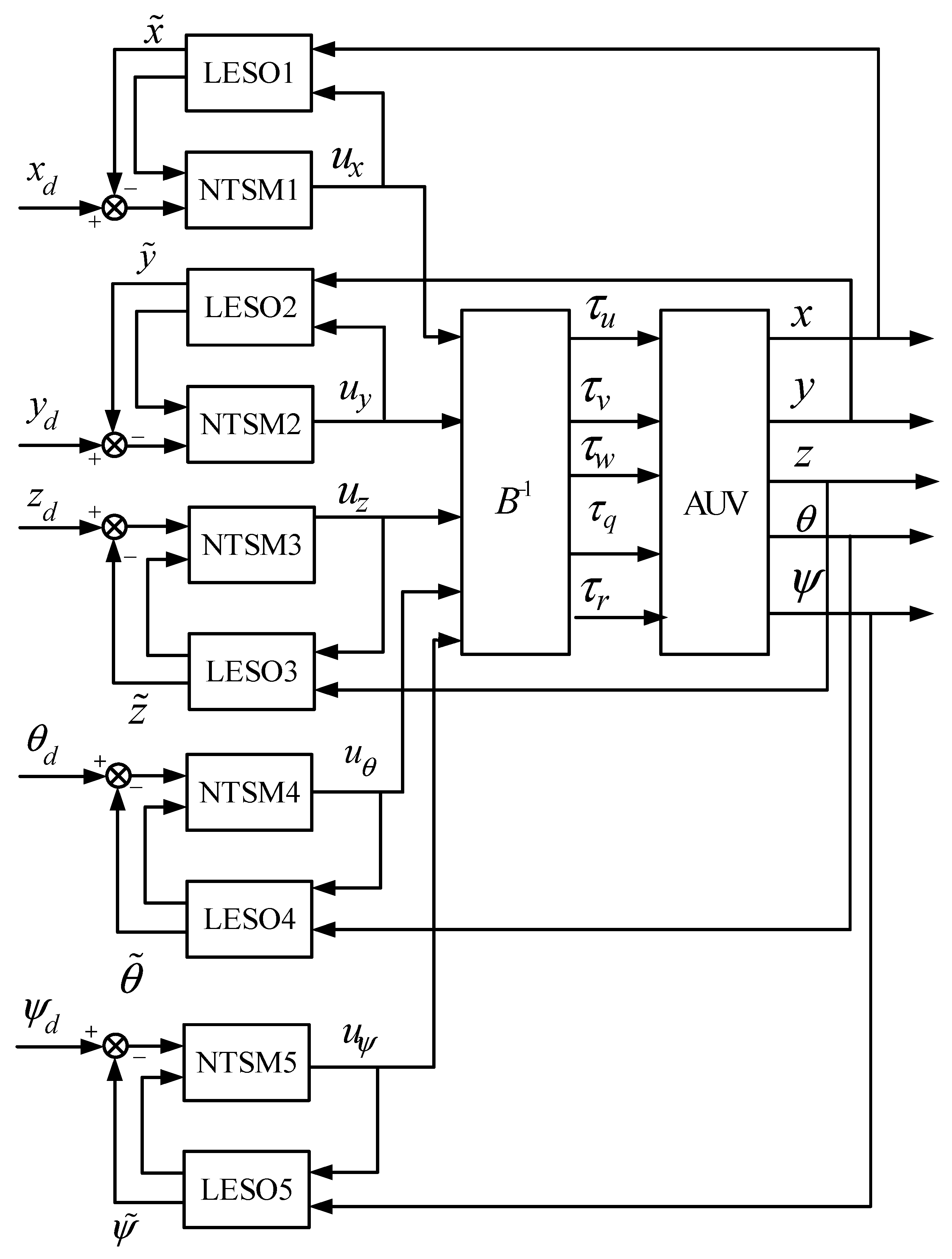
3. Three-Dimensional Trajectory Tracking Controller Design

After the above discussion, the basic framework of the decoupling control of the AUV system based on ADRC technology has been initially developed. In this section, we will introduce the design process of the AUV 3D trajectory tracking controller based on the NTSM-ADRDC. The total control framework of the proposed algorithm is depicted in Figure 4. The control frame is divided into five channels: x d x ,   y d y ,   z d z ,   θ d θ and ψ d ψ , among which each channel is an independent SISO system. The LESO has strong ability to observe the total disturbance of AUV system, and the introduction of the exponential reaching law in NTSM allows for faster convergence of tracking errors. The close combination of the methods constitutes the NTSM-ADRDC controller.

3.1. Linear Extended State Observer Design

As the core component of LADRC algorithm, the LESO can estimate the internal uncertain dynamics and external disturbances according to the input–output states of the system. Taking the position state x of AUV as an example, according to Equation (12), the f 1 ( u , v , r , ψ ) + w 1 is regarded by LESO1 as the total disturbances of the x d x channel in AUV system, which can be expanded into the new state variable x 3 , namely x 3 = f 1 ( u , v , r , ψ ) + w 1 , and let x 1 = x , x ˙ 3 = h 1 . Where the h1 denotes the derivative of the total disturbance observed by LESO1. Therefore, the equation of x ¨ in the system (12) can be expanded into the following control system:
{ x ˙ 1 = x 2 x ˙ 2 = x 3 + u x x ˙ 3 = h 1 y = x 1
Next, we can construct LESO1 according to Equation (13)
{ x ˜ ˙ 1 = x 2 β 01 ( x ˜ 1 x 1 ) x ˜ ˙ 2 = x 3 β 02 ( x ˜ 1 x 1 ) + u x x ˜ ˙ 3 = β 03 ( x ˜ 1 x 1 )
Here x ˜ 1 , x ˜ 2 , x ˜ 3 are the estimated values of x 1 , x 2 , x 3 , respectively, and β 01 , β 02 , β 03 are the gains of the LESO1. According to the characteristics of linear ESO, β 01 , β 02 , β 03 have the following relationship:
[ β 01 β 02 β 03 ] = [ 3 ω 0 3 ω 0 2 ω 0 3 ]
where ω 0 is often called the observer bandwidth. Note that there is a LESO1 estimation error between the estimated values x ˜ i and actual values x i ( i = 1 , 2 , 3 ) , but the estimation error is able to converge to 0 according to the literature [35,36]. The remaining three channels of LESO can be designed as follows:
{ y ˜ ˙ 1 = y ˜ 2 β 01 ( y ˜ 1 y 1 ) y ˜ ˙ 2 = y ˜ 3 β 02 ( y ˜ 1 y 1 ) + u y y ˜ ˙ 3 = β 03 ( y ˜ 1 y 1 )
{ z ˜ ˙ 1 = z ˜ 2 β 01 ( z ˜ 1 z 1 ) z ˜ ˙ 2 = z ˜ 3 β 02 ( z ˜ 1 z 1 ) + u z z ˜ ˙ 3 = β 03 ( z ˜ 1 z 1 )
{ θ ˜ ˙ 1 = θ ˜ 2 β 01 ( θ ˜ 1 θ 1 ) θ ˜ ˙ 2 = θ ˜ 3 β 02 ( θ ˜ 1 θ 1 ) + u θ θ ˜ ˙ 3 = β 03 ( θ ˜ 1 θ 1 )
{ ψ ˜ ˙ 1 = ψ ˜ 2 β 01 ( ψ ˜ 1 ψ 1 ) ψ ˜ ˙ 2 = ψ ˜ 3 β 02 ( ψ ˜ 1 ψ 1 ) + u ψ ψ ˜ ˙ 3 = β 03 ( ψ ˜ 1 ψ 1 )
where y ˜ i , z ˜ i , θ ˜ i , ψ ˜ i ( i = 1 , 2 , 3 ) are the state estimates of y i , z i , θ i , ψ i ( i = 1 , 2 , 3 ) , respectively.

3.2. Design of NTSM Nonlinear States Error Feedback Control Law

Combined with LESO’s observation ability to system state variables and total disturbance, the NTSM nonlinear states error feedback control law will be designed. Its key idea is to use LESO to improve the control law by real-time estimates of the AUV’s internal uncertain dynamics and external disturbance. On the premise of ensuring the advantages of LADRC, it improves the robustness of the controller. In addition, the exponential reaching law is introduced to enhance the convergence speed of the system tracking error.
To ensure that the tracking error in the x d x channel converges to zero in finite time, and to solve the singularity problem in terminal sliding mode control, we choose the following non-singular terminal sliding surface [29]:
S x = e x + 1 β 1 sgn ( e ˙ x ) | e ˙ x | λ 1
where e x = x 1 x d , e ˙ x = x 2 x ˙ d . Since LESO1 can observe the estimated value of state variable x , we can rewrite it as e x x ˜ 1 x d , e ˙ x x ˜ 2 x ˙ d . β 1 , and λ 1 are adjustable parameters, satisfying β 1 > 0 , 1 < λ 1 < 2 .
From the derivation of Equation (20),
S ˙ x = e ˙ x + λ 1 β 1 | e ˙ x | λ 1 1 e ¨ x = e ˙ x + λ 1 β 1 | e ˙ x | λ 1 1 ( f 1 ( u , v , r , ψ ) + w 1 + u x - x ¨ d )
Here, we introduce the exponential reaching law,
S ˙ x = k 1 S x ε 1 tanh ( S x )
Among them, the first term is to use the exponential to shorten the convergence time, and the second term uses the function tanh ( . ) to weaken the system chattering [37], satisfying k 1 > 0 , ε 1 > 0 .
Combining Equations (21) and (22), we can conclude that
e ˙ x + λ 1 β 1 | e ˙ x | λ 1 1 ( f 1 ( u , v , r , ψ ) + w 1 + u x - x ¨ d ) = k 1 S x ε 1 tanh ( S x )
Let ρ ( e ˙ x ) = λ 1 β 1 | e ˙ x | λ 1 1 , according to the Equation (23), the NTSM control based on the exponential reaching law can be deduced as:
u x = ρ ( e ˙ x ) 1 ( k 1 S x + ε 1 tanh ( S x ) + e ˙ x ) ( f 1 ( u , v , r , ψ ) + w 1 x ¨ d )
Considering that the control law (24) contains ρ ( e ˙ ξ ) = λ 1 β 1 | e ˙ ξ | λ 1 1 term that will cause a relatively large amount of calculation, we can simplify the control law on the basis of ensuring the reaching law and the simplified control law can be described as:
u x = ( β 1 λ 1 sgn ( e ˙ x ) | e ˙ x | 2 λ 1 + J 1 S x + σ LESO 1 tanh ( S x ) + f 1 ( u , v , r , ψ ) + w 1 x ¨ d )
where J 1 > 0 and σ LESO 1 > 0 , σ LESO 1 is the upper bound of the observation error of LESO1 to the uncertainty.
Since x ˜ 3 is LESO1′s real-time estimated value of the sum of internal dynamics and external disturbances of the AUV channel x d x , it can be obtained that
x ˜ 3 = f 1 ( u , v , r , ψ ) + w 1
Substituting Equation (26) into Equation (25), the nonlinear states error feedback control law of channel x d x can finally be expressed as:
u x = ( β 1 λ 1 sgn ( e ˙ x ) | e ˙ x | 2 λ 1 + J 1 S x + σ LESO 1 tanh ( S x ) + x ˜ 3 x ¨ d )
Similarly, the sliding mode surfaces of the remaining three channels can be chosen as:
{ S y = e y + 1 β 2 sgn ( e ˙ y ) | e ˙ y | λ 2 S z = e z + 1 β 3 sgn ( e ˙ z ) | e ˙ z | λ 3 S θ = e θ + 1 β 4 sgn ( e ˙ θ ) | e ˙ θ | λ 4 S ψ = e ψ + 1 β 5 sgn ( e ˙ ψ ) | e ˙ ψ | λ 5
where
{ e y = y ˜ 1 y d e z = z ˜ 1 z d e θ = θ ˜ 1 θ d e ψ = ψ ˜ 1 ψ d
{ e ˙ y = y ˜ 2 y ˙ d e ˙ z = z ˜ 2 z ˙ d e ˙ θ = θ ˜ 2 θ ˙ d e ˙ ψ = ψ ˜ 2 ψ ˙ d
The nonlinear error control law of the remaining four channels can be designed as follows:
{ u y = ( β 2 λ 2 | e ˙ y | 2 λ 2 + J 2 S y + σ LESO 2 tanh ( S y ) + y ˜ 3 y ¨ d ) u z = ( β 3 λ 3 | e ˙ z | 2 λ 3 + J 3 S z + σ LESO 3 tanh ( S z ) + z ˜ 3 z ¨ d ) u θ = ( β 4 λ 4 | e ˙ θ | 2 λ 4 + J 4 S θ + σ LESO 4 tanh ( S θ ) + θ ˜ 3 θ ¨ d ) u ψ = ( β 5 λ 5 | e ˙ ψ | 2 λ 5 + J 5 S ψ + σ LESO 5 tanh ( S ψ ) + ψ ˜ 3 ψ ¨ d )

3.3. System Stability Analysis

Assumption 1.
The reference trajectory of AUV system η d = [ x d y d z d θ d ψ d ] T are bounded.
Theorem 2.
For the 5-DOF AUV system, considering the model (12), LESO (14)–(19), and the control laws Equations (27) and (31), then there exist control parameters satisfying β i > 0 , 1 < λ i < 2 , J i > 0 , and σ LESO i > 0   ( i = 1 , 2 , 5 ) , such that the closed-loop system is stable.
Proof. 
Construct the Lyapunov function of the AUV system as:
V = V x + V y + V z + V θ + V ψ = 1 2 S x 2 + 1 2 S y 2 + 1 2 S z 2 + 1 2 S θ 2 + 1 2 S ψ 2
According to Lyapunov stability theory, AUV system is stable if the condition of V = s s ˙ 0 is satisfied. Therefore, the derivative of the Equation (21) is as follows:
V ˙ = V ˙ x + V ˙ y + V ˙ z + V ˙ θ + V ˙ ψ = S x S ˙ x + S y S ˙ y + S z S ˙ z + S θ S ˙ θ + S ψ S ˙ ψ
where
V ˙ x = S x S ˙ x = S x [ e ˙ x + λ 1 β 1 | e ˙ x | λ 1 1 ( f 1 ( u , v , r , ψ ) + w 1 + u x - x ¨ d ) ]           = S x { e ˙ x + λ 1 β 1 | e ˙ x | λ 1 1 [ f 1 ( u , v , r , ψ ) + w 1 - x ¨ d - ( β 1 λ 1 sgn ( e ˙ x ) | e ˙ x | 2 λ 1 + J 1 S x + σ LESO 1 tanh ( S x ) + x ˜ 3 x ¨ d ) ] }           = S x [ e ˙ x λ 1 β 1 | e ˙ x | λ 1 1 ( β 1 λ 1 sgn ( e ˙ x ) | e ˙ x | 2 λ 1 + J 1 S x + σ LESO 1 tanh ( S x ) ] = S x [ λ 1 β 1 | e ˙ x | λ 1 1 ( J 1 S x + σ LESO 1 tanh ( S x ) ) ]           = λ 1 β 1 | e ˙ x | λ 1 1 ( J 1 S x 2 + σ LESO 1 S x tanh ( S x ) )
Since β 1 > 0 and 1 < λ 1 < 2 , so λ 1 β 1 | e ˙ x | λ 1 1 0 . In addition, because of S x tanh ( S x ) 0 , S x 2 0 , we can conclude that V ˙ x 0 .
In a similar way, we can derive the following results:
V ˙ = V ˙ x + V ˙ y + V ˙ z + V ˙ θ + V ˙ ψ 0

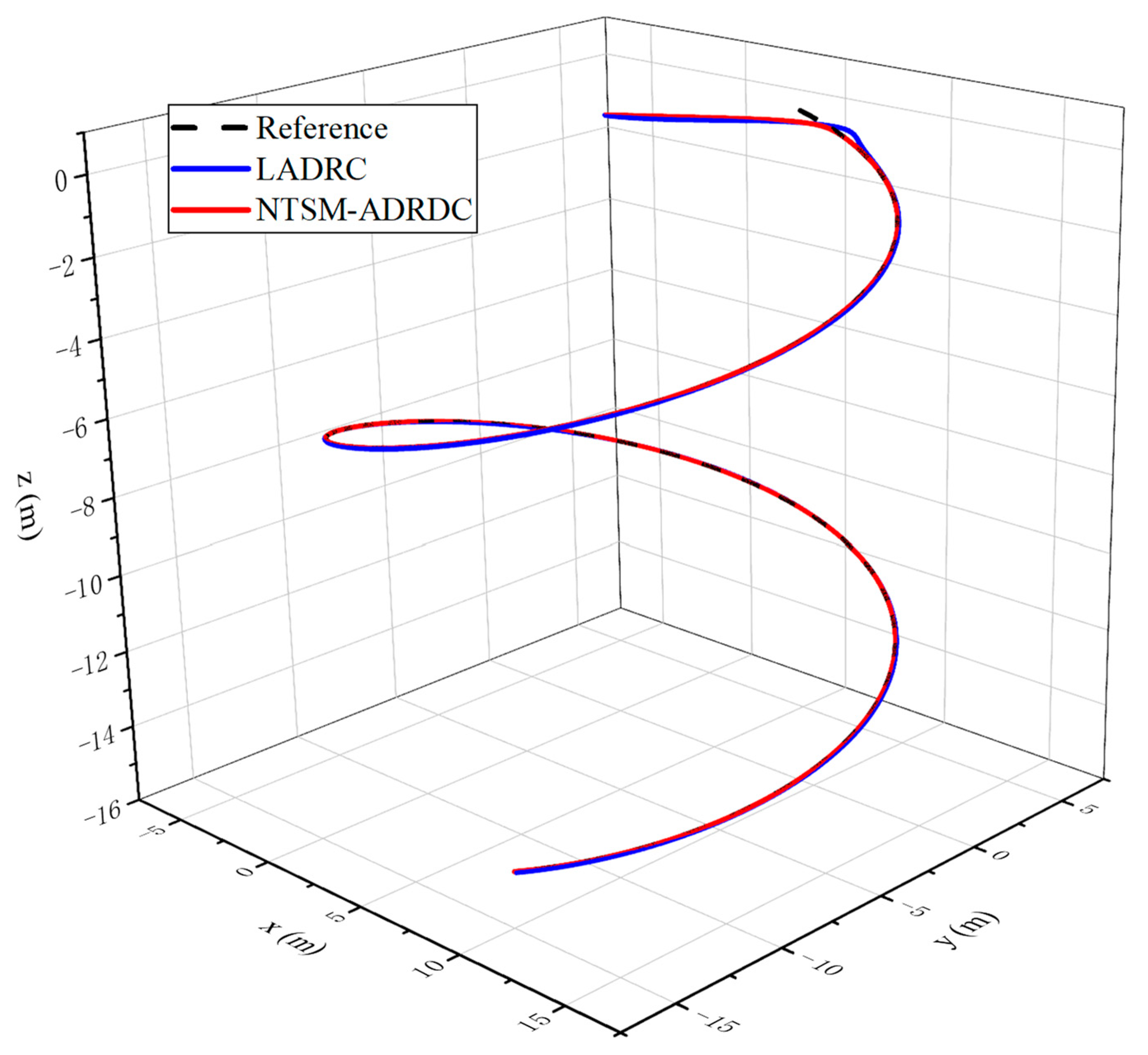
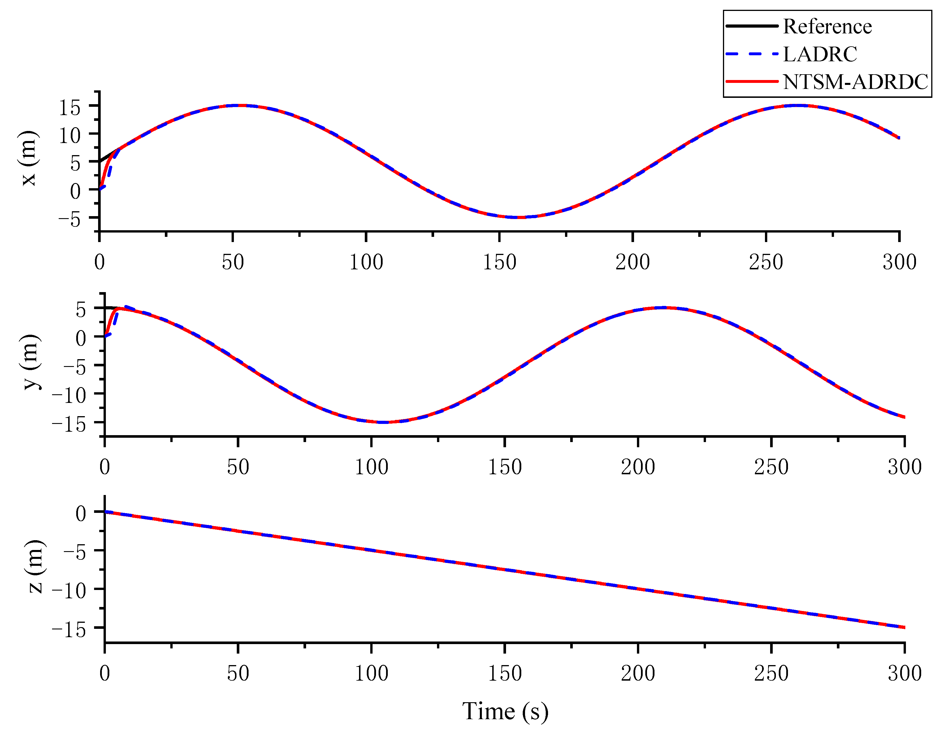
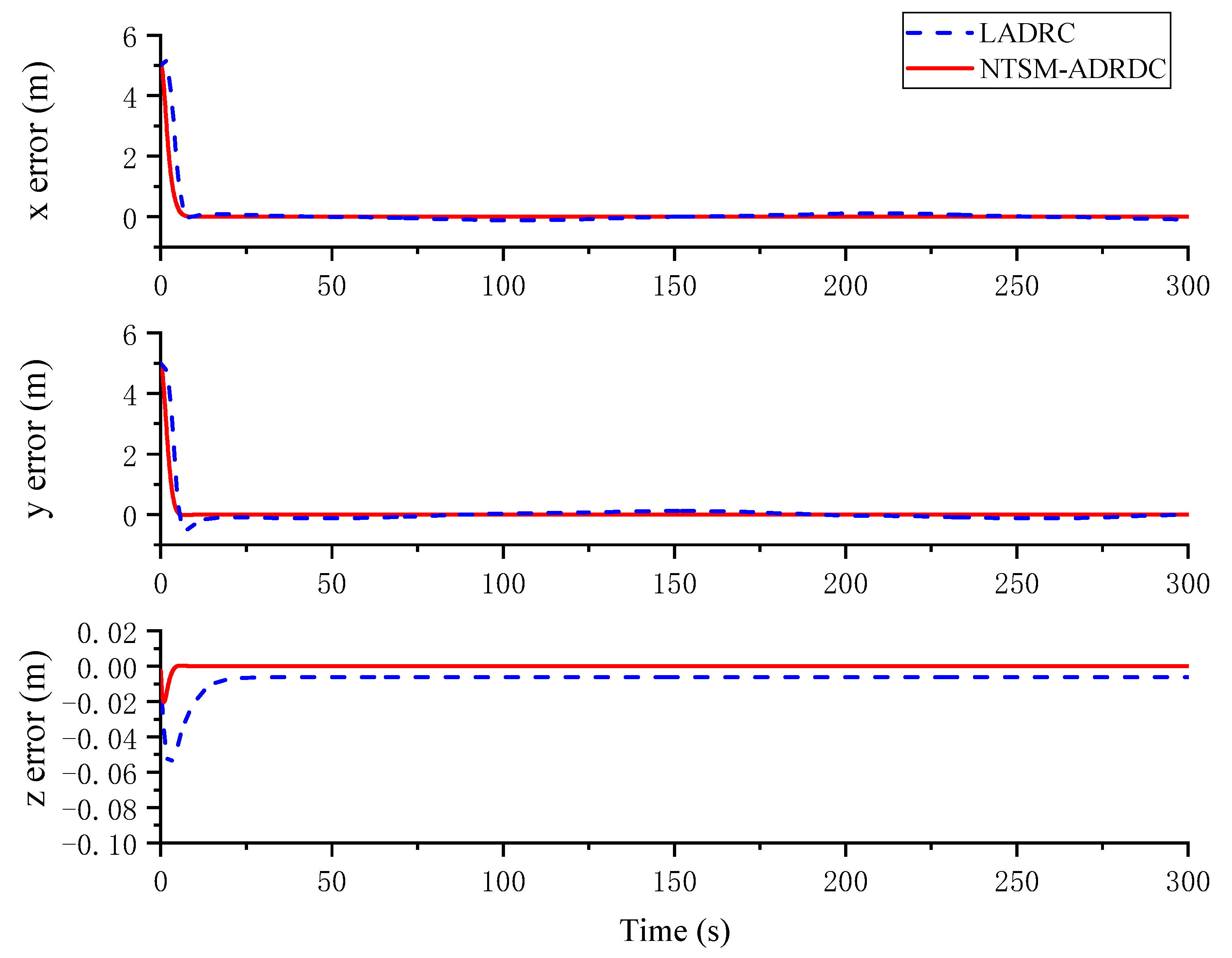
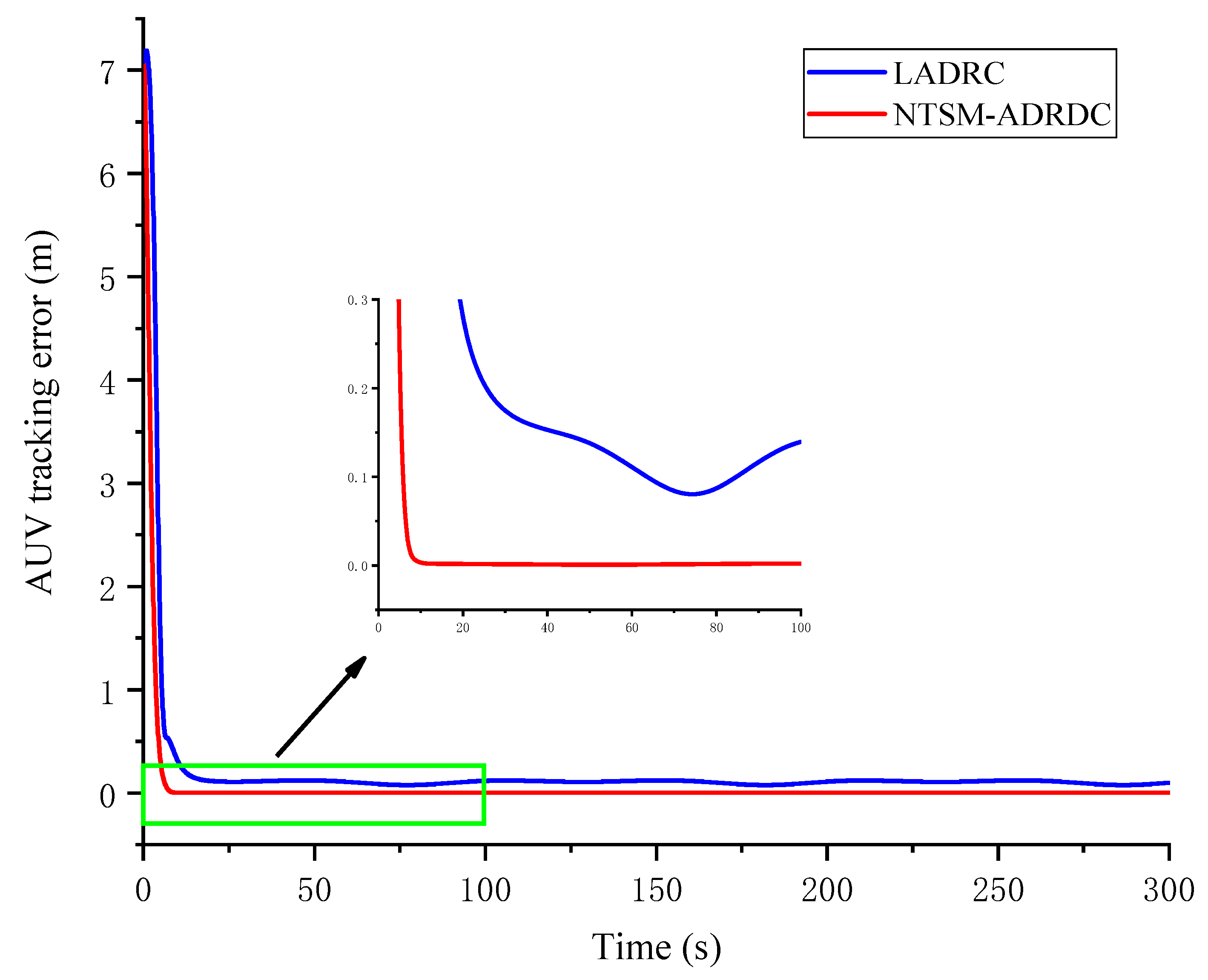
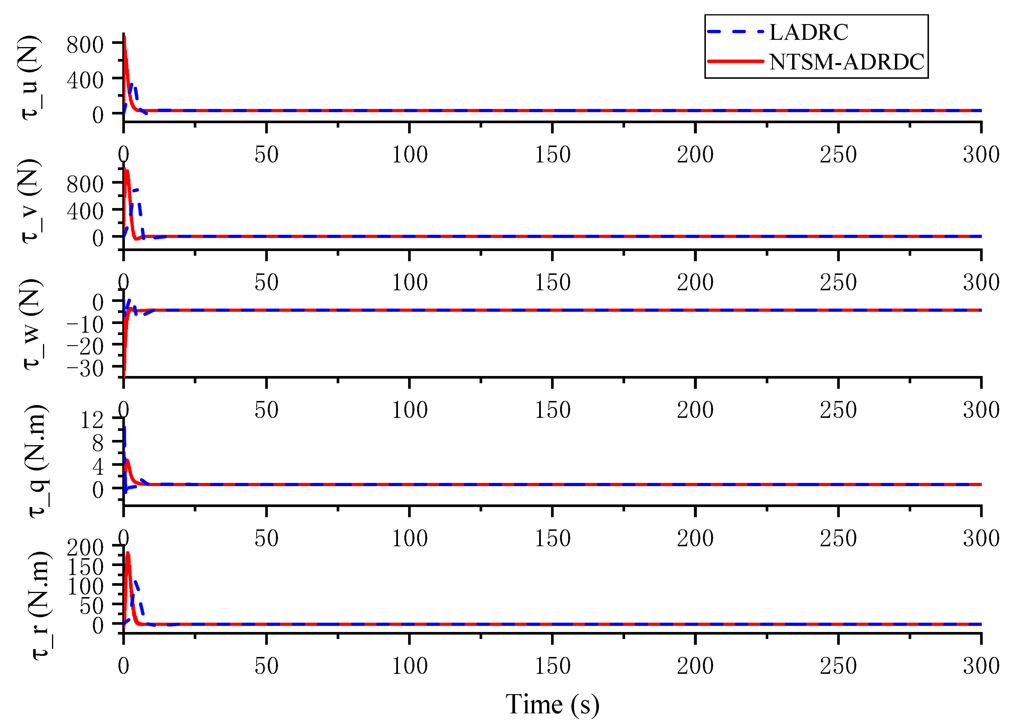
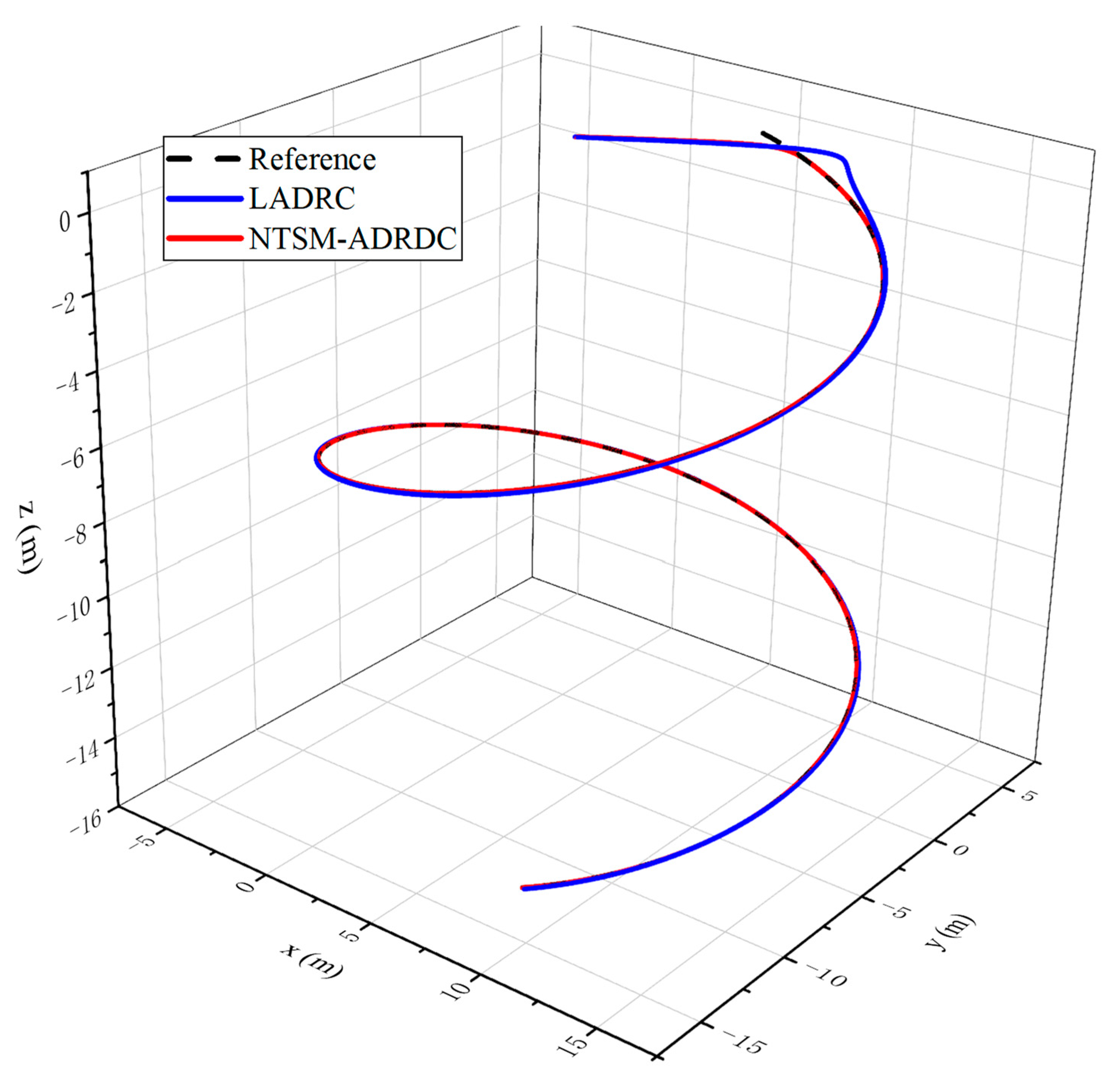
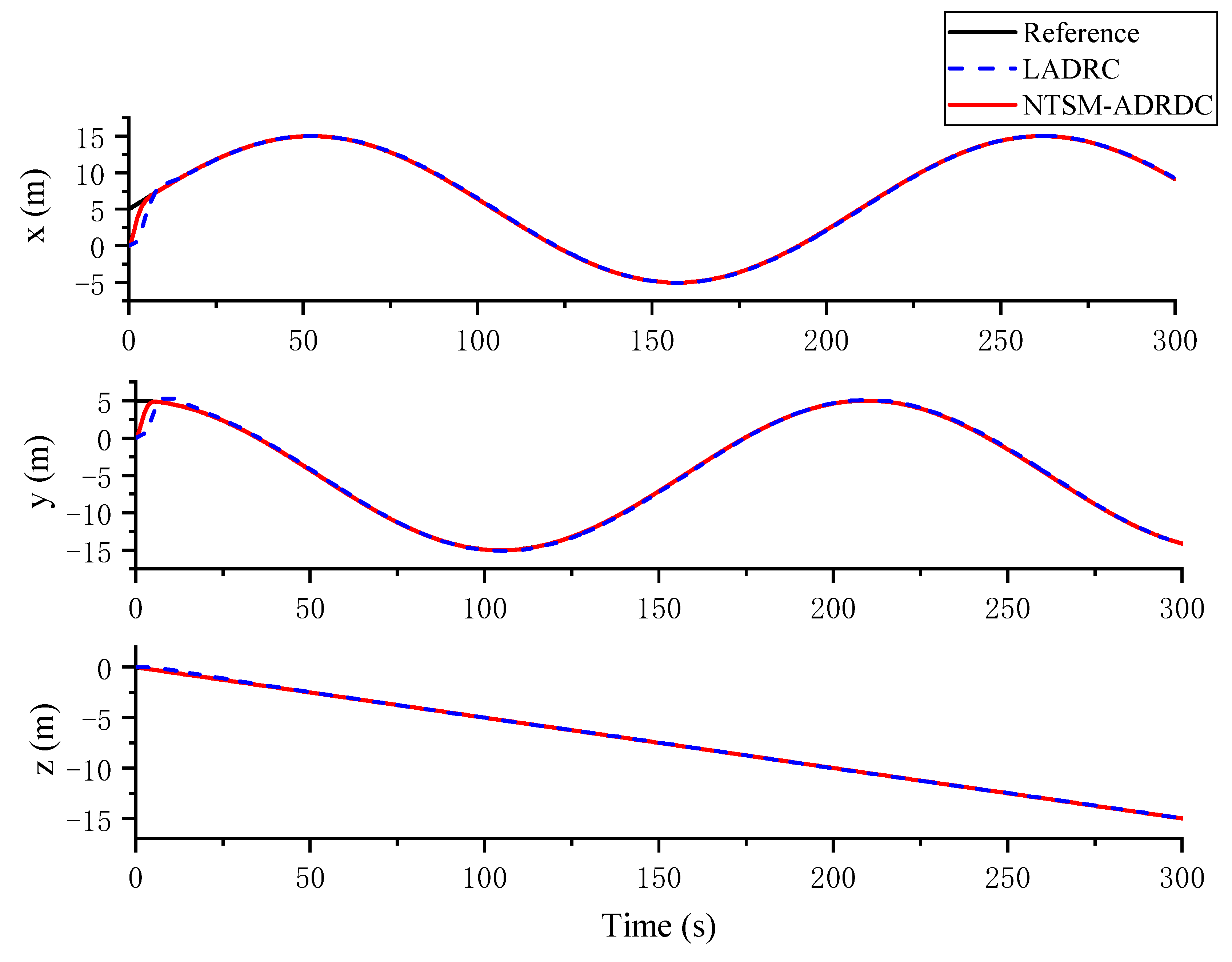
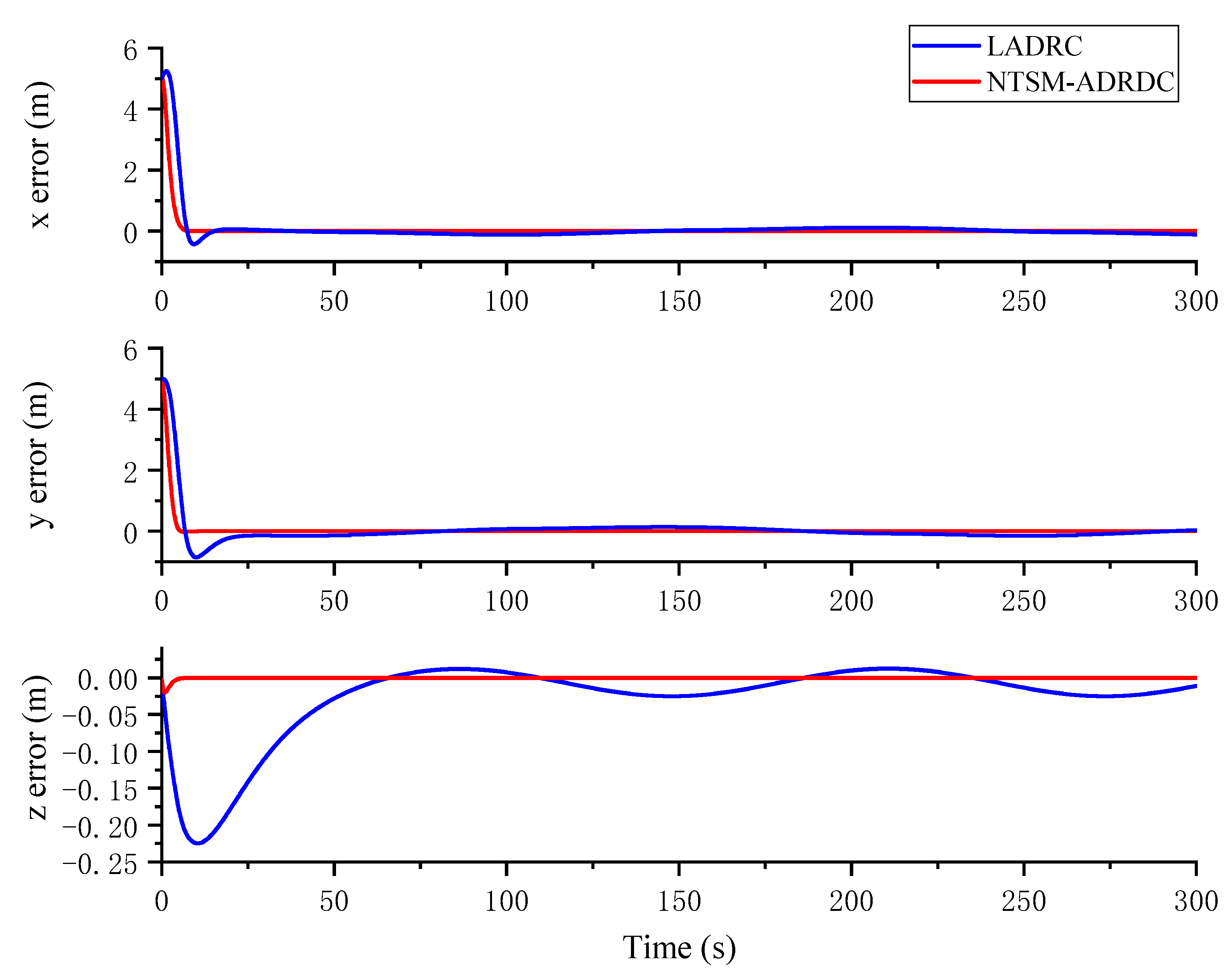
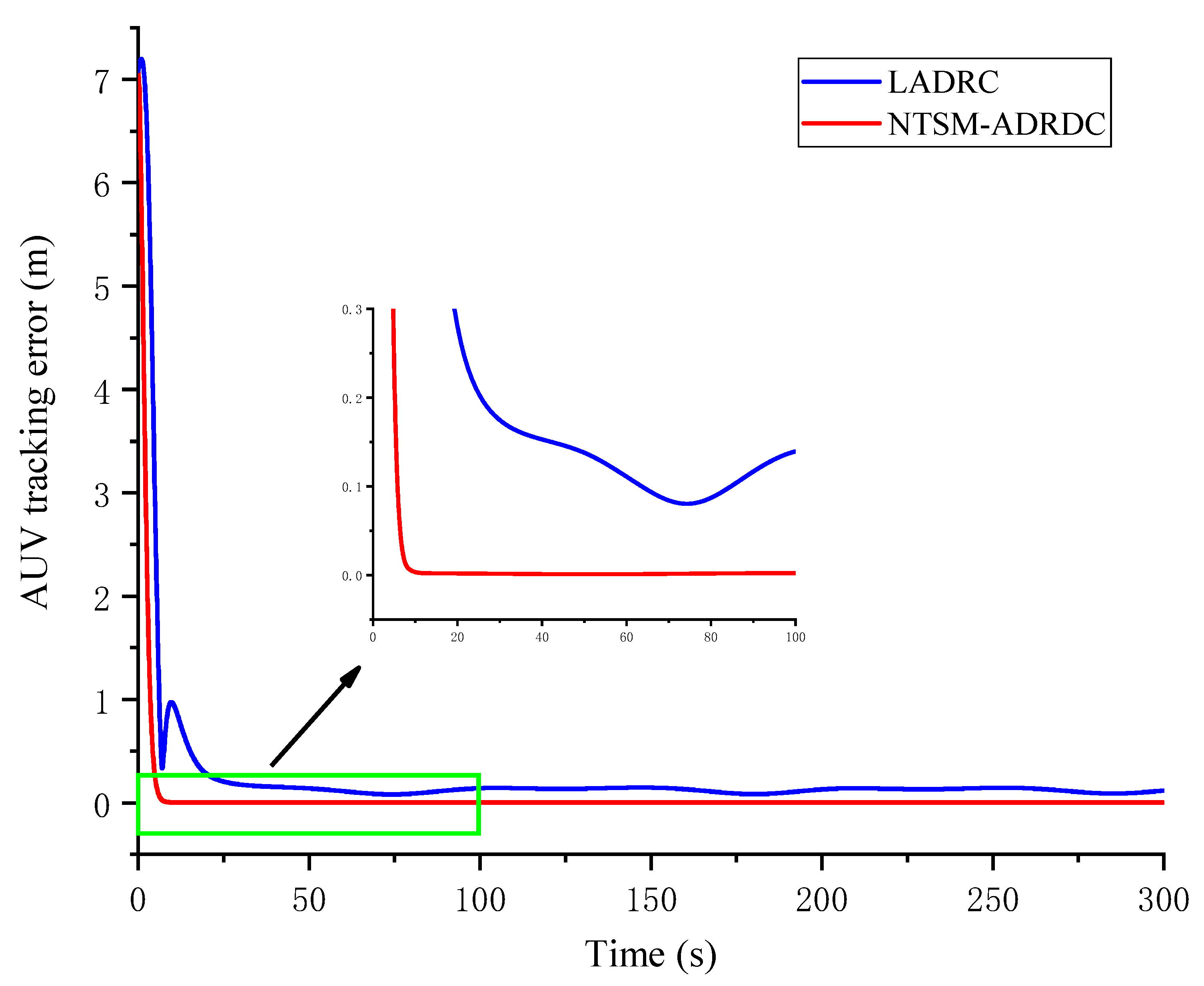
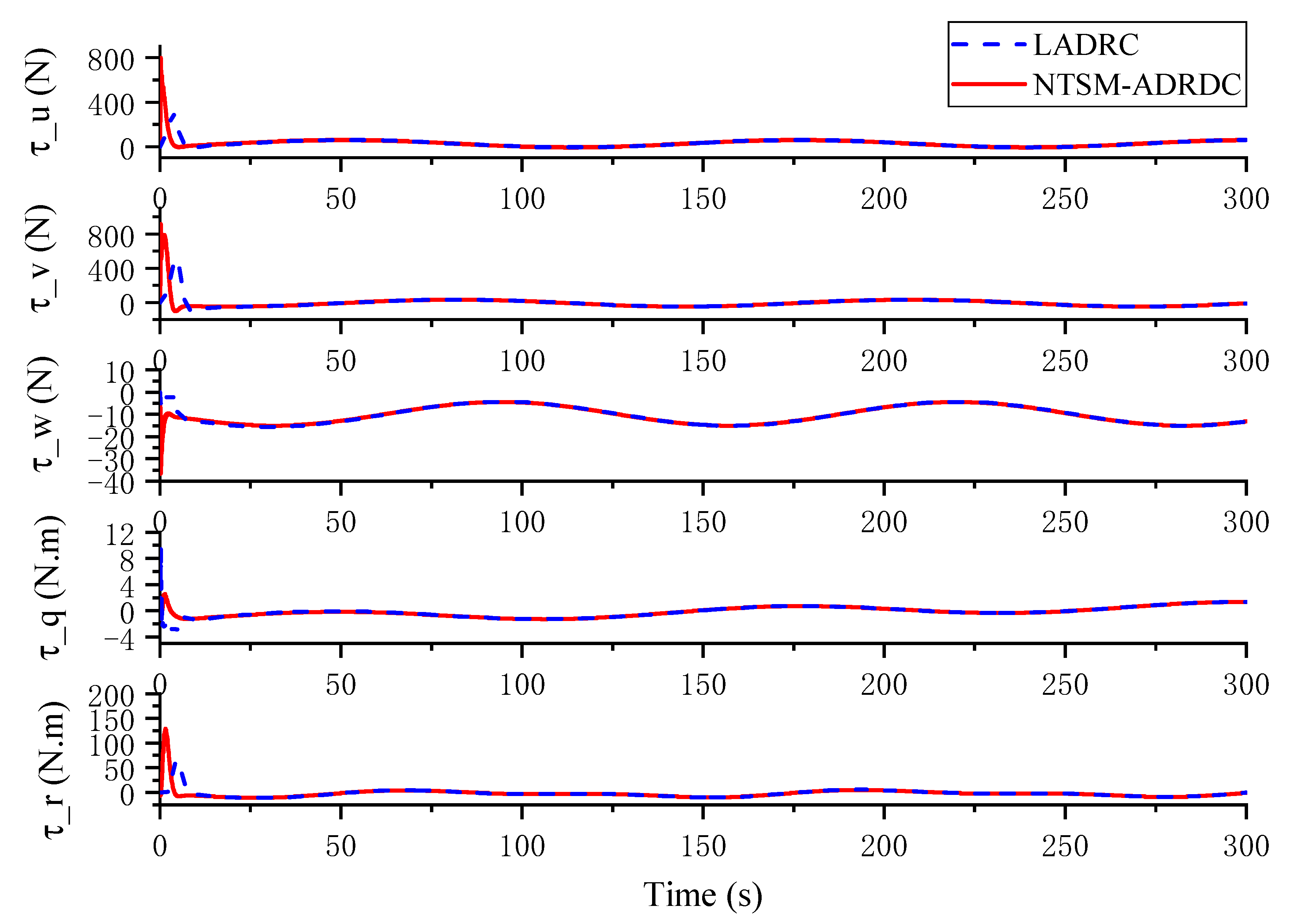
4. Simulation Results and Analysis

To verify the effectiveness of the NTSM-ADRDC algorithm proposed in this paper, the AUV 3D trajectory tracking simulation is studied in this section. By comparing with the LADRC method, the proposed control strategy has better performance in control accuracy, anti-disturbance, and robustness. The control laws for the NTSM-ADRDC algorithm are Equations (27) and (31). A detailed introduction to the LDARC method can be referred to in the literature [24]. The detailed hydrodynamic parameter values of AUV as shown in Table 1.
The control parameters of the NTSM-ADRDC controller in the simulation are selected as: h = 0.05, ω 0 = 15; β 1 = 0.60, λ 1 = 15/13, J 1 = 0.60, σ LESO 1 = 1.00; β 2 = 0.75, λ 2 = 13/11, J 2 = 0.65, σ LESO 2 = 0.85; β 3 = 0.55, λ 3 = 15/13, J 3 = 0.75, σ LESO 3 = 0.80; β 4 = 0.25, λ 4 = 11/9, J 4 = 0.50, σ LESO 4 = 0.52; β 5 = 0.20, λ 5 = 17/15, J 5 = 0.50, σ LESO 5 = 0.55; AUV initial state η 0 = [ 0 0 0 0 0 ] T . In the simulation, the method of determining the bandwidth ω 0 of the LESO can be found in the literature [38]. The control parameter λ i can be determined first since it has little effect on the control effect as long as it satisfies 1 < λ i < 2 . Then, the value range of β i is constrained to be between 0 and 1. Finally, the larger the parameters of σ LESOi and J i , the faster the convergence rate. However, the “chattering” phenomenon may be generated as the values of σ LESOi and J i increase. Therefore, it is necessary to trade off between suppressing “chattering” and speeding up the convergence rate. Usually, we choose a slightly larger value of σ LESOi than J i to weaken the “chattering”.
AUV three-dimensional tracking reference trajectory is defined as:
{ x d = 5 + 10 sin ( 0.03 t ) y d = 5 + 10 cos ( 0.03 t ) z d = 0.05 t θ d = 0.03 ψ d = 0.03 t
Figure 5 shows the three-dimensional trajectory curves of two different control algorithms without disturbance. The cylindrical spiral is used as the reference trajectory to simulate the tracking of the spiral diving target by the AUV. The black dotted line represents the reference trajectory. The blue solid line represents the AUV tracking result under the LADRC algorithm. The red solid line represents the simulation result of the designed NTSM-ADRDC. It can be seen from the figure that the three-dimensional trajectory curves of the two control algorithms without disturbance are consistent with the reference trajectory. It shows that although the initial position of the AUV is far from the reference trajectory, both methods can track the reference trajectory more accurately and quickly. However, there is an overshoot in NTSM-ADRDC compared to LADRC. The position tracking performance of the AUV is shown in Figure 6. We can observe that both control algorithms show good trajectory tracking performance.
The position tracking performance of the AUV is shown in Figure 6. We can observe that the two control algorithms can follow the corresponding reference trajectory curve well. Through the comparison of the first 20 s, it can be clearly found that the NTSM-ADRDC algorithm can approach the desired position faster. By comparing the position error of the two control methods in Figure 7, can we discover NTSM-ADRDC has a faster error convergence rate than LADRC.
In order to reflect the trajectory tracking accuracy of different controllers, we define the AUV trajectory tracking error in the 3D space as follows:
E η ( t ) = ( x ( t ) x d ( t ) ) 2 + ( y ( t ) y d ( t ) ) 2 + ( z ( t ) z d ( t ) ) 2
where x ( t ) , y ( t ) , z ( t ) are the actual position values of the AUV at the time t , and x d ( t ) , y d ( t ) , z d ( t ) represent the desired position values at the time t .
Figure 8 shows the comparison curve of AUV trajectory tracking error. Since the initial position of the AUV is far from the starting point of the reference position, it takes a certain time for the AUV to make the trajectory tracking error tend to 0. The AUV tracking error tends to zero after approximately 8 s under the ATSM-ADRDC algorithm, while LADRC is about 20 s. This shows that the error convergence time of the former is shorter than that of the latter. From the partial enlargement, we can clearly see that the trajectory tracking error of ATSM-ADRDC converges more smoothly compared to LADRC.
To further evaluate the tracking error accuracy of the AUV under the two controllers, we introduce three indicators related to the tracking error: the maximum tracking error (Max), the minimum tracking error (Min), and the average tracking error (Avg). The tracking error measurement values after 20 s are shown in Table 2. Taken together, it can be concluded that the control accuracy of NTSM-ADRDC is much higher than that of LADRC. As can be seen from Figure 9, the proposed NTSM-ADRC scheme has almost no “chattering” in the control inputs. It also indicates that the use of the tanh function to replace the sign function can reduce “chattering”.
Based on the above analysis, both controllers can track the reference trajectory well in the absence of disturbance. In comparison, the trajectory following performance of NTSM-ADRDC is significantly better than LADRC. The main reason is that the former combines the exponential approach law (22), which ensures the rapid error convergence of the designed algorithm in a finite time.
In order to analyze the anti-disturbance performance of the designed algorithm, ocean current and bounded disturbances are added to the simulation. Ocean current disturbance in I-frame: u c I = 0.25 m/s, v c I = 0.25 m/s. External bounded disturbances:
d u = 0.02 m 11 [ 1 + sin ( 0.05 t ) ] ,         d v = 0.02 m 22 [ 1 + sin ( 0.05 t ) ] , d w = 0.02 m 33 [ 1 + sin ( 0.05 t ) ] ,         d q = 0.01 m 55 [ 1 + cos ( 0.01 t ) ] , d r = 0.01 m 66 [ 1 + cos ( 0.01 t ) ] .
Figure 10 shows the AUV 3D trajectory curves of the two control algorithms with the disturbance. We can find that both control approaches can still track the reference trajectory relatively well in the presence of disturbances. Nevertheless, the LADRC produces significant overshoot. From Figure 11 we can observe that the NTSM-ADRDC algorithm not only allows a faster approach to the desired position, but also without overshoot.
By comparing the position error under the two control algorithms, we can find from Figure 12 that the algorithm designed in this paper still has a faster error convergence rate with the disturbance, which shows that the exponential reaching law introduced into the NTSM-ADRDC algorithm is effective in the presence of disturbance. From Figure 13, we can clearly find that the AUV tracking error tracking convergence time is approximately 10 s under the ATSM-ADRDC algorithm, while LADRC is about 26 s. This shows that the proposed NTSM-ADRDC method has a faster error convergence compared to the LADRC. Additionally, the partial enlargement shows that there are larger fluctuations in the LADRC method compared to NTSM-ADRDC. It shows that the stability of NTSM-ADRDC is much better than that of the latter.
The tracking error measurement values after 26 s are shown in Table 3. In the presence of disturbance, the average of the tracking error of NTSM-ADRDC is 0.00162 m, while LADRC is about 0.12461 m. This indicates that the designed controller has high control accuracy in the presence of ocean currents and external disturbances. Figure 14 shows the control input of AUV with disturbance. We can see that there is some fluctuation in the control input due to the presence of ocean currents and external disturbances.
Based on the above analysis, the designed algorithm has good robustness and anti-disturbance. There are two main reasons: one is that ADRC technology can effectively suppress model uncertainty and external disturbance, and the other is that the combination of NTSM and the exponential reaching law not only retains strong robustness but also can ensure the rapid convergence of tracking errors in a finite time.

5. Conclusions

Aiming at the problem of AUV trajectory tracking control, this paper designs a novel tracking control method based on NTSM-ADRDC. Firstly, the AUV 5-DOF model is decoupled by introducing the ADRC technology. Secondly, the 3D trajectory tracking controller based on NTSM-ADRDC is designed. The controller uses LESO to observe the state variable values of the AUV and estimate the sum of the unmodeled dynamics and external disturbances of the system. By introducing the exponential reaching law into NTSM, a nonlinear error feedback law is designed to compensate for the total disturbance of the system. Combining NTSMC and ADRC technology can retain the advantages of the two control algorithms to the maximum. The NTSMC strategy can make the AUV quickly approach the reference trajectory, and the ADRC can suppress model uncertainty and external disturbance. Finally, the simulation verifies the effectiveness of the designed controller by comparing it with LADRC.
In future work, we will investigate the theory of optimization of the control parameters of the NTSM-ADRDC algorithm to improve the engineering applicability of the designed algorithm. Meanwhile, considering the input and state constraints existing in the AUV system, we will combine other methods, such as model predictive control, in the design process of the ADRC controller. In addition, in order to match the configuration of AUV actuators in actual applications, thrust allocation schemes will be investigated for the design of the controller.

Author Contributions

Methodology, W.W.; Validation, Z.Y.; Investigation, Z.L.; Data curation, X.D.; Writing—original draft, W.W.; Writing—review & editing, W.W.; Funding acquisition, W.Z. All authors have read and agreed to the published version of the manuscript.

Funding

This work was supported by the National Natural Science Foundation of China under grant E1102/52071108, and in part by National Natural Science Foundation of China under grant 5217110332, and the Natural Science Foundation of Heilongjiang Province under grant JJ2021JQ0075.

Institutional Review Board Statement

Not applicable.

Informed Consent Statement

Not applicable.

Data Availability Statement

Not applicable.

Conflicts of Interest

The authors declare no conflict of interest.

References

  1. Wynn, R.B.; Huvenne, V.A.; Le Bas, T.P.; Murton, B.J.; Connelly, D.P.; Bett, B.J. Autonomous Underwater Vehicles (AUVs): Their past, present and future contributions to the advancement of marine geoscience. Mar. Geol. 2014, 352, 451–468. [Google Scholar] [CrossRef]
  2. Palomeras, N.; Vallicrosa, G.; Mallios, A.; Bosch, J.; Vidal, E.; Hurtos, N.; Carreras, M.; Ridao, P. AUV homing and docking for remote operations. Ocean Eng. 2018, 154, 106–120. [Google Scholar] [CrossRef]
  3. An, L.; Li, Y.; Cao, J.; Jiang, Y.; He, J.; Wu, H. Proximate time optimal for the heading control of underactuated autonomous underwater vehicle with input nonlinearities. Appl. Ocean Res. 2020, 95, 102002. [Google Scholar] [CrossRef]
  4. Yan, Z.; Yu, H.; Zhang, W. Globally finite-time stable tracking control of underactuated UUVs. Ocean Eng. 2015, 107, 106–120. [Google Scholar] [CrossRef]
  5. Yan, Z.; Gong, P.; Zhang, W.; Wu, W.H. Model predictive control of autonomous underwater vehicles for trajectory tracking with external disturbances. Ocean Eng. 2020, 217, 107884. [Google Scholar] [CrossRef]
  6. Li, Y.; Jiang, Y.Q.; Wang, L.F.; Cao, J.; Zhang, G.C. Intelligent PID guidance control for AUV path tracking. J. Cent. South Univ. 2015, 22, 3440–3449. [Google Scholar] [CrossRef]
  7. Robert, S.M.; Brett, W.H.; Lance, M. Docking control system for a 54-cm-diameter (21-in) AUV. IEEE J. Oceanic. Eng. 2009, 33, 550–562. [Google Scholar]
  8. Liang, X.; Qu, X.; Wang, N. Three-Dimensional Trajectory Tracking of an Underactuated AUV based on Fuzzy Dynamic Surface Control. IET Intell. Transp. Syst. 2019, 14, 364–370. [Google Scholar] [CrossRef]
  9. Yin, J.C.; Wang, N. Predictive Trajectory Tracking Control of Autonomous Underwater Vehicles Based on Variable Fuzzy Predictor. Int. J. Fuzzy Syst. 2020, 23, 1809–1822. [Google Scholar] [CrossRef]
  10. Rezazadegan, F.; Shojaei, K.; Sheikholeslam, F.; Chatraei, A. A novel approach to 6-DOF adaptive trajectory tracking control of an AUV in the presence of parameter uncertainties. Ocean Eng. 2015, 107, 246–258. [Google Scholar] [CrossRef]
  11. Guerrero, J.; Torres, J.; Creuze, V.; Chemori, A. Adaptive disturbance observer for trajectory tracking control of underwater vehicles. Ocean Eng. 2020, 200, 107080. [Google Scholar] [CrossRef]
  12. Park, B.S. Neural Network-Based Tracking Control of Underactuated Autonomous Underwater Vehicles with Model Uncertainties. J. Dyn. Syst.-T Asme. 2015, 137, 021004. [Google Scholar] [CrossRef]
  13. Eski, K.; Yldrm, S. Design of Neural Network Control System for Controlling Trajectory of Autonomous Underwater Vehicles. Int. J. Adv. Robot. Syst. 2014, 11, 1–17. [Google Scholar] [CrossRef]
  14. Zhang, Y.D.; Liu, X.F.; Liu, M.Z.; Yang, C.G. MPC-based 3-D trajectory tracking for an autonomous underwater vehicle with constraints in complex ocean environments. Ocean Eng. 2019, 189, 106309. [Google Scholar] [CrossRef]
  15. Chao, S.; Yang, S.; Buckham, B. Path-Following Control of an AUV: A Multiobjective Model Predictive Control Approach. IEEE Trans. Control Syst. Technol. 2019, 27, 1334–1342. [Google Scholar]
  16. Chao, S.; Yang, S.; Buckham, B. Integrated Path Planning and Tracking Control of an AUV: A Unified Receding Horizon Optimization Approach. IEEE ASME Trans. Mechatron. 2017, 22, 1163–1173. [Google Scholar]
  17. Przybyła, M.; Kordasz, M.; Madoński, R.; Herman, P.; Sauer, P. Active Disturbance Rejection Control of a 2DOF manipulator with significant modeling uncertainty. Bull. Pol. Acad. Sci. 2012, 60, 509–520. [Google Scholar] [CrossRef]
  18. Tian, S.; Zhang, Y. Active disturbance rejection control based robust output feedback autopilot design for airbreathing hypersonic vehicles. ISA Trans. 2018, 74, 7–15. [Google Scholar] [CrossRef]
  19. Yang, H.J.; Chen, L. Active Disturbance Rejection Attitude Control for a Dual Closed-Loop Quadrotor Under Gust Wind. IEEE Trans. Contr. Syst. Technol. 2018, 26, 1400–1405. [Google Scholar] [CrossRef]
  20. Dong, W.; Gu, G.Y.; Zhu, X.Y. A high-performance flight control approach for quadrotors using a modified active disturbance rejection technique. Robot. Auton. Syst. 2016, 83, 177–187. [Google Scholar] [CrossRef]
  21. Han, J. From PID to active disturbance rejection control. IEEE Trans. Ind. Electron. 2009, 56, 900–906. [Google Scholar] [CrossRef]
  22. Han, J. The “extended state observer” of a class of uncertain systems. Control Decis. 1995, 10, 85–88. [Google Scholar]
  23. Han, J.Q. Auto-disturbance rejection controller and it’s applications. Control Decis. 1998, 13, 19–23. [Google Scholar]
  24. Gao, Z. Active disturbance rejection control: A paradigm shift in feedback control system design. In Proceedings of the 2006 American Control Conference, Minneapolis, MN, USA, 14–16 June 2006; pp. 2399–2405. [Google Scholar]
  25. Gao, Z.Q.; Guo, B. Active disturbance rejection control approach to stabilization of lower triangular systems with uncertainty. Int. J. Robust. Nonlin. 2015, 26, 2314–2337. [Google Scholar]
  26. Chen, M.; Chen, W.H. Sliding mode control for a class of uncertain nonlinear system based on disturbance observer. Int. J. Adapt Control 2010, 24, 51–64. [Google Scholar] [CrossRef]
  27. Besnard, L.; Shtessel, Y.; Landrum, B. Quadrotor vehicle control via sliding mode controller driven by sliding mode disturbance observer. J. Frankl. Inst. 2012, 349, 658–684. [Google Scholar] [CrossRef]
  28. Ismail, Z.H.; Putranti, W.E. Second Order Sliding Mode Control Scheme for an Autonomous Underwater Vehicle with Dynamic Region Concept. Math. Probl. Eng. 2015, 2, 11–13. [Google Scholar] [CrossRef]
  29. Feng, Y.; Yu, X.; Man, Z. Non-singular terminal sliding mode control of rigid manipulators. Automatica 2002, 38, 2159–2167. [Google Scholar] [CrossRef]
  30. Zhang, W.W.; Wang, J. Nonsingular Terminal sliding model control based on exponential reaching law. Control Decis. 2012, 27, 909–913. [Google Scholar]
  31. Sahu, B.K.; Subudhi, B.J.I.; Jo, A. Adaptive Tracking Control of an Autonomous Underwater Vehicle. Int. J. Autom. Comput. 2014, 11, 299–307. [Google Scholar] [CrossRef]
  32. Fossen, T.I. Handbook of Marine Craft Hydrodynamics and Motion Control; John Wiley & Sons: Hoboken, NJ, USA, 2011. [Google Scholar]
  33. Fossen, T.I. Guidance and Control of Ocean Vehicles; John Wiley & Sons Inc.: Chichester, UK, 1994. [Google Scholar]
  34. Han, J. Active Disturbance Rejection Control Technology—The Control Technology for Estimating and Compensating the Uncertainties; China Defensive Industry Press: Beijing, China, 2008. [Google Scholar]
  35. Chen, Z.Q.; Sun, M.W.; Yang, R.G. On the stability of linear disturbance rejection control. Acta Autom. Sin. 2013, 39, 574–580. [Google Scholar] [CrossRef]
  36. Zhang, Y.; Chen, Z.Q.; Sun, M.W. Trajectory tracking control of a quadrotor UAV based on sliding mode active disturbance rejection control. Nonlinear Anal.-Model. 2019, 24, 545–560. [Google Scholar] [CrossRef]
  37. Wu, Y.; Wang, L.F.; Zhang, J.Z. Path Following Control of Autonomous Ground Vehicle Based on Nonsingular Terminal Sliding Mode and Active Disturbance Rejection Control. IEEE Trans. Veh. Technol. 2019, 68, 6379–6390. [Google Scholar] [CrossRef]
  38. Gao, Z. Scaling and parameterization based controller tuning. In Proceedings of the 2003 American Control Conference, Denver, CO, USA, 4–6 June 2003; pp. 4989–4996. [Google Scholar]
Figure 1. The AUV coordinate system.
Jmse 11 00959 g001
Figure 2. The active disturbance rejection decoupling control of MIMO system.
Jmse 11 00959 g002
Figure 3. The ADRDC of AUV.
Jmse 11 00959 g003
Figure 4. The control framework of the AUV system.
Jmse 11 00959 g004
Figure 5. AUV 3D trajectory tracking curve without disturbance.
Jmse 11 00959 g005
Figure 6. The position-tracking performance of the AUV without disturbance.
Jmse 11 00959 g006
Figure 7. The position errors of the AUV without disturbance.
Jmse 11 00959 g007
Figure 8. The AUV trajectory tracking errors without disturbance.
Jmse 11 00959 g008
Figure 9. The AUV of control input without disturbance.
Jmse 11 00959 g009
Figure 10. AUV 3D trajectory tracking curve with disturbance.
Jmse 11 00959 g010
Figure 11. The position-tracking performance of the AUV with disturbance.
Jmse 11 00959 g011
Figure 12. The position errors of the AUV with disturbance.
Jmse 11 00959 g012
Figure 13. The AUV trajectory tracking errors with disturbance.
Jmse 11 00959 g013
Figure 14. The AUV of control input with disturbance.
Jmse 11 00959 g014
Table 1. Hydrodynamic parameters and damping coefficient of AUV.
Hydrodynamic ParametersDamping Coefficients
m 11 = 215 kg d 11 = (70 + 100 | u | ) kg/s
m 22 = 265 kg d 22 = (100 + 200 | v | ) kg/s
m 33 = 265 kg d 33 = (100 + 100 | w | ) kg/s
m 55 = 80 kg.m2 d 55 = (50 + 100 | q | ) kg.m2/s
m 66 = 80 kg.m2 d 66 = (50 + 100 | r | ) kg.m2/s
Table 2. AUV trajectory tracking error measurement values without disturbance.
MethodsMax (m)Min (m)Avg (m)
LADRC0.121630.076490.10533
NTSM-ADRDC0.001580.001310.00146
Table 3. AUV trajectory tracking error measurement values with disturbance.
MethodsMax (m)Min (m)Avg (m)
LADRC0.204660.080360.12461
NTSM-ADRDC0.002270.001430.00162
Disclaimer/Publisher’s Note: The statements, opinions and data contained in all publications are solely those of the individual author(s) and contributor(s) and not of MDPI and/or the editor(s). MDPI and/or the editor(s) disclaim responsibility for any injury to people or property resulting from any ideas, methods, instructions or products referred to in the content.

