Article

Numerical Simulation of the Interaction between Solitary Waves and Underwater Barriers Using a VPM–THINC/QQ-Coupled Model

1
Changjiang River Scientific Research Institute, Wuhan 430010, China
2
Key Laboratory for River and Lake Regulation and Flood Control in the Middle and Lower Reaches of the Changjiang River, Ministry of Water Resources, Wuhan 430000, China
3
Ocean College, Zhejiang University, Zhoushan 316000, China
*
Author to whom correspondence should be addressed.
J. Mar. Sci. Eng. 2023, 11(5), 1011; https://doi.org/10.3390/jmse11051011
Submission received: 21 March 2023 / Revised: 21 April 2023 / Accepted: 26 April 2023 / Published: 8 May 2023

Abstract

:
The interaction between solitary waves and underwater barriers is investigated using our in-house code, entitled VPM (volume-average/point-value multi-moment)–THINC/QQ (THINC method with quadratic surface representation and Gaussian quadrature)-coupled model. The stability and accuracy of the proposed model are validated by comparing the numerical results with those of the well established two-phase flow solver interFoam. All the results indicate that the presented coupled model has the advantage of high fidelity in simulating solitary wave propagation. Subsequently, solitary waves passing over a single underwater barrier are simulated by the present model. Numerical results are compared with experimental results in terms of the free surface elevation, velocity profile, vorticity field, and wave forces. Great agreements are obtained. In the end, the interactions between solitary waves and double underwater barriers are investigated numerically. The results reveal that the reflection coefficient increases first, and then decreases, with the increasing space between the two barriers. For cases with different wave heights, the transmission coefficient decreases monotonically, and the dissipation coefficient is opposed to the transmission coefficient.

1. Introduction

Due to their hydrodynamic similarities, solitary waves are often considered when studying the behavior characteristics of tsunamis on coastal effects [1,2,3]. Many scholars have studied the run-up height of solitary waves. Maiti et al. [4] indicated that the run-up height of solitary waves is closely related to the wave’s steepness and the slope of the plane. Wu et al. [5] found that the run-up height of breaking solitary waves increases with increases in the slope of the beach, but under the conditions of non-breaking waves, this relationship is the opposite. Li and Raichlen [6] obtained a nonlinear analytical solution to the classical shallow water equation using a hodograph transformation to describe the characteristics of solitary waves on a uniform plane beach. Boussinesq and shallow-water equation-based models are compared regarding their ability to predict solitary wave run-up height on plane beaches in [7]. Studying the behavior characteristics of tsunamis on coastal effects, Hsiao et al. [8] and Chang et al. [9] discussed the run-up process of solitary waves in a 300 m long flume. Moreover, Smith [10] used the boundary integral technique [11], combined with a boundary layer model, to compute the run-up and fluid flow for non-breaking waves and the velocity profiles at the lower region of the beach, which were well predicted.
In addition to the run-up height of solitary waves, the interaction between non-beach-type structures and solitary waves has also attracted a great deal of attention. The evolution of a solitary wave passing over a shelf is experimentally discussed by Seabra et al. [12]. The classic experiment of Seabra et al. [12] is a numerical reconstruction by different numerical models [13,14]. According to their results, it is noted that the surface elevation measured at the monitoring points can be well simulated, despite a certain degree of delay or advance in time. The deformation of solitary waves has been observed in detail in their studies under different physical conditions, including wave height and step size. Similar studies on different step sizes were carried out by Lin et al. [15]. Javier et al. [16] also explored the effect of a porous step on solitary wave breaking. Experiments and numerical simulations of solitary waves passing over a submerged permeable breakwater were implemented by Wu et al. [17]. Chang et al. [18] described vortex generation and evolution in water waves propagating over a submerged rectangular obstacle. Furthermore, Zhou et al. [19] used two submerged obstacles to explore the hydraulic characteristics of solitary waves. Wang et al. [20] showed the three-dimensional scattering of solitary waves passing over a vertical cylinder. A circular cylinder array was subsequently used to study solitary wave scattering in detail by [21]. Francesco et al. [22] analysed solitary wave-induced forces on horizontal circular cylinders by laboratory experiments and SPH simulations.
Since the development of numerical simulations, many numerical methods or models have been developed to predict the characteristics of solitary waves. These methods and models include a semi-implicit finite-volume shallow-water Boussinesq model, the SL-VOF method, the SPH method, and a Lagrangian finite-element Boussinesq wave model, among others [23,24,25,26,27,28,29,30,31,32]. Significant progress has been made in these areas. However, accurately simulating complex nonlinear phenomena, such as free surface deformation and wave breaking, is still a challenge for some numerical models.
In recent years, the open source software OpenFORM has been given widespread attention due to its convenient operation. InterFoam, which is a widely used solver within the OpenFOAM package, is based on the FVM (finite volume method)–VOF (volume of fluid) method. Deshpande et al. [33] evaluated the performance of the two-phase flow solver interFoam in OpenFORM and found that numerical dissipation is a major problem faced by interForm. For most existing FVM solvers, the difficulties in building higher-order stencils on unstructured grids limit the second-order spatial discretization, which leads to numerical decay and phase shifts in wave propagation [34] and over-dissipation in wave–structure interactions. To solve the above problem, a variant of muli-moment FVM, the VPM method, was proposed and developed in the OpenFOAM package by [35,36]. Unlike conventional high-order schemes that require a wide stencil, the VPM method provides quadratic reconstructions to the velocity field within a compact stencil by introducing the point values and partial derivatives of every control volume as additional constraints. Hence, it achieves a theoretically third-order accuracy on unstructured tetrahedral (or triangular) grids. Numerical decay was greatly improved with this method. The differences between the interFoam and VPM models are also introduced in [37].
In this work, the VPM scheme and THINC/QQ [38] method are employed to solve the flow field and interface capture, where the latter is claimed to have comparable solution quality to other existing VOF methods with PLIC geometric interface reconstruction. The numerical framework is named the VPM–THINC/QQ model. The classic experimental results of [39] are used, including the free surface, velocity profile, vorticity fields, and wave forces, to verify the reliability of the present model. Meanwhile, the performance of the present model is assessed by comparing the numerical results with the interFoam solver’s simulations. The generation of solitary waves and the influence of underwater structures on RTD coefficients of solitary waves are investigated in this study.
The main purpose of this paper is to develop a high-precision numerical model to achieve the high-fidelity propagation of solitary waves. The effects of double underwater barriers on the energy dissipation of solitary waves are also investigated. The rest of this article is arranged as follows. Governing equations, the flow solver of the present model, and a relaxation wavemaker method are described in Section 2. In Section 3, solitary waves are simulated by the present model and compared with the interFoam solver in the numerical wave tank without structure. Meanwhile, the numerical results of the present model are compared with the experimental and numerical results of [39,40] in terms of the free surface, velocity profile, vorticity field, and wave forces. The wave characteristics, including wave reflection and transmission and dissipation coefficients, are discussed in Section 4. Finally, the paper contains some conclusions in Section 5.

2. Numerical Model

2.1. Governing Equations

In this study, the incompressible two-fluid flows with moving interface are solved based on the one-fluid model [41]. The Navier-Stokes equations, containing the effects of surface tension and gravity, are used for both fluids in the same form. The large eddy simulation (LES) is adopted to deal with the turbulent flow in the vicinity of the submerged barriers. The governing equation are shown as:
· u = 0 ,
ρ u t + · ( ρ u u ) = p + ( · ( μ eff u ) + u · μ eff ) + F s g · x ρ ,
ϕ t + · ( u ϕ ) = ϕ · u ,
where u = ( u , v ) is the velocity vector with components u and v in x and y directions, respectively, p is the pressure in excess of the hydrostatic part, g is the gravity acceleration, ρ the density, F s is the surface tension force formulated by F s = σ κ ϕ with σ being the surface tension coefficient and κ the interface curvature. μ eff is the effective viscosity coefficient, calculated as μ eff = μ + μ t . In this work, μ is the dynamic viscosity of the fluids, and μ t is calculated by the standard Smagorinsky model [42] as:
μ t = ρ C s Δ 2 S ,
in which Δ is the dimension of grid, C s is the Smagorinsky constant (evaluated as 0.20), and S is the tensor of fluid strain rate.
A volume-of-fluid (VOF) function is used with an indicator function ϕ ( x ,   t ) , distinguishing two kinds of fluids, shown as:
ϕ ( x ,   t ) = { 1 water 0 air 0 < ϕ < 1 interface .
In the one-fluid model, it is assumed that the intrinsic fluid properties, such as density and viscosity, are updated based on the VOF function as,
ρ = ρ 1 ϕ + ρ 2 ( 1 ϕ )   and   μ = μ 1 ϕ + μ 2 ( 1 ϕ ) ,
where ρ 1 and ρ 2 are the densities, and μ 1 and μ 2 are the dynamic viscosity coefficients of water and air, respectively.

2.2. VPM–THINC/QQ Model

The VPM–THINC/QQ model combines two newly developed numerical schemes, namely, the VPM scheme [35,36] and the THINC/QQ scheme [38]. The fluid dynamic equations are discretized by the multi-moment finite volume method, i.e., VPM scheme, and the VOF transport equation is solved by the THINC/QQ scheme. A numerical framework for interfacial multiphase flows on unstructured grids is employed to combine the two schemes. In this framework, the fraction-step method is used to update the numerical solution from time level n( t = t n ) to n + 1 ( t = t n + Δ t ), and the solution procedure is summarized as follows.
  • Update the velocity field from step n( u n ) to u * by solving the VOF function (Equation (3)) and the advection term (Equation (7)) simultaneously in the time integration framework of the third-order TVD Runge-Kutta [43], shown as:
    ( ρ u ) t = · ( ρ u ¯ n u ¯ n ) .
  • Update the velocity field from u * to u * * by solving the diffusion terms,
    u * * u * Δ t = ( · ( μ u * ) + u * · μ ) .
  • Update the velocity field from u * * to u * * * by adding the effects of surface tension and gravity force,
    u * * * u * * Δ t = 1 ρ ( σ κ ϕ g · x ρ ) .
  • To make the intermediate velocity field u * * * satisfy the mass conservation in Equation (1), it must be corrected by the following projection step. First, the pressure field at step n + 1 is obtained by solving the Poisson equation,
    · ( 1 ρ p n + 1 ) = · u * * * Δ t ,
    then, the velocity field is corrected by projecting the pressure field,
    u n + 1 u * * * Δ t = 1 ρ ( p n + 1 ) .
The numerical framework has already been built, and the high-fidelity propagation of regular waves has been realized. More detailed information about the numerical framework can be found in [37]. Next, the generation theory of solitary waves is introduced.

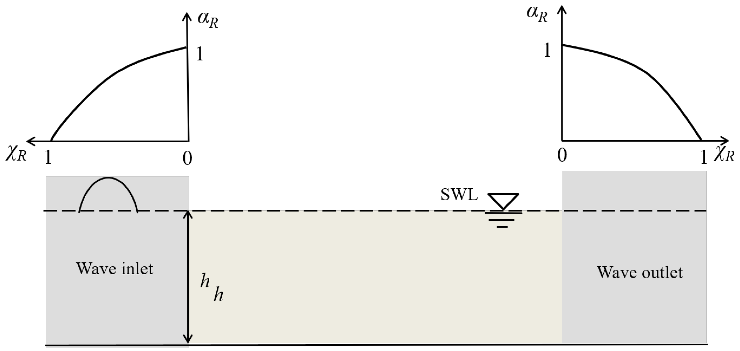
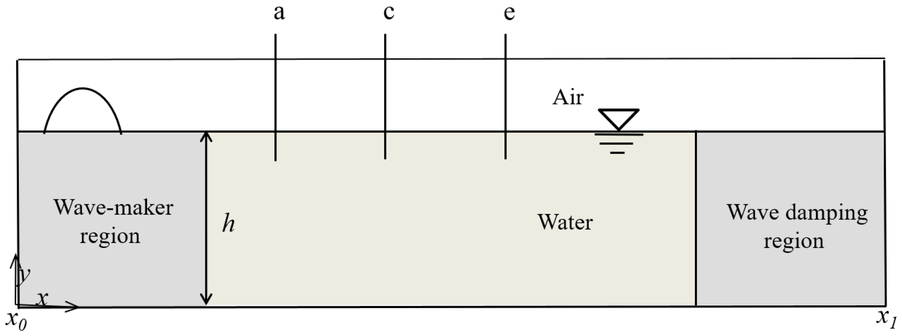
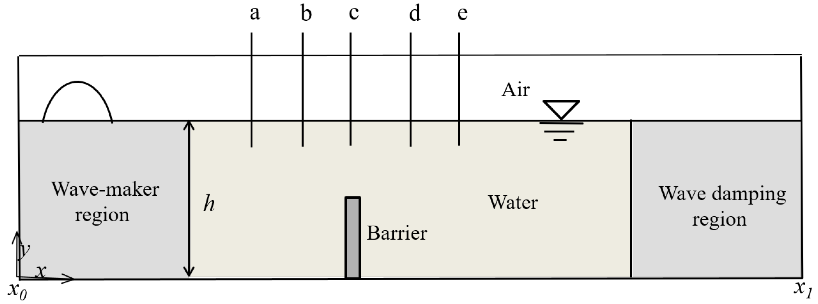
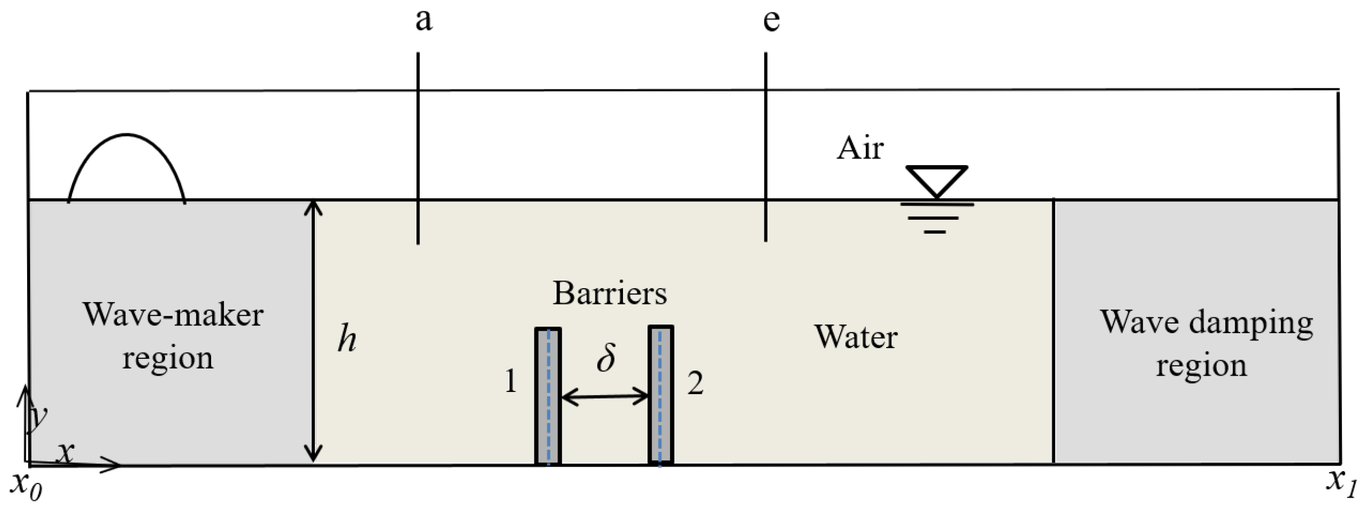
2.3. Wave-Maker with a Relaxation Region

For viscous numerical wave tanks, two kinds of wave makers have been widely used, including the piston wave maker [44,45,46] and the mass source wave maker [47,48]. In order to solve the secondary reflected waves generated during the interaction between solitary waves and structures, a relaxation wavemaker [49] is employed in this study. In the numerical wave tank, the free surface elevation and the velocity components of solitary wave are applied to the entrance boundary to generate a solitary wave. The expressions shown in the research of [14,50] are as follows.
η = H sech 2 3 H 4 h 3 X ,
u = η h g h 1 1 4 η h + h 3 h η 1 3 2 y 2 h 2 d 2 η d X 2 ,
v = y h g h 1 1 2 η h d η d X + 1 3 h 2 1 1 2 y 2 h 2 d 3 η d X 3 ,
where
X = c t τ 2 , c = g ( h + H ) , τ = 2 c 4 h 3 3 H tanh 1 0.999 + H h ,
in which η is the free surface elevation, u denotes the horizontal velocity, and v is the vertical velocity. h is the still-water depth, and H is wave height. c is wave celerity, and 99.9 % of the solitary wave can be generated during the duration τ .
Here, a relaxation zone is implemented at the entrance to correct the solitary waves generated by the wave-maker boundary. By this way, the reflected wave in the computational domain to interfere with the wave-maker boundary could be avoided internally [49]. Another relaxation zone is also set up at the wave outlet to avoid wave reflection from the outlet boundary. The diagram of the wave flume is shown in Figure 1. A relaxation function
α R χ R = 1 exp χ R 3.5 1 exp 1 1 χ R 0 , 1 ,
is applied inside the relaxation zone in the following way,
ψ = α R ψ c o m p u t e d + 1 α R ψ t a r g e t ,
where ψ is either u or ϕ . ψ c o m p u t e d represents the solution of the flow field, and ψ t a r g e t denotes the value we expect. More details about the wave making method could be found in [49].

3. Assessment of the VPM–THINC/QQ

3.1. Comparison between the VPM–THINC/QQ Model and interFoam Solver

In this part, the performance of the VPM–THINC/QQ model in simulating the generation and propagation of solitary waves is compared with the interFoam solver. The setup of the computational domain is shown in Figure 2. The length of the empty wave tank from x 0 to x 1 is 18.0 m, and the height is 0.3 m. The still water depth is h = 0.14 m. A solitary wave with wave height of H = 0.07 m is generated. The wave-maker region with 1.5 m wide is at the leftmost part of the wave tank, and the wave damping region with 2.0 m wide is at the rightmost part of the wave tank. The same grid (grid1) is used in the VPM–THINC/QQ model and interFoam solver. The longitudinal grid is uniform along the wave tank, with a size d x of 0.03 m. The minimum vertical grid d y m i n is 0.003 m. Besides, a finer mesh (grid2) is also used in interFoam solver. The mesh is divided into 1800 grids, evenly distributed in the longitudinal direction, with the smallest vertical grid size d y m i n of 0.002 m. The initial time step is set as Δ t = 0.001 s, which would be automatically updated according to the maximum Courant-Friendrichs-Lewy (CFL) number, 0.5. The monitoring points a, c, and e are placed at x = 6, 8, and 10 m, respectively, to measure the variation of water surface. The total simulation time t t o t a l is 12 s.
The snapshots of solitary wave propagation at different times are shown in Figure 3. The simulated results of the VPM–THINC/QQ model, based on grid 1, are compared with those of the InterFoam solver simulations with grid 1 and grid 2. As shown in Figure 3, it can be seen that, under the same grid size, the wave height of solitary waves using the VPM–THINC/QQ model remains constant with increasing time at the same grid size, while the wave height of solitary waves simulated by interFoam solver decrease along the water tank. The wave height of solitary waves at t = 11 s is 0.721 times of the incident wave height. It indicates that the VPM–THINC/QQ model has the advantage to maintain more waveform than the interFoam solver in the solitary wave propagation process. The time series of solitary waves at three monitoring points are shown in Figure 4. The wave heights at x = 6, 8, and 10 m are 0.833, 0.794, and 0.767 times of the original wave height in interFoam solver, respectively. For the VPM–THINC/QQ model, the computed wave heights agree excellently with the original wave heights, which shows that the VPM–THINC/QQ model can effectively eliminate the numerical consumption and achieve high-fidelity propagation of solitary waves. Grid 2 is also used to simulate the solitary wave in empty wave tank by interFoam solver. From Figure 3 and Figure 4, the solitary wave heights are attenuated to about 0.915 times of the original wave heights at t = 11 s. The attenuation of interFoam solver has been significantly improved due to mesh refinement. Moreover, the wave heights at x = 6, 8, and 10 m become 0.962, 0.957, and 0.954 times the original wave height, respectively. However, there is still numerical dissipation compared with the results obtained by VPM–THINC/QQ model, which even uses coarse mesh (grid1). Obviously, the VPM–THINC/QQ model has high fidelity in simulating solitary waves.

3.2. Verification of the VPM–THINC/QQ Model
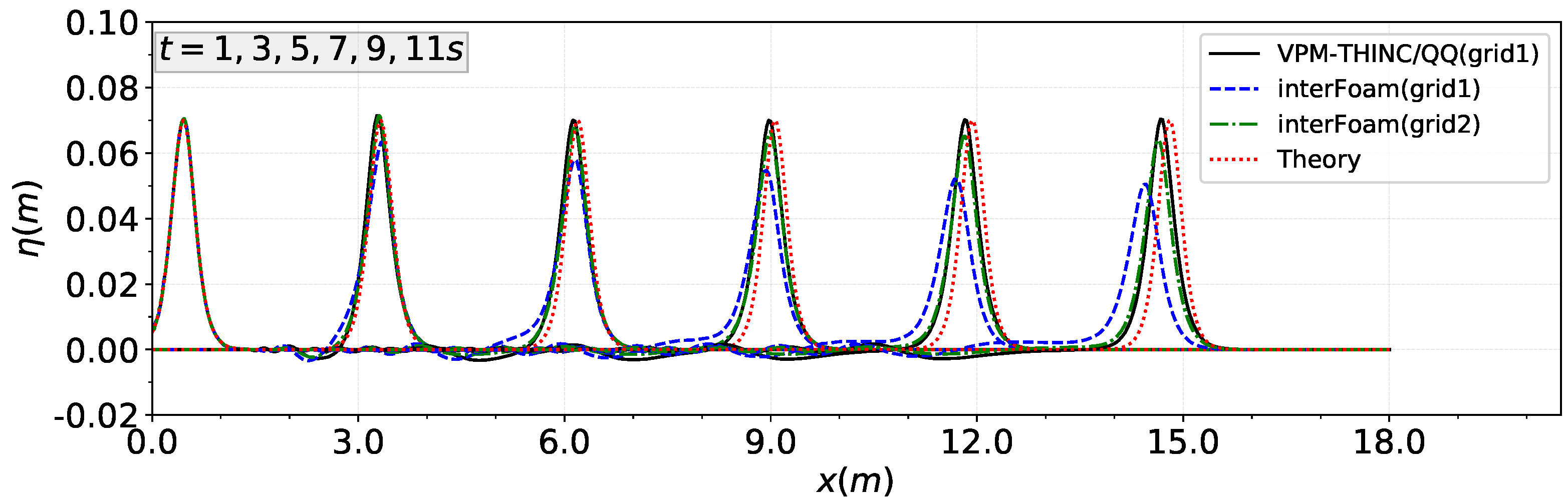
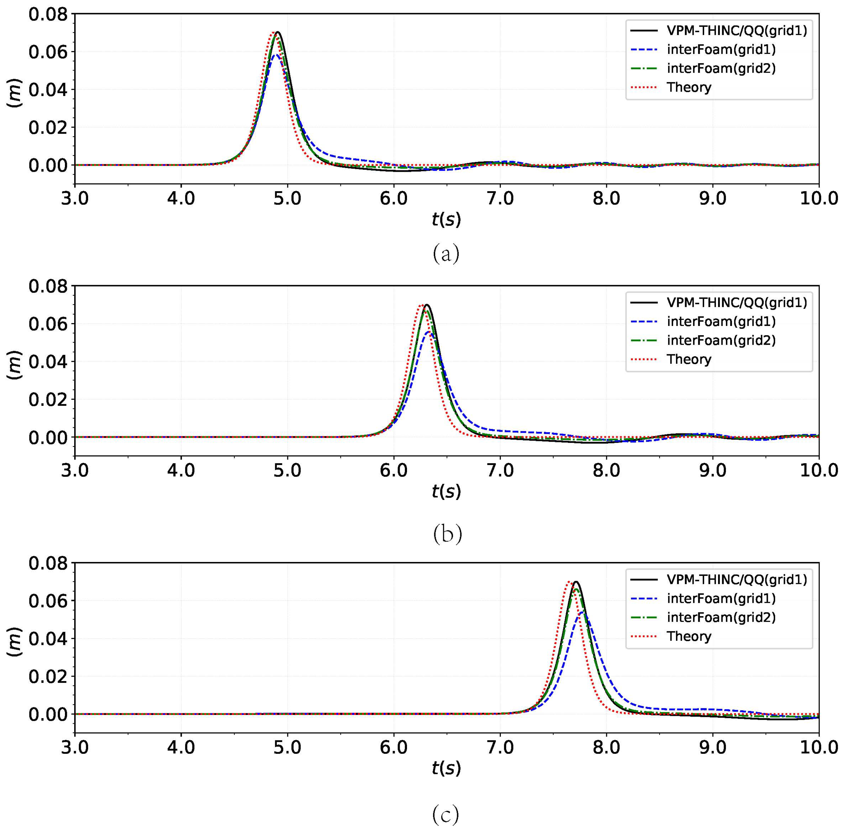
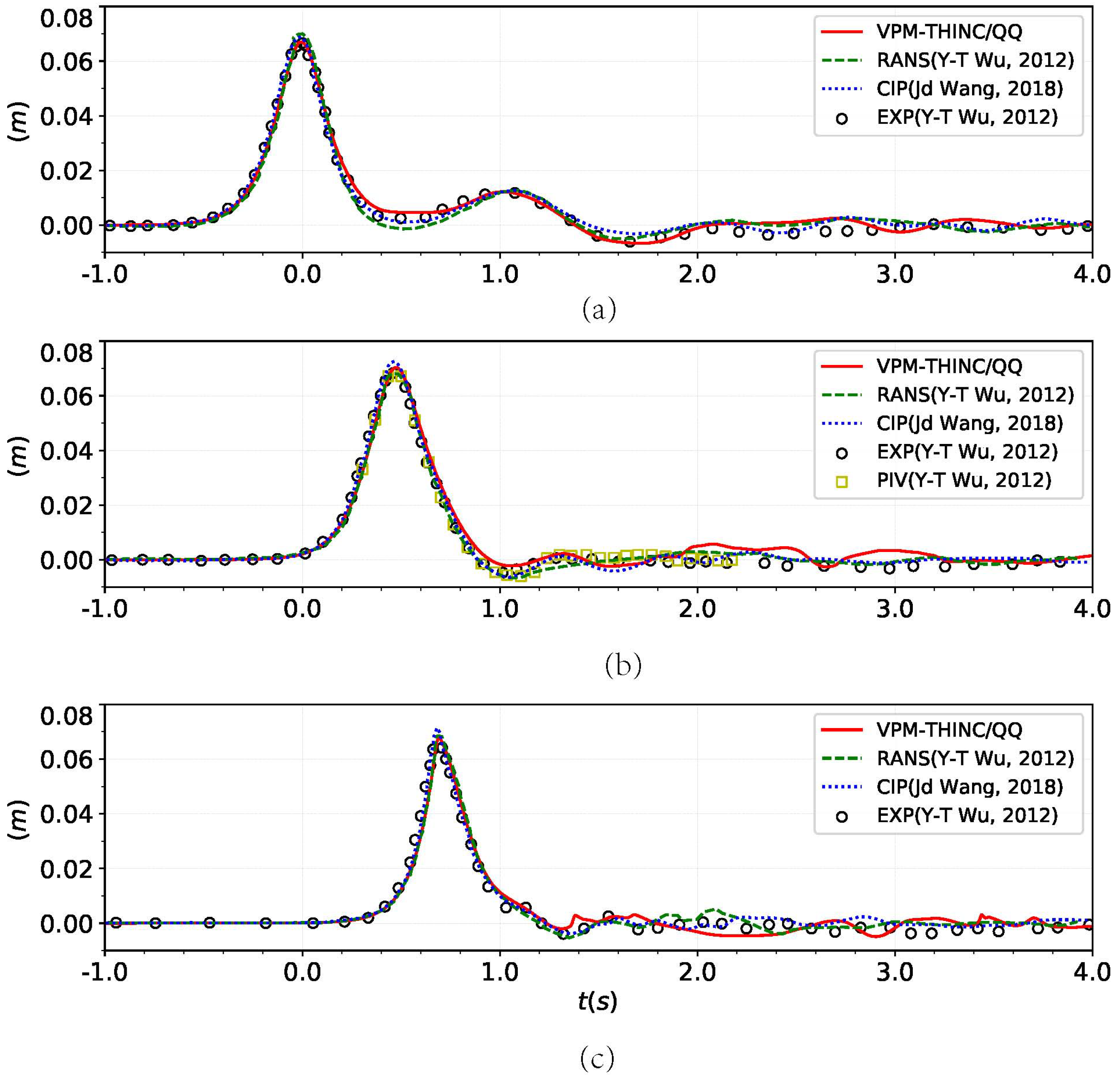
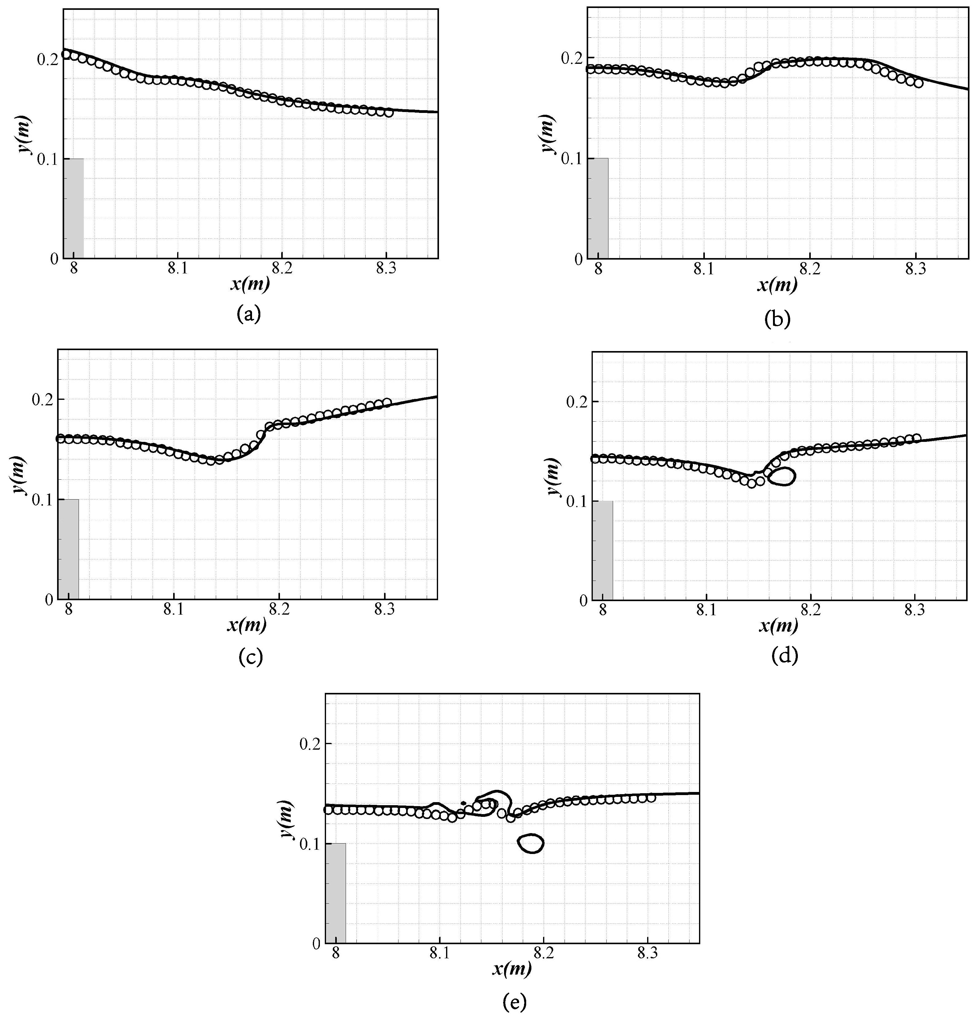
In this part, the performance of the present model in simulating solitary waves, interacting with the underwater barrier, is verified according to the experiment of [39]. The available experimental data and the other numerical results in [39,40] are employed to compare with the results simulated by the present model. The numerical computation domain is shown in Figure 5, which sets the same conditions as Figure 2. The difference is that an underwater barrier is placed in the numerical wave tank. Its central position is at x = 8.0 m, width is W = 0.02 m, and height is d = 0.10 m, respectively. At the same time, five wave monitoring points are placed in the wave flume, and the position of the five wave gauges are at x a = 6.0 m, x b = 7.333 m, x c = 8.0 m, x d = 8.347 m, and x e = 10 m, respectively.
In this case, the solitary wave with wave height of H = 0.07 m is simulated. The free surface variation, the distribution of velocity, and the vortex field are discussed. Following this, the wave forces on the structure subjected to solitary waves with different wave heights are analyzed. In order to expediently compare with the results of [39,40], the time t = 0 s is defined when the crest of the incident wave reaches the position of wave gauge x b .

3.2.1. Free Surface

The time series of free surface variation during solitary wave passing the underwater barrier are shown in Figure 6. The free surface variation in x = 7.333 m, 8.0 m, and 8.347 m are depicted as Figure 6a–c, respectively. The simulated results are compared with the experimental data [39], and the numerical results are simulated by the Reynolds-Averaged Navier–Stokes (RANS) based model [39], as well as the constrained interpolation profile (CIP) based model [40]. From Figure 6, it can be seen that the free surface variation simulated by VPM–THINC/QQ model shows a satisfactory agreement with the experimental measurements and other numerical results on the whole. It should be noted that data observed by particle image velocimetry (PIV) equipment is only plotted in Figure 6b because the view field of PIV system is focused near the underwater barrier. In Figure 6a, the second soliton is clearly observed due to wave reflection. Besides, wave fluctuations caused by wave breaking are found in Figure 6b,c. A similar phenomenon is also observed by [12] when solitary waves pass over the underwater step.
The free surface elevations during solitary wave passing the underwater barrier at t = 0.46, 0.60, 0.74, 0.88, and 1.02 s are shown in Figure 7. The numerical results of the present model (solid line) are compared with the experimental data measured by PIV equipment in [39], which are shown in circle. In Figure 7, it can be seen that the numerical results of the present model keep consistent with PIV’s observations. In their entirety, there are some stages during solitary wave propagating over the underwater barrier, including waves’ “crest-crest exchange”, becoming steep, rolled up, and breaking, respectively. These stages have also been explicitly described in [39,40]. In Figure 7d, some air is entrapped into water, so some water and air mix together (Figure 7e). It is worth mentioning that only one bubble is observed in the present model and the RANS model, which is shown in Figure 7 of [39], while multiple bubbles are observed in Figure 3e of [40]. The explanation for this phenomenon may be that the bubbles burst easily because the surface tension is not taken into account in the CIP-based model. Overall, the present model could simulate the free surface during solitary wave passing the underwater barrier primely in both space and time.

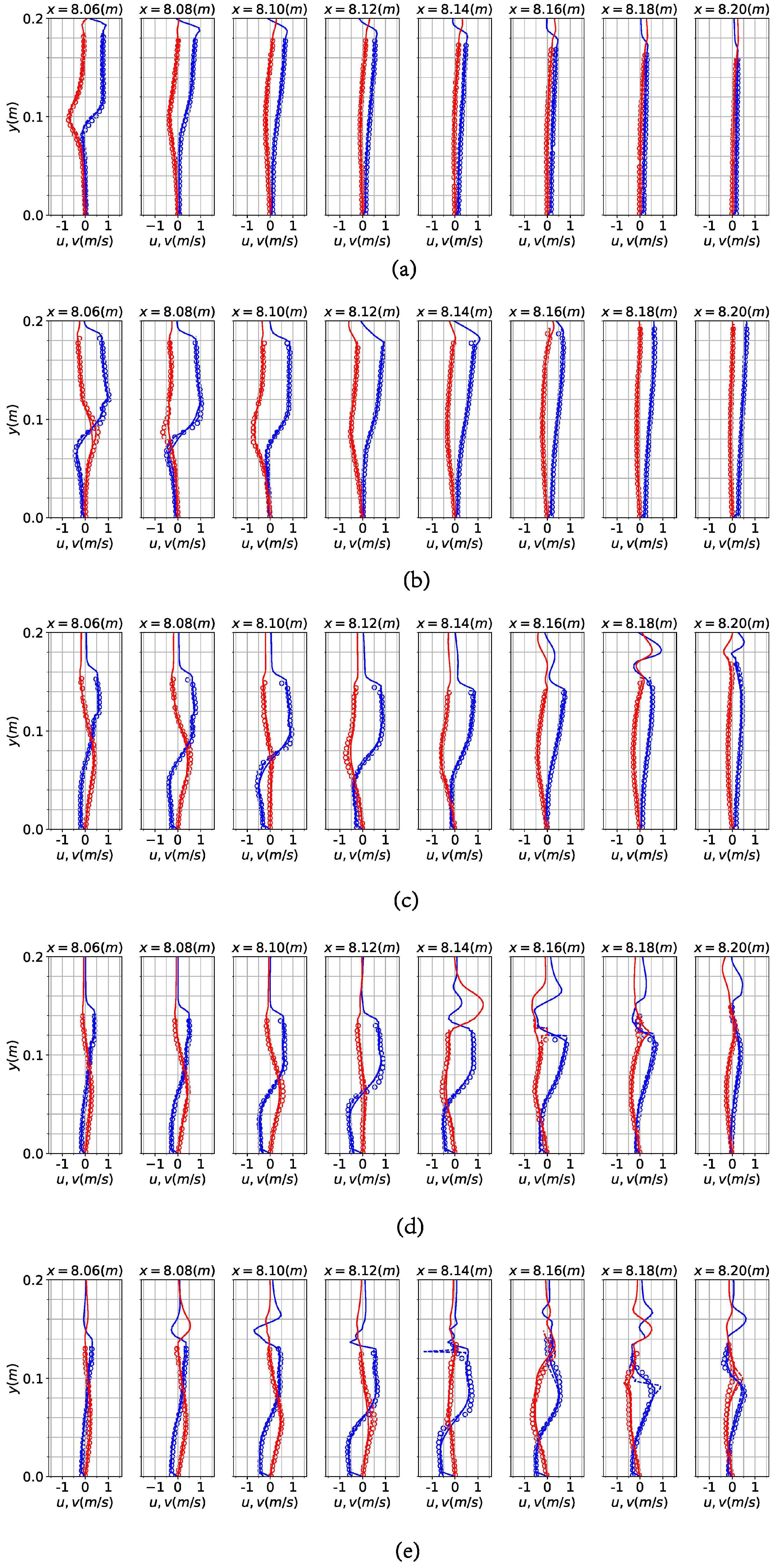
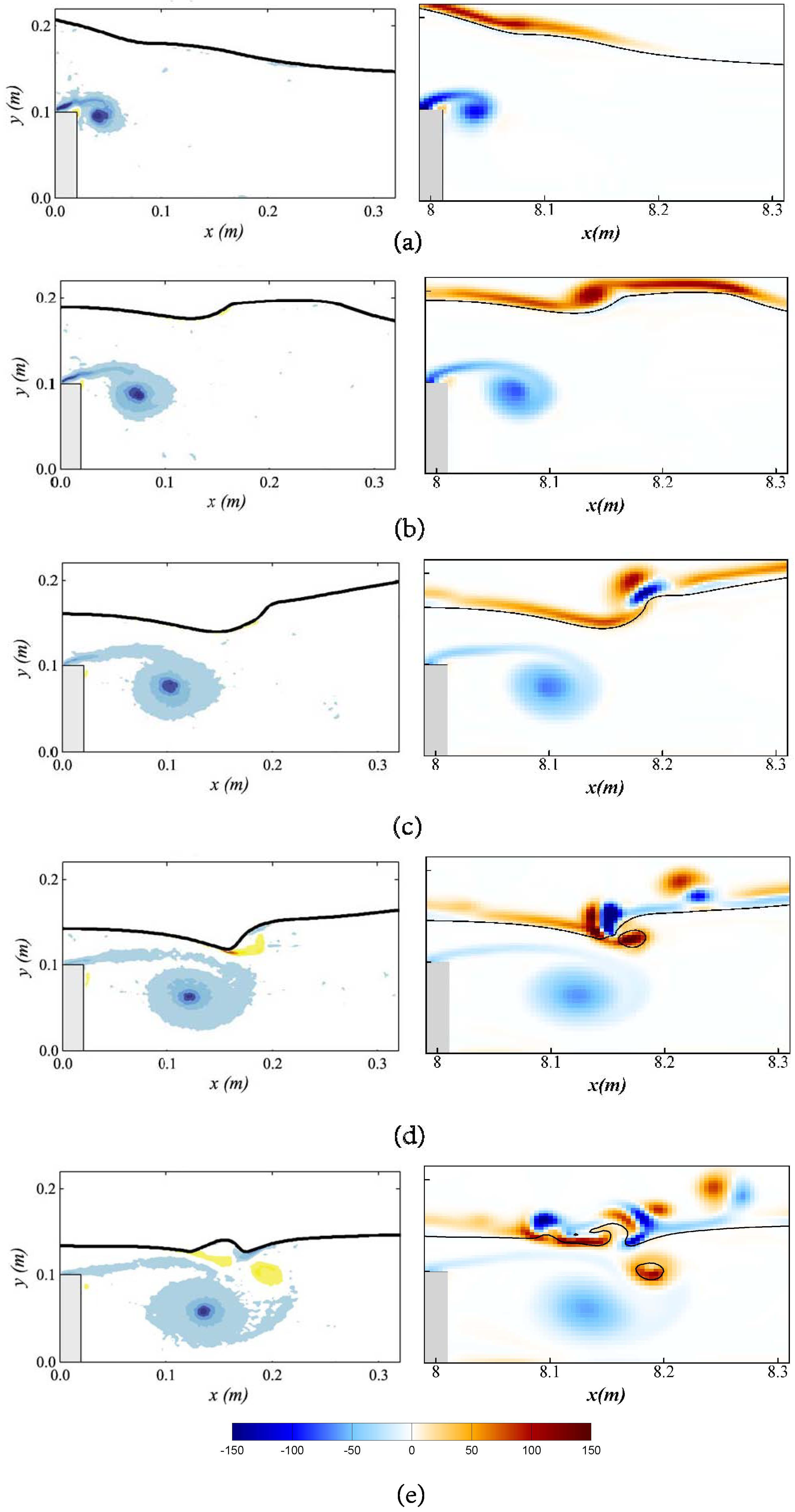
3.2.2. Velocity Distribution and Vorticity Field
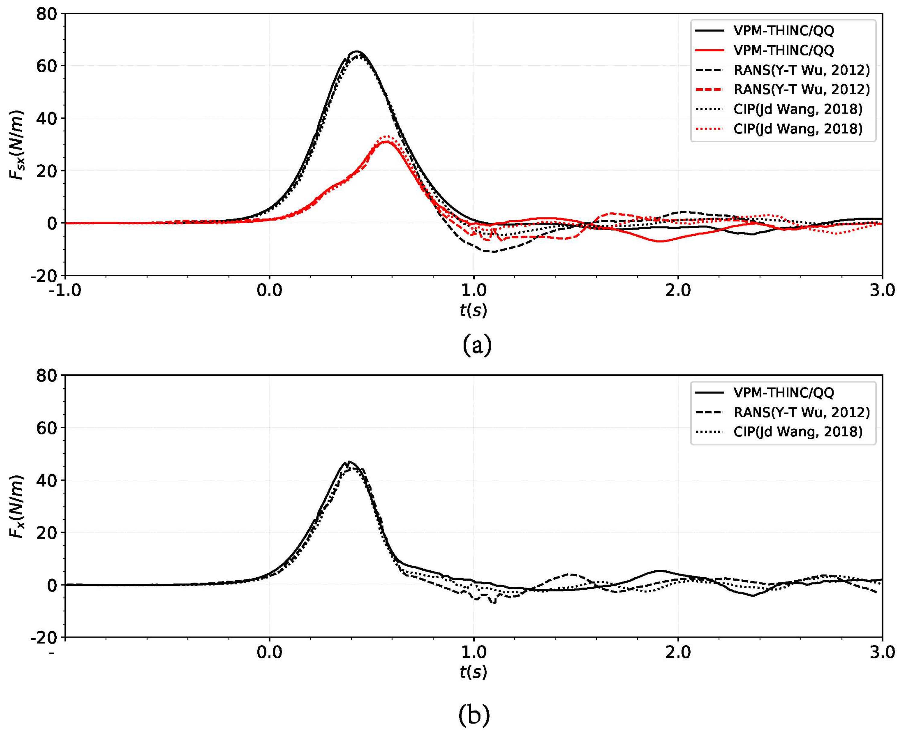
In Figure 8, the velocity distributions at t = 0.46, 0.60, 0.74, 0.88, and 1.02 s are shown as Figure 8a–e, respectively. The velocity profiles from x = 8.06 m to x = 8.20 m, with an identical interval of 0.02m, are depicted. The simulated results are compared with PIV’s measured data, as well as numerical results [39]. From Figure 8, it can be seen that there are velocities above the water surface only found by the present model. The present model is a multiphase flow model in which air is included in fluid calculation. While the RANS model in [39] solves single-phase flow problem and PIV system obtains velocity distributions by monitoring the tracer particles in water, so the air velocity is ignored in both methods. In Figure 8e, the horizontal velocity profile of the present model at x = 8.18 m shows a satisfactory agreement with experimental data, while there are some deviations for the RANS model in [39], expecially at x = 8.14 m and x = 8.18 m. In general, the VPM–THINC/QQ model has an advantage of high accuracy in terms of the velocity distributions.
The vortex generation and evolution during the strong interaction between solitary waves and the underwater barrier are shown in Figure 9. The experimental data of [39] (placed at left) and the VPM–THINC/QQ model results (placed at right) at t = 0.46, 0.60, 0.74, 0.88, and 1.02 s are shown as Figure 9a–e, respectively. The vorticity fields are computed by the operation of ( v / x u / y ). The negative and positive values denote the clockwise and anticlockwise vortices, respectively. From Figure 9a–e, it is obvious that the vorticity fields above the free surface are observed in the present multiphase flow model, but not in experiment [39]. The vorticity fields in air at t = 0.46, 0.60 s are anticlockwise near water surface, but, at t = 0.74, 0.88, and 1.02 s, they appear partly clockwise. The reason for this phenomenon is that water surface begins to move downstream, and the part of the water surface breaks up gradually due to the underwater barrier’s effect. The vortices in water of the present model are basically consistent with the measurements of PIV equipment [39], and the vorticity field of bubble in water is anticlockwise, which also agrees well with the experiment.

3.2.3. Wave forces

The horizontal force acting on the left and right sides of the underwater barrier by solitary waves is shown in Figure 10a. The simulated results are compared with other numerical results computed by the RANS model and the CIP-based model. As shown in Figure 10a, the maximum force on the left side of the barrier is earlier than that on the right side. Meanwhile, the force on the left side is greater than that on the right side. The total horizontal force on the underwater barrier is calculated by subtracting the right force from the left force. The total horizontal force is shown in Figure 10b. In Figure 10, a discrepancy is observed in the tailing stage of the time series due to the complex flow field after wave breaking. In general, the time series of wave forces fit well with other published numerical results.
In order to obtain the universality of the present model, the cases of H / h = 0.1, 0.15, 0.2, 0.35, and 0.5 are simulated by the present model, where H is the solitary wave height, and h is the still water depth. The time series of the total horizontal forces acting on the underwater barrier are plotted in Figure 11a. It can be seen that, for the cases of small wave height, the maximum force appears later because of the low phase velocity. The maximum horizontal forces under different wave heights are compared with that of [39,40], which are shown in Figure 11b. In Figure 11b, the crest of total horizontal force on the barrier increases linearly with the increase in wave height. The phenomenon is also referenced by [51].
In this part, the interaction between solitary waves and the underwater barrier is simulated by the VPM–THINC/QQ model. In terms of the free surface variation, the distribution of velocity, vortex and wave forces, the simulated results of the present model are in good agreement with experimental and other numerical results. On the whole, the ability of the VPM–THINC/QQ model to simulate the interaction between solitary waves and the underwater barrier has been fully verified and assessed.

4. Application of the VPM–THINC/QQ Model

How to effectively reduce wave energy damage is an important issue in coastal protection. From the above study, it can be found that an underwater barrier can consume a portion of the energy of solitary waves to reduce their impact on the coast. In this section, a newly added barrier (see Figure 12) is placed in the downstream of the original barrier in order to achieve more wave energy dissipation. Note that the newly added barrier is the same as the original barrier. The width of the two barrieres are W = 0.02 m, and height are d = 0.10 m, respectively. In Figure 12, δ is the space between the two underwater barriers, h is the still water depth. At the same time, two wave monitoring points, a and e, are placed in the wave flume.
In order to quantitatively study the influence of two underwater barriers on wave energy dissipation, the reflection coefficient, transmission coefficient, and dissipation coefficient of solitary waves are analyzed. Shao [52] defines the coefficient of transmission as C t = H t / H i , reflection as C r = H r / H i , and dissipation as C d = H d / H i , where H t , H r , H d , and H i are the transmitted, reflected, dissipated, and incident wave heights, respectively. As described in [40], the incident wave height H i and the reflected wave height H r correspond to the maximum value and the second largest value of the wave surface at x = 6.0 m, respectively. In addition, the largest value of the wave surface at x = 10.0 m denotes the transmitted wave height H t . In this study, C r , C t , and C d are totally named as the RTD coefficients, and the relationship between them can be established according to energy conservation law in Equation (18). It should be noted that C r and C t are computed by H i , H r , and H t , but C d is obtained according to the energy conservation law.
C t 2 + C r 2 + C d 2 = 1 .
The space between two underwater barriers δ and the wave height of solitary waves H are selected as important parameters for the RTD coefficients to explore the interaction between solitary waves and dual underwater barriers. The space δ = 0.5–6.0 d, with the equal interval of 0.5 d between the two underwater barriers and solitary waves with H / h = 0.1, 0.15, 0.2, 0.35, and 0.5, are chosen for numerical simulation. The total of 60 cases is shown in Table 1, where h is the still water depth, and d is the height of underwater barrier.

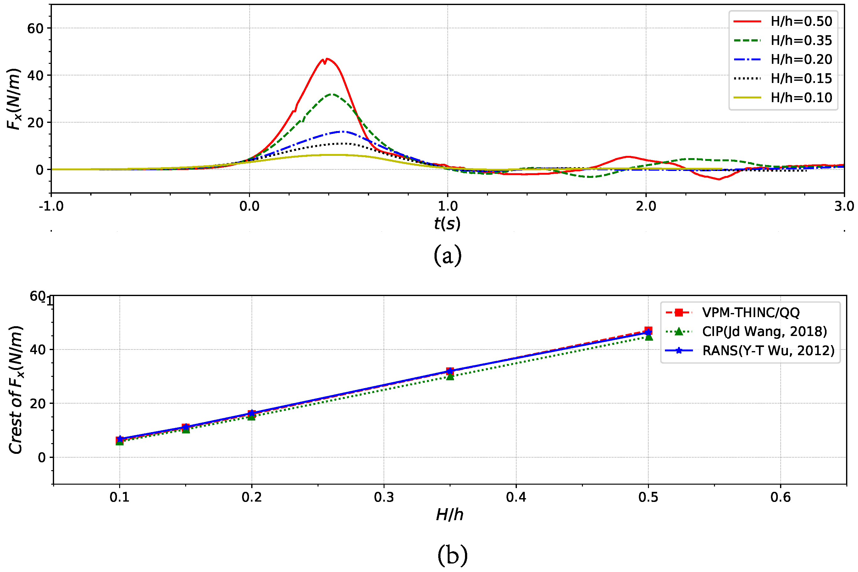
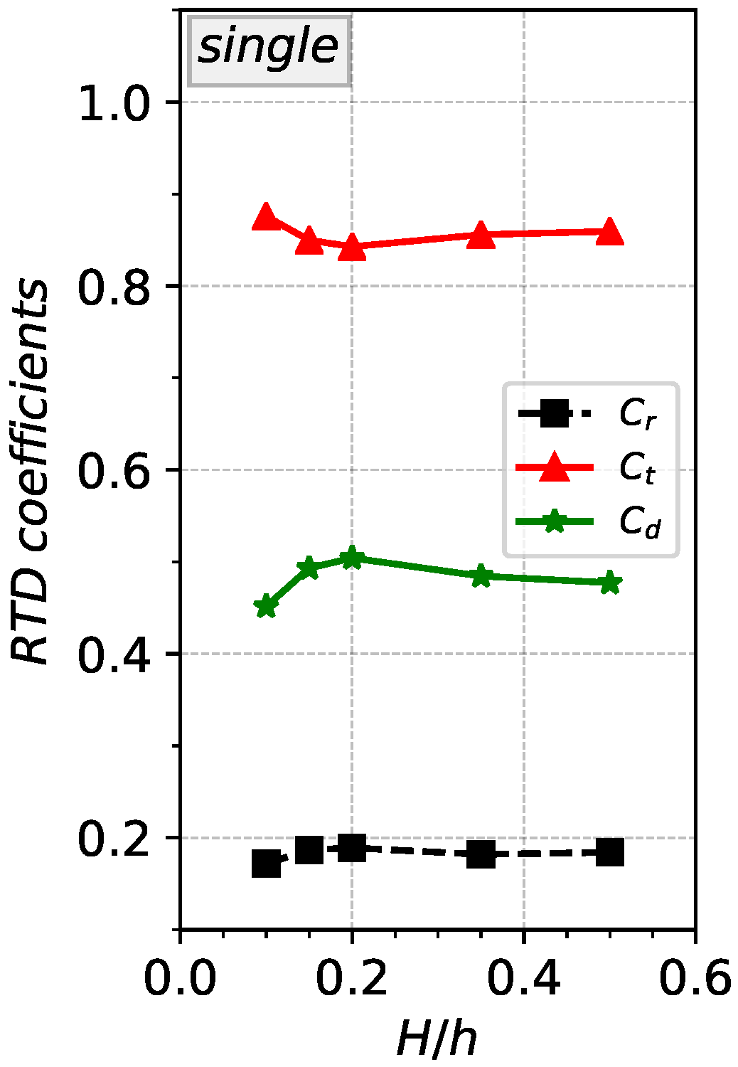
4.1. The RTD Coefficients with Single Underwater Barrier

In Section 3.2, the interaction of solitary waves with a single underwater barrier are simulated by using the VPM–THINC/QQ model. The RTD coefficients during the process of solitary waves passing over a single underwater barrier are calculated and plotted in Figure 13. As shown in Figure 13, the coefficient of wave reflection C r increases with the increase in wave height for values, ranging from 0.10 to 0.20, and then remains basically unchanged. The wave transmission coefficient C t decreases as the wave height increases for values, ranging from 0.10 to 0.20, and then slowly increases for non-linearity values of waves, ranging from 0.20 to 0.50. The trend of wave dissipation coefficient C d is opposite to that of wave transmission coefficient C t . It is worth pointing out that, when the wave height of solitary wave is 0.028 m, the maximum energy dissipation occurs, and the dissipation coefficient is 0.504.

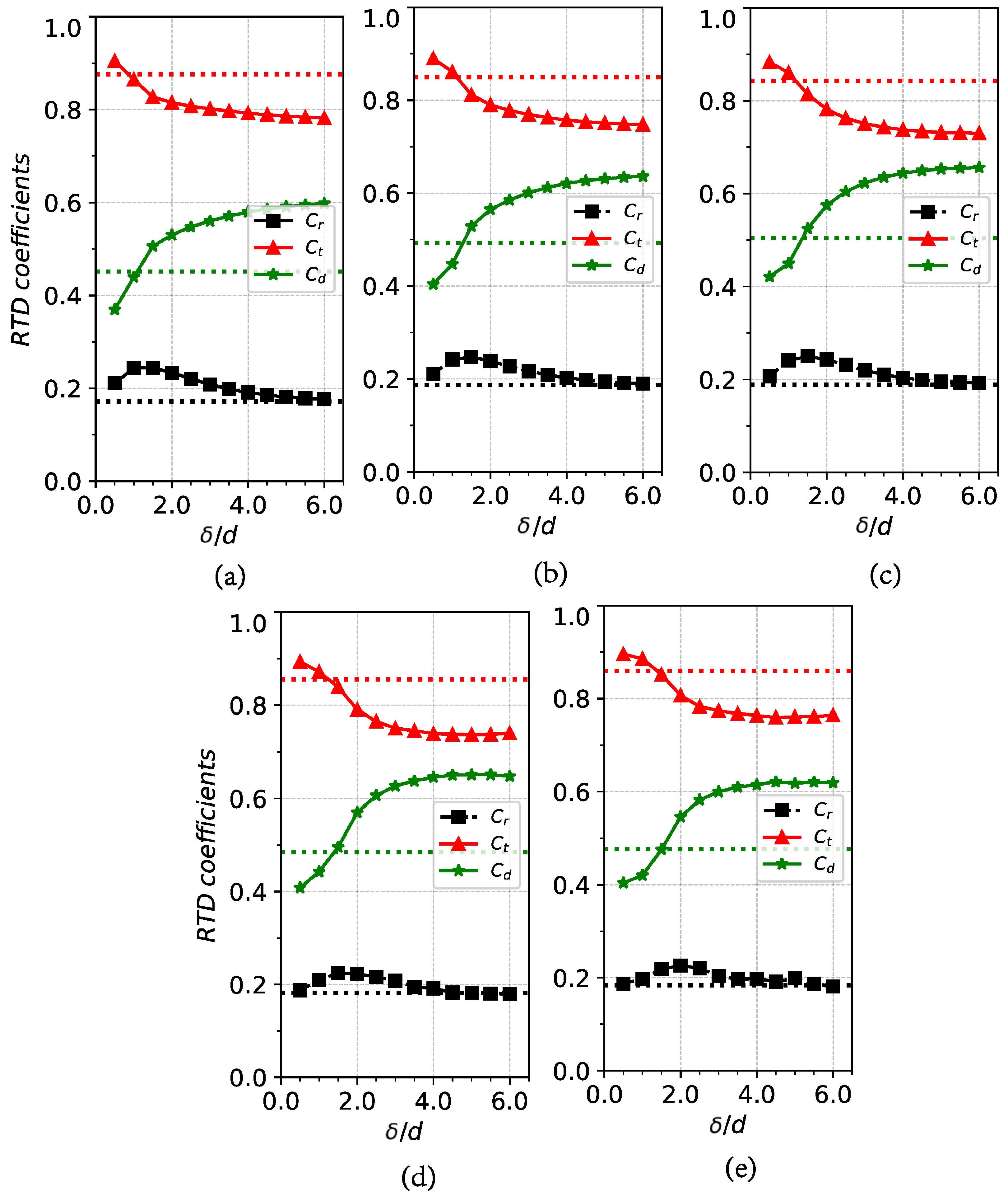
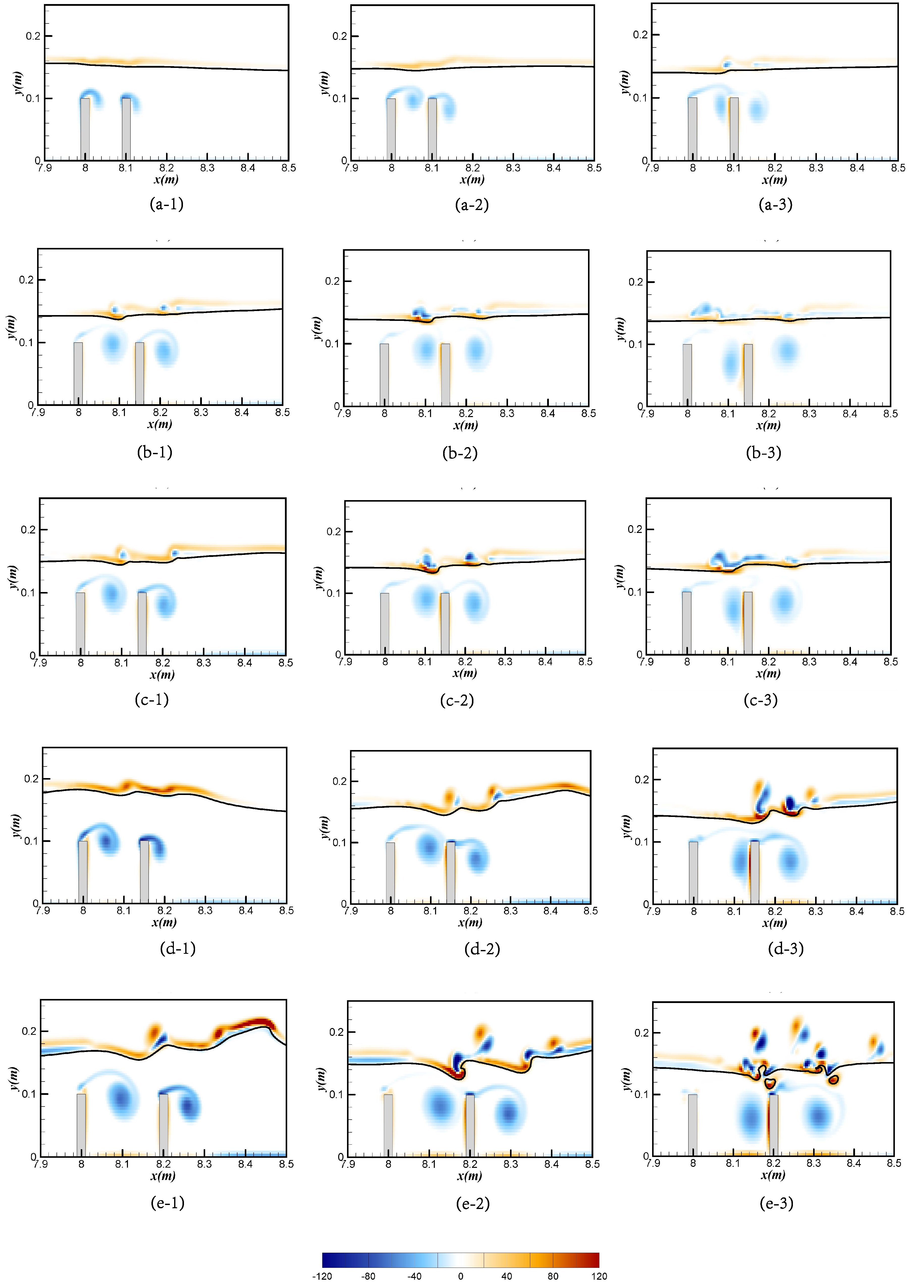
4.2. The RTD Coefficients with Double Underwater Barriers

Figure 14 shows the variation of RTD coefficients during the process of solitary waves interacting with the double underwater barriers. As shown in Figure 14, the changing trends of the RTD coefficients for solitary waves with different wave heights are the same as the cases with different spaces between double underwater barriers in general. The wave reflection coefficient C r increases rapidly and then decreases slowly as the space between two barriers increases.
The coefficient of wave transmission C t decreases monotonously with increasing space between two barriers. The trend of variation in wave dissipation coefficient C d is opposite to that of wave transmission coefficient C t . In Figure 14a, the transmission coefficients of double underwater barriers C t are smaller than that of the single underwater barrier from δ / d = 1.0 to 6.0 for H / h = 0.1. While in Figure 14b–e, the transmission coefficients of double underwater barriers C t are larger than that of single underwater barrier between δ / d = 1.0 and δ / d = 1.5 for H / h = 0.15, 0.2, 0.35, and 0.5. The reason for this phenomenon is that, as the wave height increases, the transmission coefficient of the double underwater barrier requires more space to reach that of a single underwater barrier. As the wave height increases, there needs to be more space to enhance the dissipation capacity of the double underwater barrier compared to a single barrier. When the distance between the double barriers is small, the wave reflection increases. The reflection coefficient occurs at maximum at δ / d = 1.0 for H / h = 0.1 in Figure 14a, but for H / h = 0.5 at δ / d = 2.0 in Figure 14e. This indicates that the higher the wave height, the greater the space between the dual underwater barriers required to achieve maximum wave reflection. As the space between the double submerged barriers increases, the impact of the second barrier on wave reflection is relatively small. For the same wave height, the reflection coefficient gradually becomes the same as that of the single barrier. In Figure 14d, the wave transmission coefficients for H / h = 0.35 is reduced from 0.856 to 0.737 by placing another barrier downstream of the barrier at x = 8.5 m. In Figure 14e, the wave transmission coefficients for H / h = 0.5 is reduced from 0.859 to 0.760 by placing another barrier downstream of the barrier at x = 8.45 m, which could provide a reference for coastal protection.
The vorticity distributions of the maximum reflection coefficient for each wave height are shown in Figure 15. Figure 15a–e depict the H / h = 0.10 and δ / d = 1.0 (case1b), H / h = 0.15 and δ / d = 1.5 (case2c), H / h = 0.20 and δ / d = 1.5 (case3c), H / h = 0.35 and δ / d = 1.5 (case4c), and H / h = 0.5 and δ / d = 2.0 (case5d), respectively. As shown in Figure 15, the vortex shedding from the first barrier is blocked by the second barrier, which causes more reflection of the wave surface. The resulting vortices move between barriers and dissipate energy. As a whole, the higher the wave height, the higher the reverse motion of the wave surface. In Figure 15e, the range of vorticity is large because the maximum wave height has a large amount of energy. The increasing space between double underwater barriers can not effectively form wave surface reflection, so there is less energy reflected back. However, it provides more space for vortices in the water to move and dissipate more energy. As the distance between the two barriers increases, the energy of the wave reflection from the second barrier partially dissipates before reaching the first barrier, and it ultimately completely dissipates. At the same time, the wave dissipation between the barriers reaches saturation and does not generate more dissipation. The transmitted wave energy no longer decreases and tends to stabilize.

5. Conclusions

In this study, an in-house numerical framework (the VPM–THINC/QQ model) of the VPM scheme for solving the flow field and the THINC/QQ method for interface capture is established. The propagation of solitary waves and their interactions with underwater barriers are investigated by the present model. The solitary wave is generated by using a relaxed wave-maker method. The well established interFoam solver is employed to comparatively verify the accuracy and applicability of the present model. With the same coarse grid setting (grid1), the wave height at t = 11 s has become 0.721 times of the original wave height in interFoam solver, while remaining almost unchanged in the present model. Compared to the attenuation phenomenon of the simulation results of the interFoam solver, which cannot be eliminated by encrypting the mesh, the present model is able to simulate the generation and propagation of solitary waves stably and accurately.
The solitary wave passing over a single underwater barrier is simulated and studied based on the present model. Good agreements are obtained by comparing with experimental data and other numerical simulation results in the aspects of the free surface, velocity distribution, vorticity field, and structural forces. All comparisons demonstrate the excellent accuracy of the coupled VPM–THINC/QQ model in predicting the interaction characteristics of solitary waves and underwater barriers.
On the basis of the adequately validated and verified VPM–THINC/QQ coupling numerical model, this paper simulates and studies the effects of dual underwater barriers on the reflection, transmission, and dissipation coefficients of solitary waves. The results show that, as the space between two underwater barriers increases, the reflection coefficient increases first and then decreases, the transmission coefficient decreases monotonously, and the dissipation coefficient is opposite to the transmission coefficient for different wave heights. Moreover, it is found that the wave reflection would be enhanced as the number of underwater barriers increases. Besides, the proper space between the double underwater barriers would play an important role in the generation of vortexes in different directions, which is conducive to the dissipation of wave energy. All the above results indicate that the present model can serve as a powerful tool to simulate the generation and propagation of solitary waves and their interaction with ocean structures. In the future, a large number of numerical cases will be carried out by the present model to simulate the real events in coastal engineering.

Author Contributions

Conceptualisation and methodology, M.L., X.Z. and M.Y.; software, M.L., X.Z. and M.Y.; validation, Y.Z.; writing original draft preparation, M.L.; writing review and editing, M.L., X.Z., J.L., S.Y., G.Q. and H.L.; visualisation, Y.Z.; Supervision, X.Z. and J.L.; funding acquisition, J.L., S.Y., G.Q. and H.L. All authors have read and agreed to the published version of the manuscript.

Funding

This study was financially supported by the fellowship of China Postdoctoral Science Foundation (Grant No. 2021M700540), the Natural Science Foundation of China—Ministry of Water Resources—China Three Gorges Corporation Joint Fund for Changjiang Water Science Research (U2040216), the National Natural Science Foundation of China (Grant Nos. 51979245, 52171247, 42006156), and the Fundamental Research Funds for Central Public Welfare Research Institutes (CKSF2023321/HL, CKSF2021530/HL).

Institutional Review Board Statement

Not applicable.

Informed Consent Statement

Not applicable.

Data Availability Statement

Data are available upon request due to funding restrictions. The data presented in this study are available upon request from the corresponding author. The data are not publicly available due to funding restrictions.

Conflicts of Interest

The authors declare no conflict of interest.

References

  1. Levin, B.W.; Nosov, M.A. Propagation of a Tsunami in the Ocean and Its Interaction with the Coast. In Physics of Tsunamis; Springer: Cham, Switzerland, 2016; pp. 311–358. [Google Scholar] [CrossRef]
  2. Qu, K.; Ren, X.Y.; Kraatz, S. Numerical investigation of tsunami-like wave hydrodynamic characteristics and its comparison with solitary wave. Appl. Ocean Res. 2017, 63, 36–48. [Google Scholar] [CrossRef]
  3. Synolakis, C. The Runup of Solitary Waves. J. Fluid Mech. 1987, 185, 523–545. [Google Scholar] [CrossRef]
  4. Maiti, S.; Sen, D. Computation of solitary waves during propagation and runup on a slope. Ocean Eng. 1999, 55, 1063–1083. [Google Scholar] [CrossRef]
  5. Wu, N.; Hsiao, S.; Chen, H.; Kuai, R.Y.; Qi, M.; Li, J. Numerical study on the propagation of solitary waves in the near-shore. Ocean Eng. 2018, 165, 155–163. [Google Scholar] [CrossRef]
  6. Ying, L.; Fredric, R. Solitary Wave Runup on Plane Slopes. J. Waterw. Port Coast. Ocean Eng. 2001, 127, 33–44. [Google Scholar] [CrossRef]
  7. Liang, D.; Liu, H.; Tang, H.; Rana, R. Comparison Between Boussinesq and Shallow-Water Models in Predicting Solitary Wave Runup on Plane Beaches. Coast. Eng. J. 2013, 55, 1350014-1–1350014-24. [Google Scholar] [CrossRef]
  8. Hsiao, S.; Hsu, T.; Lin, T.; Chang, Y. On the evolution and run-up of breaking solitary waves on a mild sloping beach. Coast. Eng. 2008, 55, 975–988. [Google Scholar] [CrossRef]
  9. Chang, Y.; Hwang, K.; Hwung, H. Large-scale laboratory measurements of solitary wave inundation on a 1:20 slope. Coast. Eng. 2009, 56, 1022–1034. [Google Scholar] [CrossRef]
  10. Smith, L.; Jensen, A.; Pedersen, G. Investigation of breaking and non-breaking solitary waves and measurements of swash zone dynamics on a 5° beach. Coast. Eng. 2017, 120, 38–46. [Google Scholar] [CrossRef]
  11. Kim, S.K.; Liu, P.L.-F.; Liggett, J.A. Boundary integral equation solutions for solitary wave generation, propagation and run-up. Coast. Eng. 1983, 7, 299–317. [Google Scholar] [CrossRef]
  12. Seabra-Santos, F.J.; Renouard, D.P.; Temperville, A.M. Numerical and experimental study of the transformation of a solitary wave over a shelf or isolated obstacle. J. Fluid Mech. 1987, 176, 117–134. [Google Scholar] [CrossRef]
  13. Li, J.; Liu, H.; Gong, K.; Tan, S.K.; Shao, S. SPH modeling of solitary wave fissions over uneven bottoms. Coast. Eng. 2012, 60, 261–275. [Google Scholar] [CrossRef]
  14. Liu, P.L.-F.; Cheng, Y. A numerical study of the evolution of a solitary wave over a shelf. Phys. Fluids 2001, 13, 1160–1667. [Google Scholar] [CrossRef]
  15. Lin, P. A numerical study of solitary wave interaction with rectangular obstacles. Coast. Eng. 2004, 51, 35–51. [Google Scholar] [CrossRef]
  16. Lara, J.L.; Losada, I.J.; Maza, M.; Guanche, R. Breaking solitary wave evolution over a porous underwater step. Coast. Eng. 2011, 58, 837–850. [Google Scholar] [CrossRef]
  17. Wu, Y.; Hsiao, S. Propagation of solitary waves over a submerged permeable breakwater. Coast. Eng. 2013, 81, 1–18. [Google Scholar] [CrossRef]
  18. An, C.K.; Jian, H.T.; Liu, P.L.-F. Vortex generation and evolution in water waves propagating over a submerged rectangular obstacle: Part I. Solitary waves. Coast. Eng. 2001, 44, 13–36. [Google Scholar] [CrossRef]
  19. Zhou, Q.; Zhan, J.M.; Li, Y.S. Numerical Study of Interaction between Solitary Wave and Two Submerged Obstacles in Tandem. J. Coast. Res. 2014, 30, 975–992. [Google Scholar] [CrossRef]
  20. Wang, K.-H.; Wu, T.Y.; Yates, G.T. Three-Dimensional Scattering of Solitary Waves by Vertical Cylinder. J. Waterw. Port Coast. Ocean Eng. 1992, 118, 551–566. [Google Scholar] [CrossRef]
  21. Zhao, M.; Cheng, L.; Teng, B. Numerical simulation of solitary wave scattering by a circular cylinder array. Ocean Eng. 2007, 34, 489–499. [Google Scholar] [CrossRef]
  22. Aristodemo, F.; Tripepi, G.; Meringolo, D.D.; Veltri, P. Solitary wave-induced forces on horizontal circular cylinders: Laboratory experiments and SPH simulations. Coast. Eng. 2017, 129, 17–35. [Google Scholar] [CrossRef]
  23. Ramprasad, S.; Niels, M.; Nadir, A.; Steven, P.; Curtis, S. Large-scale solitary wave simulation with implicit incompressible SPH. J. Ocean Eng. Mar. Energy 2016, 2, 313–329. [Google Scholar] [CrossRef]
  24. Liang, D.; Jian, W.; Shao, S.; Chen, R.; Yang, K. Incompressible SPH simulation of solitary wave interaction with movable seawalls. J. Fluids Struct. 2017, 69, 72–88. [Google Scholar] [CrossRef]
  25. Wroniszewski, P.A.; Verschaeve, J.C.G.; Pedersen, G.K. Benchmarking of Navier–Stokes codes for free surface simulations by means of a solitary wave. Coast. Eng. 2014, 91, 1–17. [Google Scholar] [CrossRef]
  26. Guignard, S.; Marcer, R.; Rey, V.; Kharif, C.; Fraunié, P. Solitary wave breaking on sloping beaches: 2-D two phase flow numerical simulation by SL-VOF method. Eur. J. Mech. B/Fluids 2001, 20, 57–74. [Google Scholar] [CrossRef]
  27. Lo, E.Y.M.; Shao, S. Simulation of near-shore solitary wave mechanics by an incompressible SPH method. Appl. Ocean Res. 2002, 24, 275–286. [Google Scholar] [CrossRef]
  28. Tsung, W.-S.; Hsiao, S.-C.; Lin, T.-C. Numerical simulation of solitary wave run-up and overtopping using Boussinesq-type model. J. Hydrodyn. Ser. B 2012, 24, 899–913. [Google Scholar] [CrossRef]
  29. Stansby, P.K. Solitary wave run up and overtopping by a semi-implicit finite-volume shallow-water Boussinesq model. J. Hydraul. Res. 2003, 41, 639–647. [Google Scholar] [CrossRef]
  30. Farhadi, A.; Ershadi, H.; Emdad, H.; Rad, E.G. Comparative study on the accuracy of solitary wave generations in an ISPH-based numerical wave flume. Appl. Ocean Res. 2016, 54, 115–136. [Google Scholar] [CrossRef]
  31. Ha, T.; Shim, J.; Lin, P.; Cho, Y. Three-dimensional numerical simulation of solitary wave run-up using the IB method. Coast. Eng. 2012, 84, 38–55. [Google Scholar] [CrossRef]
  32. Zelt, J.A. The run-up of nonbreaking and breaking solitary waves. Coast. Eng. 1991, 15, 205–246. [Google Scholar] [CrossRef]
  33. Suraj, D.; Lakshman, A.; Mario, F.T. Evaluating the performance of the two-phase flow solver interFoam. Comput. Sci. Discov. 2012, 5, 014016. [Google Scholar] [CrossRef]
  34. Paulsen, B.T.; Bredmose, H.; Bingham, H.B.; Jacobsen, N.G. Forcing of a bottom-mounted circular cylinder by steep regular water waves at finite depth. J. Fluid Mech. 2014, 755, 1–34. [Google Scholar] [CrossRef]
  35. Xie, B.; Ii, S.; Ikebata, A.; Xiao, F. A multi-moment finite volume method for incompressible Navier–Stokes equations on unstructured grids: Volume-average/point-value formulation. J. Comput. Phys. 2014, 277, 138–162. [Google Scholar] [CrossRef]
  36. Xie, B.; Jin, P.; Xiao, F. An unstructured-grid numerical model for interfacial multiphase fluids based on multi-moment finite volume formulation and THINC method. Int. J. Multiph. Flow 2017, 89, 375–398. [Google Scholar] [CrossRef]
  37. Zhang, Z.; Zhao, X.; Xie, B.; Nie, L. High-fidelity simulation of regular waves based on multi-moment finite volume formulation and THINC method. Appl. Ocean Res. 2019, 87, 81–94. [Google Scholar] [CrossRef]
  38. Xie, B.; Xiao, F. Toward efficient and accurate interface capturing on arbitrary hybrid unstructured grids: The THINC method with quadratic surface representation and Gaussian quadrature. J. Comput. Phys. 2017, 349, 415–440. [Google Scholar] [CrossRef]
  39. Wu, Y.-T.; Hsiao, S.-C.; Huang, Z.-C.; Hwang, K.-S. Propagation of solitary waves over a bottom-mounted barrier. Coast. Eng. 2012, 62, 31–47. [Google Scholar] [CrossRef]
  40. Wang, J.; He, G.; You, R.; Liu, P. Numerical study on interaction of a solitary wave with the submerged obstacle. Ocean Eng. 2018, 158, 1–14. [Google Scholar] [CrossRef]
  41. Prosperetti, A.; Tryggvason, G. Computational Methods For Multiphase Flow; Cambridge University Press: Cambridge, UK, 2009. [Google Scholar]
  42. Smagorinsky, J. General circulation experiments with the primitive equations: I. The basic experiment. Mon. Weather Rev. 1963, 91, 99–164. [Google Scholar] [CrossRef]
  43. Gottlieb, S.; Shu, C. Total Variation Diminishing Runge-Kutta Schemes. Math. Comput. 1998, 67, 73–85. [Google Scholar] [CrossRef]
  44. Wu, N.; Hsiao, S.; Chen, H.; Yang, R. The study on solitary waves generated by a piston-type wave maker. Ocean Eng. 2016, 117, 114–129. [Google Scholar] [CrossRef]
  45. Wu, N.; Tsay, T.; Chen, Y. Generation of stable solitary waves by a piston-type wave maker. Wave Motion 2014, 51, 240–255. [Google Scholar] [CrossRef]
  46. Katell, G.; Eric, B. Accuracy of solitary wave generation by a piston wave maker. J. Hydraul. Res. 2002, 40, 321–331. [Google Scholar] [CrossRef]
  47. Chen, Y.; Hsiao, S. Generation of 3D water waves using mass source wavemaker applied to Navier–Stokes model. Coast. Eng. 2016, 109, 76–95. [Google Scholar] [CrossRef]
  48. Wu, Y.; Hsiao, S. Generation of stable and accurate solitary waves in a viscous numerical wave tank. Ocean Eng. 2018, 167, 102–113. [Google Scholar] [CrossRef]
  49. Niels, J.; David, F.; Jorgen, F. A wave generation toolbox for the open-source CFD library: OpenFoam. Int. J. Numer. Methods Fluids 2012, 70, 1073–1088. [Google Scholar] [CrossRef]
  50. Lee, J.J.; Skjelbreia, J.E.; Raichlen, F. Measurement of velocities in solitary waves. J. Waterw. Port Coast. Ocean Div. 1982, 108, 200–218. [Google Scholar] [CrossRef]
  51. Liu, P.L.-F.; Al-Banaa, K. Solitary wave runup and force on a vertical barrier. J. Fluid Mech. 2004, 505, 225–233. [Google Scholar] [CrossRef]
  52. Shao, S. SPH simulation of solitary wave interaction with a curtain-type breakwater. J. Hydraul. Res. 2005, 43, 366–375. [Google Scholar] [CrossRef]
Figure 1. A sketchof the variation of α R for both inlet and outlet relaxation zones.
Jmse 11 01011 g001
Figure 2. The layout of two-dimensional numerical wave tank without structures.
Jmse 11 01011 g002
Figure 3. The snapshots of solitary wave propagation at t = 1, 3, 5, 7, 9, 11 s.
Jmse 11 01011 g003
Figure 4. The time series of solitary waves at monitoring stations. (a) x = 6.0 m. (b) x = 8.0 m. (c) x = 10.0 m.
Jmse 11 01011 g004
Figure 5. Schematic view of the numerical computational domain with an underwater barrier.
Jmse 11 01011 g005
Figure 6. Comparison of time series of the free surface elevations at three locations between computational results of the VPM–THINC/QQ model and published results. (a) x = 7.333 m. (b) x = 8.0 m. (c) x = 8.347 m.
Jmse 11 01011 g006
Figure 7. Comparison of snapshots between the VPM–THINC/QQ model and experimental data for the free surface elevations at different times (solid lines and circles indicate current predictions and experimental data from [39], respectively). (a) t = 0.46 s. (b) t = 0.60 s. (c) t = 0.74 s. (d) t = 0.88 s. (e) t = 1.02 s.
Jmse 11 01011 g007
Figure 8. Comparison of the velocity profiles at different times. Circles, dotted lines, and solid lines represent the experiment, RANS, and the VPM–THINC/QQ model. (Blue and red indicate horizontal and vertical velocities, respectively). (a) t = 0.46 s. (b) t = 0.60 s. (c) t = 0.74 s. (d) t = 0.88 s. (e) t = 1.02 s.
Jmse 11 01011 g008
Figure 9. Comparison of snapshots between experimental data (left) and the VPM–THINC/QQ model results (right) for the vortex field at different times. (a) t = 0.46 s. (b) t = 0.60 s. (c) t = 0.74 s. (d) t = 0.88 s. (e) t = 1.02 s.
Jmse 11 01011 g009
Figure 10. (a) Comparison of the horizontal wave forces acting on single side of the barrier in the VPM–THINC/QQ model and other numerical results (Data from [39,40]) (Black and red lines denote the left and right side, respectively). (b) Total horizontal wave forces on the underwater barrier.
Jmse 11 01011 g010
Figure 11. (a) Time series of the total horizontal forces acting on the underwater barrier with different wave heights. (b) Comparison of the total horizontal wave forces acting on the barrier between the VPM–THINC/QQ model and other numerical results (Data from [39,40]).
Jmse 11 01011 g011
Figure 12. Schematic diagram of the numerical wave tank for case3.
Jmse 11 01011 g012
Figure 13. The variation of the RTD coefficients with single underwater barrier with different wave heights.
Jmse 11 01011 g013
Figure 14. The variation of the RTD coefficients with different space between double underwater barriers for different H / h . (a) H / h = 0.10. (b) H / h = 0.15. (c) H / h = 0.20. (d) H / h = 0.35. (e) H / h = 0.5.
Jmse 11 01011 g014
Figure 15. Vorticitydistribution in three stages for the interaction between different heights of solitary waves and double underwater barriers, respectively. (a) H / h = 0.10 and δ / d = 1.0 (case1b). (b) H / h = 0.15 and δ / d = 1.5 (case2c). (c) H / h = 0.20 and δ / d = 1.5 (case3c). (d) H / h = 0.35 and δ / d = 1.5 (case4c). (e) H / h = 0.5 and δ / d = 2.0 (case5d).
Jmse 11 01011 g015
Table 1. The characteristics of cases.
Cases H / h = 0.10 H / h = 0.15 H / h = 0.20 H / h = 0.35 H / h = 0.50
δ / d = 0.5case1acase2acase3acase4acase5a
δ / d = 1.0case1bcase2bcase3bcase4bcase5b
δ / d = 1.5case1ccase2ccase3ccase4ccase5c
δ / d = 2.0case1dcase2dcase3dcase4dcase5d
δ / d = 2.5case1ecase2ecase3ecase4ecase5e
δ / d = 3.0case1fcase2fcase3fcase4fcase5f
δ / d = 3.5case1gcase2gcase3gcase4gcase5g
δ / d = 4.0case1hcase2hcase3hcase4hcase5h
δ / d = 4.5case1icase2icase3icase4icase5i
δ / d = 5.0case1jcase2jcase3jcase4jcase5j
δ / d = 5.5case1kcase2kcase3kcase4kcase5k
δ / d = 6.0case1lcase2lcase3lcase4lcase5l
Disclaimer/Publisher’s Note: The statements, opinions and data contained in all publications are solely those of the individual author(s) and contributor(s) and not of MDPI and/or the editor(s). MDPI and/or the editor(s) disclaim responsibility for any injury to people or property resulting from any ideas, methods, instructions or products referred to in the content.

