Efficient Underwater Acoustical Localization Method Based on TDOA with Sensor Position Errors

Abstract

Underwater acoustic localization (UWAL) is extremely challenging due to the multipath nature of extreme underwater environments, the sensor position uncertainty caused by unpredictable ocean currents, and the lack of underwater observation data due to sparse array, which all affect localization performance. Addressing these issues, this paper proposes a simple and effective underwater acoustic localization method using the time difference of arrival (TDOA) measurements based on the multipath channel effect of the underwater environment. By introducing the calibration source, localization performance was improved, and the sensor position error was corrected. The Cramér–Rao lower bound (CRLB) was derived, and the proposed method was able to achieve the CRLB with small deviation. Numerical simulations confirm the improved performance of the proposed method, including (1) a 20 dB and 30 dB reduction in the CRLB for far and near source scenarios, respectively, indicating improved accuracy and reliability when estimating unknown sources; (2) better Mean Squared Error (MSE) performance compared to existing methods and an efficiency of over 90% in low noise and above 80% in moderate noise in several scenarios, with a delayed threshold effect; and (3) achieving CRLB performance with only three sensors in a 3D space, even under moderate noise, while existing methods require at least five sensors for comparable performance. Our results demonstrate the efficacy of the proposed method in enhancing the accuracy and efficiency of source localization.

1. Introduction and Related Works

1.1. Introduction

Underwater acoustic localization (UWAL) has always been the research focus of ocean detection technology, which is widely used in underwater navigation, autonomous underwater vehicle monitoring, and black box searching [1,2,3,4,5,6]. UWAL is a challenging task due to the harsh and dynamic underwater conditions that can affect the accuracy and reliability of the localization system.

The existing UWAL methods are based on the complex Underwater Wireless Sensor Networks (UWSNs) [7]. The modem used for underwater node communication, the deployment of related sensor nodes, and clock synchronization are the key factors for the robustness of UWSNS [8,9]. The selection and deployment of positioning nodes is also a problem that many scholars are constantly exploring [8], and the requirement of clock synchronization in positioning is directly related to the measurement method selected.

This paper considers a common passive acoustic target localization scenario in underwater environments whereby the target emits signals, while sensors with known positions receive the signals. In this scheme, the performance of the localization system is determined by the types of measurements chosen and the positioning algorithm used.

1.2. Related Works

The commonly used measurement types in passive positioning include the received signal strength (RSS) [10,11], angle of arrival (AOA) [12,13], time of arrival (TOA) [14], time difference of arrival (TDOA) [15,16,17,18,19], and frequency difference of arrival (FDOA) [2,20,21] and their combinations [16,21]. Among them, RSS, TOA, and TDOA mainly provide the acoustic propagation time-delay information between the target source and the sensor; AOA and DOA give the angle parameters; and FDOA determines the relative speed between the target and the sensor.

In general, RSS measurements have the advantages of simple calculation and low equipment complexity. However, it becomes quite difficult for sensors to detect and receive the energy of the signal due to the extreme and variable underwater environment; hence, the RSS measurement is rarely considered for underwater acoustic localization. The localization accuracy of TOA heavily relied on clock synchronization between the sensors and the target, which is often not met in practice. Although AOA and DOA have low demand for this, they are not often chosen due to their expensive antenna array and localization systems, which are highly dependent on angular measurement accuracy. FDOA can only be applied to the scene where there is relative motion between the underwater acoustic target and the sensor array, and it is often combined with TDOA. In contrast, TDOA is widely used in target locations due to its low dependence on clock synchronization, high positioning accuracy, and low hardware cost.

The existing localization methods based on TDOA measurements can be divided into three categories, namely the Taylor series expansion method [16,17], the semidefinite programming (SDP) method [22,23], and the least squares (LS) method [24,25,26,27,28]. The Taylor series method is often used in nonlinear equations, and its performance depends heavily on the initial value. If the value is not appropriate, the result may fall into a local optimum. The relaxation transformation of the SDP method is complicated and computationally heavy in practical applications. Without the above disadvantages, LS methods are simple and computationally efficient. The purpose of LS is to convert the nonlinear expression into a linear one by introducing a nuisance variable. The weighted linear LS (WLS), the weighted version of LS, is widely used due to its higher accuracy.

In [24], the classical two-step weighted least square method (TSWLS) is proposed, which considers the constraint relationship between sensor parameters and target position and is easy to calculate. This method can reach the CRLB under a low-noise condition. However, with the increase in noise, the TSWLS algorithm will quickly deviate from the CRLB, resulting in serious estimation errors. In [25], an improved TSWLS method is derived, which directly processed the error term in the second stage, avoided the introduction of pseudolinear equations, and improved positioning accuracy. Nevertheless, this method still does not take into account the problem of sensor position errors in actual TDOA localization. Especially in a complex and changeable underwater environment, it is almost impossible for the sensor to remain stationary due to the influence of unpredictable ocean currents [26]. A TSWLS method for sensor position error is presented in [27]; however, its positioning accuracy was very limited. In [29], a three-step WLS method for sensor position error was developed using a single calibration source, which significantly improved positioning accuracy and could reach the CRLB value under small noise. The above-mentioned literature all assumes that the measurement value of TDOA and its measurement noise are independent of each other. In [30], the correlation between these two parameters is considered, and an iteratively reweighted generalized least squares (IRGLS) method is proposed. Although this method improves localization performance, the complexity of the problem increased to a large degree.

Obviously, none of these methods can directly be used in harsh underwater environments because the actual underwater acoustic channel is complex and the deployment of underwater sensors is sparse, which increases the difficulty of acquiring observation data, resulting in a serious shortage of underwater observation data. Admittedly, a large amount of literature considered these problems. In [28], the authors Gong, Z. et al., proposed a location method based on the angle of arrival using underwater multipath signals, but this method requires a large antenna array with very high cost [28]. Emokpae, L.E. et al., analyzed how Doppler frequency shift affects positioning accuracy in underwater multipath channel positioning [31], Diez-Gonzalez, J. et al., identified direct path signals from underwater multipath signals and positioned underwater targets based on TOA measurement, but this method did not take advantage of the multipath properties of the underwater environment [15]. Thus far, no literature combines underwater multipath nature with the TSWLS method based on TDOA measurement for accurate localization of underwater acoustic sources.

In this paper, we propose a new UWAL solution for the complex underwater environment to further enrich research in this field. The method aims at enhancing underwater positioning accuracy by increasing the number of virtual sensors by exploiting the underwater multipath effect. The proposed approach allows for the localization of a 3D underwater target using only three sensors, leveraging the enriched measurement data of TDOA provided by the multipath effect. An underwater calibration source is introduced to correct the sensor position errors, which can benefit the accuracy of the positioning results. The incorporation of a calibration source also yields more precise sensor location information. An analytical solution based on the least squares method is provided, which requires less computation than the SDP algorithm. The proposed method outperforms iterative algorithms that cannot guarantee a global optimal solution due to improper initial value selection and overcomes the limitations of the minimum number of sensors in traditional TSWLS algorithms.

The rest of this paper is organized as follows. Section 2 presents the underwater localization scenario and an underwater multipath signal model. Section 3 then derives the CRLB corresponding to Section 2. Section 4 develops an efficient underwater multipath (MP) WSL localization algorithm. Section 5 analyzes the theoretical performance of the proposed MP algorithm. Section 6 describes the simulation comparisons, which confirm the effectiveness and accuracy of the proposed method. Finally, Section 7 provides the conclusions.

To provide a quick reference,

Table A1. Parameters and definition.

Parameters	Definition
$s$	Position of the single unknown source
$C$	Position of the calibration source
M	Number of sensors
$R_1$	Position of the reference sensor
$R_{i,0}$	$\mathrm{Position} \mathrm{of} \mathrm{the} \mathrm{receiving} \mathrm{sensors} (i=2,\dots ,M)$
$R_{i,l}$	$\mathrm{Position} \mathrm{of} \mathrm{the} \mathrm{virtual} \mathrm{sensor} (l=0,1,\dots ,L)$
L	Number of multipaths
$R_1{}^{\prime }$	Position of the measured reference sensor
${R^{\prime }}_{i,0}$	Position of the measured receiving sensors
${R^{\prime }}_{i,l}$	Position of the measured virtual sensor
$r_1$	Distance between the sound source and the reference sensor
$r_{i1,l}$	Distance between the sound source and the i-th sensor
$r_i^c$	Distance between the calibration source and the i-th sensor
${\alpha }_{i,l}$	Attenuation coefficient of the $l$-th path
${\mathrm{T}}_{i,l}$	Time delay of the -th path
$w_i(t)$	Noise function of the signal
$s(t)$	Unknown source signal
$C_{i,l}(\tau )$	Cross-correlation function between the signals
$(•{)}^{\ast }$	Complex conjugate of the function
$n_{i1}$	TDOA measurement error
$e_{i1}$	RDOA measurement error
$c$	Sound propagation speed
$r$	$\mathrm{RDOA} \mathrm{measurement} \mathrm{vector}, r={[r_{21,0},r_{21,1},\dots ,r_{21,L},\dots ,r_{M1,L}]}^T$
$e$	$\mathrm{RDOA} \mathrm{measurement} \mathrm{noise} \mathrm{vector}, e=[e_1,e_{2,0},\dots ,e_{2,L},\dots ,e_{M,L}]$
$r^{\prime }$	$r^{\prime }=r+e$
$R$	$\mathrm{Sensor} \mathrm{position} \mathrm{vector}, R=[R_{1,}{R}_{2,0},\dots ,R_{2,L},\dots ,R_{M,L}]$
$w$	$\mathrm{Sensor} \mathrm{position} \mathrm{noise} \mathrm{vector}, w=[w_1,w_{2,0},\dots ,w_{2,L},\dots ,w_{M,L}]$
$R^{\prime }$	$R^{\prime }=R+\omega$
$r^c$	$\mathrm{RDOA} \mathrm{measurement} \mathrm{vector}, r^c={[r_{21,0}^c,r_{21,1}^c,\dots ,r_{21,L}^c,\dots ,r_{M1}^c]}^T$
$n$	$\mathrm{RDOA} \mathrm{measurement} \mathrm{noise} \mathrm{vector}, n=[n_1,n_{2,0},\dots ,n_{2,L},\dots ,n_{M,L}]$
$r^c{}^{\prime }$	$r^c{}^{\prime }=r^c+n$
$Q_{\alpha }$	Covariance matrix of $r^{\prime }$,
$Q_{\beta }$	Covariance matrix of $R^{\prime }$
$Q_c$	Covariance matrix of $r^c{}^{\prime }$
$\mathsf{\theta }$	$\mathrm{Parameter} \mathrm{matrix} \mathrm{of} \mathrm{step} 1 \mathsf{\theta }=[s,R]$
${\epsilon }_c$	RDOA error
$h_c$	Parameter matrix of step 1
$A_c$	Parameter matrix of step 1
$\overline{\omega }$	Sensor position error estimation
$\overline{R^{\prime }}$	Sensors position after calibration
$\Delta \omega$	$\mathrm{Estimation} \mathrm{error} \mathrm{in} \mathrm{step} 1, \Delta \omega =\omega -\overline{\omega }$
${\mathsf{\phi }}_1$	$\mathrm{Unknown} \mathrm{vector} {\mathsf{\phi }}_1={[s^T,{\overline{r}}_1]}^T$
$P_i$	Parameter matrix of step $i$$, i=2 or 3$
$F_i$	Parameter matrix of step $i$$, i=2 or 3$
$h_i$	Parameter matrix of step $i$$, i=2 or 3$
$A_i$	Parameter matrix of step $i$$, i=2 or 3$
${\mathsf{\phi }}_i$	Solution vector of step $i$$, i=2 or 3$
$W_i$	Parameter matrix of step $i$$, i=2 or 3$

in Appendix A summarizes the numerous parameters and their definitions mentioned throughout the paper.

2. Proposed Localization Solution

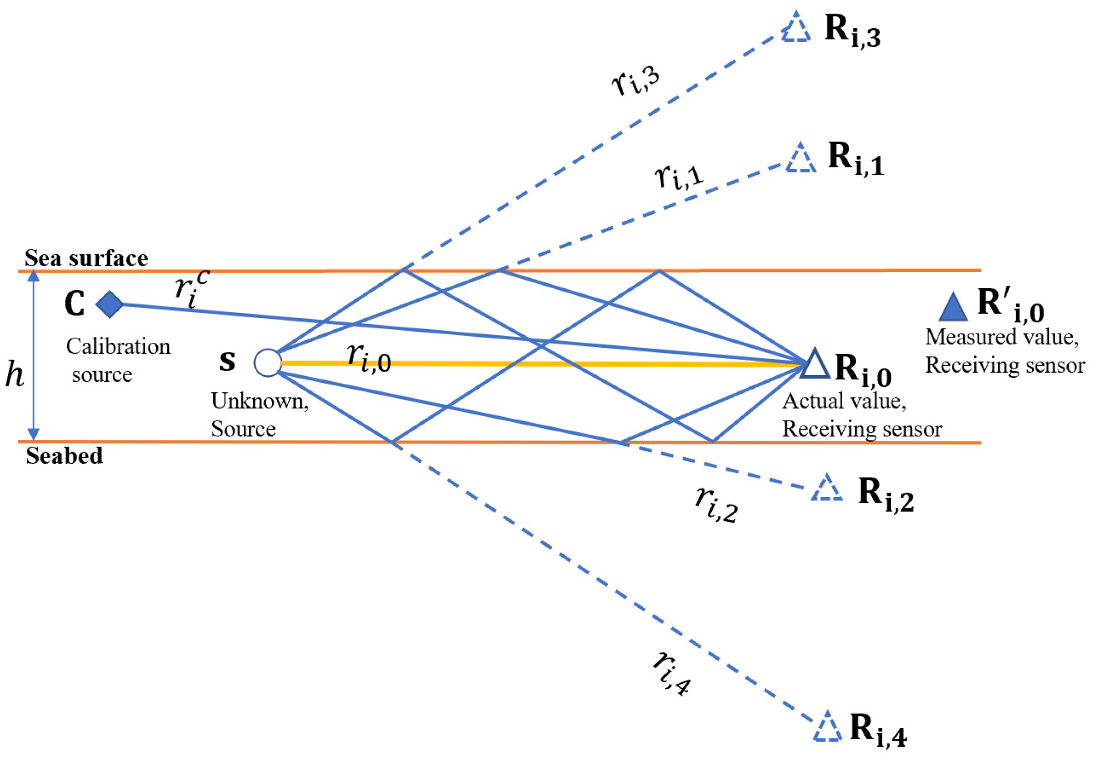
In the real marine environment, the signals transmitted by unknown sources reach the receiving sensors through multiple channels such as linear propagation and sea-surface and seabed reflection.

In theory, the number of multipath signals tends to be infinite, but after multiple reflections, the signal energy loss is often very serious and cannot be detected at the receiving sensor. Moreover, it is not conducive to the extraction of TDOA information; therefore, this paper only considers the primary and secondary reflections. Figure 1 shows the propagation model.

The virtual sensor positions in Figure 1 can be considered as the mirror image of the real sensor positions regarding the sea surface and the seabed.

As shown in Figure 1, a single unknown source is located at $s=[x,y,z]\in {ℝ}^3$, and M receiving sensors are actually located at $R_{i,0}={[x_{i,0},y_{i,0},z_{i,0}]}^T\in {ℝ}^3(i=2,\dots ,M)$, but in practice $R_{i,0}$ is unknown, and we can only obtain the measured value ${R^{\prime }}_{i,0}$ with position error $w_i$. $R_{i,l}={[x_{i,l},y_{i,l},z_{i,l}]}^T\in {ℝ}^3(l=0,1,\dots ,L=4)$ represents the position of the virtual sensor corresponding to the primary and secondary reflections of the sea surface and the seabed, and $r_{i,l}$ denotes the distance between the sound source and the i-th sensor. Similarly, $r_i^c$ is the distance between the calibration source at $C={[x_i^c,y_i^c,z_i^c]}^T$ and the i-th sensor.

In this paper, $R_1$ is used as the reference sensor, only the TDOA that reaches the direct meridian signal is calculated, and the multipath signal is taken at the other receiving sensors.

Assuming that $s(t)$ is an unknown source signal, the multipath signal received by the sensor can be written as

$$f_i(t)={\displaystyle \sum {}_{l=1}^L}{\alpha }_{i,l}s(t-{\mathrm{T}}_{i,l})+w_i(t)$$

(1)

where ${\alpha }_{i,l}$ represents the attenuation coefficient of the $l$-th path, ${\mathrm{T}}_{i,l}$ represents the delay of the $l$-th path, $L$ is the number of multipaths, and $w_i(t)$ represents the noise function. In this paper,$w_i(t)$ is assumed to be zero mean Gaussian white noise and is independent of $s(t)$.

The TDOA value can be obtained by taking the direct path signal ${\alpha }_{l}s(t-{\mathrm{T}}_l)$ in the received signal $f_i(t)$ of the sensor as the reference signal and calculating the cross-correlation between the direct path signal and each multipath signal. The cross-correlation function between the signals is

$$\begin{array}{ll}{C}_{i,l}(\tau )& =E[(f_i(t-\tau ))({\alpha }_{1}s(t-{\mathrm{T}}_1){)}^{\ast }]\\ & ={\alpha }_{i,0}{\alpha }_1^{\ast }{A}_{i,l}(\tau +{\mathrm{T}}_{i,0}-{\mathrm{T}}_1)+{\alpha }_{i,l}{\alpha }_1^{\ast }{A}_{i,l}(\tau +{\mathrm{T}}_{i,l}-{\mathrm{T}}_1)\end{array}$$

(2)

where $E(•)$ and $(•{)}^{\ast }$ represent the expected and complex conjugate of the function, respectively, and A is the autocorrelation function of the signal $s(t)$.

From Equation (2), the measured value of TDOA can be calculated as

$$\Delta {\mathrm{T}}_{i,l}=\arg \max C_{i,l}(\tau )={\mathrm{T}}_{i,l}-{\mathrm{T}}_1+n_{i,l}$$

(3)

where $n_i$ is the TDOA measurement error and $n_i\sim \mathcal{N}(0,{\sigma }_i)$. The corresponding range difference of arrival (RDOA) value is

$$\begin{array}{ll}{r^{\prime }}_{i1,l}& =c\cdot \Delta {\mathrm{T}}_{i,l}=c{\mathrm{T}}_{i,l}-c{\mathrm{T}}_1+c{n}_i\\ & =r_{i,l}-r_1+c{n}_i=r_{i1,l}+e_{i,l}\end{array}$$

(4)

where $c$ indicates the sound propagation speed, $r_{i,l}=‖s_{i,l}-u‖$, $r_1=‖s_1-u‖$, $‖•‖$ is the Euclidean distance norm, and $e_i$ denotes the RDOA measurement error.

3. Cramér–Rao Lower Bound

The Cramér–Rao lower bound (CRLB) is usually used to study the best estimation accuracy that can be obtained in unbiased estimation, so the performance of parameter estimation methods can be evaluated by whether it is close to the CRLB. In this section, we first derive the optimal theoretical performance bound, namely the CRLB, of the location problem in this paper, derive the error covariance matrix of the proposed algorithm, and then analyze and compare them.

For simplicity, several parameters can be rewritten into the matrix form

$$r^{\prime }=r+e$$

(5)

where $r^{\prime }={[{r^{\prime }}_{21,0},{r^{\prime }}_{21,1},\dots ,{r^{\prime }}_{21,L},\dots ,{r^{\prime }}_{M1,L}]}^T$, $r={[r_{21,0},r_{21,1},\dots ,r_{21,L},\dots ,r_{M1,L}]}^T$, $e=[e_1,e_{2,0},\dots ,e_{2,L},\dots ,e_{M,L}]$, and $r^{\prime }\sim \mathcal{N}\left(r,Q_{\alpha }\right)$.

$$R^{\prime }=R+\omega$$

(6)

where $R^{\prime }=[{R^{\prime }}_{1,}{R^{\prime }}_{2,0},\dots ,{R^{\prime }}_{2,L},\dots ,{R^{\prime }}_{M,L}]$, $R=[R_{1,}{R}_{2,0},\dots ,R_{2,L},\dots ,R_{M,L}]$, $w=[w_1,w_{2,0},\dots ,w_{2,L},\dots ,w_{M,L}]$, and $R^{\prime }\sim \mathcal{N}\left(R,Q_{\beta }\right)$.

$$r_{i1,l}^c=r_{i,l}^c-r_1^c=‖C-R_{i,l}‖-‖C-R_1‖(i=2,3,\dots ,M;l=0,1,\dots ,L)$$

(7)

$$r^c{}^{\prime }=r^c+n$$

(8)

where $r^c{}^{\prime }={[r_{21,0}^c{}^{\prime },r_{21,1}^c{}^{\prime },\dots ,r_{21,L}^c{}^{\prime },\dots ,r_{M1}^c{}^{\prime }]}^T$, $r^c={[r_{21,0}^c,r_{21,1}^c,\dots ,r_{21,L}^c,\dots ,r_{M1}^c]}^T$,$n=[n_1,n_{2,0},\dots ,n_{2,L},\dots ,n_{M,L}]$, and $r^c{}^{\prime }\sim \mathcal{N}\left(r,Q_c\right)$.

Let the parameter vector be $\mathsf{\theta }=[s,R]$, $\zeta =[r^{\prime },R^{\prime },r^c{}^{\prime }]$. Since $r^c$, $R^{\prime }$, and $r^c{}^{\prime }$ are Gaussian-distributed and independent of each other, we can express the log-likelihood function of the joint probability density function of the location scenario in Section 3 as

$$\begin{array}{ll}\mathrm{lnP}(\xi ;\theta )& =\mathrm{lnP}(r^{\prime }\left|r\right.;Q_{\alpha })+\mathrm{lnP}(R^{\prime }\left|R\right.;Q_{\beta })+\mathrm{lnP}(r^c{}^{\prime }\left|r^{\prime }\right.;Q_c)\\ & =K-\frac{1}{2}(r^{\prime }-r{)}^T{Q}_{\alpha }^{-1}(r^{\prime }-r)\\ & \hspace{0.33em}\hspace{0.33em}\hspace{0.17em}\hspace{0.17em} -\frac{1}{2}(R^{\prime }-R{)}^T{Q}_{\beta }^{-1}(R^{\prime }-R)\\ & \hspace{0.33em}\hspace{0.33em}\hspace{0.17em}\hspace{0.17em} -\frac{1}{2}(r^c{}^{\prime }-r^c{)}^T{Q}_{\alpha }^{-1}(r^c{}^{\prime }-r^c)\end{array}$$

(9)

where $K$ is a constant independent of unknown parameters.

In the localization scenario of this paper, the CRLB can be expressed as

$$\mathrm{CRLB}(\mathsf{\theta })=\mathrm{I}{(\mathsf{\theta })}^{-1}$$

(10)

The Fisher information matrix $\mathrm{I}(\mathsf{\theta })$ is given as

$$\mathrm{I}(\mathsf{\theta })=\left[\begin{array}{cc}{X}_{11}& X_{12}\\ X_{21}& X_{22}\end{array}\right]$$

(11)

$$\begin{array}{ll}{X}_{11}& =-\mathrm{E}\left[\frac{\partial \mathrm{lnP}(\xi ;\mathsf{\theta })}{\partial s\partial s^T}\right]=(\frac{\partial r}{\partial s}{)}^T{Q}_{\alpha }^{-1}(\frac{\partial r}{\partial s})\\ X_{12}& =-\mathrm{E}\left[\frac{\partial \mathrm{lnP}(\xi ;\mathsf{\theta })}{\partial s\partial R^T}\right]=(\frac{\partial r}{\partial s}{)}^T{Q}_{\alpha }^{-1}(\frac{\partial r}{\partial R})\\ X_{21}& =X_{12}^T\\ X_{22}& =-\mathrm{E}\left[\frac{\partial \mathrm{lnP}(\xi ;\mathsf{\theta })}{\partial R\partial R^T}\right]\\ & =(\frac{\partial r}{\partial R}{)}^T{Q}_{\alpha }^{-1}(\frac{\partial r}{\partial R})+Q_{\beta }^{-1}+(\frac{\partial r^c}{\partial R}{)}^T{Q}_c^{-1}(\frac{\partial r^c}{\partial R})\end{array}$$

(12)

The partial derivatives are given as

$$\frac{\partial r_{i1,l}}{\partial s}=\left[\frac{(s-R_{i,l})}{‖s-R_{i,l}‖}-\frac{(s-R_1)}{‖s-R_1‖}\right]$$

(13)

where $\frac{\partial r_{i1,l}}{\partial s}$ is the $(i-1)$ row of $\frac{\partial r}{\partial s}$,$i=2,3,\dots ,M$;

$$\frac{\partial r_{i1,l}}{\partial R}=\left[{\frac{(s-R_1)}{‖s-R_1‖}}^T,0_{1\times [3(i-2)\cdot (L+1)]}^T,-{\frac{(s-R_{i,l})}{‖s-R_{i,l}‖}}^T,0_{1\times [3(M-i)\cdot (L+1)]}^T\right]$$

(14)

where $\frac{\partial r_{i1,l}}{\partial R}$ is the $(i-1)$ row of $\frac{\partial r}{\partial R}$,$i=2,3,\dots ,M;l=0,1,\dots ,L$; and

$$\frac{\partial r_{i1}^c}{\partial R}=\left[{\frac{(C-R_1)}{‖C-R_1‖}}^T,0_{1\times [3(i-2)\cdot (L+1)]}^T,-{\frac{(C-R_{i,l})}{‖C-R_{i,l}‖}}^T,0_{1\times [3(M-i)\cdot (L+1)]}^T\right]$$

(15)

where $\frac{\partial r_{i1}^c}{\partial R}$ is the $(i-1)$ row of $\frac{\partial r^c}{\partial R}$,$i=2,3,\dots ,M;l=0,1,\dots ,L$.

Finally, we can obtain

$$\mathrm{CRLB}(s^{\prime })={[I\left(1:3,1:3\right)]}^{-1}$$

(16)

4. Proposed Localization Solution

In this section, a closed-form localization algorithm is derived using underwater multipath signals combined with a single calibration source. Compared with the traditional nonmultipath iterative method, this method greatly improves the localization performance of the algorithm by adding virtual array elements, reduces the amount of calculation, avoids the divergence of the algorithm or falling into the local optimal solution caused by the inappropriate initial value, and reaches CRLB accuracy when the noise is relatively small.

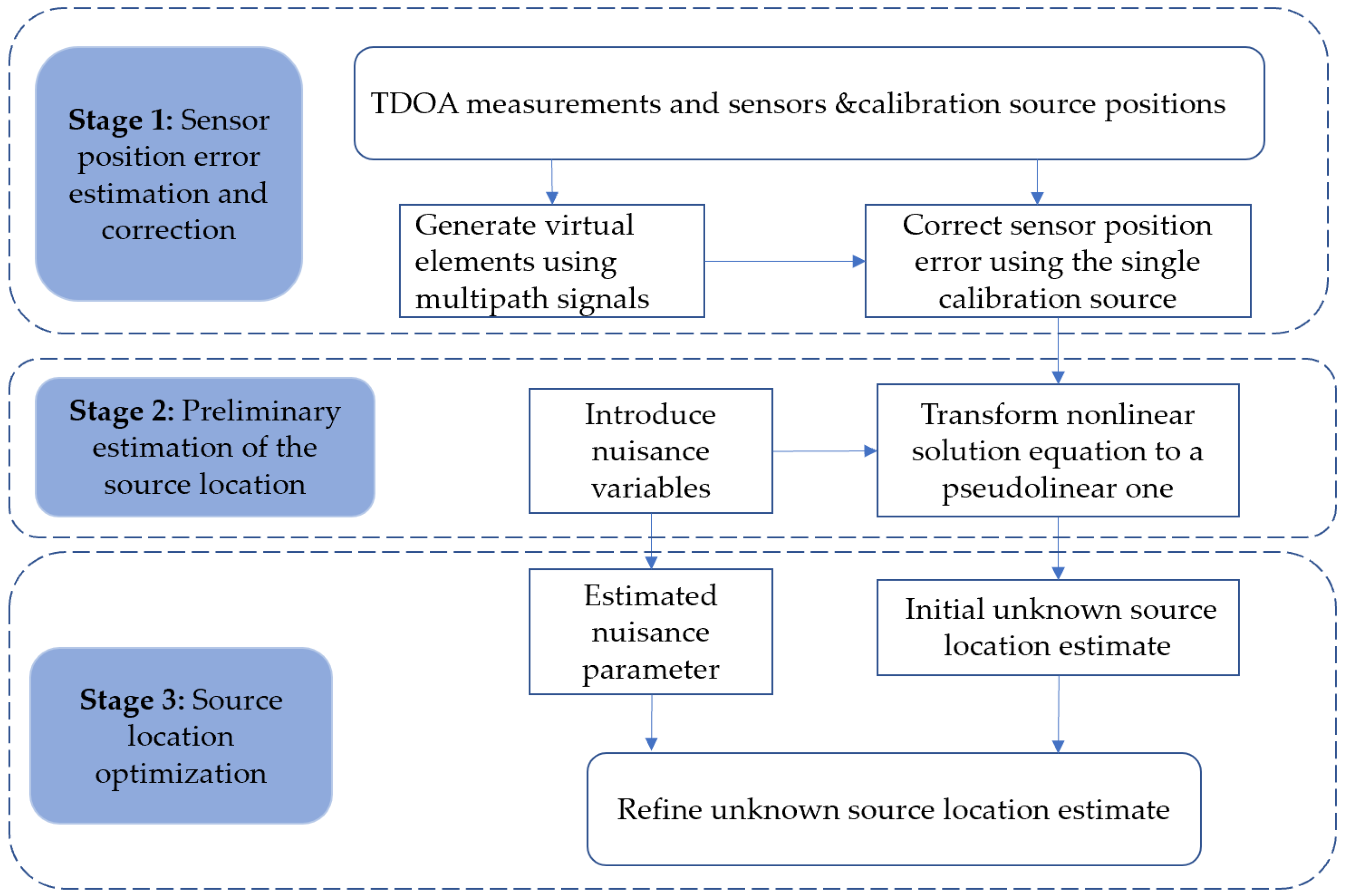
The method proposed in this paper solves the nonlinear localization problem using the following three steps. First, the number of virtual sensors is increased through the introduction of multipath signals, and the sensor position error is corrected by the calibration source. Second, the nuisance variables are introduced to transform the nonlinear equations into pseudolinear equations for the solution. Finally, the estimation position of the unknown source is further optimized by improving the estimation accuracy of the interference variable. The implementation process of unknown source localization is shown in Figure 2.

Step 1: Sensor position error estimation and correction

In the localization case of this paper, the measured sensors are located at $R_1{}^{\prime }$ and ${R^{\prime }}_{i,0}(i=2,\dots ,M)$, and their corresponding virtual sensors that pass the primary and secondary reflections of the sea surface and the seabed are located at ${R^{\prime }}_{i,1}=(x_i,y_i,2h-z_i)$, ${R^{\prime }}_{i,2}=(x_i,y_i,-z_i)$, ${R^{\prime }}_{i,3}=(x_i,y_i,2h+z_i)$, and ${R^{\prime }}_{i,4}=(x_i,y_i,-2h+z_i)$, respectively.

Combining Equations (7) and (8) above, we arrive at

$$r_{i1,l}^{c^{\prime }}=‖C-R_{i,l}‖-‖C-R_1‖+{\mathrm{n}}_{i,l}(i=2,3,\dots ,M;l=0,1,\dots ,L)$$

(17)

In this paper, the true position $R_{i,l}$ of the sensors is unknown, and we can only obtain ${R^{\prime }}_{i,L}$ with the position error. For the above highly nonlinear function of the unknown, let us linearize $‖C-R_{i,l}‖$ and $‖C-R_1‖$ by using the Taylor series expansion up to the linear term

$$\begin{array}{ll}{r}_{i1,l}^{c^{\prime }}& =‖C-{R^{\prime }}_{i,l}+{\omega }_{i,l}‖-‖C-{R^{\prime }}_1+{\omega }_1‖+n_{i,l}\\ & =‖C-{R^{\prime }}_{i,l}‖+\frac{(C-{R^{\prime }}_{i,l})}{‖C-{R^{\prime }}_{i,l}‖}{\omega }_{i,l}-(‖C-{R^{\prime }}_1‖+\frac{(C-{R^{\prime }}_1)}{‖C-{R^{\prime }}_1‖}{\omega }_1)+n_{i,l}\end{array}$$

(18)

The RDOA error ${\epsilon }_c$ caused by sensor position error can be expressed as

$$\begin{array}{c}{\epsilon }_c=r_{i1,l}^c{}^{\prime }-(‖C-{R^{\prime }}_{i,l}‖-‖C-{R^{\prime }}_1‖)\\ =\frac{(C-{R^{\prime }}_{i,l})}{‖C-{R^{\prime }}_{i,l}‖}{\omega }_{i,l}-\frac{(C-{R^{\prime }}_1)}{‖C-{R^{\prime }}_1‖}{\omega }_1+n_{i,l}\end{array}$$

(19)

Equation (19) can be rewritten in a matrix form as

$$h_c=A_c\omega +n$$

(20)

where on the right side is

$$\begin{array}{r}{A}_c[j,:]=[-\frac{(C-{R^{\prime }}_1)}{‖C-{R^{\prime }}_1‖},0_{1\times 3(i-2)\cdot L}^T,\frac{(C-{R^{\prime }}_{i,l})}{‖C-{R^{\prime }}_{i,l}‖},0_{1\times 3(M-2)\cdot L}^T]\\ (j=(i-2)L+(l+1))\end{array}$$

(21)

and on the left side is

$$h_c=\left[\begin{array}{c}{r}_{21,0}^{c\prime }-(‖C-{R^{\prime }}_{2,0}‖-‖C-{R^{\prime }}_1‖)\\ \begin{array}{c}\dots \\ \begin{array}{c}{r}_{21,L}^{c\prime }-(‖C-{R^{\prime }}_{2,L}‖-‖C-{R^{\prime }}_1‖)\\ \dots \end{array}\end{array}\\ r_{M1,L}^{c\prime }-(‖C-{R^{\prime }}_{M,L}‖-‖C-{R^{\prime }}_1‖)\end{array}\right]$$

(22)

From the Bayesian linear model [32], because $\mathrm{E}(\omega )=0$ and $Q_c$ are independent of $\omega$, the linear minimum mean square error solution to Equation (20) is

$$\overline{\omega }=(Q_{\beta }^{-1}+A_c^T{Q}_c^{-1}{A}_c^{}{)}^{-1}{A}_c^T{Q}_c^{-1}{h}_c$$

(23)

The estimation error in this step is

$$\Delta \omega =\omega -\overline{\omega }$$

(24)

so that

$$\begin{array}{c}\mathrm{E}(\Delta \omega )\simeq 0\\ \mathrm{cov}(\Delta \omega )\simeq (Q_{\beta }^{-1}+A_c^T{Q}_c^{-1}{A}_c^{}{)}^{\mathbf{-}\mathbf{1}}\end{array}$$

(25)

The receiving sensors after position calibration are at

$$\overline{R^{\prime }}=R^{\prime }-\overline{\omega }$$

(26)

Hence,

$$\begin{array}{ll}\mathrm{cov}(R^{\prime })-\mathrm{cov}(\overline{R^{\prime }})& =\mathrm{cov}(\omega )-\mathrm{cov}(\overline{\omega })\\ & =Q_{\beta }^{-1}-(Q_{\beta }^{-1}+A_c^T{Q}_c^{-1}{A}_c^{}{)}^{\mathbf{-}\mathbf{1}}\end{array}$$

(27)

It can be easily concluded that Equation (9) is a positive semidefinite matrix, indicating that the multipath calibration TDOA measurement method can improve the sensor position error.

Step 2: Preliminary estimation of the source location

After rewriting the RDOA (4) as $r_{i,l}=r_{i1,l}+r_1$, squaring both sides, substituting $r_{i,l}=‖s_{i,l}-R_{i,l}‖$ and $r_1=‖s_1-R_1‖$, and ignoring the second-order noise terms form, after simplification we obtain

$$R_{i,l}^T{R}_{i,l}^{}-2{(R_{i,l}^{}-R_1^{})}^{T}s-R_1^T{R}_1^{}={r^{\prime }}_{i1,l}^2+2{r^{\prime }}_{i1,l}{r}_1^{}-2{r^{\prime }}_{i,l}^{}{n}_{i1,l}$$

(28)

Arrange the error items on the right side of the equation:

$$2{r^{\prime }}_{i,l}^{}{n}_{i1,l}={r^{\prime }}_{i1,l}^2+2{r^{\prime }}_{i1,l}{r}_1-R_{i,l}^T{R}_{i,l}^{}+R_1^T{R}_1^{}+2{(R_{i,l}^{}-R_1^{})}^{T}s$$

(29)

The true values $R_{i,l}^{}$ and $R_1^{}$ of Equation (29) are unknown. Combining Equations (6), (24) and (26), we can obtain

$$R=\overline{R}+\Delta \omega$$

(30)

Taking Equation (30) into (9), expanding it at $r_1^{}$ by using the Taylor series, and ignoring the second-order error terms, we can obtain

$$\begin{array}{ll}2{r^{\prime }}_{i,l}^{}{n}_{i1,l}& ={r^{\prime }}_{i1,l}^2+2{r^{\prime }}_{i1,l}{\overline{r}}_1^{}-{{\overline{R}}^{\prime }}_{i,l}^T{{\overline{R}}^{\prime }}_{i,l}^{}-2(s-{{\overline{R}}^{\prime }}_{i,l}^{}{)}^T\cdot \Delta {\omega }_i\\ & +2({{\overline{R}}^{\prime }}_{i,l}^{}-{{\overline{R}}^{\prime }}_1^{}{)}^{T}s+{{\overline{R}}^{\prime }}_1^T{{\overline{R}}^{\prime }}_1^{}+2[\frac{(s-{{\overline{R}}^{\prime }}_1^{})}{‖s-{{\overline{R}}^{\prime }}_1^{}‖}{r^{\prime }}_{i1,l}+s-{{\overline{R}}^{\prime }}_1^{}]\cdot \Delta {\omega }_1\end{array}$$

(31)

where ${\overline{r}}_1=‖s-{\overline{R}}_1^{}‖$. Classifying the error items of Equation (31), we obtain

$$\begin{array}{l}2{r^{\prime }}_{i,l}^{}{n}_{i1,l}+2(s-{{\overline{R}}^{\prime }}_{i,l}^{}{)}^T\cdot \Delta {\omega }_i-2[\frac{(s-{{\overline{R}}^{\prime }}_1^{})}{‖s-{{\overline{R}}^{\prime }}_1^{}‖}{r^{\prime }}_{i1,l}+s^{\prime }-{R^{\prime }}_1^{}]\cdot \Delta {\omega }_1\\ ={r^{\prime }}_{i1,l}^2+2{r^{\prime }}_{i1,l}{\overline{r}}_1^{}-{{\overline{R}}^{\prime }}_{i,l}^T{{\overline{R}}^{\prime }}_{i,l}^{}+{{\overline{R}}^{\prime }}_1^T{{\overline{R}}^{\prime }}_1^{}+2({{\overline{R}}^{\prime }}_{i,l}^{}-{{\overline{R}}^{\prime }}_1^{}{)}^{T}s\end{array}$$

(32)

We define the unknown vector ${\mathsf{\phi }}_1={[s^T,{\overline{r}}_1]}^T$, assume that $s^T$ and ${\overline{r}}_1$ are independent, and form a set of linear equations

$$P_{1}n+F_1\Delta \omega \simeq h_1-A_1{\phi }_1$$

(33)

where $P_1$ is a diagonal matrix with a diagonal element ${R^{\prime }}_{i,l}^{}$, $F_1=\left[{\mathsf{\Gamma }}_1;{\mathsf{\Gamma }}_2\right]$, ${\mathsf{\Gamma }}_1$ is an (M-1)L-dimensional vector with $\frac{(s-{{\overline{R}}^{\prime }}_1^{})}{‖s-{{\overline{R}}^{\prime }}_1^{}‖}{r^{\prime }}_{i1,l}-{(s-{{\overline{R}}^{\prime }}_1^{})}^T$ as the element, ${\mathsf{\Gamma }}_2$ is a diagonal matrix with diagonal element ${(s-{{\overline{R}}^{\prime }}_{i,l}^{})}^T$, $h_1$ is an (M-1)L-dimensional vector ${r^{\prime }}_{i1,l}^2-{{\overline{R}}^{\prime }}_{i,l}^T{{\overline{R}}^{\prime }}_{i,l}^{}+{{\overline{R}}^{\prime }}_1^T{{\overline{R}}^{\prime }}_1^{}$, and $A_1[(i-2)L+(l+1),:]=-2\left[{({{\overline{R}}^{\prime }}_{i,l}^{}-{{\overline{R}}^{\prime }}_1^{})}^T,{r^{\prime }}_{i1,l}\right]$.

The weighted least squares (WLS) estimate for Equation (33) is

$${\overline{\mathsf{\phi }}}_1^{}={(A_1^T{W}_1{A}_1)}^{-1}{A}_1^T{W}_1{h}_1$$

(34)

where $W_1$ is the weighting matrix:

$$W_1=P_1{Q}_{\alpha }^{}{P}_1^T+F_1{(Q_{\beta }^{-1}+A_c^T{Q}_c^{-1}{A}_c^{})}^{-1}{F}_1^T$$

(35)

When the measurement noise is small relative to the true value, the noise effect in $A_1$, $P_1$, and $F_1$ can be ignored. The estimation error of ${\overline{\mathsf{\phi }}}_1^{}$ is

$$\Delta {\mathsf{\phi }}_1^{}={\overline{\mathsf{\phi }}}_1^{}-{\mathsf{\phi }}_1^{}\simeq {(A_1^T{W}_1{A}_1)}^{-1}{A}_1^T{W}_1(P_{1}n+F_1\Delta \mathsf{\omega })$$

(36)

so that

$$\begin{array}{c}\mathrm{E}(\Delta {\overline{\mathsf{\phi }}}_1^{})\simeq 0\\ \mathrm{cov}({\overline{\mathsf{\phi }}}_1^{})\simeq (A_1^T{W}_1{A}_1{)}^{-1}\end{array}$$

(37)

In practice, $W_1$ is actually unknown. We set $W_1=Q_{\alpha }^{-1}$, obtain the initial estimate of $\overline{s}$ from Equation (34) and the updated sensor position using Equation (26), generate $W_1$ again, and calculate the improved estimate of ${\overline{\mathsf{\phi }}}_1^{}$. We can repeat the above process two or three times to obtain better ${\overline{\mathsf{\phi }}}_1^{}$.

The solution in this step does not consider the relationship between $s$ and ${\overline{r}}_1$, and the precision of ${\overline{\mathsf{\phi }}}_1^{}$ cannot reach the best CRLB performance. The next step is to explore this relationship to improve the localization performance of the algorithm.

Step 3: Source location optimization

From the result of the previous stage, we can express ${\overline{\phi }}_1(1:3)$ as

$${\overline{\mathsf{\phi }}}_1(1:3)=s+\Delta {\mathsf{\phi }}_1(1:3)$$

(38)

where ${\phi }_1(1:3)$ represents the first three elements of ${\phi }_1$ and $\Delta {\phi }_1(1:3)$ is the estimation error of ${\phi }_1(1:3)$.

For simplicity, let

$$z={\overline{\mathsf{\phi }}}_1(1:3)-{{\overline{R}}^{\prime }}_1$$

(39)

In this localization scenario, when ignoring the second-order error terms,

$$\begin{array}{ll}z\odot z& =(s+\Delta {\mathsf{\phi }}_1(1:3)-{{\overline{R}}^{\prime }}_1)\odot (s+\Delta {\mathsf{\phi }}_1(1:3)-{{\overline{R}}^{\prime }}_1)\\ & =(s-{{\overline{R}}^{\prime }}_1)\odot (s-{{\overline{R}}^{\prime }}_1)+2(s-{{\overline{R}}^{\prime }}_1)\odot \Delta {\mathsf{\phi }}_1(1:3)\end{array}$$

(40)

The fourth element of ${\phi }_1$ can be expressed as

$$\begin{array}{ll}{\overline{\mathsf{\phi }}}_1(4{)}^2& =({\overline{r}}_1+\Delta {\mathsf{\phi }}_1(4){)}^2\\ & \simeq {\overline{r}}_1{}^2+2\cdot {\overline{r}}_1\cdot \Delta {\mathsf{\phi }}_1(4)\end{array}$$

(41)

We can obtain a set of linear equations

$$P_2·\Delta {\mathsf{\phi }}_1=h_2-A_2{\mathsf{\phi }}_2$$

(42)

where on the right side is

$$h_2=\left[\begin{array}{c}z\odot z\\ {\overline{\mathsf{\phi }}}_1^2(4)\end{array}\right]$$

(43)

$$A_2=\left[\begin{array}{c}{I}_3\\ 1_{3\times 1}\end{array}\right]$$

(44)

and on the left side is

$$P_2=2\mathrm{diag}[{\left(s-{{\overline{R}}^{\prime }}_1\right)}^T,{\overline{r}}_1]$$

(45)

The WLS estimate for Equation (45) is

$${\overline{\mathsf{\phi }}}_2={(A_2{W}_2{A}_2)}^{-1}{A}_2^T{W}_2{h}_2$$

(46)

and the weighting matrix is

$$W_2={(P_2\mathrm{cov}({\overline{\mathsf{\phi }}}_1)P_2{}^T)}^{-1}$$

(47)

When the estimation error of ${\phi }_1$ is relatively small such that the noise in $P_2$ is negligible, the estimation error of the third stage is given by

$$\Delta {\mathsf{\phi }}_2={{\mathsf{\phi }}^{\prime }}_2-{\mathsf{\phi }}_2^{}\simeq {(A_2{W}_2{A}_2)}^{-1}{A}_2^T{W}_2{P}_2\Delta {\mathsf{\phi }}_1$$

(48)

Hence,

$$\begin{array}{c}\mathrm{E}(\Delta {\mathsf{\phi }}_2^{})=0\\ \mathrm{cov}({\overline{\mathsf{\phi }}}_2)=(A_2{W}_2{A}_2{)}^{\mathbf{-}\mathbf{1}}\end{array}$$

(49)

Finally, the source position is obtained by

$$s^{\prime }=\mathrm{sign}(z)\odot \sqrt{{\overline{\mathsf{\phi }}}_2}+{{\overline{R}}^{\prime }}_1$$

(50)

After ignoring the second-order term, the localization error of the proposed method can be expressed as

$$\Delta s^{\prime }\simeq P_3{}^{-1}\Delta {\overline{\mathsf{\phi }}}_2$$

(51)

where

$$P_3=2\mathrm{diag}(s-{\overline{R^{\prime }}}_1)$$

(52)

Therefore, we obtain

$$\begin{array}{c}\mathrm{E}(\Delta s^{\prime })=0\\ \mathrm{cov}(s^{\prime })\simeq P_3^{-1}\mathrm{cov}({\overline{\mathsf{\phi }}}_2)P_3^{-T}\end{array}$$

(53)

Algorithm 1 summarizes the proposed closed-form estimator.

For the 3D positioning scenario considered in this paper, it can be shown that the accuracy of the improved sensor position vector obtained by the proposed method can reach the CRLB. Due to the introduction of multipath signals, only two sensors are needed to obtain an accurate sound source estimation position.

Algorithm 1: The proposed closed-form estimator

Input: Sensor position parameters ${R^{\prime }}_{i,l}$ and ${R^{\prime }}_0$, a set of measurements TDOA, sea depth $h$, the sound propagation speed $c$, covariance matrix $Q_{\alpha }$$, Q_{\beta }$$, Q_c$

Output: Corrected values of sensor positions $\overline{R^{\prime }}$ and estimated value $\overline{s}$ of single sound source location

First step processing:

1: Obtain the virtual sensor positions ${R^{\prime }}_{i,l}$

2: Calculate the corrected sensor position vector $\overline{R}$

Second step processing:

3: Initialize $W_1=Q_{\alpha }^{-1}$ and then update $W_1$

4: For $i=1$ to N (N is the number of iterations)

5: Obtain ${\overline{\mathsf{\phi }}}_1$ using (34)

6: substitute ${\overline{\mathsf{\phi }}}_1$ in (35) to update $W_1$

7: End For

Third step processing:

8: Compute $\mathrm{cov}({\overline{\mathsf{\phi }}}_1^{})$ by (37)

9: Calculate $P_2$ and obtaining $W_2$ using (47).

10: For $i=1$ to N (N is the number of iterations)

11: compute ${\overline{\mathsf{\phi }}}_2$ from (46)

12: applying (46) to generate the estimates;

13: substitut ${\overline{\mathsf{\phi }}}_2$ in (35) to update $W_2$

14: Compute $\overline{s}$ by (50)

15: End For

5. Performance Analysis

This section evaluates the performance of the three-step method proposed in this paper and proves that the algorithm is valid in the near-field condition and in relatively small noise conditions.

The positioning geometry model of TDOA determines the limitation of near-field conditions. By comparing the absolute time difference between the signal and each sensor, a hyperbola can be obtained, with a pair of sensors as the focus and the distance difference as the long axis. The intersection point of the hyperbola is the location of the unknown source. More specifically, if the ratio between the distance from the target to the sensor array and the baseline is greater than 58 and if the angle between the signal sent from the target and the two ends of the sensor array is less than 1 degree, the target is located in the far field [33]. For far-field sources, the wave front turns to linear because it is too far away from the sensor. The hyperbolic arcs from the sensor pairs become almost parallel and intersect at very small angles. In this case, the TDOA algorithm is invalid.

According to the partitioned matrix inversion formula [33] and the $\mathrm{CRLB}(s^{\prime })$ given in Equation (16), we obtain

$$\mathrm{CRLB}{(s^{\prime })}^{-1}={[X_{11}-X_{12}{X}_{22}^{-1}{X}_{21}]}^{-1}$$

(54)

Bringing Equations (49) and (47) into the second line in Equation (53), we obtain

$$\mathrm{cov}{(s^{\prime })}^{-1}=P_3^T{A}_2^T{P}_2^{-1}{A}_1^T{W}_1{A}_1{P}_2^{-1}{A}_2^T{P}_3^T$$

(55)

According to Equation (35)

$$W_1=P_1^{-T}[Q_{\alpha }^{}+P_1^{-1}{F}_1^{}{(Q_{\beta }^{-1}+A_c^T{Q}_c^{-1}{A}_c^{})}^{-1}{F}_1^T{P}_1^{-T}]P_1^{-1}$$

(56)

Hence

$$\begin{array}{c}\mathrm{cov}(s^{\prime }{)}^{-1}=P_3^T{A}_2^T{P}_2^{-T}{A}_1^T{P}_1^{-T}{Q}_{\alpha }^{-1}{P}_1^{-1}{A}_1^{}{P}_2^{-1}{A}_2^{}{P}_3^{}-(P_3^T{A}_2^T{P}_2^{-T}{A}_1^T{P}_1^{-T}{Q}_{\alpha }^{-1}{P}_1^{-1}{F}_1^1)\\ (Q_{\beta }^{-1}+A_c^T{Q}_c^{-1}{A}_c^{}+F_1^T{P}_1^{-T})(P_3^T{A}_2^T{P}_2^{-T}{A}_1^T{P}_1^{-T}{Q}_{\alpha }^{-1}{P}_1^{-1}{F}_1^{})\end{array}$$

(57)

For simplicity, let

$$\mathrm{cov}{(s^{\prime })}^{-1}=D_1^T{Q}_{\alpha }^{-1}{D}_1-(D_1^T{Q}_{\alpha }^{-1}{D}_2)(Q_{\beta }^{-1}+A_c^T{Q}_c^{-1}{A}_c^{}+D_2^T{Q}_{\alpha }^{-1}{D}_2^{})$$

(58)

where

$$D_1=P_1^{-1}{A}_1^{}{P}_2^{-1}{A}_2^{}{P}_3^{}$$

(59)

$$D_2=P_1^{-1}{F}_1^{}$$

(60)

We transform and approximate the form of $\mathrm{cov}{(s^{\prime })}^{-1}$ to compare the covariance matrix $\mathrm{cov}{(s^{\prime })}^{-1}$ with $\mathrm{CRLB}{(s^{\prime })}^{-1}$.

Putting $A_1^{}$, $P_1^{}$ of Equation (33), $A_2^{}$ of Equation (44), $P_2^{-1}$ of Equation (45), and $P_3^{}$ of Equation (52) into Equation (59), respectively, we obtain

$$D_1=\left[\frac{{(s-{\overline{R^{\prime }}}_{i,l})}^T}{r_{i,l}}-\frac{{(s-{\overline{R^{\prime }}}_1)}^T}{r_{i,l}}-\frac{{r^{\prime }}_{i,l}}{r_{i,l}}\right]\times \left[\begin{array}{c}I\\ \frac{{(s-{\overline{R^{\prime }}}_1)}^T}{‖s-{\overline{R^{\prime }}}_1‖}\end{array}\right]$$

(61)

When $r_1\ll r_{i,l}i=2,\dots ,M;l=0,\dots ,L$ and noise is small, we obtain

$$\begin{array}{cc}\hfill & {\mathbf{D}}_1\simeq \left[\frac{{(\mathbf{s}-{\overline{{\mathbf{R}}^{\prime }}}_{i,l})}^T}{∥\mathbf{s}-{\overline{{\mathbf{R}}^{\prime }}}_{i,l}∥}-\frac{r_1}{r_{i,l}}·\frac{{(\mathbf{s}-{\overline{{\mathbf{R}}^{\prime }}}_1)}^T}{∥\mathbf{s}-{\overline{{\mathbf{R}}^{\prime }}}_1∥}-(1-\frac{r_1}{r_{i,l}})\right]\times \left[\begin{array}{c}\mathbf{I}\\ \frac{{(\mathbf{s}-{\overline{{\mathbf{R}}^{\prime }}}_1)}^T}{∥\mathbf{s}-{\overline{{\mathbf{R}}^{\prime }}}_1∥}\end{array}\right]\hfill \\ \hfill & \hspace{1em} =\frac{{(\mathbf{s}-{\overline{{\mathbf{R}}^{\prime }}}_{i,l})}^T}{∥\mathbf{s}-{\overline{{\mathbf{R}}^{\prime }}}_{i,l}∥}-\frac{{(\mathbf{s}-{\overline{{\mathbf{R}}^{\prime }}}_1)}^T}{∥\mathbf{s}-{\overline{{\mathbf{R}}^{\prime }}}_1∥}\simeq \frac{{(\mathbf{s}-{\mathbf{R}}_{i,l})}^T}{∥\mathbf{s}-{\mathbf{R}}_{i,l}∥}-\frac{{(\mathbf{s}-{\mathbf{R}}_1)}^T}{∥\mathbf{s}-{\mathbf{R}}_1∥}\hfill \\ \hfill & \hspace{1em} =\frac{\partial \mathbf{r}}{\partial \mathbf{s}}\hfill \end{array}$$

(62)

According to Equations (33) and (21), we obtain

$$\begin{array}{cc}\hfill & \hspace{1em} {\mathbf{D}}_1[j,:]=\left[\begin{array}{cccc}-\left(1-\frac{r_1}{r_{i,l}}\right)\frac{{(\mathbf{s}-{\overline{{\mathbf{R}}^{\prime }}}_1)}^T}{∥\mathbf{s}-{\overline{{\mathbf{R}}^{\prime }}}_1∥}-\frac{{\overline{r}}_1}{r_{i,l}}\frac{{(\mathbf{s}-{\overline{{\mathbf{R}}^{\prime }}}_1)}^T}{∥\mathbf{s}-{\overline{{\mathbf{R}}^{\prime }}}_1∥}& {\mathbf{0}}^T& \frac{{(\mathbf{s}-{\overline{{\mathbf{R}}^{\prime }}}_{i,l})}^T}{r_{i,l}}& {\mathbf{0}}^T\end{array}\right]\hfill \\ \hfill & \hspace{1em}\hspace{1em}\hspace{1em}\hspace{1em} \simeq \left[\begin{array}{cccc}-\frac{{(\mathbf{s}-{\mathbf{R}}_1)}^T}{∥\mathbf{s}-{\mathbf{R}}_1∥}& {\mathbf{0}}^T& \frac{{(\mathbf{s}-{\mathbf{R}}_{i,l})}^T}{∥\mathbf{s}-{\mathbf{R}}_{i,l}∥}& {\mathbf{0}}^T\end{array}\right]\hfill \\ \hfill & \hspace{1em}\hspace{1em}\hspace{1em}\hspace{1em} =-\left(\frac{\partial \mathbf{r}}{\partial \mathbf{R}}\right)\begin{array}{cc}& (j=(i-2)L+(l+1\left)\right)\end{array}\hfill \end{array}$$

(63)

$$\begin{array}{ll}{A}_c^{}& \simeq \left[\begin{array}{cccc}-\frac{{(C-R_1)}^T}{‖C-R_1‖}& 0^T& \frac{{(C-R_{i,l})}^T}{‖C-R_{i,l}‖}& 0^T\end{array}\right]\\ & =-\left(\frac{\partial r^c}{\partial R}\right)\end{array}$$

(64)

Finally, we can obtain

$$\mathrm{cov}{(s^{\prime })}^{-1}\simeq \mathrm{CRLB}{(s^{\prime })}^{-1}$$

(65)

Therefore, we can summarize three conditions, namely (i) the near-field condition, (ii) $r_1\ll r_{i,l}i=2,\dots ,M;l=0,\dots ,L$, and (iii) the low-noise condition.

When the above three conditions are satisfied, the above derivation is valid. The near-field condition indicates that the unknown sound source is close to the sensors, and in practice the sensor nearest to the unknown source is often selected as the reference source.

6. Simulation Results and Discussion

The performance of the proposed method is evaluated through different simulations with the aim of verifying the theoretical results and comparing the proposed method with the CRLB and similar methods [29] without considering multipath signals. All positioning scenarios are set in a 3D underwater space, with a water depth of $h=500 m$, an acoustic propagation speed of $c=1500 m/s$, the unknown acoustic source located at $s$, and M sensors at ${R^{\prime }}_{i0}$. The TDOA measurements are generated by adding zero mean white Gaussian noise to the true values with covariance $Q_{\alpha }=Q_c=0.5{\sigma }_r^2(1_{3M\mathrm{L}\times 3M\mathrm{L}}+I_{3M\mathrm{L}})$ and $Q_{\beta }={\sigma }_R^2{I}_{3M\mathrm{L}}$. The mean squared error (MSE) is used as the standard for this performance evaluation and is defined as $\mathrm{MSE}={\displaystyle {\sum }_{k=1}^K\left({\overline{s^{\prime }}}_k-s\right)}$, where $K=5000$ is the number of Monte Carlo ensemble runs and ${\overline{s^{\prime }}}_k$ is the estimate of the acoustic source position at ensemble $k$.

We simulated the algorithm presented in this paper using MATLAB and compared its performance with that of existing algorithms.

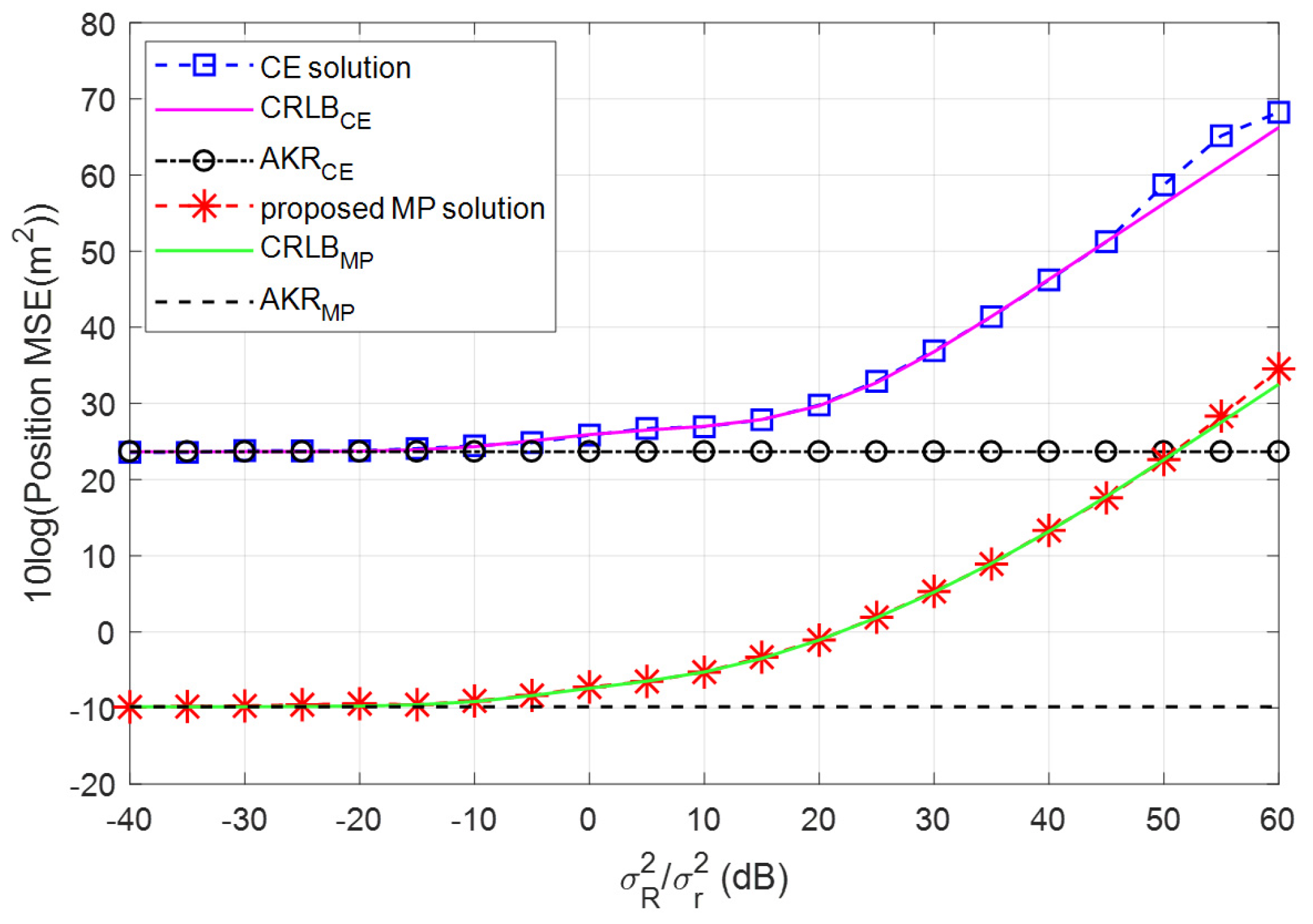
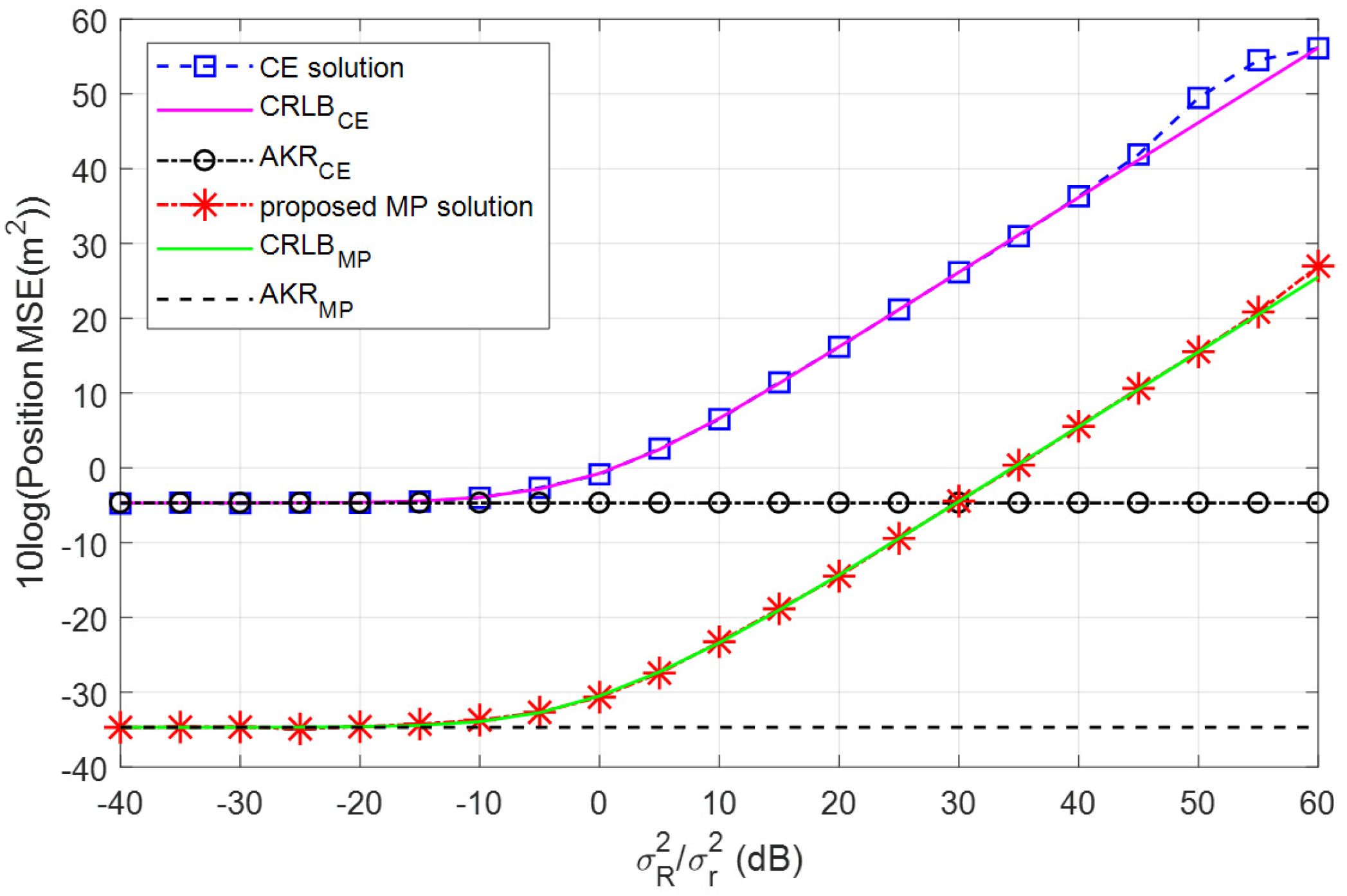
Simulation 1. 

A far underwater acoustic target and a near calibrated source.

Figure 3 shows the performance of the proposed multipath (MP) solution and CE solution [29] as the value of the sensor position error ${\sigma }_s^2/{\sigma }_r^2$ increases, where the distant unknown underwater acoustic source is located at $s=[3000,2300,300]$ and the near calibration source is located at $C_1=[2500,2450,170]$. For the convenience of comparison, the CRLB when the sensor position is accurately known (marked with AKR) is also presented.

The proposed MP closed form and CE solutions follow the CRLB performance well until ${\sigma }_s^2/{\sigma }_r^2=45 \mathrm{dB}$. The thresholding effect occurs earlier in the CE method, which is due to the nonlinear nature of the estimation problem.

Table 1. Efficiency percentage of CE and MP methods (Simulation 1).

${\mathit{\sigma }}_{\mathit{R}}^2/{\mathit{\sigma }}_{\mathit{r}}^2 \left(\mathbf{dB}\right)$		−30	−10	10	30	50
Efficiency percentage (%)	CE	93.2	95.7	89.1	79.3	52.3
	MP	97.3	91.8	94.2	92.9	87.2

displays the percentage efficiency of CE and MP methods across diverse noise levels in the scenario of Simulation 1. Efficiency is defined as the ratio of the estimated positioning error to the CRLB. The results reveal that the efficiency ratio of CE and MP algorithms can exceed 90% under low−noise conditions. However, as the noise level and the CRLB escalate, the algorithm’s efficiency percentage declines, and, the CE’s localization efficiency abruptly drops under moderate noise due to the thresholding effect.

Notably, as the sensor position error increases, the MP method always provides an improvement of about 20 dB in localization performance. This is attributable to the introduction of virtual sensors and source calibration in the MP method, which greatly reduces the CRLB of the multipath method and hence significantly improves localization performance.

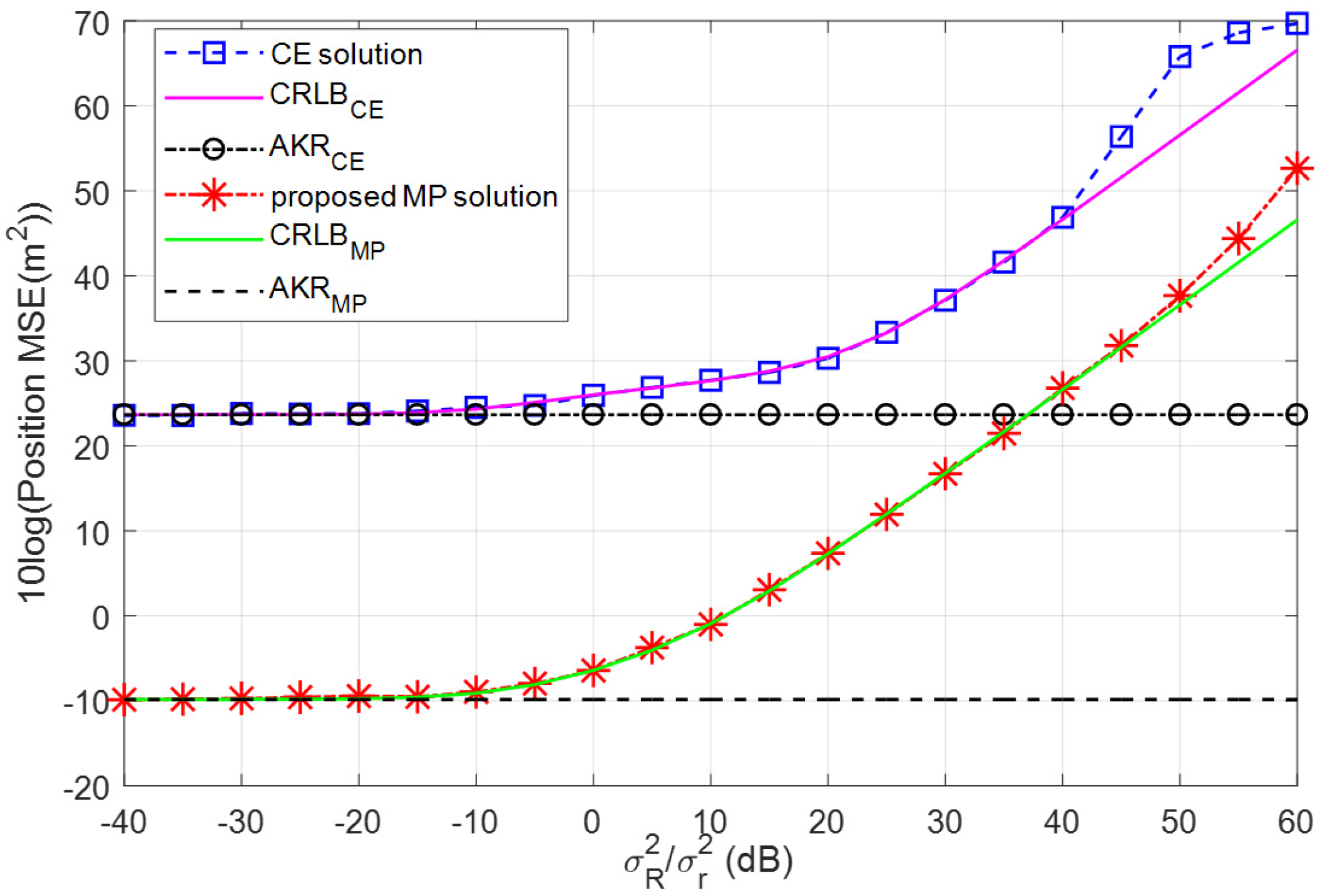
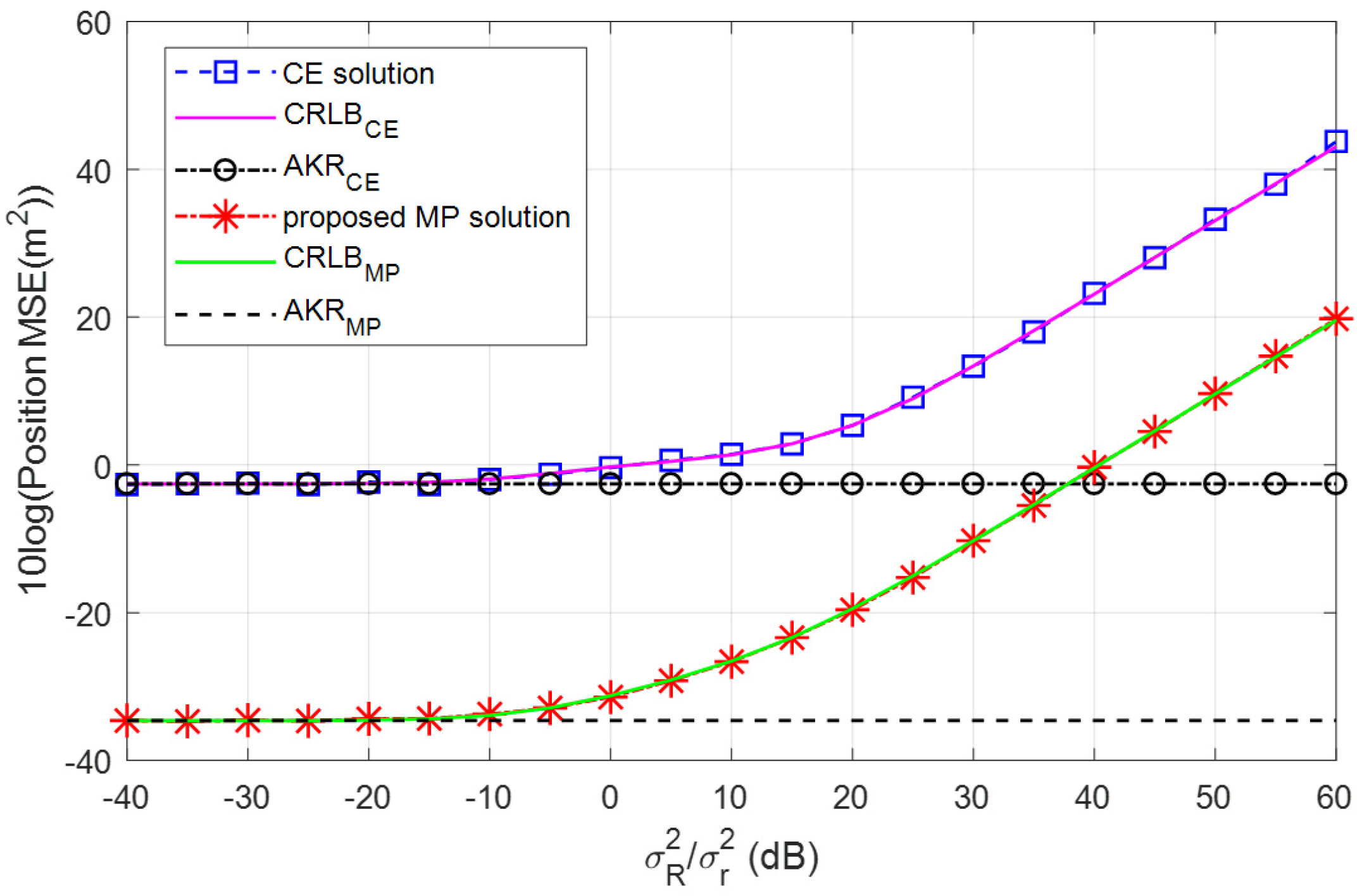
Simulation 2. 

A far underwater acoustic target and a far calibrated source.

The conditions shown in Figure 4 are consistent with those shown in Figure 3 except that the calibration source is located at $C_2=[300,500,200]$, farther away from the underwater acoustic source. The proposed multipath and CE solutions follow the performance well when the value is ${\sigma }_s^2/{\sigma }_r^2\le 45 \mathrm{dB}$. Moreover, the MP solution has better behavior in staying with the CRLB when the sensor position error is large, while the performance of the CE method suddenly deteriorates. This is because the calibration source is far away from the acoustic source, which greatly reduces the overall positioning accuracy, resulting in the thresholding effect that appears earlier compared to Simulation 1.

The results presented in

Table 2. Efficiency percentage of CE and MP methods (Simulation 2).

${\mathit{\sigma }}_{\mathit{R}}^2/{\mathit{\sigma }}_{\mathit{r}}^2 \left(\mathbf{dB}\right)$		−30	−10	10	30	50
Efficiency percentage (%)	CE	94.9	87.9	89.1	63.3	22.3
	MP	92.1	93.5	95.7	86.9	79.6

demonstrate that in this simulation scenario, the MP method achieves a positioning efficiency of over 80% under moderate noise, which outperforms the CE algorithm by a considerable margin. This is due to the CE algorithm’s performance deterioration with increased distance from the calibration source, while the MP method offers distinct advantages. Moreover, the MP method exhibits better adherence to the CRLB and consistently maintains high efficiency, making it superior in the general trend.

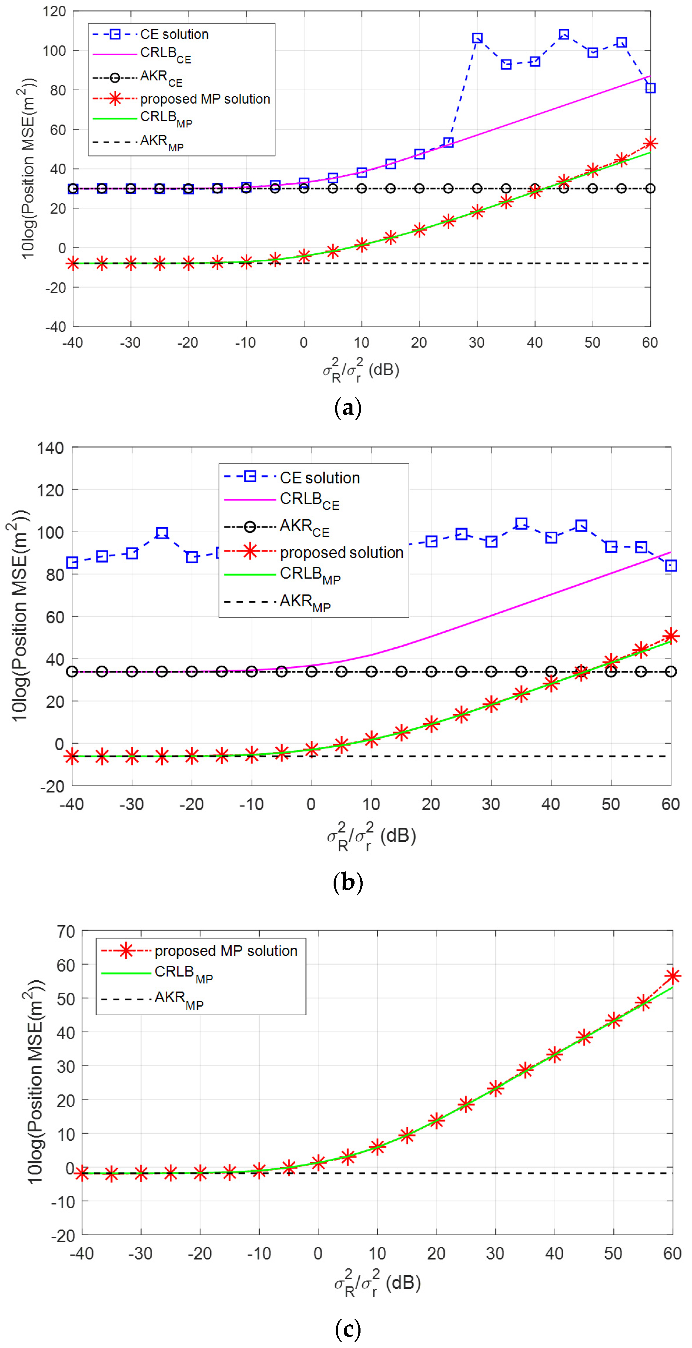
Simulation 3. 

A near underwater acoustic target and a far calibration source.

Simulation 4. 

A near underwater acoustic target and a far calibration source.

Figure 5 and Figure 6 compare the performance of the two algorithms when the target source is located at $s=[550,780,-200]$ closer to the sensor array and the calibration source is located at $C_1$ and $C_2$, respectively. This again verifies that the estimated performance is better when the calibration source is closer to the underwater acoustic source. By comparing these two figures with Figure 3 and Figure 4, it can be seen that the performance of the near source is much better than that of the far source and that the thresholding effect appears later. The thresholding phenomenon here refers to the estimation performance that could suddenly deviate from the optimum accuracy defined by the CRLB when the noise level becomes large or when the source is moving away from the sensors. This is because the classical TDOA localization algorithm estimates the position of the target under the near-field assumption while the target is far away from the sensor network. As a result, the performance of the algorithm will deteriorate to varying degrees.

Table 3. Efficiency percentage comparison table for CE and MP methods (Simulation 3).

${\mathit{\sigma }}_{\mathit{R}}^2/{\mathit{\sigma }}_{\mathit{r}}^2 \left(\mathbf{dB}\right)$		−30	−10	10	30	50
Efficiency percentage (%)	CE	93.4	91.6	96.2	89.7	61.3
	MP	96.8	93.9	95.1	92.6	89.9

and

Table 4. Efficiency percentage of CE and MP methods (Simulation 4).

${\mathit{\sigma }}_{\mathit{R}}^2/{\mathit{\sigma }}_{\mathit{r}}^2 \left(\mathbf{dB}\right)$		−30	−10	10	30	50
Efficiency percentage (%)	CE	93.7	91.2	95.1	89.3	85.8
	MP	92.3	96.2	96.7	93.1	90.9

reveal that both the CE and MP algorithms exhibit high efficiency in the Simulations 3 and 4 scenarios, despite the rapid decline in the efficiency of the CE algorithm due to the threshold effect. The MP method exhibits an efficiency of over 90%, while the CE algorithm achieves an efficiency of more than 80% prior to the onset of the thresholding effect. It is important to note that the proposed algorithm in this paper outperforms other methods in terms of adhering to the CRLB by consistently maintaining a CRLB advantage of approximately 30 dB. These results suggest that the proposed algorithm is a more suitable choice for localization applications in these scenarios.

Simulation 5: 

Minimum number of sensors.

In this scenario, the target source is located at $s=[550,780,-200]$ closer to the sensor array, with the near calibration source located at $C_1=[2500,2450,170]$. We compare the performance of both algorithms using simulations for 5, 4, and 3 sensors.

As illustrated in Figure 7, when the number of sensors is 5, the thresholding effect of the CE method appears when the sensor position error is very small. When the number of sensors is reduced to 4, the CE algorithm becomes inapplicable, as it fails to estimate the location of the sound source.

However, in sharp contrast, the MP method can follow the CRLB well in all three subgraphs, and ideal positioning performance can be achieved by using just 3 sensors due to the introduction of virtual sensors. This breaks the limitation that at least 5 sensors are required for TSWLS-based methods in a 3D space.

Table 5. Efficiency percentage of the CE and MP methods (Simulation 5).

${\mathit{\sigma }}_{\mathit{R}}^2/{\mathit{\sigma }}_{\mathit{r}}^2 \left(\mathbf{dB}\right)$			−30	−10	10	30	50
Efficiency percentage (%)	5 sensors	CE	92.0	93.7	87.5	12	— 1
		MP	97.3	95.1	97.1	93.5	88.5
	4 sensors	CE	—	—	—	—	—
		MP	95	90	87.5	81.3	75.3
	3 sensors	CE	—	—	—	—	—
		MP	89.3	93.2	86.5	80.3	78.2

¹ An em dashe (—) indicate that the algorithm is invalid in this case.

shows that with a reduction in the number of sensors to 4 or 3, the CE algorithm becomes unsuitable for sound source localization, while the MP algorithm maintains an efficiency of over 90% in low noise and above 80% in moderate noise. This is because the CE algorithm relies on intermediate variables and requires at least 5sensors for accurate localization, whereas the MP algorithm utilizes virtual sensors to enhance TDOA measurement information, making it effective even with only 3 sensors and ensuring high localization efficiency.

7. Conclusions

This paper presents an improved UWAL multipath method using the WSL method based on TDOA measurements, which solves the problem of lack of observation data and floating sensor position in UWAL. The multipath method increased the number of sensors by using the multipath nature of the underwater environment. At the same time, a single calibration emission source with a known position is introduced to correct the sensor position and improve positioning accuracy.

In the first stage of the algorithm, multipath signals are introduced to increase the number of virtual elements, and a single calibration transmitting source is used to correct the sensor position error to obtain a more accurate sensor position. In the second stage, the nuisance variables are introduced to obtain the initial estimation of the underwater object. In the final stage, the performance of the estimator is improved by using the nonlinear relationship between the nuisance variables. The CRLB is also derived for the positioning scenario in this paper. Theoretical analysis and simulation confirm that the proposed algorithm can reach the CRLB at a low-noise level.

In addition, the proposed algorithm breaks through the limitation that the traditional TDOA algorithm needs at least four sensors for positioning in a 3D space. The proposed algorithm can locate the target with only three sensors, and the localization accuracy can still reach the CRLB under conditions of small noise.

In underwater localization scenarios, the accuracy of TDOA-based positioning systems can be significantly affected by the uncertainty of sound propagation speed. Since various factors such as temperature, pressure, and salinity affect underwater acoustic propagation speed, developing robust algorithms for real-time estimation of propagation speed based on environmental factors is a potential direction for future research. Machine learning techniques can also be incorporated into these algorithms to study the relationship between environmental factors and propagation speed and improve the accuracy of estimation. Another direction for future research is to investigate the impact of acoustic propagation speed uncertainty on the performance of TDOA-based positioning systems. Quantifying the influence of speed uncertainty on the accuracy of TDOA-based positioning systems can help in developing appropriate mitigation strategies to account for this uncertainty.

In summary, developing algorithms for real-time estimation of acoustic propagation speed and investigating the impact of acoustic propagation speed can contribute to enhancing the accuracy of TDOA-based positioning systems in underwater environments.

References

1. Zhu, M.; Zhao, Y.; Zhang, C.; Ying, P. High Precision Positioning for Searching Airborne Black Boxes Underwater Based on Acoustic Orbital Angular Momentum. In Proceedings of the 2018 IEEE/AIAA 37th Digital Avionics Systems Conference (DASC), London, UK, 23–27 September 2018. [Google Scholar]
2. Sun, S.; Zhang, X.; Zheng, C.; Fu, J.; Zhao, C. Underwater Acoustical Localization of The Black Box Utilizing Single Autonomous Underwater Vehicle Based On The Second-Order time Difference of Arrival. IEEE J. Ocean. Eng. 2020, 45, 1268–1279. [Google Scholar] [CrossRef]
3. Wang, Y.; Huang, X.; Cao, R. Novel Approach for ISAR Cross-Range Scaling Based on the Multi-delay Discrete Polynomial-Phase Transform Combined with Keystone Transform. IEEE Trans. Geosci. Remote Sens. 2020, 58, 1221–1231. [Google Scholar] [CrossRef]
4. Khaled, H.A.; Shitharth, S.; Hariprasath, M.; Adil, O.K.; Alaa, O.K. Connotation of fuzzy logic system in Underwater communication systems for navy applications with data indulgence route. Sustain. Comput. Inform. Syst. 2023, 38, 100862. [Google Scholar]
5. Kshirsagar, P.R.; Manoharan, H.; Shitharth, S.; Alshareef, A.M.; Singh, D.; Lee, H.-N. Probabilistic Framework Allocation on Underwater Vehicular Systems Using Hydrophone Sensor Networks. Water 2022, 14, 1292. [Google Scholar] [CrossRef]
6. Manoharan, H.; Shitharth, S.; Sangeetha, K.; Kumar, B.P. Mustapha Hedabou, Detection of superfluous in channels using data fusion with wireless sensors and fuzzy interface algorithm. Measurement. Sensors 2022, 23, 100405. [Google Scholar]
7. Tan, H.P.; Diamant, R.; Seah, W.; Waldmeyer, M. A survey of techniques and challenges in underwater localization. Ocean Eng. 2011, 38, 1663–1676. [Google Scholar] [CrossRef]
8. Zia, M.I. State-of-the-Art Underwater Acoustic Communication Modems: Classifications, Analyses and Design Challenges. Wirel. Pers. Commun. 2021, 116, 1325–1360. [Google Scholar] [CrossRef]
9. Sendra, S.; Lloret, J.; Jimenez, J.M.; Parra, L. Underwater Acoustic Modems. IEEE Sens. J. 2016, 16, 4063–4071. [Google Scholar] [CrossRef]
10. Agheli, P.; Beyranvand, H.; Emadi, M.J. UAV-Assisted Underwater Sensor Networks using RF and Optical Wireless Links. J. Light. Technol. 2021, 39, 070–7082. [Google Scholar] [CrossRef]
11. Zhu, Z.; Hu, S. Model and Algorithm Improvement on Single Beacon Underwater Tracking. IEEE J. Ocean. Eng. 2017, 43, 1143–1160. [Google Scholar] [CrossRef]
12. Bayat, M.; Crasta, N.; Aguiar, A.P.; Pascoal, A.M. Range-Based Underwater Vehicle Localization in the Presence of Unknown Ocean Currents: Theory and Experiments. IEEE Trans. Control Syst. Technol. 2016, 24, 122–139. [Google Scholar] [CrossRef]
13. Heidemann, J.; Stojanovic, M.; Zorzi, M. Underwater sensor networks: Applications, advances and challenges. Philos. Trans. R. Soc. A Math. Phys. Eng. Sci. 2012, 370, 158. [Google Scholar] [CrossRef] [PubMed]
14. Sun, S.; Liu, T.; Wang, Y.; Zhang, G.; Liu, K. High-Rate Underwater Acoustic Localization Based on the Decision Tree. IEEE Trans. Geosci. Remote Sens. 2022, 60, 4204912. [Google Scholar] [CrossRef]
15. Diez-Gonzalez, J.; Avarez, R.; Verde, P.; Ferrero-Guillen, R.; Perez, H. Analysis of reliable deployment of TDOA local positioning architectures. Neurocomputing 2022, 484, 149–160. [Google Scholar] [CrossRef]
16. Yu, H.; Huang, G.; Gao, J.; Liu, B. An Efficient Constrained Weighted Least Squares Algorithm for Moving Source Location Using TDOA and FDOA Measurements. IEEE Trans. Wirel. Commun. 2012, 11, 44–47. [Google Scholar] [CrossRef]
17. Foy, W.H. Position-Location Solutions by Taylor-Series Estimation. IEEE Trans. Aerosp. Electron. Syst. 2007, 12, 187–194. [Google Scholar] [CrossRef]
18. Mandic, F.; Miskovic, N.; Loncar, I. Underwater Acoustic Source Seeking Using Time-Difference-of-Arrival Measurements. IEEE J. Ocean. Eng. 2020, 45, 759–771. [Google Scholar] [CrossRef]
19. Liang, Q.; Zhan, B.; Zhao, C. TDoA for Passive Localization: Underwater versus Terrestrial Environment. IEEE Trans. Parallel Distrib. Syst. 2013, 24, 2100–2108. [Google Scholar] [CrossRef]
20. Carvalho, W.; Antonio, J. An Emitter Localization Method Based on Multiple Differential Doppler Measurements. IEEE Latin Am. Trans. 2022, 20, 537–544. [Google Scholar]
21. Pei, Y.; Li, X.; Yang, L.; Guo, F. A Closed-Form Solution for Source Localization Using FDOA Measurements Only. IEEE Commun. Lett. 2023, 27, 115–119. [Google Scholar] [CrossRef]
22. Qi, H.; Wu, X.; Jia, L. Semidefinite Programming for Unified TDOA-based Localization Under Unknown Propagation Speed. IEEE Commun. Lett. 2020, 24, 1971–1975. [Google Scholar] [CrossRef]
23. Dai, Z.; Wang, G.; Chen, H. Sensor Selection for TDOA-Based Source Localization Using Angle and Range Information. IEEE Trans. Aerosp. Electron. Syst. 2021, 57, 2597–2604. [Google Scholar] [CrossRef]
24. Chan, Y.; Ho, K. A simple and efficient estimator for hyperbolic location. IEEE Trans. Signal Process. 2002, 42, 1905–1915. [Google Scholar] [CrossRef]
25. Rui, L.; Ho, K. Efficient closed-form estimators for multistatic sonar localization. IEEE Trans. Aerosp. Electron. Syst. 2015, 51, 600–614. [Google Scholar] [CrossRef]
26. Sandys-Wunsch, M.; Hazen, M.G. Multistatic localization error due to receiver positioning errors. IEEE J. Ocean. Eng. 2002, 27, 328–334. [Google Scholar] [CrossRef]
27. Ho, K.C.; Lu, X.; Kovavisaruch, L. Source Localization Using TDOA and FDOA Measurements in the Presence of Receiver Location Errors: Analysis and Solution. IEEE Trans. Signal Process. 2007, 55, 684–696. [Google Scholar] [CrossRef]
28. Gong, Z.; Li, C.; Jiang, F. Analysis of the Underwater Multi-Path Reflections on Doppler Shift Estimation. IEEE Wirel. Commun. Lett. 2020, 9, 1758–1762. [Google Scholar] [CrossRef]
29. Ho, K.C.; Le, Y. On the Use of a Calibration Emitter for Source Localization in the Presence of Sensor Position Uncertainty. IEEE Trans. Signal Process. 2008, 56, 5758–5772. [Google Scholar] [CrossRef]
30. Huang, B.; Xie, L.; Yang, Z. TDOA-Based Source Localization with Distance-Dependent Noises. IEEE Trans. Wirel. Commun. 2015, 14, 468–480. [Google Scholar] [CrossRef]
31. Emokpae, L.E.; Dibenedetto, S.; Potteiger, B.; Younis, M. UREAL: Underwater Reflection-Enabled Acoustic-Based Localization. IEEE Sens. J. 2014, 14, 3915–3925. [Google Scholar] [CrossRef]
32. Prasad, K.V. Fundamentals of statistical signal processing: Estimation theory. Control Eng. Pract. 1994, 2, 728. [Google Scholar] [CrossRef]
33. Sun, Y.; Ho, K.C.; Wan, Q. Solution and Analysis of TDOA Localization of a Near or Distant Source in Closed Form. IEEE Trans. Signal Process. 2019, 67, 320–335. [Google Scholar] [CrossRef]
Figure 1. Underwater multipath signal location scenario.
Jmse 11 00861 g001
Figure 2. Implementation flow of unknown source localization.
Jmse 11 00861 g002
Figure 3. Performance of a far acoustic target and a near calibration source.
Jmse 11 00861 g003
Figure 4. Performance of a far acoustic target and a far calibration source.
Jmse 11 00861 g004
Figure 5. Performance of a near acoustic target and a far calibration source.
Jmse 11 00861 g005
Figure 6. Performance of a near acoustic target and a near calibration source.
Jmse 11 00861 g006
Figure 7. Performance with different numbers of sensors: (a) 5 sensors, (b) 4 sensors, (c) 3 sensors.
Jmse 11 00861 g007