A New Coastal Crawler Prototype to Expand the Ecological Monitoring Radius of OBSEA Cabled Observatory

Abstract

The use of marine cabled video observatories with multiparametric environmental data collection capability is becoming relevant for ecological monitoring strategies. Their ecosystem surveying can be enforced in real time, remotely, and continuously, over consecutive days, seasons, and even years. Unfortunately, as most observatories perform such monitoring with fixed cameras, the ecological value of their data is limited to a narrow field of view, possibly not representative of the local habitat heterogeneity. Docked mobile robotic platforms could be used to extend data collection to larger, and hence more ecologically representative areas. Among the various state-of-the-art underwater robotic platforms available, benthic crawlers are excellent candidates to perform ecological monitoring tasks in combination with cabled observatories. Although they are normally used in the deep sea, their high positioning stability, low acoustic signature, and low energetic consumption, especially during stationary phases, make them suitable for coastal operations. In this paper, we present the integration of a benthic crawler into a coastal cabled observatory (OBSEA) to extend its monitoring radius and collect more ecologically representative data. The extension of the monitoring radius was obtained by remotely operating the crawler to enforce back-and-forth drives along specific transects while recording videos with the onboard cameras. The ecological relevance of the monitoring-radius extension was demonstrated by performing a visual census of the species observed with the crawler’s cameras in comparison to the observatory’s fixed cameras, revealing non-negligible differences. Additionally, the videos recorded from the crawler’s cameras during the transects were used to demonstrate an automated photo-mosaic of the seabed for the first time on this class of vehicles. In the present work, the crawler travelled in an area of 40 m away from the OBSEA, producing an extension of the monitoring field of view (FOV), and covering an area approximately 230 times larger than OBSEA’s camera. The analysis of the videos obtained from the crawler’s and the observatory’s cameras revealed differences in the species observed. Future implementation scenarios are also discussed in relation to mission autonomy to perform imaging across spatial heterogeneity gradients around the OBSEA.

1. Introduction

With more than two-thirds of our planet covered by water at depths limiting or beyond direct human reach, our knowledge of the biodiversity and functioning of marine ecosystems is limited [1]. To fill this knowledge gap, the use of autonomous technologies delivering long-lasting and complexly interrelated biological and environmental data is required to describe the diffusion of impacts across the hydrosphere and the geosphere [2,3,4,5]. More traditional and advanced platform designs such as Remotely Operated Vehicles (ROVs; [6]), Autonomous Underwater Vehicles (AUVs; [7]), Autonomous Surface Vehicles (ASVs; [8]), or drifters [9] are being used not only for ecosystem explorations but also for innovative monitoring approaches with repeated measurements across different geographic scales [10], allowing advanced management policies [11,12]. Their powerful multiparametric biological, oceanographic, and geochemical high-spatial-resolution data collection capabilities are combined with spatially expanded navigation over both the seabed [13] and the water column [14]. In this scenario, underwater imaging (e.g., high definition-HD, low-light, and acoustic-multibeam cameras) is increasingly used to quantify the presence, abundance, and behaviour of marine fauna. Imaging sampling approaches serve the needs of biodiversity characterisation as a central factor for management and conservation policies [15,16,17,18,19,20,21].

However, most platforms operate as vessel-assisted units, so their missions fail to capture the changing trends in marine communities at tidal, day-night, and seasonal temporal scales. This is because vessel operation constraints (e.g., work shifts) and high costs impose limitations on the duration of their surveys, favouring spatial coverage and not the repetition of sampling at a specific point [6,22]. However, present data indicate community turnover over 24-h and seasonal scales that are produced by massive population displacements within our sampling windows, due to the variable activity rates in response to reproduction and growth [23,24,25].

Vessel-independent monitoring technologies such as cabled observatories allow for prolonged and autonomous data collection that can be implemented at virtually any depth of the continental margin [26,27,28]. Their deployment implies very high initial costs that can be progressively depreciated over years of continuous data collection [29]. Although their fixed imaging has been extensively used to assess the animals’ abundance, behaviour, biodiversity, and even community successions in many marine areas (e.g., [25,30,31,32,33]), they lack an extensive Field of View (FOV), therefore, the acquired data are not representative of the ecological heterogeneity that surrounds the observatories [27].

This drawback in cabled observatories monitoring capability can be overcome by developing docked mobile platforms [5]. These could be permanently installed to expand their spatial range and resolution, improving the ecological representativeness of their seafloor monitoring [33]. Depending on the specific needs, different platforms could be eligible for that task. Docked propeller-driven pelagic robots, such as ROVs, AUVs, and Autonomous Underwater Helicopters (AUHs) are preferred when medium-long range mobility through rough seabed morphologies must be met [27,34]. However, ROVs will result in a shorter range, due to the limitation of the cable, but provide a higher degree of control over the operations [35,36,37]. In contrast, AUVs would be able to venture further away from the fixed platform, allow more advanced operations, and reduce the need for human operators [38,39,40]. On the other hand, when the priorities include the stability of the mobile platform, the silence of operations, and power consumption, negatively buoyant benthic vehicles (e.g., crawlers [41,42], rovers [43], and bio-inspired Underwater Legged Robots [44]) are preferable.

Regardless of the choice of mobile platform, they can be connected to the cabled video-observatories as an Internet Operated Vehicle (IOV) either for real-time control [45], or autonomously preloaded missions [46]. In particular, thanks to their stability and passive current rejection capabilities, tethered crawlers can act as multi-parametric observatories themselves and can be used to generate geo-referenced, long-term (i.e., multiannual), high-frequency biological (i.e., time-lapse images or video-based photo-mosaics), and multiparametric environmental datasets when standing-still or moving slowly (e.g., stepping-stone mode) [47,48]. In the near future, crawlers will even be able to operate without tethering (i.e., based on autonomous navigation capabilities and communication with other platforms) [21].

Benthic crawlers are generally used in the deep sea. For example, in Barkley Canyon (Canada), Wally has been deployed at a gas hydrate deep-sea site since September 2010 [41,49]. Rossia (an improved version of Wally), was tested in November 2019 to also work in the deep sea [50]. Norppa is another example of a deep-sea crawler designed by Jacobs University (Bremen) that sailed in shallow water while navigating from a ship for a short run [51]. All the aforementioned platforms were designed to work in the deep sea or, in case of shallow water, navigate from a ship, and not independently, for a short run. In this paper, for the first time, we present the integration of a benthic crawler into a coastal cabled observatory (in our case, an OBSEA underwater observatory operating in the north-western Mediterranean for more than a decade [52,53]). We describe the technological design, specifications, and assemblage of its components, as well as their testing in land, pool, and real-world scenarios. We also detail the web-control functionalities to remotely control in real time or program automated back-and-forth drives along specific transects around the observatory. Finally, the capacity of the crawler for mobile ecological monitoring is tested in relation to the description of the local fish community versus the results of concomitant video monitoring by the fixed OBSEA camera, and the results are presented. These results clearly show that, by adding the coastal underwater crawler to the OBSEA observatory, the field of view was drastically expanded, and thus, some different types of species were detected that had not been detected by the OBSEA’s camera. This monitoring is also complemented by examples of automated photo-mosaicking, with a description of the underlying camera calibration and image transformation processes.

The work presented in this paper contributes as a proof of concept and a feasibility development for the JERICO-RI [54] Pilot Supersite (PSS) at the North-West Mediterranean; NW-MED-PSS. PSSs will demonstrate the added values of integrated, state-of-the-art multidisciplinary and multiplatform observation capabilities, develop innovative hierarchical monitoring concepts for coastal seas, and create coastal collaboration platforms for other European environmental Research Infrastructures (RIs), maritime industries, and regional environmental management of coastal ecosystems.

2. Materials and Methods

This section is organised into five subsections, each one treating a different aspect of the proposed crawler’s development: Section 2.1: a description of the OBSEA testing site as an operational context; Section 2.2: a description of the crawler components and their assemblage; Section 2.3: the web architecture for crawler control and the management of acquired video-data; Section 2.4 the image acquisition for automated photo-mosaics; and finally, Section 2.5: the validation of crawler ecological monitoring efficiency.

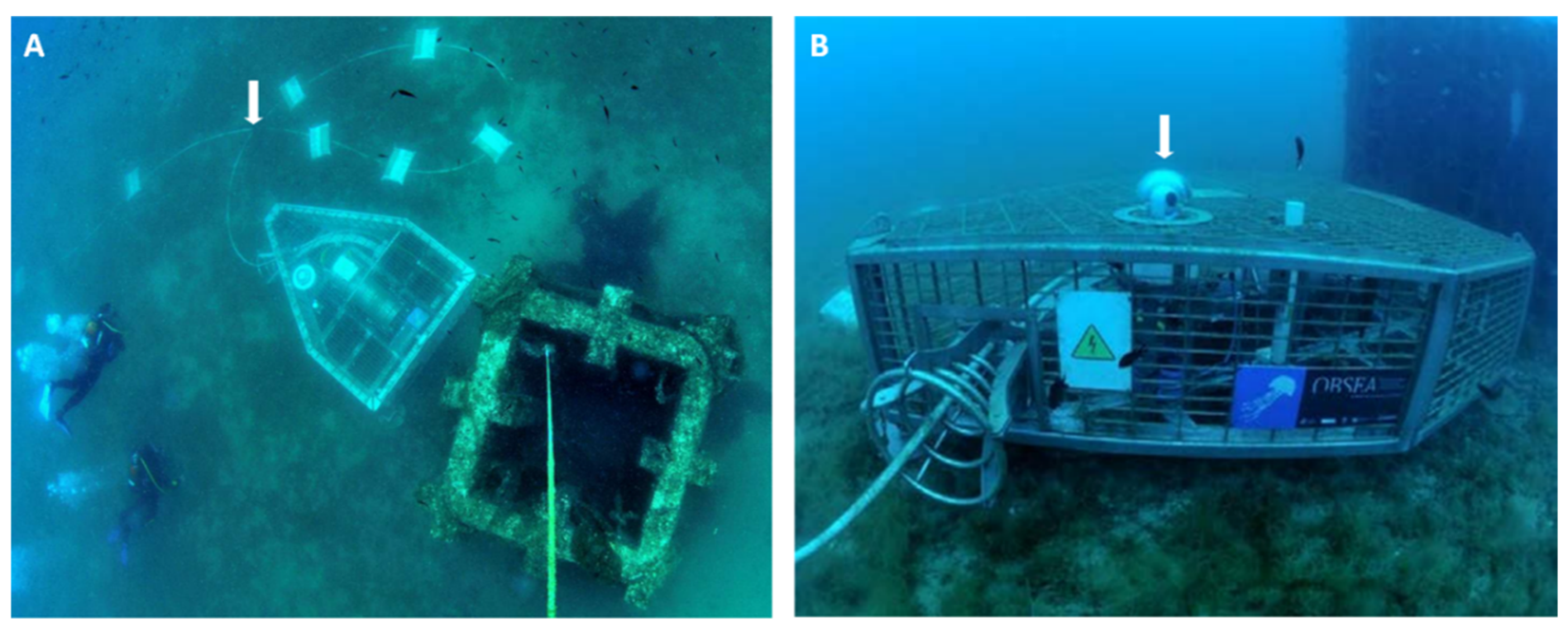
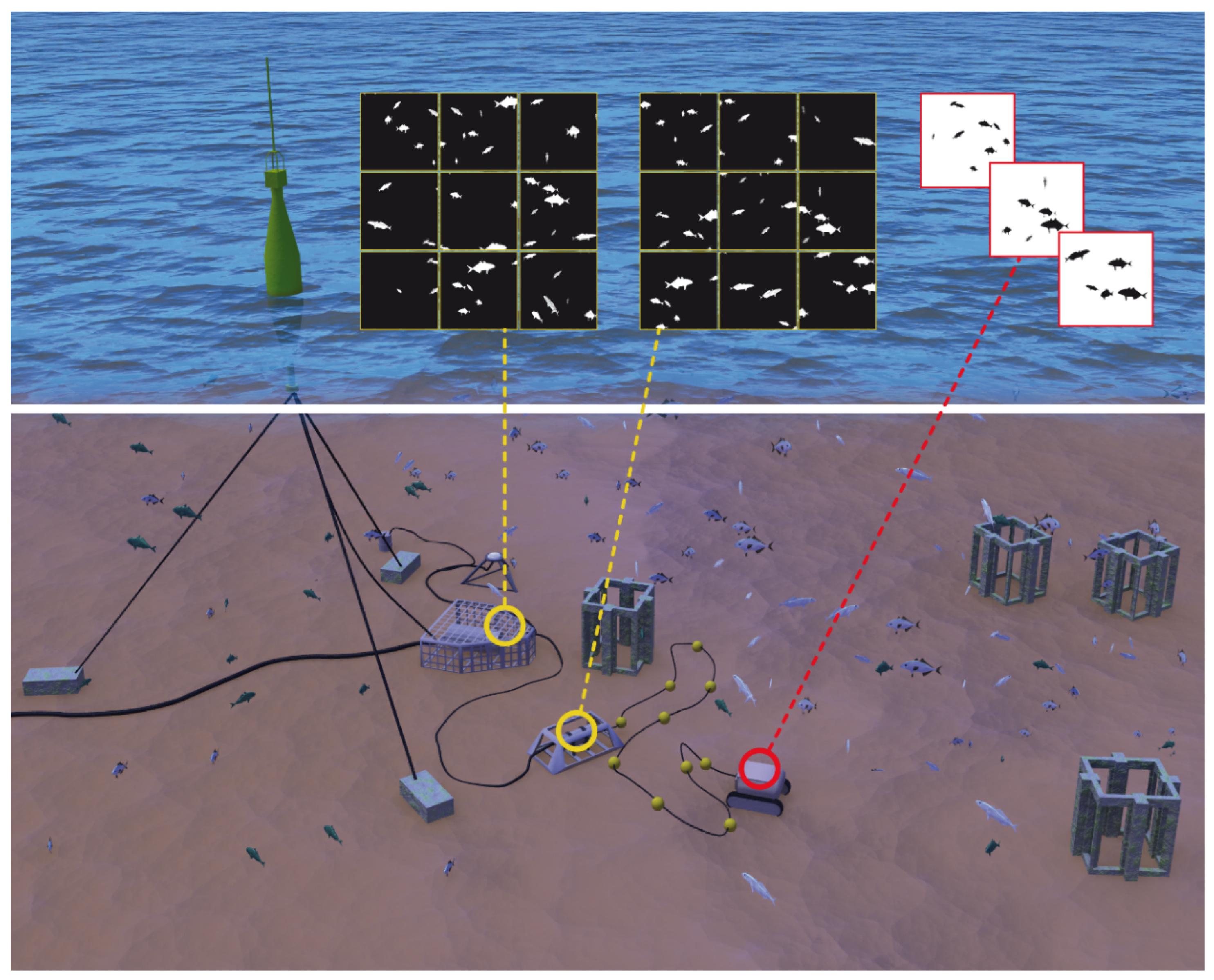
2.1. The OBSEA Test-Site as Operational Context for the Crawler Development

The OBSEA cabled observatory (www.obsea.es, accessed on 10 January 2022), a part of the European Multidisciplinary Seafloor and water-column Observatories (EMSO), is located 4 km from the Vilanova i la Geltrú (Barcelona, Spain) coast, at a depth of 20 m (Figure 1) [52,53]. The OBSEA observatory bears its own HD rotary camera (i.e., a DCS-7010L; resolution of 1280 × 720 pixels), which has been used for day-night image and footage acquisition since 2009 [52]. The platform also bears a set of oceanographic and geochemical sensors such as CTD for salinity and temperature, a fluorometer for chlorophyll-a and turbidity, and an Acoustic Doppler Current Profiler (ADCP) for current speeds and direction metrics [53]. For the first time, crawler monitoring technology will bear an Ultra-Short Base-Line (USBL) acoustic emitter-receiver to allow wireless communications and geolocalisation capabilities with the crawler modem (see the next section), as an intermediate state toward its remote controlling with no tether. The USBL modem is connected to the OBSEA network similarly to other sensors, allowing a remote operator to interrogate and geo-localise the acoustic modem installed on the crawler. In addition, a tripod camera with an umbilical of 800 m branches off the observatory junction box, while a meteorological buoy at the surface provides weather data [55].

The OBSEA operates as the heart of a growing ecological monitoring network (Figure 2), providing power to the other docked platforms connected to the main node [5] and allowing the power and data transfer to and from the crawler (see the next sections). This aspect is of relevance for the replication of data collection over the heterogeneity of the local coastal habitat [27].

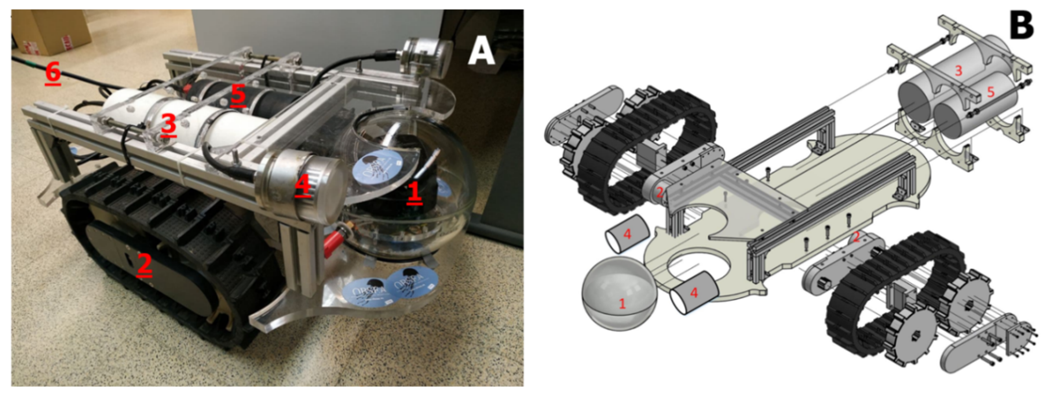
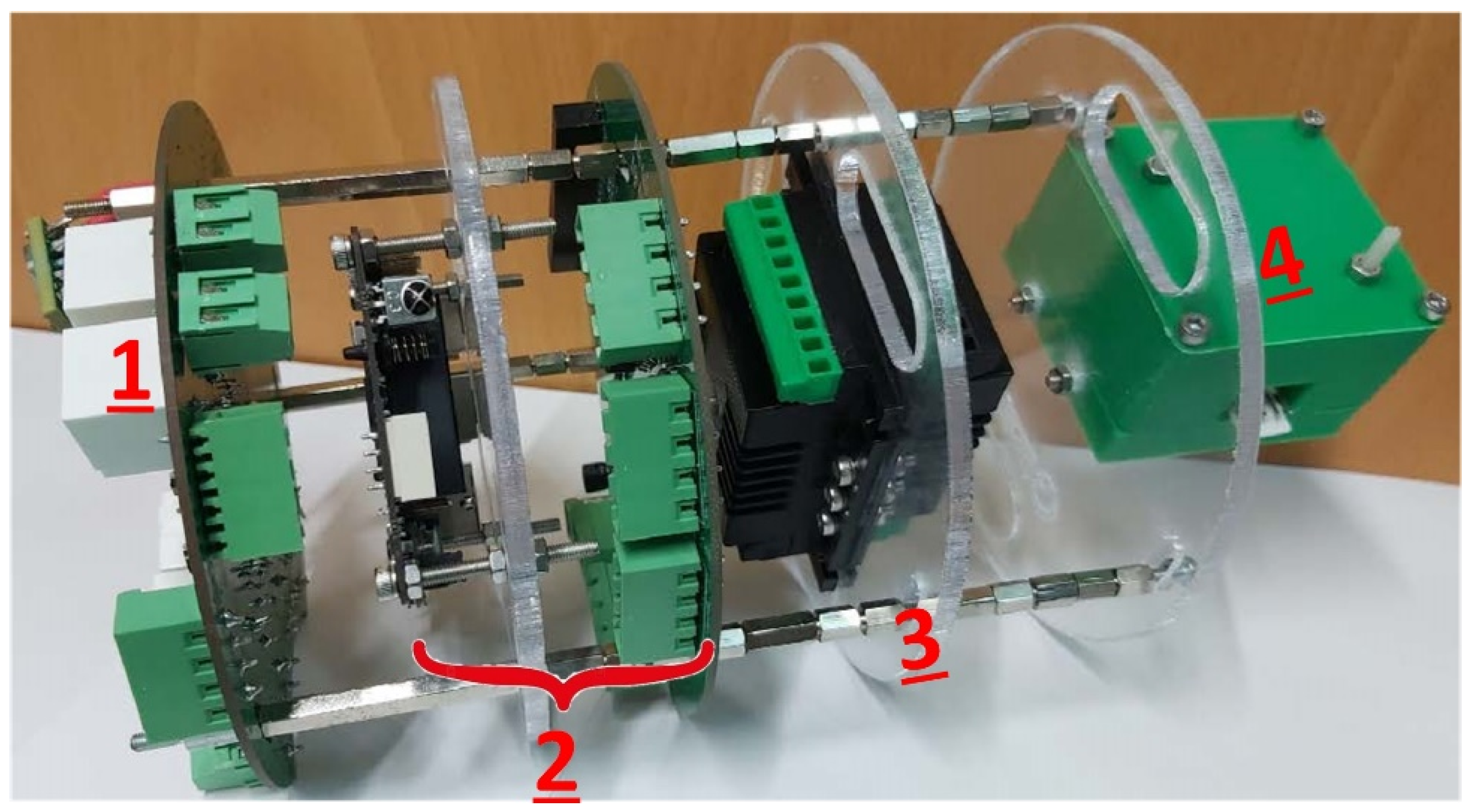
2.2. The Crawler Components and Assemblage

We implemented a new crawler prototype (i.e., width 55 cm, length 100 cm, and height 40 cm, with a total weight in air and in the water of 56 kg and 12.1 kg, respectively) as a modified and lower-cost version of the “Wally” platform; The “Wally” crawler has been operating at the Ocean Networks Canada (ONC; www.oceannetworks.ca, accessed on 18 April 2023) since 2010 [41]. Figure 3 shows the crawler developed for shallow water operations and its various components. The choice of the vehicle and its dimensioning were driven by several factors. Unlike propeller-driven vehicles, which must continuously compensate for current disturbances, benthic crawlers can passively maintain a fixed position, reducing power consumption and acoustic noise during long stationary phases. This is particularly appealing in ecological monitoring operations in which the disturbance introduced by the tool may bias the observation. The dimensions of the crawler resemble those of a typical observation class Remotely Operated Vehicle (ROV; [56]) and allow convenient mobility around the OBSEA, and simple deployment/recovery from a vessel of opportunity.

The crawler is endowed with a new HD camera (SNC-241 RSIA; resolution of 1920 × 1080; 2 megapixels) (see Figure 3, Label 1). This camera can operate at a 180° tilt and 360° pan to allow for a hemispherical panoramic FOV around the platform itself. The camera is installed into a glass sphere, rated up to 3000 m depth, in the front part of the crawler. Two white LED lights (ExtraStar) are placed aside, on top of the camera.

The tracks, which are mounted on a broader chassis (see Figure 3, Label 2), are independent parts that allow the mobilisation of the inner part of the vehicle. A Faulhaber DC motor with a reduction gear of 989:1 was used as a propulsion system for each track. The motor housing is oil-filled and can operate at up to a 100 m depth. The crawler is equipped with two watertight cylinders, one hosting the main control unit and electronics (see Figure 3, Label 3), and the other hosting the power supply unit and the Ethernet switch (see Figure 3, Label 5) connected to the cabled observatory. The main unit (see Figure 3, Label 3) is also in charge of running the crawler, providing control for the motors, measurements of the internal sensors, and control of external instruments such as the HD camera, lights (see Figure 3, Label 4), and S2C—Evologic R 18/34 acoustic modem. The current housing is rated for operations at depths up to 100 m. Furthermore, the main cable (see Figure 3, Label 6) is a 50 m long underwater umbilical cable, designed to be used in deep-water, subsea applications, for transmission data and preparing electrical power. The cable was endowed with foam floaters (190 mm in diameter and buoyancy of 1800 g) to reduce drag, prevent entanglement and abrasion on the seabed, and so as to not impair the platform navigation functionalities.

In order to achieve both driving autonomy and the onboard processing of images and videos to derive high-value ecological monitoring data (see below), we developed a main controller. This was based on a Single-Board Computer (SBC) using an ODROID C4 plate [57]. Although the efficiency of this implementation is described here only in relation to navigation autonomy (see the next section), this board has also been selected because of its potential to autonomously process data onboard. That processing autonomy capability is required for automated fish species identification, classification, and tracking.

Technical specifications for the crawler components, in terms of brand, voltage, and power consumption, are detailed in

Table 1. The crawler component specifications in terms of brand, power consumption, and detailed costs (plus the total).

Element	Brand	Nominal Voltage (V)	Power Consumption (W)	Costs (EUR)
Controller	ODROID C4	12	5	80
Camera	SNC-241RSIA	48	23	750
Lights	ExtraStar (LED)	12	8	2 × 200
Motor Controller	Faulhaber SC5008S	12	2	2 × 275
Motor	Faulhaber 3564K 048B	48	126	2 × 785
Compass	CMPS01	5	1	50
Electrical Boards	Easy EDA (PCB)	48,12	2	200
Acoustic Modem	S2C—Evologic	24	5.5	8000
Cable and Connectors	Falmat (FM022208-01)	Up to 600	---	7000
Structure and Mechanical Parts	---	---	---	9400
Total				EUR 28,000

where we also detail the overall costs of our implementation to provide a range of the economic costs required to create other similar platforms. The “Structure and Mechanical Parts” category in this table includes the chassis, switch, and control cylinder housings, aluminium frame, tracks, camera sphere glass housing, support, and motor housings. “Additional Costs” include specific oil used for filling the motor housing, resin, 3D printed components, the Plexiglas chassis, etc.

The control cylinder (Figure 4) is divided into four main components: a power supply board (see Figure 4, Label 1) to provide the energy for the motor drivers, motors, lights, and compass, and the main controller board. In the main controller board (see Figure 4, Label 2), the ODROID C4 and the backplate board, which provide connections with all the other elements, are included. Moreover, there are two motor drivers (see Figure 4, Label 3) to supply the left and right tracks. Finally, a compass (see Figure 4, Label 4) is used for navigation.

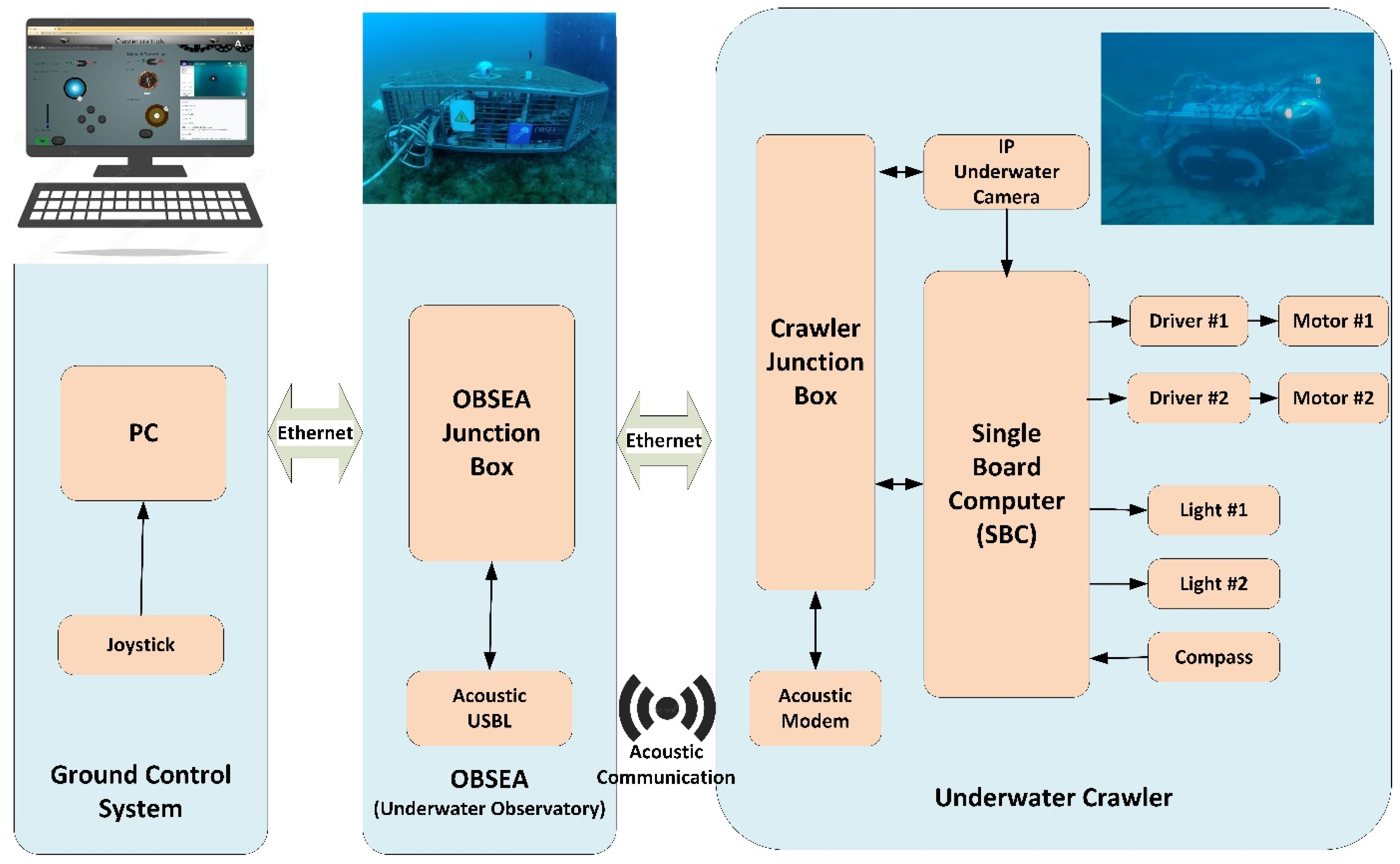
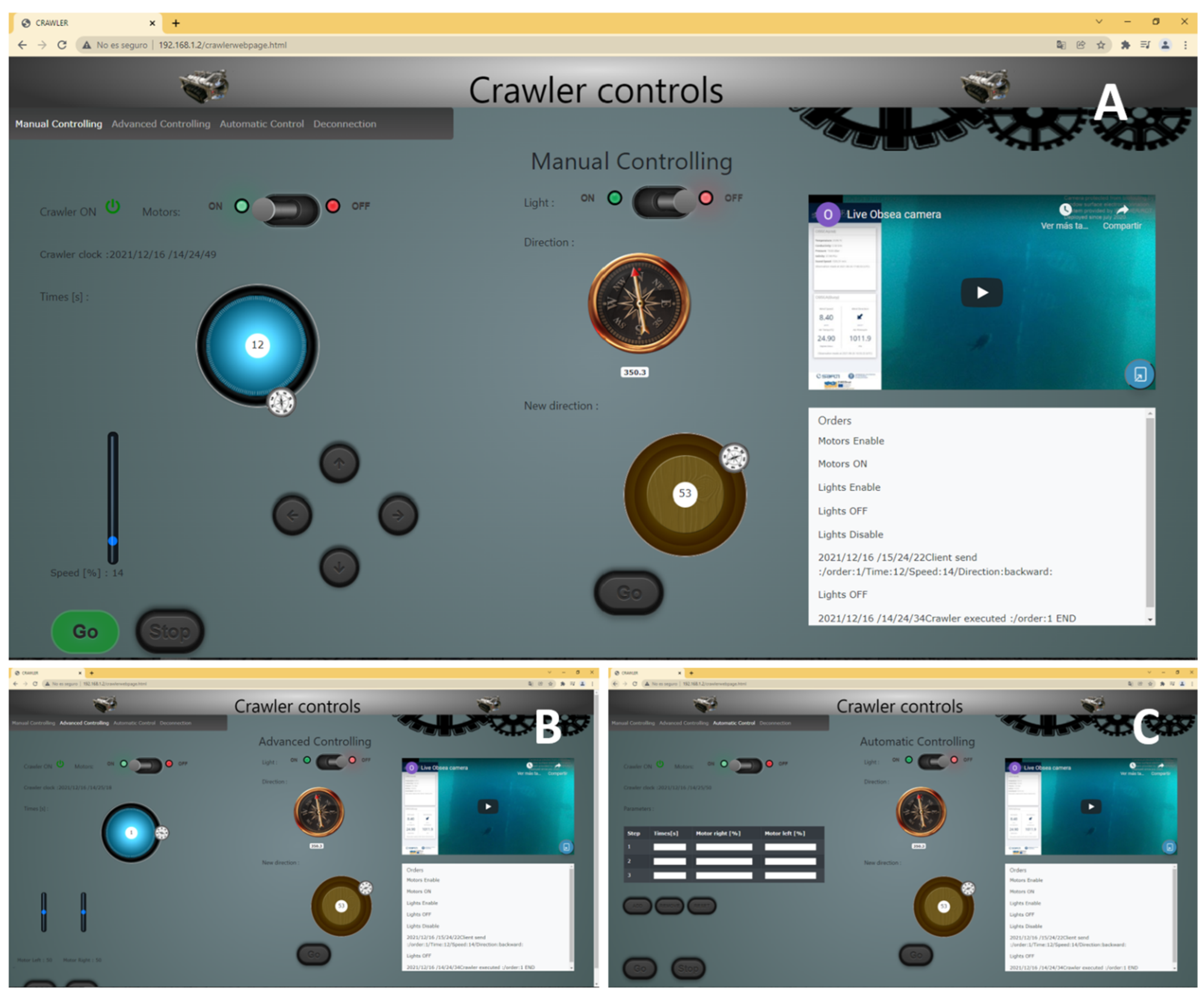
2.3. The Web Architecture for the Crawler Control and the Management of Acquired Video-Data

A web scheme, describing the architecture for the remote control of the crawler navigation and video camera plus light functionalities, is presented in Figure 5. The main idea is to provide one accredited user at a time with an online connection to the crawler via the Internet web portal of the OBSEA (see next paragraph). With that access, the user can remotely control the crawler’s motors, HD camera, lights, and acoustic modem components. The user could also modify navigation pathways by transecting speed and direction in real time.

At the same time, remote control could be exerted on imaging acquisition in terms of light ON and OFF settings under different environmental conditions (i.e., cloudiness or night-time). In addition, the user could set the specifications for time-lapse footage or image acquisition. Other oceanographic and geochemical sensors that could be installed in the future (e.g., CTD for temperature and salinity, or PAR for light intensity within the range of 400–700 nm) would acquire data at the frequency specified by the fabricant.

A web page application (https://crawler.obsea.es, accessed on 18 April 2023) was developed to allow manual, advanced, and automatic control of navigation missions (Figure 6). In all these three navigation modes, there are four common functionalities: a compass pointer for direction, buttons to run and stop the crawler and turn the lights and motors on and off, a window to show the real-time streaming video, and finally, a blank window to show the commands that are being executed. On the manual tab, an accredited user can connect to the web page and drive the crawler by using manual control. The manual mode control works by sending a pair of PWM signals to the motors to move the crawler in the desired direction and during a specified time. On the advanced tab, each motor can move separately and in the desired direction at different speeds. In this mode, each motor can be moved separately, receiving a different amount of PWM signal, and during a desired time. The last mission tab is the automatic control mode, which allows for performing a predefined sequence of orders continuously, enabling the repetition of pre-defined routines by sending a sequence of predefined PWM signals to the motors.

The webpage application for piloting the crawler can only be accessed with institutionally provided credentials (by SARTI-UPC). Data encryption aspects will be taken into account in subsequent developments in response to increased use of the platform.

The camera transmits the video in real time, through a TCP port, and reaches a live channel created on YouTube (https://youtu.be/4q7eyET6rvY, accessed on 18 April 2023). At the same time, the camera itself carries a basic app created by the manufacturer that has been modified and updated in terms of configuration and improved image capture and extraction (see below). All images and videos are archived on the OBSEA online repository, ordered according to a timestamp, and downloaded upon a query. Briefly, the OBSEA camera is catechised at a time interval of 30 min by a specific software application. Acquired images are labelled with a “year:month:day:h:min:s” timestamp (in UTC) and stored on an image bank that allows their later retrieval upon a temporal query. Similarly, crawler images acquired by the ODROID C4 controller, are labelled upon the timestamp of that controller, identically to the system used for the OBSEA camera. All images (or videos) by both platforms’ cameras can be temporally collated in the same video bank.

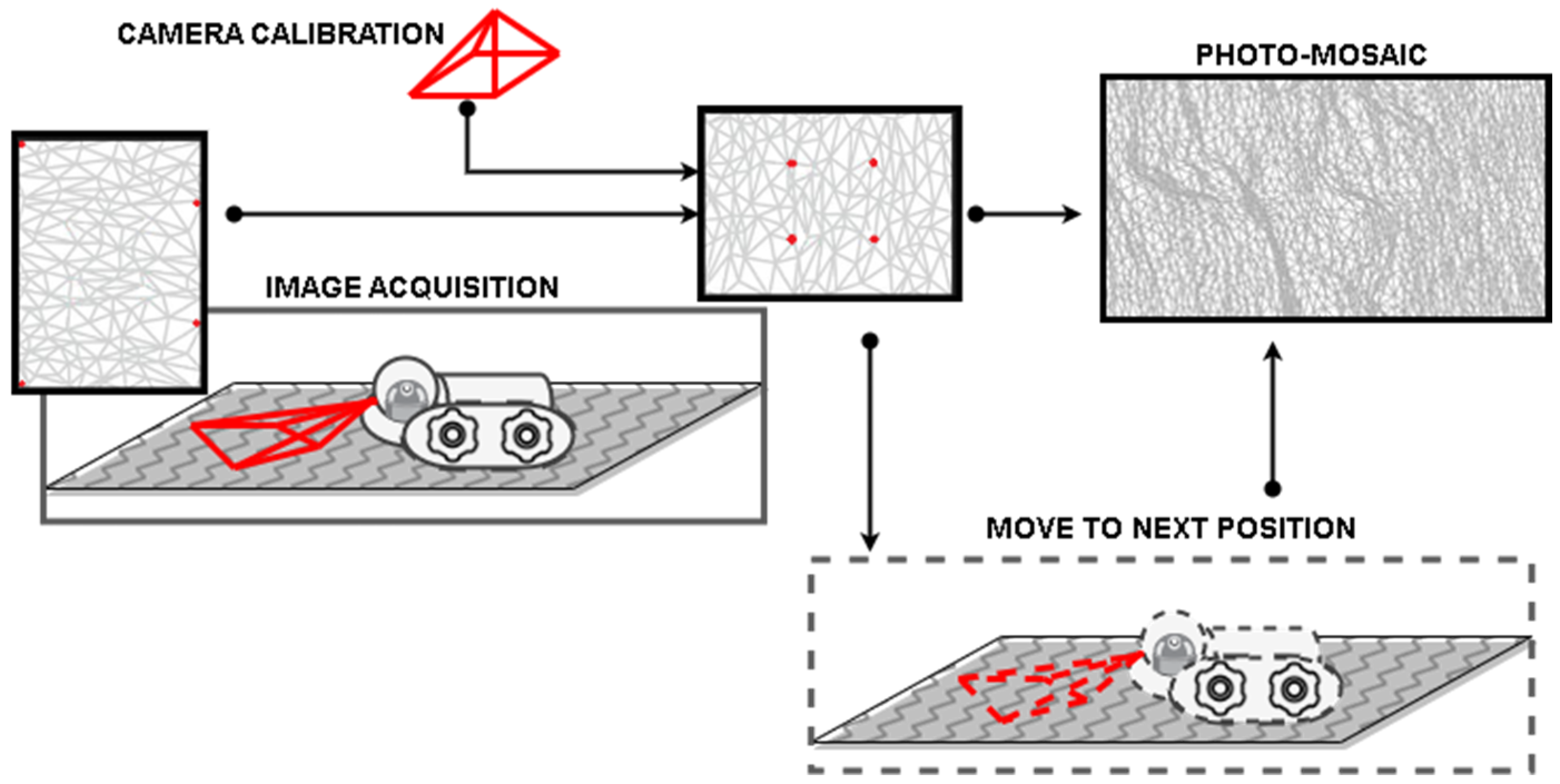
2.4. Image Acquisition for Automated Photo-Mosaics

A relevant aspect of ecological monitoring is the capability to extract 360º photo-mosaic panoramas for specific transect stations [58,59]. The scale of the photo-mosaics allows for the visualisation of changes in spatial patterns and processes in the studied landscape, with a focus on cartography to follow the changes in the timescale. Accordingly, a photo-mosaic was created automatically, taking sequential photos from the crawler camera each time the mobile platform moved a step forward. To the best of the authors’ knowledge, there is no previous work or experience using crawlers for developing underwater automated photo-mosaics, and it represents a novelty to follow its improvement during future trials.

The Global Alignment (GA) uses any navigation data and acquired images to estimate different camera positions across the transect [60]. It is a fusion of parameters to find an order in the photo sequence and extract the points of interest between each image. At the same time, with the knowledge of the trajectory that occurs at the start, the GA is used to generate more accurate visual maps. Encompassing perspective transformation techniques, GA techniques, and other image fusion techniques, it results in a set of heterogeneously similar images with a uniform, continuous appearance, and a common frame of reference.

A major factor that causes difficulties is when there is a short distance between the background and the camera; this can lead to parallax problems affecting the 2D photo-mosaics. In particular, it arises when there is the assumption of a flat scene with deficiencies in the calculation of two-dimensional transformations.

The trajectory of the video-transects was programmed in a single forward direction with constant 50 W power in each motor. The displacement lasted 30 s.

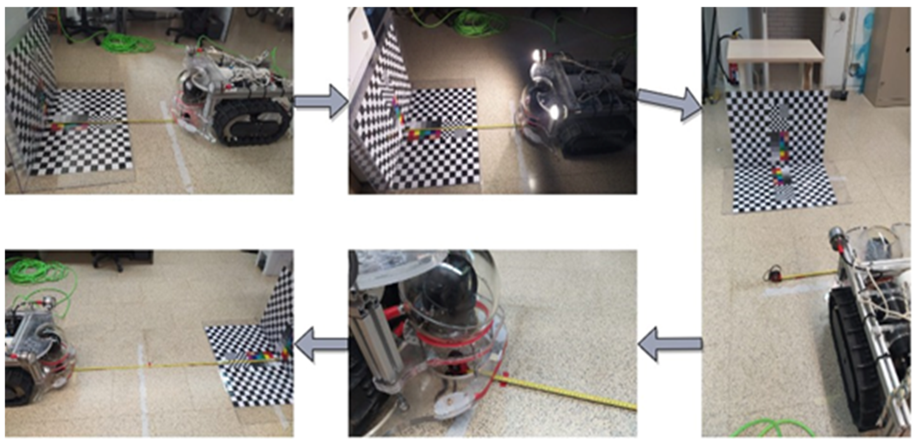
2.4.1. Camera Movement

The construction of the image set for mosaic composition has difficulties arising from environmental light changes or the computational expense involved in processing a voluminous data set. The first step is based on the theory that the area covered by each image is related to the altitude and the angle of the camera’s field of view. For this reason, before implementing such a photo-mosaic procedure on the crawler, a set of static tests was carried out with the camera located at different points in a room.

Then, the method of extraction and movement of the camera was analysed. A total of eight controls plus the central position (origin) were automatically recorded based on the specification of the Common Gateway Interface (CGI) Commands of API of SANTEC BW for the remote camera. The CGI command is used to fix the camera position in the defined places based on the horizontal and vertical position, and the predefined zoom is a PTZ control command with the following syntax: http://<username>:<password>@<ip>/cgi-bin/ptz.cgi?action=start&channel=0&code=Position&Horizontal position=[argstr]&Vertical position=[argstr]&Zoom change=[argstr]. A 360° movement was therefore achieved with three different angles, first at 15°, then at 30°, and finally at 45°. The vertical angle was always left constant, and the horizontal one was changed according to each angle. Then, each set acquired a different total number of images until the complete vision was reached.

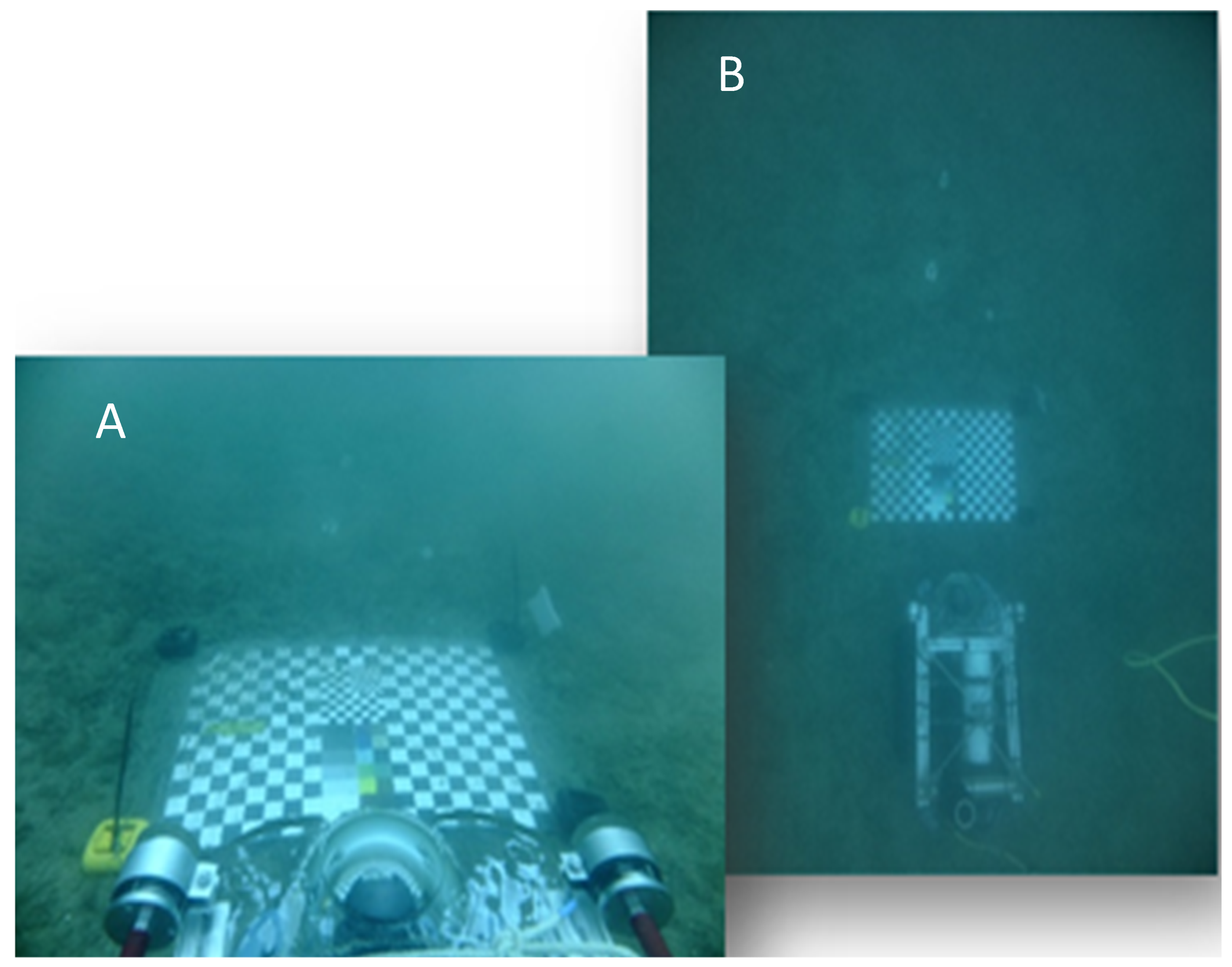
2.4.2. Camera Calibration

Some specific parameters were studied during the calibration process because of the intrinsic and extrinsic properties of the images. The intrinsic parameters include elements such as focal length, tilt coefficients, and optical centre, specific to each camera. In contrast, the extrinsic parameters refer to the translation that occurs between a point in real-world 3D space and the projection of a 2D coordinate (pixel), including rotation vectors. Consequently, the internal configurations are common in all captured images, in contrast to the external ones being different for each one.

The calibration of the image was required to avoid alterations typical of the marine medium, such as the optical properties and illumination conditions of water, severely affecting the underwater imagery [61]. Firstly, there is light attenuation and scattering (for differential wavelength absorption by the water and dissolved particles) which imparts a noticeable effect on the reproduction of the real colour and the range of visibility.

Secondly, a short focal length was used to obtain a wider view. Consequently, the most common distortion in these cases is the barrel type (i.e., the coordinates of the image move away from their original position) and this can generate the incorrect identification of species and other marine objects. Therefore, the calibration was based on the physics of ray maps (Figure 7) and we calibrated the cameras with the help of an object of known dimensions that is put underwater in situ [62]. We used an image made of frames with pixels of different sizes and colours, in order to provide a series of specific points, linking the radial distortion as pixel displacement along the same axis. During this calibration step, we took 10 images of the board from different angles.

Accuracy relies on the quantification of the radial distortion as the displacement of pixels along the same axis [63]. Regarding the FOV expansion in water, the effect is the same as when the camera approaches the area of interest, demonstrating large 3D distortions. Therefore, accuracy relies on the search for the coordinates in the image corresponding to the object. The following procedure is based on finding the 2D points on the board with the 10 images loaded. The 3D location of the points, and the 2D pixel position of the corners, were identified and extracted. To conclude, the process ends with the correction of the images. It is about delineating 3D points from real-world coordinates and their 2D locations. The calibration in the real marine environment, therefore, was performed at the OBSEA as shown in Figure 8.

2.4.3. Images Vertical Transformation and Spatial Collation

The quality of a photo-mosaic is conditioned by the good resolution and the optimal and lateral overlapping of the images. The features to consider are the altitude, the speed when making the transects, and the space between captures. Two relevant concepts related to each other are the term “overlap” and points of interest. The former takes advantage of the common area between two sequential images along a line. Differently, the points of interest are elements such as margins, corners, and objects that are used to identify the features of each image and find the common points to carry out the mixing. These are detected through autocorrelation methods and a “label” or unique value is applied. In that manner, when two images with the same label match, the position, rotation, and scale of the next one are directly calculated to make the last mixing step.

Finally, to avoid the double appearance of objects or the difficulty of discovering points of interest, it is necessary to choose a narrow transition area, when high-frequency and larger-scale elements appear, and a wider area, when there are not enough joining points, to have a correct smoothing technique. The intensity of the resulting pixels of each image is determined through a weighted average of the overlapping images and removes the barrier between the two images and yields a smooth effect. All these high-intensity features are reduced by a process called “blending”.

The vertical transformation is the relocation of points according to our reference system, resulting in the transformation of an area in the shape of a trapezoid (in our study) to a second square. What is necessary is to disturb the not visible parallel lines of each image in the vertical axis to have a change of perspective. The method has five transformation frames: the coordinates of the object, those of the real world, and those of the camera in 3D, and the situation of the image plane and the pixels that compose it in 2D. At the same time, once the images are calibrated, the generated code is implemented according to the requirements of the new projection, that is, the correction of the rotation angle according to the 2D points of the real world, the application of the extrinsic parameters, the position of the new camera coordinates with their intrinsic parameters, and the storage of the new images with 2D points.

An automated routine was developed in Python (Figure 9) referring to the pre-defined sequence used for the joining of images by comparing every two images one by one (i.e., by generating the loop joining of a 2 + 1 system, resulting in a panorama, and adding the next, consecutively). The main body of the code is based on various functions for detecting matches between photographs, generating matrices, fixing axes, and defining initial and new coordinates. A bilinear interpolation is performed by clipping the automatically originated black margins but leaving the deviation between images on a black background to visualise the created displacement. Finally, the last step of unifying in a single photo-mosaic with cylindrical projection is performed.

2.5. The Validation of Crawler Ecological Monitoring Efficiency

A total of 120 images of an estimated FOV volume equal to 10.5 m³ were acquired by the OBSEA fixed camera at a 30 min time-lapsed frequency. Images were taken during the week before but not at the time of the deployment of the crawler, i.e., 23–28 November 2021. The reason for this is that divers’ presence and operations can affect fish behaviour (i.e., attraction or repulsion) and bias species detections in the video census [64,65]. On the other hand, the crawler’s video footage had a total duration of 15 min and covered an estimated FOV of 243 m³ (i.e., the total volume of the water column visualised during the transect).

The computing of rarefaction curves was carried out to compare the efficiency of the crawler and the OBSEA camera surveys via the computing of two commonly used indices: Richness and Coleman’s rarefaction [66,67]. Assigning a concrete timestamp to each fish individual in the crawler’s footage was challenging within the scope of this demonstration, therefore we decided to create a simulated time series based on the total fish counts. As the crawler’s footage was only 15-min long, there was no expected periodicity in the fish counts to construct the rarefaction curve. Thus, we divided the video into 90–10 s long segments, and fish appearances for each species were treated as homogeneous Poisson processes with an expected rate λ, constant for all segments, and equal to the mean counts per segment. For each species, 100,000 time series were simulated based on the corresponding Poisson rate, with the median abundance coinciding with the reported one. Then, one of the simulated time series was randomly selected to create the input table for the rarefaction curves. Simulations were performed with the R statistical software [68]. The rarefaction analysis was performed with the software EstimateS 9.1 [69].

3. Results

This section includes the following parts: Section 3.1: the testing of the crawler components; Section 3.2: the validation of crawler driving functionalities; Section 3.3: the automatically generated photo-mosaic; and, finally, Section 3.4: the outcomes of crawler video-monitoring efficiency.

3.1. The Testing of the Crawler Components

The crawler and all its components were tested in three progressive phases (Figure 10). Firstly, the crawler was tested in a hyperbaric chamber to simulate the water pressure (i.e., depth) resistance. In this step, we used 2.5 bars of pressure, simulating the maximum depth of 25 m (Figure 10A).

Then, the first series of driving tests were conducted in a swimming pool facility of the SARTI-UPC laboratory (Figure 10B) to validate buoyancy and movement. One central aspect was to achieve the correct balance through buoyancy which was evaluated during a total of 6 h of driving trials. The observations during this test revealed the need for an additional weight of 4 kg for crawler stability to compensate for the positive buoyancy of the camera’s sphere (this stability was validated during the second deployment of the crawler in the OBSEA observatory area for 2 weeks).

Finally, the crawler was deployed at the OBSEA site and, connected by SCUBA divers, to the observatory junction box through its Ethernet cable (Figure 10C). At this step, the crawler was remotely navigated by an accredited user while the recorded videos were uploaded and stored online. An example of a video frame is reported in Figure 10D, along with the timestamp coordinates of its acquisition.

3.2. The Validation of Crawler Driving Functionalities

Validation of the crawler’s automatic driving mode was carried out (Figure 11). In brief, a 16 m² squared dive trajectory was planned near the OBSEA area, and four white plastic tags were placed as marks of the square’s vertices: opposite square’s vertices are marked with circular (Figure 11A,B) or rhomboid (Figure 11C,D) plastic tags. Then, by using the automatic control mode, the crawler was sent out to reach each one of these marks. A summary of those tests is visible online (https://www.youtube.com/watch?v=2ZltALzNnKA, accessed on 18 April 2023). In this video, achieved with the Sofar Trident (OpenROV) [70], we first presented how the crawler was deployed and connected to the OBSEA junction box. Then, the movement of the crawler was filmed along the established path, taking care to video-record its approach to the designated tags. Meanwhile, the crawler was filming the outer environment and transmitting the video to the website by using the OBSEA’s fibre optic network. This video can be seen from the operator console at the land station in real time at a minimum frame rate of 10 frames per second at full resolution. This video is also stored on a “Raspberry Pi” in order to be processed by the auto photo-mosaic algorithm (see Section 3.3). On the public website, the resolution of video and frame rate may be reduced by the available internet bandwidth.

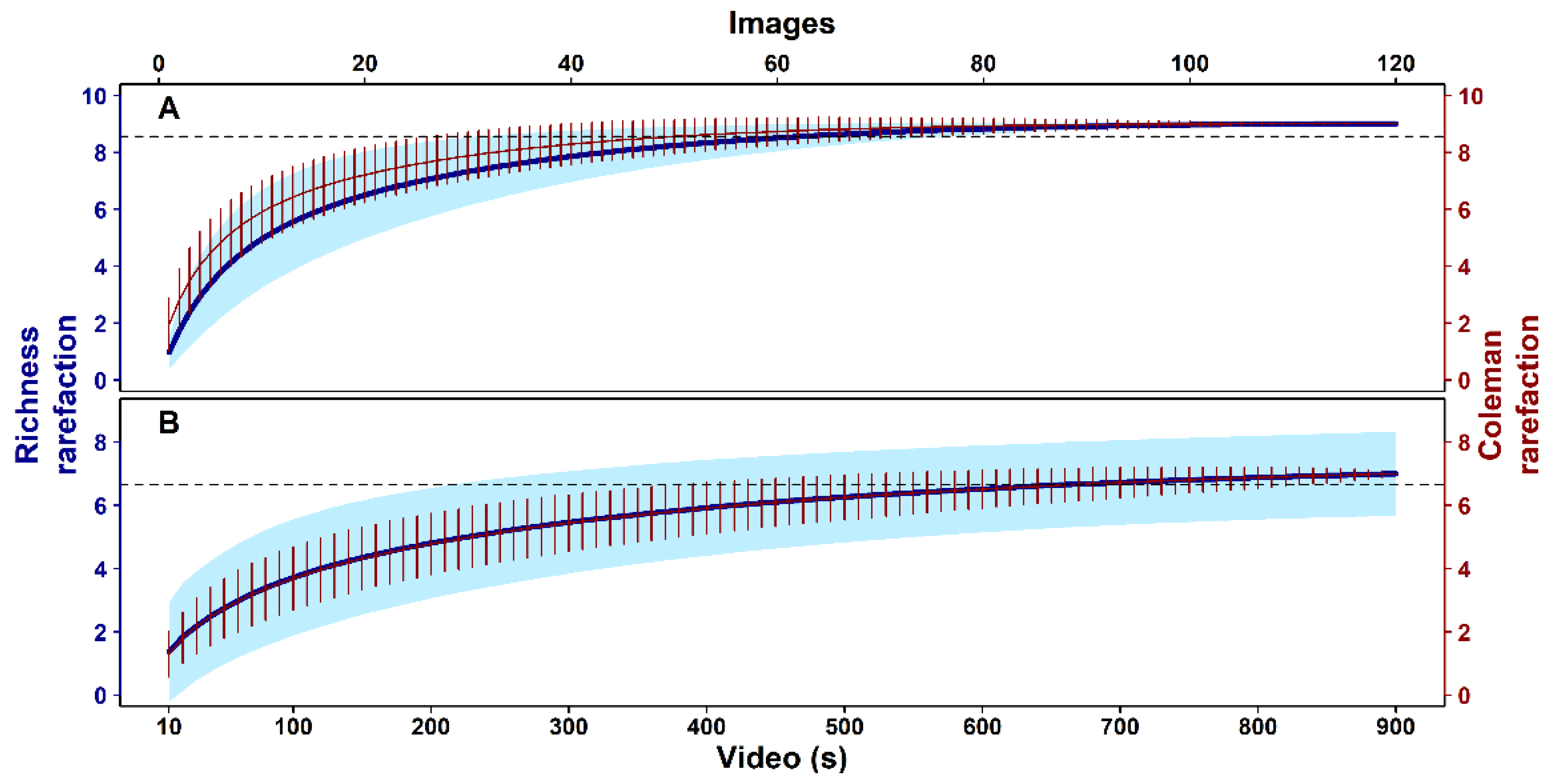
3.3. Extension of the Monitoring Radius and Outcomes of Crawler Video-Monitoring Efficiency

The limited monitoring domain of the OBSEA observatory was expanded to a 40 m radius by adding the underwater crawler (Figure 12). The crawler was connected to the OBSEA observatory by a 50 m long cable and, thus, increased the monitoring domain. This radius could be further increased by connecting the crawler with a longer cable.

With this expansion, different quantities and individuality of species from the camera of OBSEA were observed. Then, the identification and classification of individual fish were carried out manually by a trained operator following FishBase [71]. A total of 487 and 207 fish individuals (corresponding to nine and seven species, including a family and various unidentified taxa) were counted from the OBSEA camera images and the crawler’s footage, respectively (

Table 2. The number of individuals for each taxon (and densities per m³ in parentheses) as identified with the OBSEA and crawler cameras during the testing period. OTU refers to visible but not classified individuals.

	OBSEA	Crawler
Chromis chromis	350 (11.111)	163 (0.671)
Coris julis	0	23 (0.095)
Dentex dentex	17 (0.54)	0
Diplodus cervinus	3 (0.095)	0
Diplodus spp.	7 (0.222)	0
Labridae	0	10 (0.041)
Seriola dumerili	7 (0.222)	0
Serranus cabrilla	0	1 (0.004)
OTU 1	46 (1.460)	3 (0.012)
OTU 2	33 (1.048)	0
OTU 3	3 (0.095)	0
OTU 4	21 (0.667)	0
OTU 5	0	5 (0.021)
OTU 6	0	2 (0.008)
Total	487 (15.460)	207 (0.852)

). The fish Chromis chromis and an unidentified fish Operational Taxonomic Unit (OTU), as distant within the FOV or not aligned (hence being not assigned to any specific taxonomic level), were common in the imaging material obtained from the two sources.

The rarefaction analysis (Figure 13) showed that the curve for the fixed camera reached a plateau, while the one for the crawler continued to ascend until the end of the progressively added samples (i.e., video segments). According to that analysis, in order to record at least 95% of the species present in the area during the respective study period, we would need more than 700 s of video footage from the crawler camera.

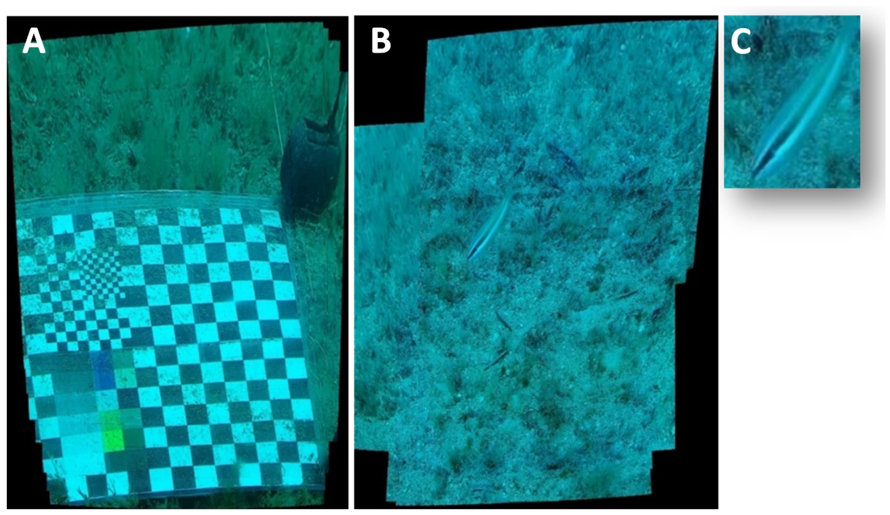
3.4. The Automatically Generated Photo-Mosaics

The auto photo-mosaic was conducted in the shore station on an online Raspberry Pi 4 embedded system. Each second a photo was taken and the time for the algorithm to make auto photo-mosaic was less than 200 ms. As an example, a limited field of view of one minute of transects is shown below (Figure 14). In this figure, we reported the checkerboard photo-mosaic generated after the calibration on the left image and the detection of a fish from a second photo-mosaic on the right image.

4. Discussion

In this paper, we described the assemblage and testing of a small coastal crawler added to the OBSEA cabled observatory which extends the current (semi)automated crawler monitoring capabilities drastically when compared to current state-of-the-art crawlers such as the Rossia, Wally, and Norppa crawlers. We described its assemblage and testing at the OBSEA cabled observatory, providing details on its web management architecture, navigation capability, video monitoring performance, and overall costs. Below, we discuss the main technological challenges we faced during the construction, deployment, and testing process, as well as the validation of the crawler video data for ecological monitoring. This latter is an operationally key aspect for the inclusion of the developed crawler and other mobile platforms such as docked AUVs within future cabled observatory monitoring practices, for which the OBSEA is paradigmatic as EMSO Test-Site.

4.1. Technological Challenges during the Construction, Deployment, and Testing Process

The developed crawler prototype was assembled for shallow water operations. Accordingly, the test-site specifications have multiple effects on the structural design and energy provision of the assembled platform when compared to other operationally established deep-sea crawler versions such as “Wally” (i.e., deployed at an 870 m depth in a hydrocarbon seep area of the Barkley Canyon of the Canadian Pacific, by ONC [72]). Firstly, the shallow depth rating of the housing of our coastal crawler can vary in material type and dimensions. Despite the fact that its usage is limited to coastal ranges (i.e., max of 25 m depth), some of its components could withstand higher depth pressures of around 100 m (i.e., the junction box cylinder, oil-filled motors, and camera sphere glass housing). Here, we used a Plexiglas chassis instead of titanium, with consistent hand manoeuvrability, due to the reduction in weight and overall size/volume (i.e., from ~1 m³ of Wally to ~0.22 m³ of OBSEA Crawler).

Secondly, the site receives natural illumination during a part of the 24-h cycle (i.e., the OBSEA infrastructure is deployed at only a 20 m depth). Even during the night-time, there is still some moonlight penetration, in contrast to the complete darkness of the deep-sea [73]. This remark is of relevance in the evaluation of the platform energy expenditure. The 8 W lights of this coastal crawler are sufficient to allow navigation and video-monitoring operations at night-time, in contrast to the 33 W lights required by its deep-sea rated equivalent, “Wally” [41]. This represents a consistent power consumption reduction, to be taken into account for platform development, related to operational energy autonomy under a future scenario of untethering (see Section 4.3).

Thirdly, we had to face problems with navigation assets and cable abrasion in a high- hydrodynamic coastal environment. The current system of our coastal deployment area is higher than that of the deep-sea hydrates site, where the crawler “Wally” is operating. Waves, storms, and surface circulation can exceed 0.9 m/s at the OBSEA site [74,75,76], whereas deep-sea inertial currents, benthic storms, and convection currents, usually reach more moderate velocities up to 0.6 m/s [77,78,79]. To overcome this challenge, the floating characteristics of the cable were considered to avoid drag, which would slow down the crawler (e.g., platform entanglement) and create concerns for the cable itself, as in the case of abrasion. To address this issue, we added foam floaters (i.e., 190 mm in diameter and buoyancy of 1800 g) at equidistant spaces to make the cable neutrally (or slightly positive) buoyant.

In

Table 3. Comparing different features of the OBSEA crawler, with the Wally, Rossia, and Norppa crawlers.

Category	Specifications	OBSEA Crawler	Wally	Rossia	Norppa
Ecosystem Domain	Depth Rating (m)	Coastal (50)	Deep-sea (6000)	Deep-sea (3000)	Deep-sea (300)
Technical Specifications	Dimensions LWH (cm)	100 × 55 × 40	129 × 106 × 89	140 × 100 × 85	150 × 110 × 95
	Weight in air (kg)	56	303	280	350
	Motors	Faulhaber Brushless DC; 126 W, 12,800 rpm	Dunker Brushless DC; 600 W, 3370 rpm	Dunker Brushless DC; 600 W, 3370 rpm	Dunker Brushless DC; 600 W, 3370 rpm
Operational Capacity	Payload	Camera, 2 × 4 W LEDs (able to carry CTD, ACDP, second camera, acoustic modem, and USBL)	2 × cameras, laser scanner on PT unit, CTD, ADCP, fluorescence and turbidity meter, methane and oxygen sensors, and 3 × 33 W LEDs	2 × cameras, laser scanner on PT unit, CTD, ADCP, fluorescence and turbidity meter, methane and oxygen sensors, 3 × 33 W LEDs, and benthic chamber	2 × cameras, sonar, electromagnetics, CTD, and UXO sensor
	Manipulator	N	N	On-demand	Y
	Data Products	Imaging, video, and auto photo-mosaics	Imaging, video, photo-mosaics, 3D-point clouds, and environmental	Imaging, video, photo-mosaics, 3D-point clouds, environmental, and physical sampling	Imaging, video, sonar, electromagnetics, environmental, TNT explosives, and chemistry
Autonomy	Mission Control	Tethered, operated in real time/pre- programmed; hybrid (GUI and/or command- based) control; three locomotion modes (straight, turn, and rotate)	Tethered, operated in real time; hybrid (GUI and/or command- based) control; three locomotion modes (straight, turn, and rotate)	Tethered/ surface buoy/ autonomous, operated in real time/pre- programmed; GUI-based control; three locomotion modes (straight, turn, and rotate)	Tethered/ surface buoy/ autonomous, operated in real time/pre- programmed; ROS2 operating system; three locomotion modes (straight, turn, and rotate) with obstacle avoidance
	Power Consumption (W)	172.5 (at 100% motor power)	800 (at 100% motor power)	800 (at 100% motor power)	1000 (at 100% motor power)
	Cost (EUR)	28,000	150,000	320,000	400,000

, different features of the OBSEA coastal crawler, compared with the deep-sea Wally, Rossia, and Norppa crawlers are shown. As it is shown in the table, the advantage of the OBSEA crawler over other crawlers in terms of energy consumption and costs is obvious. In addition, the OBSEA underwater crawler is capable of automated photo-mosaic composition and is able to support the same instruments that other deep-sea crawlers can carry.

Regarding control and navigation, the presence of different modes enables fine-tuning the crawler’s response to fit the needs of the different missions. For instance, the option to switch to the manual mode allows controlling the fine movement of the crawler. This capability is important in order to focus, for example, on specific, fine-scale features of the seabed (or slow-moving epibenthic animal) as sentinel sites. Those sites need to be revisited in order to achieve an understanding of the ongoing ecological processes for the restoration or mitigation of impact strategies. Suitable metrics to be measured by a crawler could be, e.g., sessile organisms spanning from Posidonia meadows, clam fields, sponges, cold water corals, bryozoans, etc. [41,49,80]. On the other hand, the automatic mode allows for the repetition of pre-defined routines without the need for human intervention (e.g., back-and-forth time-lapse transects), when structural sampling is more significant than opportunistic observations. This would be the case for monitoring species’ habitat use in different contexts of different habitat heterogeneity and producing species counts and density data to be analysed by heat maps for each transect [47,48,81].

Ongoing tests are being performed to increase crawler functionalities in relation to its acoustical tracking by the nearby OBSEA platform. Deep-sea experiments are being conducted to enforce the platforms’ acoustic reciprocal communication [82,83] as well as the platforms’ capability to identify and follow acoustically tagged specimens and cooperating mobile platforms, e.g., ROVs and AUVs [84]. The acoustic tracking of individuals falls within the strategies of capturing and redeploying animals of commercially exploited species within strategic continental margin areas (e.g., fishery no-take zones), following their displacements as a source for geographic connectivity [85,86]. Future developments will refer to the installation of an acoustic modem (EvoLogics, S2C [87]) on the crawler and an Ultra-Short Base-Line (USBL, EvoLogics S2C) positioning system at the OBSEA observatory.

Another interesting future perspective is the incorporation of an Inertial Measurement Unit (IMU) instrument within the crawler structure in order to detect its exact positioning on an irregular field [88]. Furthermore, combining geolocalisation and obstacle detection systems is of great interest because it gives us the possibility to generate maps based on localisations using a “Simultaneous Localization and Mapping” (SLAM) system [89]. Therefore, with the SLAM navigation help, the crawler itself will be able to generate visual maps of the seabed via photo-mosaic procedures.

4.2. The Validation of the Crawler Video Data for Ecological Monitoring

The footage of the crawler’s field test was compared to the imaging output of the fixed time-lapse camera of the OBSEA, as captured during the week prior to the crawler’s deployment.

This comparison served a dual purpose: first, to assess if imaging transects with the crawler can successfully depict a comparable portion of the biodiversity identified via the OBSEA’s fixed camera; and second, to highlight the complementary nature of the two monitoring platforms due to their unique characteristics (see below).

Time-lapse imaging depicted more species and taxonomic units (i.e., higher richness) in comparison to the crawler (i.e., nine vs. seven). Nevertheless, the rarefaction curve with the crawler’s data did not reach the plateau phase (see Figure 13), indicating that more species would be present in longer or more temporally diverse videos. The fact that the confidence interval band for the crawler did not become narrower after the integration of all samples supports this assumption. It should also be noted that the quality of the crawler’s camera is higher than that of the OBSEA, which influences the identification and classification of the fish individuals.

In regard to community composition, only two species were present in the material from both sources. This may reflect an operational distinction, in that the crawler footage focused mainly on the epibenthos, while the OBSEA camera imaging focused on the pelagic environment. On the other hand, the fixed camera’s imaging regime encompassed multiple 24-h cycles, while the crawler operated within a short interval in the mid-morning hours, potentially missing any species with potentially nocturnal activity patterns (e.g., [90,91]). Finally, the presence of the fixed structure can act as an artificial reef within the OBSEA camera-spanned area but not the crawler’s FOV, which may provoke higher species counts for the attraction of more individuals [92]. In any case, these preliminary results are indicative of the high complementarity of the two monitoring platforms, and the potential to expand the ecological representativeness of the entire network in space and time towards a four-dimensional, ecosystem-based monitoring protocol.

Furthermore, by using the outcomes from the procedures carried out to generate a photo-mosaic of the images acquired from the crawler, important future perspectives can be foreseen. In particular, an automatic system for detecting objects and, above all, species is still in the process of being tested. From these tests, we want to generate a system able to detect and classify marine animals [93,94]. At the same time, we want to create an automatic obstacle avoidance system [95,96]. In other words, we want to build a system that positions the different elements in the FOV of the crawler camera in the different space-time scales to automatically detect specimens and track them.

4.3. Scientific and Operational Impact

Sampling marine biodiversity at relevant spatiotemporal scales is of strategic interest in management and conservation policies and has to be able to acquire biological data considering the local habitat heterogeneity of the managed areas (e.g., marine protected areas and fishery no-take zones). At the same time, it must meet repetition requirements at the diel and seasonal scales to portray species counts variations as a product of activity rhythms (i.e., resulting in massive population displacements) [20,97,98]. Therefore, the implementation of economically affordable and smart-monitoring technology, easy to deploy from any opportunity vessel, is of pivotal importance.

A promising example is represented by the newly developed teleoperated crawlers used by marine scientists to carry out multiparametric environmental studies via time-lapse imaging or video transects, accompanied by a diversified set of oceanographic and geochemical sensors [47,81,99]. The advanced crawler model for deep-sea operations, such as the Wally mobile platform, has evolved into the new “Rossia” platform [100], which presently costs EUR 150,000 with no installed sensor payload, but is capable of full operational autonomy (untethering). We could efficiently produce a shallow water prototype version whose total price stays around EUR 20,000, a price contained due to the lack of high depth-rated restrictions in the preparation of the components.

The crawler can be teleoperated via a fibre-optics 50 m length and buoyant tether, making it a highly versatile solution, as it allows operations in both urban areas around piers and docks as well as in distant zones thanks to its coupling with the autonomous cabled observatories. The compact size/weight specifications of our prototype favour the handling/transporting with opportunity vessels, and this opens up the possibility for its connection to landers as benthic multiparametric and autonomous workstations.

In coastal areas, video crawlers have the advantage of replicating human-based monitoring techniques (underwater visual census by SCUBA divers; e.g., [98,101]) in a more spatiotemporal intensive fashion; human-based monitoring is not often repeated at day-night frequencies [102]. Video census transects, equivalent to what would be achieved by a human operator, could be even expanded, by widening the FOV, whenever panoramic sweeps can be taken at different stations [98]. This procedure would allow for the spatial scale of the local representation power of ecological data to be acquired by fixed observatory cameras in larger areas, as could be achieved by trawl hauling.

Therefore, the elaborated crawler prototype could be of value for fishery-independent and video-based stock assessment routines when focussing on commercially relevant species [103]. With this new coastal prototype, transects can be repeated back and forth over specific video pathways, to conduct fish counting over 24-h. With the addition of a pair of scaling lasers (as those used by ROVs), a video-inspected area can be computed. This upgrade would allow for establishing a transition in the ecological quality of acquired data [104] from mere counts to more demographic-oriented population density estimates. The developing network of cameras at the OBSEA, two fixed (i.e., OBSEA and tripod cameras) and one mobile (i.e., crawler), will allow us to have more representative data on the abundance and biodiversity of the local communities, increasing the video monitored area [105]. This sampling could be repeated at an hourly frequency over consecutive months with a reduced cost, providing also more representative data on the behaviour of the local fauna [106].

At the same time, advances in the field of operational autonomy (e.g., energy provision and smart navigation) and data processing through artificial intelligence routines, will be valuable assets for deployments in diverse coastal areas [94]. The use of landers for faunal abundance, behaviour, and biodiversity characterisation dates back more than four decades (e.g., [107]). In the near future, more economically affordable landers (compared to cabled observatories) will be available. Easily redeployed landers plus their own docked crawler (via the expansion of a specific docking station) will be used to operate in targeted marine areas over prolonged periods of time with no retrieval [100].

5. Conclusions

In this paper, we showed how to implement and adapt a coastal crawler to drastically extend its ecological monitoring capability in synchronisation with a fixed-cabled observatory such as the OBSEA. The hardware and software components and functionalities described here can serve as a benchmark for the development of similar tools in other coastal cabled observatories of the EMSO network and beyond (i.e., other oceanic infrastructures). In the future, low-cost mobile platforms of this kind may contribute substantially to extending the spatiotemporal dimensions of our remote, vessel, and human-independent monitoring capabilities.

References

1. Costa, C.; Fanelli, E.; Marini, S.; Danovaro, R.; Aguzzi, J. Global Deep-Sea Biodiversity Research Trends Highlighted by Science Mapping Approach. Front. Mar. Sci. 2020, 7, 384. [Google Scholar] [CrossRef]
2. Barnes, C.R.; Tunnicliffe, V. Building the World’s First Multi-Node Cabled Ocean Observatories (NEPTUNE Canada and VENUS, Canada): Science, Realities, Challenges and Opportunities. In Proceedings of the OCEANS 2008-MTS/IEEE Kobe Techno-Ocean, Kobe, Japan, 8–11 April 2008. [Google Scholar] [CrossRef]
3. Favali, P.; Beranzoli, L. Seafloor Observatory Science: A Review. Ann. Geophys. 2006, 49, 515–567. [Google Scholar] [CrossRef]
4. Barnes, C.R.; Best, M.M.R.; Johnson, F.R.; Pautet, L.; Pirenne, B. Erratum: Challenges, Benefits, and Opportunities in Installing and Operating Cabled Ocean Observatories: Perspectives from NEPTUNE Canada (IEEE Journal of Oceanic Engineering (2013) 38:1 (144–157)). IEEE J. Ocean. Eng. 2013, 38, 406. [Google Scholar] [CrossRef]
5. Aguzzi, J.; Chatzievangelou, D.; Marini, S.; Fanelli, E.; Danovaro, R.; Flögel, S.; Lebris, N.; Juanes, F.; De Leo, F.C.; Del Rio, J.; et al. New High-Tech Flexible Networks for the Monitoring of Deep-Sea Ecosystems. Environ. Sci. Technol. 2019, 53, 6616–6631. [Google Scholar] [CrossRef]
6. Grinyó, J.; Francescangeli, M.; Santín, A.; Ercilla, G.; Estrada, F.; Mecho, A.; Fanelli, E.; Costa, C.; Danovaro, R.; Company, J.B.; et al. Megafaunal Assemblages in Deep-Sea Ecosystems of the Gulf of Cadiz, Northeast Atlantic Ocean. Deep Sea Res. Part I Oceanogr. Res. Pap. 2022, 183, 103738. [Google Scholar] [CrossRef]
7. Dodge, K.L.; Kukulya, A.L.; Burke, E.; Baumgartner, M.F. TurtleCam: A “Smart” Autonomous Underwater Vehicle for Investigating Behaviors and Habitats of Sea Turtles. Front. Mar. Sci. 2018, 5, 90. [Google Scholar] [CrossRef]
8. Veitch, E.; Alsos, O.A. Human-Centered Explainable Artificial Intelligence for Marine Autonomous Surface Vehicles. J. Mar. Sci. Eng. 2021, 9, 1227. [Google Scholar] [CrossRef]
9. Wu, G.; Lu, Z.; Luo, Z.; Shang, J.; Sun, C.; Zhu, Y. Experimental Analysis of a Novel Adaptively Counter-Rotating Wave Energy Converter for Powering Drifters. J. Mar. Sci. Eng. 2019, 7, 171. [Google Scholar] [CrossRef]
10. Aguzzi, J.; Costa, C.; Calisti, M.; Funari, V.; Stefanni, S.; Danovaro, R.; Gomes, H.I.; Vecchi, F.; Dartnell, L.R.; Weiss, P.; et al. Research Trends and Future Perspectives in Marine Biomimicking Robotics. Sensors 2021, 21, 3778. [Google Scholar] [CrossRef]
11. Danovaro, B.R.; Aguzzi, J.; Fanelli, E.; Smith, C.R. An Ecosystem-Based Deep-Ocean Strategy. Science 2017, 355, 452–454. [Google Scholar] [CrossRef]
12. Glaviano, F.; Esposito, R.; Di Cosmo, A.; Esposito, F.; Gerevini, L.; Ria, A.; Molinara, M.; Bruschi, P.; Costantini, M.; Zupo, V. Management and Sustainable Exploitation of Marine Environments through Smart Monitoring and Automation. J. Mar. Sci. Eng. 2022, 10, 297. [Google Scholar] [CrossRef]
13. Juniper, S.K.; Matabos, M.; Mihály, S.; Ajayamohan, R.S.; Gervais, F.; Bui, A.O.V. A Year in Barkley Canyon: A Time-Series Observatory Study of Mid-Slope Benthos and Habitat Dynamics Using the NEPTUNE Canada Network. Deep Sea Res. Part II Top. Stud. Oceanogr. 2013, 92, 114–123. [Google Scholar] [CrossRef]
14. Robison, B.H.; Reisenbichler, K.R.; Sherlock, R.E. The Coevolution of Midwater Research and ROV Technology at MBARI. Oceanography 2017, 30, 26–37. [Google Scholar] [CrossRef]
15. Bicknell, A.W.J.; Godley, B.J.; Sheehan, E.V.; Votier, S.C.; Witt, M.J. Camera Technology for Monitoring Marine Biodiversity and Human Impact. Front. Ecol. Environ. 2016, 14, 424–432. [Google Scholar] [CrossRef]
16. Canonico, G.; Buttigieg, P.L.; Montes, E.; Muller-Karger, F.E.; Stepien, C.; Wright, D.; Benson, A.; Helmuth, B.; Costello, M.; Sousa-Pinto, I.; et al. Global Observational Needs and Resources for Marine Biodiversity. Front. Mar. Sci. 2019, 6, 367. [Google Scholar] [CrossRef]
17. Mellin, C.; Parrott, L.; Andréfouët, S.; Bradshaw, C.J.A.; MacNeil, M.A.; Caley, M.J. Multi-Scale Marine Biodiversity Patterns Inferred Efficiently from Habitat Image Processing. Ecol. Appl. 2012, 22, 792–803. [Google Scholar] [CrossRef]
18. Mallet, D.; Pelletier, D. Underwater Video Techniques for Observing Coastal Marine Biodiversity: A Review of Sixty Years of Publications (1952–2012). Fish. Res. 2014, 154, 44–62. [Google Scholar] [CrossRef]
19. Aguzzi, J.; Iveša, N.; Gelli, M.; Costa, C.; Gavrilovic, A.; Cukrov, N.; Cukrov, M.; Cukrov, N.; Omanovic, D.; Štifanić, M.; et al. Ecological Video Monitoring of Marine Protected Areas by Underwater Cabled Surveillance Cameras. Mar. Policy 2020, 119, 104052. [Google Scholar] [CrossRef]
20. Aguzzi, J.; Chatzievangelou, D.; Company, J.B.; Thomsen, L.; Marini, S.; Bonofiglio, F.; Juanes, F.; Rountree, R.; Berry, A.; Chumbinho, R.; et al. The Potential of Video Imagery from Worldwide Cabled Observatory Networks to Provide Information Supporting Fish-Stock and Biodiversity Assessment. ICES J. Mar. Sci. 2020, 77, 2396–2410. [Google Scholar] [CrossRef]
21. Brandt, A.; Gutt, J.; Hildebrandt, M.; Pawlowski, J.; Schwendner, J.; Soltwedel, T.; Thomsen, L. Cutting the Umbilical: New Technological Perspectives in Benthic Deep-Sea Research. J. Mar. Sci. Eng. 2016, 4, 36. [Google Scholar] [CrossRef]
22. Ayma, A.; Aguzzi, J.; Canals, M.; Lastras, G.; Bahamon, N.; Mecho, A.; Company, J.B. Comparison between ROV Video and Agassiz Trawl Methods for Sampling Deep Water Fauna of Submarine Canyons in the Northwestern Mediterranean Sea with Observations on Behavioural Reactions of Target Species. Deep Sea Res. Part I Oceanogr. Res. Pap. 2016, 114, 149–159. [Google Scholar] [CrossRef]
23. Aguzzi, J.; Company, J.B. Chronobiology of Deep-Water Decapod Crustaceans on Continental Margins. In Advances in Marine Biology; Elsevier Ltd.: Amsterdam, The Netherlands, 2010; Volume 58, pp. 155–225. [Google Scholar]
24. Aguzzi, J.; Company, J.B.; Costa, C.; Menesatti, P.; Garcia, J.A.; Bahamon, N.; Puig, P.; Sarda, F. Activity Rhythms in the Deep-Sea: A Chronobiological Approach. Front. Biosci. 2011, 16, 131–150. [Google Scholar] [CrossRef] [PubMed]
25. Aguzzi, J.; López-Romero, D.; Marini, S.; Costa, C.; Berry, A.; Chumbinho, R.; Ciuffardi, T.; Fanelli, E.; Pieretti, N.; Del Río, J.; et al. Multiparametric Monitoring of Fish Activity Rhythms in an Atlantic Coastal Cabled Observatory. J. Mar. Syst. 2020, 212, 103424. [Google Scholar] [CrossRef]
26. Aguzzi, J.; Company, J.B.; Costa, C.; Matabos, M.; Azzurro, E.; Mánuel, A.; Menesatti, P.; Sardá, F.; Canals, M.; Delory, E.; et al. Challenges to the Assessment of Benthic Populations and Biodiversity as a Result of Rhythmic Behaviour: Video Solutions from Cabled Observatories. Oceanogr. Mar. Biol. Annu. Rev. 2012, 50, 235–286. [Google Scholar] [CrossRef]
27. Rountree, R.A.; Aguzzi, J.; Marini, S.; Fanelli, E.; De Leo, F.C.; del Río Fernandez, J.; Juanes, F. Towards an Optimal Design for Ecosystem-Level Ocean Observatories. In Oceanography and Marine Biology; Taylor & Francis: Abingdon, UK, 2020. [Google Scholar]
28. Cuvelier, D.; Legendre, P.; Laes, A.; Sarradin, P.M.; Sarrazin, J. Rhythms and Community Dynamics of a Hydrothermal Tubeworm Assemblage at Main Endeavour Field—A Multidisciplinary Deep-Sea Observatory Approach. PLoS ONE 2014, 9, e96924. [Google Scholar] [CrossRef]
29. Cristini, L.; Lampitt, R.S.; Cardin, V.; Delory, E.; Haugan, P.; O’Neill, N.; Petihakis, G.; Ruhl, H.A. Cost and Value of Multidisciplinary Fixed-Point Ocean Observatories. Mar. Policy 2016, 71, 138–146. [Google Scholar] [CrossRef]
30. Linley, T.D.; Craig, J.; Jamieson, A.J.; Priede, I.G. Bathyal and Abyssal Demersal Bait-Attending Fauna of the Eastern Mediterranean Sea. Mar. Biol. 2018, 165, 159. [Google Scholar] [CrossRef]
31. Priede, I.G.; Godbold, J.A.; King, N.J.; Collins, M.A.; Bailey, D.M.; Gordon, J.D.M. Deep-Sea Demersal Fish Species Richness in the Porcupine Seabight, NE Atlantic Ocean: Global and Regional Patterns. Mar. Ecol. 2010, 31, 247–260. [Google Scholar] [CrossRef]
32. Aguzzi, J.; Fanelli, E.; Ciuffardi, T.; Schirone, A.; De Leo, F.C.; Doya, C.; Kawato, M.; Miyazaki, M.; Furushima, Y.; Costa, C.; et al. Faunal Activity Rhythms Influencing Early Community Succession of an Implanted Whale Carcass Offshore Sagami Bay, Japan. Sci. Rep. 2018, 8, 11163. [Google Scholar] [CrossRef]
33. Aguzzi, J.; Chatzievangelou, D.; Francescangeli, M.; Marini, S.; Bonofiglio, F.; Del Rio, J.; Danovaro, R. The Hierarchic Treatment of Marine Ecological Information from Spatial Networks of Benthic Platforms. Sensors 2020, 20, 1751. [Google Scholar] [CrossRef]
34. Aguzzi, J.; Flögel, S.; Marini, S.; Thomsen, L.; Albiez, J.; Weiss, P.; Picardi, G.; Calisti, M.; Stefanni, S.; Mirimin, L.; et al. Developing Technological Synergies between Deep-Sea and Space Research. Elementa 2022, 10, 64. [Google Scholar] [CrossRef]
35. Johansson, B.; Siesjö, J.; Furuholmen, M. Seaeye Sabertooth A Hybrid AUV/ROV offshore system. In Proceedings of the OCEANS 2010 MTS/IEEE SEATTLE, Seattle, WA, USA, 20–23 September 2010; pp. 1–3. [Google Scholar] [CrossRef]
36. Chardard, Y.; Copros, T. Swimmer: Final Sea Demonstration of This Innovative Hybrid AUV/ROV System. In Proceedings of the 2002 Interntional Symposium on Underwater Technology, Tokyo, Japan, 19 April 2002. [Google Scholar] [CrossRef]
37. Zhang, Y.X.; Zhang, Q.F.; Zhang, A.Q.; Chen, J.; Li, X.; He, Z. Acoustics-Based Autonomous Docking for A Deep-Sea Resident ROV. China Ocean Eng. 2022, 36, 100–111. [Google Scholar] [CrossRef]
38. Podder, T.; Sibenac, M.; Bellingham, J. AUV Docking System for Sustainable Science Missions. In Proceedings of the IEEE International Conference on Robotics and Automation, New Orleans, LA, USA, 26 April–1 May 2004; pp. 4478–4485. [Google Scholar] [CrossRef]
39. Palomeras, N.; Vallicrosa, G.; Mallios, A.; Bosch, J.; Vidal, E.; Hurtos, N.; Carreras, M.; Ridao, P. AUV Homing and Docking for Remote Operations. Ocean Eng. 2018, 154, 106–120. [Google Scholar] [CrossRef]
40. Palomeras, N.; Peñalver, A.; Massot-Campos, M.; Vallicrosa, G.; Negre, P.L.; Fernández, J.J.; Ridao, P.; Sanz, P.J.; Oliver-Codina, G.; Palomer, A. I-AUV Docking and Intervention in a Subsea Panel. In Proceedings of the 2014 IEEE/RSJ International Conference on Intelligent Robots and Systems, Chicago, IL, USA, 14–18 September 2014; pp. 2279–2285. [Google Scholar] [CrossRef]
41. Purser, A.; Thomsen, L.; Barnes, C.; Best, M.; Chapman, R.; Hofbauer, M.; Menzel, M.; Wagner, H. Temporal and Spatial Benthic Data Collection via an Internet Operated Deep Sea Crawler. Methods Oceanogr. 2013, 5, 1–18. [Google Scholar] [CrossRef]
42. Xie, C.; Wang, L.; Yang, N.; Agee, C.; Chen, M.; Zheng, J.; Liu, J.; Chen, Y.; Xu, L.; Qu, Z.; et al. A Compact Design of Underwater Mining Vehicle for the Cobalt-Rich Crust with General Support Vessel Part A: Prototype and Tests. J. Mar. Sci. Eng. 2022, 10, 135. [Google Scholar] [CrossRef]
43. Raber, G.T.; Schill, S.R. Reef Rover: A Low-Cost Small Autonomous Unmanned Surface Vehicle (Usv) for Mapping and Monitoring Coral Reefs. Drones 2019, 3, 38. [Google Scholar] [CrossRef]
44. Picardi, G.; Chellapurath, M.; Iacoponi, S.; Stefanni, S.; Laschi, C.; Calisti, M. Bioinspired Underwater Legged Robot for Seabed Exploration with Low Environmental Disturbance. Sci. Robot. 2020, 5, eaaz1012. [Google Scholar] [CrossRef]
45. Chatzievangelou, D.; Aguzzi, J.; Scherwath, M.; Thomsen, L. Quality Control and Pre-Analysis Treatment of the Environmental Datasets Collected by an Internet Operated Deep-Sea Crawler during Its Entire 7-Year Long Deployment (2009–2016). Sensors 2020, 20, 2991. [Google Scholar] [CrossRef] [PubMed]
46. Flögel, S.; Ahrns, I.; Nuber, C.; Hildebrandt, M.; Duda, A.; Schwendner, J.; Wilde, D. A New Deep-Sea Crawler System—MANSIO-VIATOR. In Proceedings of the 2018 OCEANS—MTS/IEEE Kobe Techno-Oceans, OCEANS—Kobe 2018, Kobe, Japan, 28–31 May 2018; Institute of Electrical and Electronics Engineers Inc.: Piscataway, NJ, USA, 2018. [Google Scholar]
47. Doya, C.; Chatzievangelou, D.; Bahamon, N.; Purser, A.; De Leo, F.C.; Juniper, S.K.; Thomsen, L.; Aguzzi, J. Seasonal Monitoring of Deep-Sea Megabenthos in Barkley Canyon Cold Seep by Internet Operated Vehicle (IOV). PLoS ONE 2017, 12, e0176917. [Google Scholar] [CrossRef]
48. Chatzievangelou, D.; Aguzzi, J.; Ogston, A.; Suárez, A.; Thomsen, L. Visual Monitoring of Key Deep-Sea Megafauna with Internet Operated Crawlers as a Tool for Ecological Status Assessment. Prog. Oceanogr. 2020, 184, 102321. [Google Scholar] [CrossRef]
49. Chatzievangelou, D.; Thomsen, L.; Doya, C.; Purser, A.; Aguzzi, J. Transects in the Deep: Opportunities with Tele-Operated Resident Seafloor Robots. Front. Mar. Sci. 2022, 9, 833617. [Google Scholar] [CrossRef]
50. ONC Ocean Networks Canada. Available online: https://www.oceannetworks.ca/ (accessed on 1 October 2022).
51. Norppa Underwater Crawler. Available online: https://seaterra.de/web/UXO/start/index.php (accessed on 1 October 2022).
52. Aguzzi, J.; Mànuel, A.; Condal, F.; Guillén, J.; Nogueras, M.; del Rio, J.; Costa, C.; Menesatti, P.; Puig, P.; Sardà, F.; et al. The New Seafloor Observatory (OBSEA) for Remote and Long-Term Coastal Ecosystem Monitoring. Sensors 2011, 11, 5850–5872. [Google Scholar] [CrossRef] [PubMed]
53. Del-Rio, J.; Sarria, D.; Aguzzi, J.; Masmitja, I.; Carandell, M.; Olive, J.; Gomariz, S.; Santamaria, P.; Manuel Lazaro, A.; Nogueras, M.; et al. Obsea: A Decadal Balance for a Cabled Observatory Deployment. IEEE Access 2020, 8, 33163–33177. [Google Scholar] [CrossRef]
54. JERICO. Integrated Pan-European Multidisciplinary, and Multi-Platform Research Infrastructure Dedicated to a Holistic Appraisal of Coastal Marine System, C. Available online: https://www.jerico-ri.eu/ (accessed on 10 April 2021).
55. Molino, E.; Artero, C.; Nogueras, M.; Toma, D.M.; Sarria, D.; Cadena, J.; Río, J.; Manuel, A. Oceanographic Buoy Expands OBSEA Capabilities. In Fourth International Workshop on Marine Technology; Universitat Politècnica de Catalunya: Barcelona, Spain, 2011; pp. 3–5. [Google Scholar]
56. Christ, R.D.; Wernli, R.L. The ROV Manual: A User Guide for Observation Class Remotely Operated Vehicles; Butterworth-Heinemann: Oxford, UK, 2011; ISBN 9780750681483. [Google Scholar]
57. Wiki Odroid Website. Available online: https://wiki.odroid.com/odroid-c4/odroid-c4 (accessed on 12 March 2020).
58. Negahdaripour, S.; Xu, X. Mosaic-Based Positioning and Improved Motion-Estimation Methods for Automatic Navigation of Submersible Vehicles. IEEE J. Ocean. Eng. 2002, 27, 79–99. [Google Scholar] [CrossRef]
59. Firoozfam, P.; Negahdaripour, S. Multi-Camera Conical Imaging; Calibration and Robust 3-D Motion Estimation for ROV-Based Mapping and Positioning. Ocean. Conf. Rec. 2002, 3, 1595–1602. [Google Scholar] [CrossRef]
60. Campos, R.; Gracias, N.; Ridao, P. Underwater Multi-Vehicle Trajectory Alignment and Mapping Using Acoustic and Optical Constraints. Sensors 2016, 16, 387. [Google Scholar] [CrossRef]
61. Skarlatos, D.; Agrafiotis, P. Image-Based Underwater 3d Reconstruction for Cultural Heritage: From Image Collection to 3d. Critical Steps and Considerations. In Springer Series on Cultural Computing; Springer: Berlin/Heidelberg, Germany, 2020; pp. 141–158. [Google Scholar]
62. Georgopoulos, A.; Agrafiotis, P. Documentation of a Submerged Monument Using Improved Two Media Techniques. In Proceedings of the 18th International Conference on Virtual Systems and Multimedia, Milan, Italy, 2–5 September 2012; pp. 173–180. [Google Scholar]
63. Xiong, P.; Wang, S.; Wang, W.; Ye, Q.; Ye, S. Model-Independent Lens Distortion Correction Based on Sub-Pixel Phase Encoding. Sensors 2021, 21, 7465. [Google Scholar] [CrossRef]
64. Assis, J.; Claro, B.; Ramos, A.; Boavida, J.; Serrão, E.A. Performing Fish Counts with a Wide-Angle Camera, a Promising Approach Reducing Divers’ Limitations. J. Exp. Mar. Biol. Ecol. 2013, 445, 93–98. [Google Scholar] [CrossRef]
65. Cole, R.G. Abundance, Size Structure, and Diver-Oriented Behaviour of Three Large Benthic Carnivorous Fishes in a Marine Reserve in Northeastern New Zealand. Biol. Conserv. 1994, 70, 93–99. [Google Scholar] [CrossRef]
66. Coleman, B.D. On Random Placement and Species-Area Relations. Math. Biosci. 1981, 54, 191–215. [Google Scholar] [CrossRef]
67. Coleman, B.D.; Mares, M.A.; Willig, M.R.; Hsieh, Y.-H. Randomness, Area, and Species Richness. Ecology 1982, 63, 1121–1133. [Google Scholar] [CrossRef]
68. R Core Team. R: A Language and Environment for Statistical Computing; R Foundation for Statistical Computing: Vienna, Austria, 2020. [Google Scholar]
69. Colwell, R.K. EstimateS: Statistical Estimation of Species Richness and Shared Species from Samples. Version 9 and Earlier. User’s Guide and Application. 2013. Available online: http://purl.oclc.org/estimates (accessed on 10 April 2020).
70. Trident Underwater Drone. Available online: https://content.sofarocean.com/hubfs/Trident_manualV6.pdf (accessed on 8 January 2022).
71. Froese, R.; Pauly, D. FishBase, Version (12/2019). World Wide Web Electronic Publication. Available online: www.fishbase.org (accessed on 10 April 2020).
72. Thomsen, L.; Flögel, S. Temporal and Spatial Benthic Data Collection via Mobile Robots: Present and Future Applications. In Proceedings of the OCEANS 2015—Genova, Genova, Italy, 18–21 May 2015; pp. 7–11. [Google Scholar]
73. Margalef, R. ECOLOGÍA; OMEGA, S.A.: Barcelona, Spain, 1986; Available online: http://www.ediciones-omega.es/ecologia/47-ecologia-978-84-282-0405-7.html (accessed on 10 April 2021).
74. Meteoblue Webpage. Available online: https://www.meteoblue.com/ (accessed on 10 January 2022).
75. OBSEA Webpage. Available online: https://data.obsea.es/erddap/tabledap/OBSEA_Besos_Buoy_Airmar_200WX_meteo_30min.html (accessed on 10 January 2022).
76. Antonijuan, J.; Guillén, J.; Nogueras, M.; Mànuel, A.; Palanques, A.; Puig, P. Monitoring Sediment Dynamics at the Boundary between the Coastal Zone and the Continental Shelf. In Proceedings of the OCEANS 2011 IEEE—Spain, Santander, Spain, 6–9 June 2011; pp. 1–6. [Google Scholar] [CrossRef]
77. Meccia, V.L.; Borghini, M.; Sparnocchia, S. Abyssal Circulation and Hydrographic Conditions in the Western Ionian Sea during Spring-Summer 2007 and Autumn-Winter 2007–2008. Deep Sea Res. Part I Oceanogr. Res. Pap. 2015, 104, 26–40. [Google Scholar] [CrossRef]
78. Canals, M.; Puig, P.; De Madron, X.D.; Heussner, S.; Palanques, A.; Fabres, J. Flushing Submarine Canyons. Nature 2006, 444, 354–357. [Google Scholar] [CrossRef] [PubMed]
79. Hollister, C.D.; McCave, I.N. McCave Sedimentation under Deep-Sea Storms. Nature 1984, 309, 220–225. [Google Scholar] [CrossRef]
80. Purser, A.; Ontrup, J.; Schoening, T.; Thomsen, L.; Tong, R.; Unnithan, V.; Nattkemper, T.W. Microhabitat and Shrimp Abundance within a Norwegian Cold-Water Coral Ecosystem. Biogeosciences 2013, 10, 5779–5791. [Google Scholar] [CrossRef]
81. Chatzievangelou, D.; Doya, C.; Thomsen, L.; Purser, A.; Aguzzi, J. High-Frequency Patterns in the Abundance of Benthic Species near a Cold-Seep—An Internet Operated Vehicle Application. PLoS ONE 2016, 11, e0163808. [Google Scholar] [CrossRef]
82. Stojanovic, M.; Beaujean, P.P.J. Acoustic Communication. In Springer Handbook of Ocean Engineering; Springer: Cham, Switzerland, 2016; pp. 359–386. [Google Scholar]
83. Webster, S.E.; Eustice, R.M.; Murphy, C.; Singh, H.; Whitcomb, L.L. Toward a Platform-Independent Acoustic Communications and Navigation System for Underwater Vehicles. In Proceedings of the OCEANS 2009, MTS/IEEE Biloxi—Marine Technology for Our Future: Global and Local Challenges, Biloxi, MS, USA, 26–29 October 2009. [Google Scholar] [CrossRef]
84. Masmitjà, I.; Kieft, B.; O’Reilly, T.; Katija, K.; Fannjiang, C. Mobile Robotic Platforms for the Acoustic Tracking of Deep-Sea Demersal Fishery Resources. Sci. Robot. 2020, 5, 3701. [Google Scholar] [CrossRef]
85. Vigo, M.; Navarro, J.; Masmitja, I.; Aguzzi, J.; García, J.A.; Rotllant, G.; Bahamón, N.C. Spatial Ecology of Norway Lobster Nephrops Norvegicus in Mediterranean Deep-Water Environments: Implications for Designing No-Take Marine Reserves. Mar. Ecol. Prog. Ser. 2021, 674, 173–188. [Google Scholar] [CrossRef]
86. Aspillaga, E.; Safi, K.; Hereu, B.; Bartumeus, F. Modelling the Three-Dimensional Space Use of Aquatic Animals Combining Topography and Eulerian Telemetry Data. Methods Ecol. Evol. 2019, 10, 1551–1557. [Google Scholar] [CrossRef]
87. Evologic. Available online: https://evologics.de/acoustic-modem/42-65 (accessed on 5 July 2022).
88. Ahmad, N.; Ghazilla, R.A.R.; Khairi, N.M.; Kasi, V. Reviews on Various Inertial Measurement Unit (IMU) Sensor Applications. Int. J. Signal Process. Syst. 2013, 1, 256–262. [Google Scholar] [CrossRef]
89. Khairuddin, A.R.; Talib, M.S.; Haron, H. Review on Simultaneous Localization and Mapping (SLAM). In Proceedings of the 2015 IEEE International Conference on Control System, Computing and Engineering (ICCSCE), Penang, Malaysia, 27–29 November 2015; pp. 85–90. [Google Scholar] [CrossRef]
90. Aguzzi, J.; Doya, C.; Tecchio, S.; De Leo, F.C.; Azzurro, E.; Costa, C.; Sbragaglia, V.; Del Río, J.; Navarro, J.; Ruhl, H.A.; et al. Coastal Observatories for Monitoring of Fish Behaviour and Their Responses to Environmental Changes. Rev. Fish Biol. Fish. 2015, 25, 463–483. [Google Scholar] [CrossRef]
91. Aguzzi, J.; Sbragaglia, V.; Santamaría, G.; Del Río, J.; Sardà, F.; Nogueras, M.; Manuel, A. Daily Activity Rhythms in Temperate Coastal Fishes: Insights from Cabled Observatory Video Monitoring. Mar. Ecol. Prog. Ser. 2013, 486, 223–236. [Google Scholar] [CrossRef]
92. Gates, A.R.; Horton, T.; Serpell-Stevens, A.; Chandler, C.; Grange, L.J.; Robert, K.; Bevan, A.; Jones, D.O.B. Ecological Role of an Offshore Industry Artificial Structure. Front. Mar. Sci. 2019, 6, 675. [Google Scholar] [CrossRef]
93. Ottaviani, E.; Francescangeli, M.; Gjeci, N.; del Rio Fernandez, J.; Aguzzi, J.; Marini, S. Assessing the Image Concept Drift at the OBSEA Coastal Underwater Cabled Observatory. Front. Mar. Sci. 2022, 9, 459. [Google Scholar] [CrossRef]
94. Marini, S.; Fanelli, E.; Sbragaglia, V.; Azzurro, E.; Del Rio Fernandez, J.; Aguzzi, J. Tracking Fish Abundance by Underwater Image Recognition. Sci. Rep. 2018, 8, 13748. [Google Scholar] [CrossRef]
95. Campbell, S.; Abu-Tair, M.; Naeem, W. An Automatic COLREGs-Compliant Obstacle Avoidance System for an Unmanned Surface Vehicle. Proceedings of the Institution of Mechanical Engineers, Part M. J. Eng. Marit. Environ. 2014, 228, 108–121. [Google Scholar] [CrossRef]
96. Dai, X.; Mao, Y.; Huang, T.; Qin, N.; Huang, D.; Li, Y. Automatic Obstacle Avoidance of Quadrotor UAV via CNN-Based Learning. Neurocomputing 2020, 402, 346–358. [Google Scholar] [CrossRef]
97. Aguzzi, J.; Sbragaglia, V.; Tecchio, S.; Navarro, J.; Company, J.B. Rhythmic Behaviour of Marine Benthopelagic Species and the Synchronous Dynamics of Benthic Communities. Deep Sea Res. Part I Oceanogr. Res. Pap. 2015, 95, 1–11. [Google Scholar] [CrossRef]
98. Grane-Feliu, X.; Bennett, S.; Hereu, B.; Aspillaga, E.; Santana-Garcon, J. Comparison of Diver Operated Stereo-Video and Visual Census to Assess Targeted Fish Species in Mediterranean Marine Protected Areas. J. Exp. Mar. Bio. Ecol. 2019, 520, 151205. [Google Scholar] [CrossRef]
99. Thomsen, L.; Aguzzi, J.; Costa, C.; De Leo, F.; Ogston, A.; Purser, A. The Oceanic Biological Pump: Rapid Carbon Transfer to Depth at Continental Margins during Winter. Sci. Rep. 2017, 7, 10763. [Google Scholar] [CrossRef] [PubMed]
100. Aguzzi, J.; Albiez, J.; Flögel, S.; Godø, O.R.; Grimsbø, E.; Marini, S.; Pfannkuche, O.; Rodriguez, E.; Thomsen, L.; Torkelsen, T.; et al. A Flexible Autonomous Robotic Observatory Infrastructure for Bentho-Pelagic Monitoring. Sensors 2020, 20, 1614. [Google Scholar] [CrossRef] [PubMed]
101. Tessier, A.; Pastor, J.; Francour, P.; Saragoni, G.; Crec’hriou, R.; Lenfant, P. Video Transects as a Complement to Underwater Visual Census to Study Reserve Effect on Fish Assemblages. Aquat. Biol. 2013, 18, 229–241. [Google Scholar] [CrossRef]
102. Azzurro, E.; Aguzzi, J.; Maynou, F.; Chiesa, J.J.; Savini, D. Diel Rhythms in Shallow Mediterranean Rocky-Reef Fishes: A Chronobiological Approach with the Help of Trained Volunteers. J. Mar. Biol. Assoc. U. K. 2013, 93, 461–470. [Google Scholar] [CrossRef]
103. Aguzzi, J.; Chatzievangelou, D.; Robinson, N.J.; Bahamon, N.; Berry, A.; Carreras, M.; Company, J.B.; Costa, C.; del Rio Fernandez, J.; Falahzadeh, A.; et al. Advancing Fishery-Independent Stock Assessments for the Norway Lobster (Nephrops Norvegicus) with New Monitoring Technologies. Front. Mar. Sci. 2022, 9, 969071.1–969071.18. [Google Scholar] [CrossRef]
104. Francescangeli, M.; Sbragaglia, V.; del Rio Fernandez, J.; Trullols, E.; Antonijuan, J.; Massana, I.; Prat, J.; Nogueras Cervera, M.; Mihai Toma, D.; Aguzzi, J. Long-Term Monitoring of Diel and Seasonal Rhythm of Dentex Dentex at an Artificial Reef. Front. Mar. Sci. 2022, 9, 308. [Google Scholar] [CrossRef]
105. Campos-Candela, A.; Palmer, M.; Balle, S.; Alós, J. A Camera-Based Method for Estimating Absolute Density in Animals Displaying Home Range Behaviour. J. Anim. Ecol. 2018, 87, 825–837. [Google Scholar] [CrossRef]
106. Refinetti, R.; Cornélissen, G.; Halberg, F. Procedures for Numerical Analysis of Circadian Rhythms; Taylor & Francis: Abingdon, UK, 2007; Volume 38. ISBN 184354 9131.
107. Wilson, R.R.; Smith, K.L. Effect of Near-Bottom Currents on Detection of Bait by the Abyssal Grenadier Fishes Coryphaenoides Spp., Recorded in Situ with a Video Camera on a Free Vehicle. Mar. Biol. 1984, 84, 83–91. [Google Scholar] [CrossRef]
Figure 1. The superior (A) and near seafloor lateral (B) images of the OBSEA cabled observatory, with its camera within the glass crystal dome on top of the reticular changing infrastructure. The seabed-laying fibre optic cable, connecting the platform to the shore, is also visible as anchored to the seabed with white weight bags (visible in image (A)). Different images of the nearby concrete artificial reef are also provided to spatially characterise the monitoring scenario [41,49].
Jmse 11 00857 g001
Figure 2. Schematised global view of the OBSEA monitoring area with artificial concrete columns for its protection from illegal hauling. Circles indicate the fixed (yellow) and mobile crawler (red) cameras and arrows represent their time-lapse (fixed) or continuous footage-based imaging (with fish silhouettes in the above images as an example of the different individuals and species). Notably, the second fixed camera mounted on a satellite tripod was not operational at the time of crawler deployment and testing.
Jmse 11 00857 g002
Figure 3. The crawler (A) and its components (B) with numbers indicating: (1) the camera dome, (2) the tracks, (3) the control cylinder for crawler functioning control, (4) lights, (5) the junction box, and finally, (6) the umbilical cable that connects the crawler to the seabed station.
Jmse 11 00857 g003
Figure 4. Control cylinder components: power supply board (1), main controller board (2), motor drivers (3), and compass (4).
Jmse 11 00857 g004
Figure 5. The web architecture for the remote control of the crawler through the OBSEA portal. Notably, the OBSEA is endowed with an acoustic USBL for wireless communications with the crawler which allows for modular control expansion in relation to future sensors.
Jmse 11 00857 g005
Figure 6. The web user interface for crawler control within the three different functioning modes: manual (A), advanced (B), and automatic modes (C).
Jmse 11 00857 g006
Figure 7. Procedure for performing the first calibration test. The initial positioning, the correction attempt in terms of light, the new location without reflections, and the marking of each position according to the distance and the calculation of each distance are represented.
Jmse 11 00857 g007
Figure 8. Calibration essays at the OBSEA, with a photo of the checkerboard from the centre viewpoint of the remote vehicle (A), and from a higher perspective (B).
Jmse 11 00857 g008
Figure 9. The flux diagram of the Python code for the automated production of photo-mosaics.
Jmse 11 00857 g009
Figure 10. Different phases of the testing of the crawler: (A) in the hyperbaric chamber, (B) in the swimming pool of SARTI facilities, and (C) in the marine environment close to the OBSEA platform. The platform provided a vision of the marine seascape in remote mode (D) where the inferior part of the dome is visible, along with the timestamp coordinates.
Jmse 11 00857 g010
Figure 11. The crawler’s automatic navigation test at the OBSEA facility, showing the platform approach to the plastic tags (indicated by the white arrows): (A) the crawler approaching a circle tag and (B) the imaging of the tag within the crawlers’ FOV; (C) the crawler approaching another rhomboidal tag (sharp lateral vision) and (D) the same spotting of the rhomboidal tag within the crawlers’ FOV. One should notice the high rendering of the crawler camera (plates (B,D)) in relation to the ROV camera (plates (A,C), a different camera type and model).
Jmse 11 00857 g011
Figure 12. The limited OBSEA underwater observatory monitoring area, expanded by the underwater crawler.
Jmse 11 00857 g012
Figure 13. Comparison of species rarefaction curves for the OBSEA (A) and the crawler (B) cameras. Richness rarefaction (blue curve) with 95% confidence interval (light blue band) and Coleman’s rarefaction (red curve with ± SD red bars) for (A) OBSEA, with added samples from images every 30 min; and (B) crawler, with samples from video segments of 10 s. The horizontal dashed line corresponds to 95% of the estimated number of species for each platform.
Jmse 11 00857 g013
Figure 14. Checkerboard photo-mosaic generated after the calibration (A) and photo-mosaic (B) with an enlarged vision of a detected fish ((C); SPECIES).
Jmse 11 00857 g014