Article

A Distributed Underwater Multi-Target Tracking Algorithm Based on Two-Layer Particle Filter

1
Aeronautical Operations College, Naval Aviation University, Yantai 264001, China
2
Department of Automation, Shanghai Jiao Tong University, Shanghai 200240, China
3
School of Electrical Engineering, Guangxi University, Nanning 530004, China
*
Author to whom correspondence should be addressed.
J. Mar. Sci. Eng. 2023, 11(4), 858; https://doi.org/10.3390/jmse11040858
Submission received: 9 March 2023 / Revised: 14 April 2023 / Accepted: 17 April 2023 / Published: 19 April 2023
(This article belongs to the Section Ocean Engineering)

Abstract

:
Underwater multi-target tracking is one of the key technologies for military missions, including patrol and combat in the crucial area. Since the underwater environment is complex and targets’ trajectories may intersect when they are in a dense area, it is challenging to guarantee the precision of observed information. In order to provide high-precision underwater localization and tracking services over an underwater monitoring network, a dynamic network resource allocation mechanism and an underwater multi-target tracking algorithm based on a two-layer particle filter with distributed probability fusion (TLPF-DPF) are proposed. The position estimation model based on geometric constraints and the dynamic allocation mechanism of network resources based on prior position estimation are designed. Using the improved filtering algorithm with known initial states, the reliable tracking of multiple targets with trajectory intersection in a small area under complex noises is achieved. In the non-Gaussian environment, the average positioning error of TLPF-DPF is less by nearly 30% than alternative algorithms. When switching from a Gaussian environment to a non-Gaussian environment, the performance degradation of TLPF-DPF is less than 12%, which exhibits stability compared with other algorithms when targets are close to each other with crossing trajectories.

1. Introduction

1.1. Motivation

In recent years, positioning systems have been widely used in various aspects of military fields including monitoring, exploration and navigation [1,2]. As the key technology of the positioning system [3,4], multi-target tracking is of great value for task execution in military operations [5]. However, when targets are in a small area with frequent trajectory intersections, it is hard to match the observations with different targets, which makes it difficult to achieve high-precision positioning and tracking of multiple targets.

1.2. Related Work

The main challenges in improving the effectiveness of multi-target tracking algorithm are caused by the irregular interference of non-Gaussian noises [6] and the observation mismatching problem [7] when targets’ trajectories intersect. Therefore, a lot of in-depth researches have done to solve them. Wang et al. [8] propose a noise model based on student-t distribution for outliers of non-Gaussian measurements, and improve state estimation accuracy using an adjusted particle filter algorithm. With the help of the approximate underwater non-Gaussian noise, Jahan et al. [9] analyze the tracking performance of extended Kalman filter and unscented Kalman filter (UKF) under various noises. They also prove the effectiveness of proposed UKF algorithm. However, the performance of UKF in the non-Gaussian environment would decline. In this paper, particle filter (PF) [10], which also belongs to the sampling approximation method, is used for underwater target tracking. Since PF takes advantage of Bayesian theory and Monte Carlo method, it is more applicable in the non-Gaussian environment [11,12]. When targets’ trajectories intersect in a small area, it is difficult to obtain effective information in the underwater environment with mixed disturbances, which makes information processing methods including data fusion and data correlation more complex for multi-target tracking [13]. Considering trajectory interruption and azimuth intersection between targets, Wang et al. [14] propose a multi-target passive tracking algorithm using tracking threshold and block association method to optimize observed information matching and trajectory prediction. To monitor fish, Jing et al. [15] apply the nearest neighbor clustering algorithm and extended Kalman filter for dense targets tracking, and improve tracking accuracy significantly. However, this algorithm obtains the optimal estimation through local linearization of the nonlinear model, which makes the tracking performance highly correlate with the degree of model nonlinearity. When the target’s motion is multi-dimensional, the positioning accuracy will be compromised. Therefore, it is of great significance to further study the multi-target tracking algorithm considering the characteristics of the underwater environment and the target’s motion [16].
In addition, with the development of sonar, people try to use a regional underwater monitoring network integrating observation, filtering, communication and control [17,18] to track underwater targets. The communication techniques above the water surface are mainly accomplished through electromagnetic waves in the air, which have already achieved high bandwidth and relatively stable communication. There are significant differences between underwater communication and terrestrial communication. Due to the high refractive index of water, electromagnetic waves in water. The downward propagation will be subject to strong attenuation, and the transmission distance will be greatly limited. Compared with aerial and ground communication [19,20,21], the mainstream underwater communication techniques are acoustic communication and fiber optic communication, which may suffer from limited bandwidth and unstable channel. Thus, the utilization of underwater network resources is particularly important. Compared with single node or array detection system, multi-node monitoring network system not only reduces the requirements of the individual equipment, but also improves the flexibility of the algorithms. Meyer et al. [22] propose a scalable and adaptive multi-target tracking algorithm using multi-node monitoring network with various sensors, which can deal with the time-changing detection probability with low model complexity. Therefore, the underwater monitoring network with multiple nodes has obvious advantages in terms of tracking performance [23].

1.3. Contribution

To tackle the challenges of multi-target tracking when targets are in a small area, we propose a target tracking algorithm based on particle filter algorithm. The contributions are summarized as follows:
(1) A dynamic allocation mechanism is proposed for better utilization of limited resources in the underwater monitoring network with hierarchical structure. The network resources are divided into the data observation layer, the information fusion layer and the network allocation layer. Each node in the network undertakes local observation, communication and calculation tasks to balance the workload of the entire monitoring system, which improves the efficacy of acquiring available observations.
(2) A two-layer particle filter tracking algorithm based on distributed probability fusion (TLPF-DPF) is designed, which applies particle filter to both the data observation layer and the information fusion layer. The relationship between the target and the corresponding observation is established using observation nodes. A information fusion method is proposed to estimate the global conditional probability density function of the target using the non-normalized weights of particle. Meanwhile, a threshold-based strategy is proposed for preventing the mismatching problem of multiple targets.

1.4. Paper Organization

The rest of this paper is organized as follows. In Section 2, the dynamic resource allocation for underwater monitoring network is described. In Section 3, underwater multi-target tracking algorithm based on two-layer particle filter is proposed. In Section 4, simulations are conducted to verify the effectiveness of the proposed method. Finally, the conclusions and future work are given in Section 5.

2. Dynamic Resource Allocation for Underwater Monitoring Network

In the underwater monitoring network, the computing and communication capacity of participating nodes are scarce. In order to reduce the computation complexity and the difficulty of collecting data, the distributed structure is adopted in this work, so that each node in the network undertakes local observation, communication and calculation tasks to balance the workload of the entire monitoring system, thus improving the real-time performance of the algorithm. To achieve efficient monitoring with minimum resource cost, we use geometric constraints to guide the establishment of position estimation model. Based on this model, we design a dynamic resource allocation mechanism for the underwater monitoring network. Through the dynamic and efficient deployment of node resources, more deterministic information of the environment and the targets is provided.

2.1. Dynamic Resource Allocation Based on Prior Location Estimation

Considering the characteristics of the underwater environment, we design a distributed hierarchical architecture of the underwater monitoring network and propose a mechanism for dynamic network resource allocation based on prior location estimation. As shown in Figure 1, the nodes deployed in the monitoring area are assigned with different tasks to optimize the overall network framework. The dynamic allocation mechanism of the network resources is divided into three working layers, including the data observation layer, the information fusion layer and the network allocation layer. According to the given tasks, deployed nodes are allocated to different layers for cooperative positioning and tracking of underwater targets. With this dynamic allocation mechanism, the spatial deployment of the network is simplified and the observation ability of nodes is improved.
In the data observation layer, the state information is observed through nodes at different locations. Depending on whether they are in a dense area, the targets are divided into two groups in the information fusion layer. When multiple targets are monitored by the same node, they are in a dense area. As for the network allocation layer, it is not only responsible for the real-time information transmission above and under the water, the update of node’s setting, task allocation for all nodes and the real-time positioning of each node, but also for the prediction of target trajectory.
In the whole target tracking process, it is necessary to complete two phases: environment monitoring and target identification. In the environment monitoring phase, each observation node estimates its own position based on the prior information provided by communication nodes and completes time synchronization according to the communication node of the network allocation layer. Based on the environment information collected by the monitoring node, the information fusion layer establishes a target set to filter the obstacles’ interference in the monitoring area. After the monitoring phase, the target identification phase will start. First, the monitoring nodes regularly transmit acoustic signals to identify the existence of new targets, and collect the measurements of the four closest observation nodes to locate unknown targets. Then they upload the targets’ locations to the communication node and add them to the dynamic target set. After that, all monitoring nodes complete a new detection cycle and will repeat this process.
After receiving the initial targets’ positions, the network allocation layer will assign 5 nearby nodes through the communication node to track the targets. One of them is designated as the system node and others as the observation node according to the environmental interference and their geometric relationships. The position estimation and information fusion results of the system node will be uploaded to the network allocation layer. According to the trajectories and positions of targets, the network allocation layer will decide whether to allocate new monitoring nodes. If targets are close to each other, they will be monitored by the same system node, which means that the targets are in a dense area. With the cooperation of the information fusion layer and the data observation layer, targets’ state estimation using a double-layer particle filter will be carried out. Since all observation nodes need to upload their measurements to a high-level layer’s node, the network allocation layer will figure out the faulty node and reallocate new node for conducting corresponding tasks. It can be seen from the whole monitoring process that this mechanism not only greatly reduces the obstacles’ interference, but also provides deterministic information such as targets’ historical states, current observations and the number of targets for the filtering algorithm of target tracking, which greatly simplifies the parameter estimation process and the difficulty of obtaining observations, which make a positive contribution for improving the positioning accuracy.

2.2. Position Estimation Model Based on Geometric Constraints

Due to the limitation of underwater communication, counting underwater acoustic waves’ reflection time is the most effective way to acquire the state information of unknown targets [24]. To acquire optimal observation, the position estimation model based on geometric constraints is used to set the observation parameters, nodes’ locations and monitoring areas.
We assume that distance is the only observation. In order to reduce the influence of underwater mixed noise for positioning accuracy, the geometric relationships between the targets and the observation nodes are constrained, where the optimal strategy is to deploy four adjacent non-coplanar observation nodes and one adjacent system node [25]. Thus, besides ensuring that all participating nodes are non-coplanar, we select the observation nodes which are the closest and simplest to deploy for building an observation cluster.
Figure 2 shows the distance observation model of the monitoring system. The system node starts timing when emitting the acoustic waves that lock the target, and stops after receiving echoes which are different from the environment information status within a specified time range. When the target exceeds the communication range to the current system node, the communication node will assign a new system node to take over the current monitoring task. The distance between the system node and the target m, D r m , can be calculated as:
2 D r m = μ Δ t r m
where μ represents the current sound speed, and Δ t r m is the system node’s monitoring time range for target m. The observation node starts timing after receiving the positioning instruction sent by the system node for the first time and stops timing after receiving the ending instruction. The relationship of distance between the targets and each observation node can be expressed as follows:
D r m + D s m S e m s = μ Δ t s
where Δ t s is the time difference of the observation nodes, S e m s represents the distance between the sth observation node and the system node, and D s m is the distance from the sth observation node to the target m.
Due to the influence of node asynchrony and sound line bending in the underwater scenario, the measurements of distance suffer from large errors, frequent deviations and outliers, which leads to a heavy-tailed characteristic of the measurement errors. Since the distance measurement between cooperative nodes is usually based on the technique of time of arrival (TOA), it can be considered that the error follows a Gaussian distribution [26]. Considering the algorithm’s adaptability to environmental uncertainty, the robustness of our algorithm can be improved by artificially increasing the measurement variance [27].

3. Underwater Multi-Target Tracking Algorithm Based on Two-Layer Particle Filter

The TLPF-DPF underwater multi-target tracking algorithm adopts a distributed structure, which requires each observation node to independently conduct particle filtering and acquire observations for the conditional probability density function(PDF) estimation of the target’s state. Figure 3 shows the processing procedure of an underwater multi-target tracking algorithm based on TLPF-DPF under the proposed resource dynamic allocation mechanism. The weights of the observation particles are calculated according to the local state information, which are used for matching the observations of targets. We describe this process as data correlation. Based on the correlation results, the information obtained from the observation layer is accurately uploaded to the system node in the fusion layer to estimate the global conditional PDF. At the same time, particle filtering is carried out in the fusion layer to predict the state of target’s spatial fusion particles, so that the fusion particle set is obtained. According to the information fusion results in the observation layer and the states of the spatial particles, the weights of the spatial fusion particles are calculated, so as to obtain the spatial states and trajectories of the targets. The distributed structure of TLPF-DPF makes local nodes conduct the calculation of the filtering and tracking process, which greatly increases the efficiency and efficacy of the algorithm, and significantly improves the accuracy of target tracking.

3.1. Target Motion Model and Observation Model

Suppose that 4 non-coplanar observation nodes s i , i = 1, , 4 are allocated in the underwater dynamic monitoring system, and the motion of the target in three-dimensional space is nonlinear. Next, we will introduce the state equation of the target motion and the node’s observation equation.
Assume that the accelerated speed of each target is kept as a constant, we establish a target model with the state vector as follows:
x k m = p x , k m , v x , k m , a x , k m , p y , k m , v y , k m , a y , k m , p z , k m , v z , k m , a z , k m T
where m ( m [ 1 , , M ] ) represents different targets, p , v , a represent their positions, velocities and accelerated speeds in different directions respectively. The motion state equation can be expressed as:
x k + 1 m = f x k m , w k = F x k m + w k
where w k represents the system noise, w k N 0 , Q k . The state transition matrix F can be expressed as:
F = 1 t 0.5 t 2 0 0 0 0 0 0 0 1 t 0 0 0 0 0 0 0 0 1 0 0 0 0 0 0 0 0 0 1 t 0.5 t 2 0 0 0 0 0 0 0 1 t 0 0 0 0 0 0 0 0 1 0 0 0 0 0 0 0 0 0 1 t 0.5 t 2 0 0 0 0 0 0 0 1 t 0 0 0 0 0 0 0 0 1
where t is the sampling interval.
Since the observation equation involves targets’ data correlation and fusion, the observation has two different ways of representation in fusion layer and observation layer. The observation in the fusion layer can be expressed as follows:
D k m = h x k m + v k
where D k m = = d 1 , d 2 , d 3 , d 4 T is the observation matrix, h x k m represents the spatial signal model of four observation nodes related to target m. We assume that its observation model can be defined as:
D k m = d 1 d 2 d 3 d 4 = p x , k m s x 1 2 + p y , k m s y 1 2 + p z , k m s z 1 2 p x , k m s x 2 2 + p y , k m s y 2 2 + p z , k m s z 2 2 p x , k m s x 3 2 + p y , k m s y 3 2 + p z , k m s z 3 2 p x , k m s x 4 2 + p y , k m s y 4 2 + p z , k m s z 4 2
According to the filter and estimation process based on distance information, the observation equation in the observation layer can be expressed as follows:
z s , k m = h s x k m + v k
where, z s , k m represents the observation of target m on node s at time step k.

3.2. Two-Layer Particle Filter Algorithm Based on Distributed Probability Fusion

3.2.1. Particle Filter and Data Correlation Method in Data Observation Layer

The measurement of each observation node is distance, which is one-dimensional. The observation data layer is mainly used for observation sampling, density function calculation and false alarms filtering. According to the distance parameters’ non-normalized weights in the particle filter, the data correlation criteria are combined with the prediction and updating rules of the particle filter. Next, we will describe the processing and correlation method of collected data in the observation layer.
In the process of multi-target tracking, each observation node collects and processes the distance observation of the target and performs particle filtering to estimate the state x s , k m at the next time step. The whole process is shown in Algorithm 1. Since there are multiple targets, it is necessary to correlate and determine the observation of each target at the current time step according to the non-normalized weight of the observation, which is implemented as follows:
First, we take the state estimation of the target as the input and establish a distance observation model to obtain target m’s particle morphology z k , s ( n , m ) of node s at the kth time step:
z k , s ( n , m ) = p x , k m r x 2 + p y , k m r y 2 + p z , k m r z 2
where r x , r y , r z are the three-dimensional coordinates of the observation node. A similarity metric is introduced to identify the similarity between z k , s ( n , m ) and observation Z = z 1 , s , , z l , s , i = [ 1 , , l ] , which can be expressed as follows:
b i a i , s ( n , m ) = z i , s z k , s ( n , m ) 2
The observation likelihood is:
p z i , o ( n ) = 1 2 π R k exp b i a i , s ( n , m ) 2 R k 2
R k is the observation noise at the kth time step. The sum of weights of particles corresponding to measurement z i , s at observation node s can be expressed as:
w z i , s = n = 1 N p z i , s ( n )
where p z i , s ( n ) , n = 1 , , N represents the weights of the particles corresponding to observation node s. When N particles’ values are close to the observations, the obtained sum of the weights is obviously higher than the sum of the weights corresponding to other measurements, then the maximum weight z i , s is determined as the distance observation of target m at observation node s, which is used to establish the matching chain according to the time step and the target:
link s = link s 1 , , link s m , , link s M
where link s m represents the measurement of target m collected by observation node (s, m = 1 , , M , s = 1 , , 4 ). Then the established relationship between the target and the corresponding observation is uploaded to the information fusion layer. In the information fusion layer, the observations uploaded by four observation nodes are collected, and then they are used to estimate the targets’ states in the fusion layer particle set.
Algorithm 1: Particle filter in observation layer.
Jmse 11 00858 i001.

3.2.2. Particle Filter and Data Fusion Method in the Information Fusion Layer

After collecting information from four observation nodes, the fusion layer calculates the positions of the targets. which is collected by matrix D .
D = link 1 , link 2 , link 3 , link 4
each row in matrix D represents an observation of a target.
We denote the matrix D as: D = D 1 , , D m , , D M T , and use the observation of the targets to estimate their states and obtain the fusion particles’ weights. According to the weights of the spatial state particles in the information fusion layer, the current global state estimation of the target is obtained. The trajectory of the target is calculated by referring to observations and historical states. The details are as follows:
Suppose that at time step k, the target m is observed by the observation node s, where the observation set of node s is Z s , k m = z s , 0 m , , z s , k m , the local filtering particle set is x s , k ( n , m ) , w s , k ( n , m ) n = 1 N . The system node independently filters the spatial particle state x F , k ( n , m ) n = 1 N . Since the fusion layer uses an independent particle filter algorithm, it is necessary to estimate the non-normalized weights of particles in this layer. The global particles meet the conditional PDF:
p x k m Z 1 : 4 , k m s = 1 4 p x k m Z s , k m p x k m Z s , k 1 m p x k m x k 1 m p x k 1 m Z 1 : 4 , k 1 m
According to the importance sampling function:
w x k m Z 1 : 4 , k m = p x k m x k 1 m , Z 1 : 4 , k m p x k 1 m Z 1 : 4 , k 1 m
Then the non-normalized weight of the global particles in the fusion layer is:
w ˜ F , k m s = 1 4 p x k m Z s , k m p x k m Z s , k 1 m p x k m x k 1 m w x k 1 m Z 1 : 4 , k m w F , k 1 m
Conduct particle filter using sequential importance resampling with sampling function p x k m x k 1 m :
w x k m x k 1 m , Z 1 : 4 , k m = p x k m x k 1 m
Then the non-normalized weights of the global particles in the fusion layer is:
w ˜ F , k m s = 1 4 p x k m Z s , k m p x k m Z s , k 1 m w F , k m
Since p x k m Z s , k 1 m = p x k m x k 1 m p x k 1 m Z s , k 1 m d x k 1 , (19) can be transformed into:
w ˜ F , k m s = 1 4 p x k m Z s , k m p x k m x k 1 m p x k 1 m Z s , k 1 m d x k 1 w F , k m
Considering the local conditional PDF of the observation node s, the iterative expression of the global particles’ non-normalized weights in the fusion layer is:
w ˜ F , k m = s = 1 4 n = 1 N δ w s , k ( n , m ) x s , k m n = 1 N δ w s , k 1 ( n , m ) x s , k 1 m w F , k m
According to the local conditional PDF of each observation node and the probability model of the state transition equation, the non-normalized weights of the global particles in the fusion layer can be calculated by the fusion of conditional PDFs. The target’s global state estimation can be obtained using the spatial state particle set, and the target’s trajectory can be calculated by referring to historical data.
According to the theory of signal detection and estimation, the probability model of the motion state equation of each observation node can be obtained from (4) and system noise w k [28]:
p x k m x s , k 1 ( m , n ) = 1 ( 2 π ) n s / 2 | Q | 1 / 2 exp x k m F x s , k 1 ( m , n ) T Q 1 x k m F x s , k 1 ( m , n ) 2
where Q is the covariance matrix of system noise, and n x is the dimension of state x . According to (4), n x = 9 . Q is expressed as:
Q = t t 2 / 2 t 3 / 3 0 0 0 0 0 0 t 2 / 2 t t 2 / 2 0 0 0 0 0 0 t 3 / 3 t 2 / 2 t 0 0 0 0 0 0 0 0 0 t t 2 / 2 t 3 / 3 0 0 0 0 0 0 t 2 / 2 t t 2 / 2 0 0 0 0 0 0 t 3 / 3 t 2 / 2 t 0 0 0 0 0 0 0 0 0 t t 2 / 2 t 3 / 3 0 0 0 0 0 0 t 2 / 2 t t 2 / 2 0 0 0 0 0 0 t 3 / 3 t 2 / 2 1
where, t is the sampling interval.
In addition, when two targets’ trajectories intersect in a small area, the spatial characteristics of the targets are very similar, which leads to the result that it is difficult to effectively correlate the observed data of the observation node to the target. To solve this problem, we use a strategy with a threshold, which introduces distance detection to the fusion layer to identify which observation to use in the data observation layer. When the distance between targets is smaller than the threshold χ , the data observation layer is only responsible for detecting and determining the relationship between targets’ positions, while the fusion layer would independently update the targets’ states by taking the targets’ state estimation at the previous time step as the observation according to historical data. Above steps will be repeated until the two targets enter a safe distance.

3.3. Time Complexity of TLPF-DPF

The time complexity of the standard particle filter algorithm is O N n x 2 [29], where n x is the number of states and N is the number of particles. In the data observation layer, we propose Algorithm 1 for estimating the targets’ states, where each target corresponds to a particle set, so the time complexity of Algorithm 1 is O M N d n x 2 , where M is the number of targets and N d is the number of particles in the data observation layer. In the information fusion layer, the particle filtering algorithm is also applied for estimating the global states of the targets. The major difference between the particle filter for information fusion and Algorithm 1 is that all observations are considered from four observation nodes. Thus, the time complexity of the particle filtering algorithm in the information fusion layer is O 4 M N i n x 2 , where N i is the number of particles in the data observation layer.

4. Simulation Results

In this section, we conduct simulations in the scenario where the targets are in the dense area. By analyzing the positioning error and comparing the proposed algorithm with other classical distributed filter algorithms when the targets are close to each other and their trajectories intersect, we verify the tracking performance of the proposed multi-target tracking algorithm.

4.1. Simulation Setting

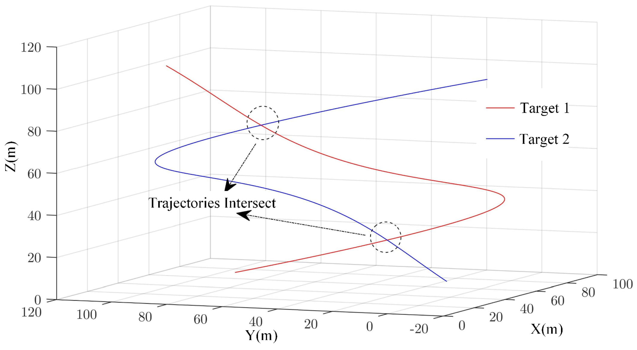
To evaluate the performance of the algorithm, we assume that two targets are relatively close and their trajectories intersect.
As shown in Figure 4, two targets’ trajectories are overlapped when they are close to the intersecting point. We set their trajectories as follows:
Target 1:
x ( k ) = 50 × sin ( 2 π k / 102 ) + 50 y ( k ) = 0.04 × ( k 50 ) 2 z ( k ) = k
Target 2:
x ( k ) = 50 × sin ( 2 π k / 102 ) + 50 y ( k ) = 0.04 × ( k 50 ) 2 + 100 z ( k ) = k
where k is a parameter of the trajectory. The sampling interval is 1 s. We stipulate that when the distance between two targets is less than 100 m, the targets enter a dense area. In addition, the distance threshold χ between two targets is set to 3. One system node and four observation nodes are deployed in the three-dimensional space, which are designated as the monitoring system. The vertexes’ coordinates ( x , y , z ) of the dense area are ( 1 , 1 , 1 ) , ( 100 , 100 , 100 ) , ( 1 , 100 , 1 ) , ( 100 , 1 , 1 ) respectively.
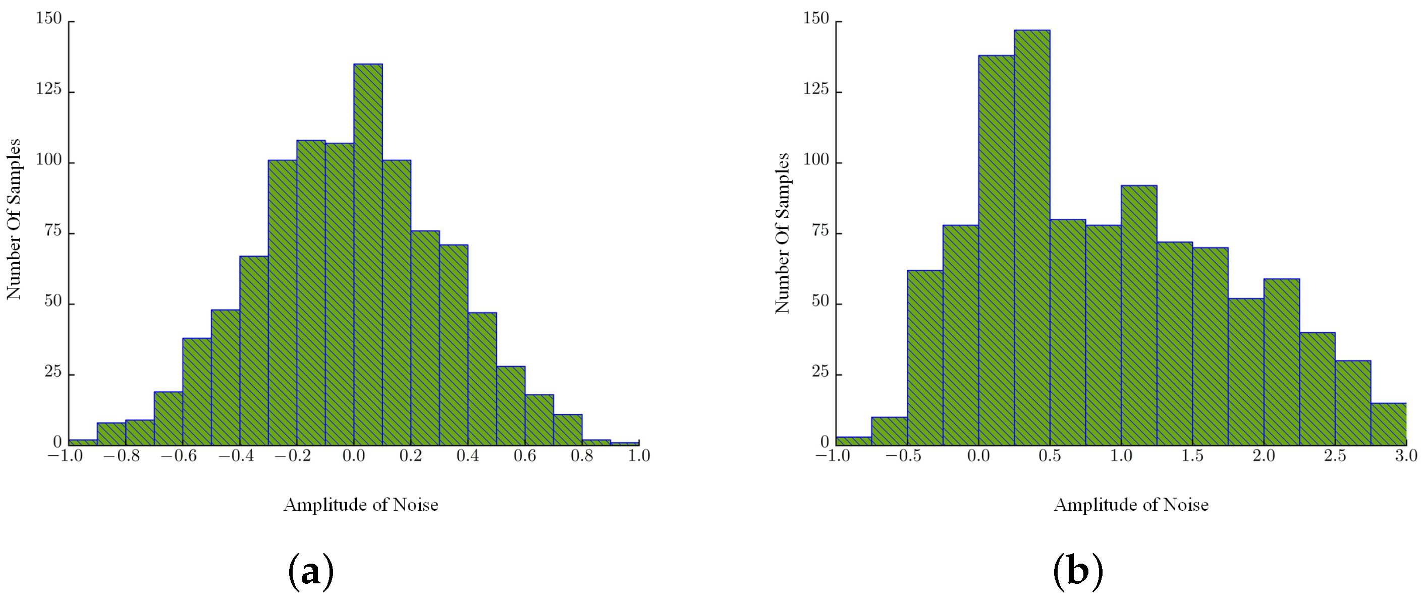
To verify the reliability and tracking accuracy of the proposed underwater target tracking algorithm for a non-Gaussian and nonlinear system, false alarms and noise interference are added to the observation of each node. Considering the complexity of underwater environment, the observation noise is modeled as a complex Gaussian mixture noise (GMN) model:
GMN = GN + 0.5 × randn + 2 × randn + 3 × randn + 6 × randn
( 0.5 × randn ) , ( 2 × randn ) , ( 3 × randn ) , ( 6 × randn ) represent Gaussian noises with different variances, which can be viewed as the random variances of the Gaussian mixture noise.
Figure 5 shows the noise distribution in the simulation with 1000 samples. Figure 5a,b illustrate the histograms of different noise amplitude’s counts under Gaussian noise and Gaussian mixture noise.
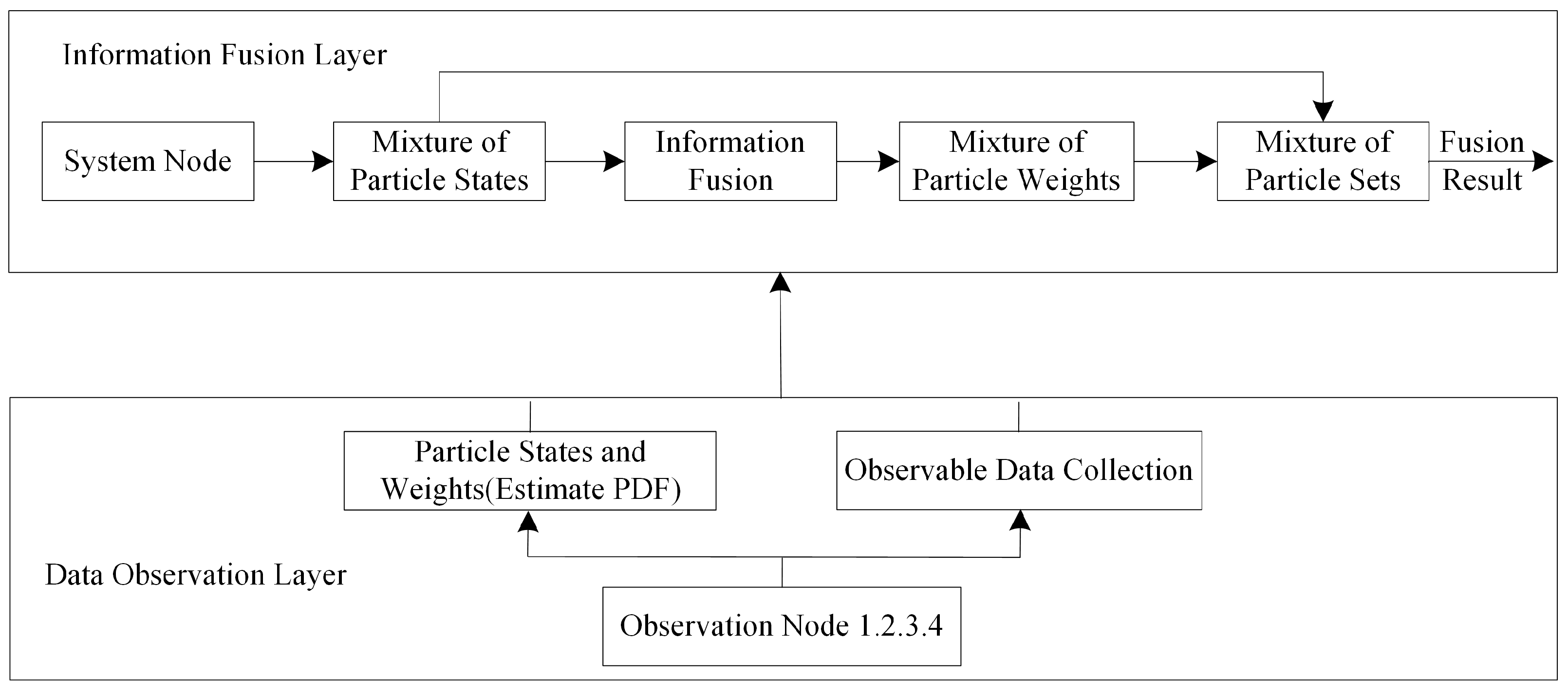
The accuracy of the posterior estimation for the target’s real state in the particle filter is positively correlated with the number of particles. However, the computation complexity of the algorithm also increases when the number of particles becomes larger. Considering this dilemma, we set the number of particles according to the task complexity of different layers. In the data observation layer, the demand for particle numbers is not high for the measurement and processing of distance information. However, the information fusion layer’s particle filter involves the global state estimation, so sufficient particles are required to ensure accurate estimation. Therefore, we set particle numbers of the data observation layer and the information fusion layer to 1000 and 10,000 respectively.

4.2. Comparison and Analysis

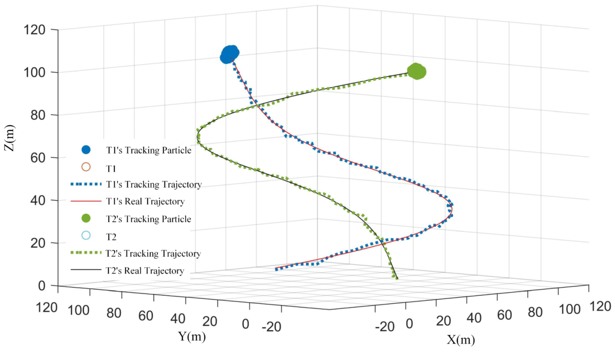
According to the above setting, under the interference of Gaussian mixture noises, the tracking results of the proposed algorithm in three-dimensional space are shown in Figure 6. The tracking accuracy keeps relatively high with minor bias when targets are close to each other but not intersecting in the dense area. Even when the targets intersect in a short time interval, the states and trajectories of the targets can still be accurately obtained. The tracking accuracy is relatively high in the whole process of simulation without significant degradation in the given monitoring area, which proves the effectiveness of the proposed algorithm.
In order to verify the advantages of TLPF-DPF positioning algorithm, we compare it with the particle filter algorithm based on distributed fusion (PF-DF) [30] and the extended Kalman filter algorithm based on distributed fusion (EKF-DF) [31] under the same model and scenario setting. For the filtering algorithms in [30,31]. We apply them to the distributed structure and use their classical state estimation methods to track underwater targets.
Table 1 and Table 2 list the average error ( e a v e ), maximum error( e m a x ) and minimum error( e m i n ) of different methods with Gaussian noise and Gaussian mixture noise. The standard deviation of the error ( e s t d ) is also listed in Table 2. Figure 7a,b illustrate the positioning errors under Gaussian noise. 
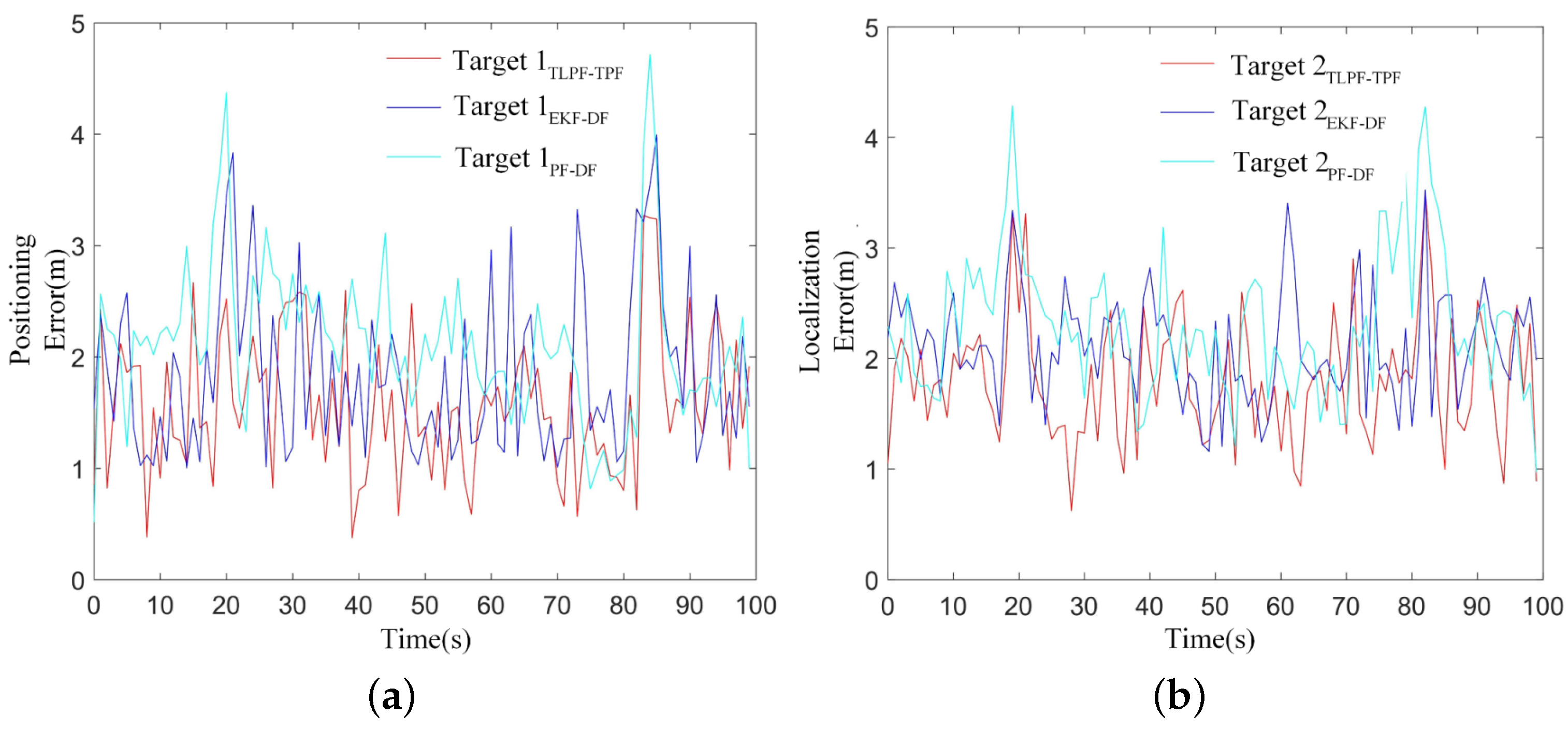
Figure 8a,b illustrate the positioning errors under Gaussian mixture noise.
From Table 1 and Table 2, we can conclude that the proposed algorithm achieves higher multi-target tracking accuracy in the presence of complex noises. Compared with PF-DF, its average positioning error is less by nearly 30%. Owing to the usage of the dynamic network resource allocation mechanism, the positioning accuracy of the three algorithms is relatively high and stable, which illustrates that the proposed dynamic allocation mechanism can support positioning algorithms for accurate and efficient observation under Gaussian noise.
Under Gaussian noises, it can be seen from Figure 7a,b that the positioning error increases when the two targets enter the intersecting region when t = 20 s and t = 83 s. However, the proposed algorithm achieves higher positioning accuracy in the intersecting region through the whole tracking process.
According to Figure 8a,b, when targets are close to each other under Gaussian mixture noise, the proposed method also achieves higher tracking accuracy compared with other methods. Even in the intersecting region, the proposed method can still ensure stable tracking performance while other methods degrade significantly.
Since the initial states plays a vital role in the traditional particle filter algorithm, we tend to evaluate the robustness of the proposed algorithm under different initial states. We change the initial state by adding a Gaussian noise κ × randn to it, where randn is a standard normal distribution and κ is a parameter of standard deviation. The results are shown in Table 3.
According to Table 3, we can draw the conclusion that different initial states of nodes do not lead to an significant performance degradation, which proves the robustness of the proposed algorithm.
Next, we change the number of particles in the information fusion layer to illustrate its affect on the proposed algorithm. The details are shown in Table 4, where N is the number of particles.
As shown in Table 4, the average error e a v e decreases with the number of particles increases, which matches the characteristics of particle filter algorithm.
We also change the velocity of target 1 by adjusting a parameter v. The trajectory of target 1 is:
x ( k ) = v × sin ( 2 π k / 102 ) + 50 y ( k ) = 0.04 × ( k 50 ) 2 z ( k ) = k
As shown in Table 5, the change in target 1 ‘s velocity has little impact on the average error, which illustrates the good stability of the proposed algorithm.
Besides, the uncertainty of the target’s trajectory may also have negative effects on the target tracking algorithm. To evaluate our proposed algorithm, we add a Gaussian noise on the y-axis of target 1’s trajectory. The trajectory of target 1 becomes:
x ( k ) = 50 × sin ( 2 π k / 102 ) + 50 y ( k ) = 0.04 × ( k 50 ) 2 + λ × r a n d n z ( k ) = k
where λ is the standard deviation of the Gaussian noise. The results are shown in Table 6.
As shown in Table 6, the influence of different λ on the average error e a v e is minor, which illustrates the robustness of our proposed algorithm.
We also evaluate our proposed algorithm with different kinds of non-Gaussian noises. Concretely, three different types of non-Gaussian noises are designed:
G 1 = U ( 0 , 20 )
G 2 = Laplace ( 0 , 20 )
G 3 = Exp ( 30 )
where G 1 is a uniform distribution, G 2 is a Laplace distribution and G 3 is an exponential distribution. The results are shown in Table 7.
As shown in Table 7, e a v e keeps within an acceptable range, which illustrates that the proposed algorithm can effectively cope with different non-Gaussian noises.
Moreover, we have tested our proposed algorithm on a Raspberry Pi (RPi) with a 1.4-GHz 64-bit quad-core processor, which is an applicable hardware setup for underwater monitoring network. Since the computation cost mainly depends on the particle filter algorithm for information fusion, we evaluate the average running time of the proposed algorithm in the information fusion layer with different numbers of particles. The details are shown in Table 8.
In practical, N = 5000 is sufficient for accurate target tracking, the running time when N = 5000 can be neglected compared with the expensive data communication in the underwater environment. Thus, the time complexity of the proposed algorithm is acceptable for real-time applications.
To sum up, the proposed multi-target tracking algorithm can deal with complex environmental noises and the scenario when targets’ trajectories intersect, which achieves better performance compared with other tracking methods in terms of positioning accuracy and stability.

5. Conclusions and Future Work

In this paper, we study the multi-targets’ tracking process in a dense underwater area. In order to improve the tracking performance under the impact of environmental interference, a position estimation model based on geometric constraints and a dynamic allocation mechanism of network resources based on prior position estimation are proposed to reduce the difficulty of obtaining observations and accurate initial states. On this basis, we propose an underwater multi-target tracking algorithm based on TLPF-DPF to deal with the complex noises and observation mismatching problem when targets’ trajectories intersect. Finally, the simulation is carried out with multiple targets in the three-dimensional dense underwater area. The results show that the proposed method improves the accuracy and robustness of multi-target tracking when targets’ trajectories intersect.
In future work, we intend to establish a model that can Further reduce computational complexity to ensure the scalability of the algorithm. Additionally, we aim to consider the impact of underwater communication delay and packet loss to make the algorithm more robust to extreme underwater environments.

Author Contributions

Conceptualization, K.K.; methodology, K.K.; software, B.L.; validation, B.L.; formal analysis, L.D.; investigation, K.K.; resources, L.D.; data curation, B.L.; writing—original draft preparation, K.K.; writing—review and editing, L.D.; visualization, B.L.; supervision, L.S.; project administration, L.S. All authors have read and agreed to the published version of the manuscript.

Funding

This research was funded by the Key Laboratory Fund of National Defense Science and Technology under Grant 2022JCJQLB03308, the Joint Fund of Equipment Pre-Research and Ministry of Education under Grant 8091B022235, the National Natural Science Foundation of China under Grant 62203299, and the Oceanic Interdisciplinary Program of Shanghai Jiao Tong University under Grants SL2022MS010 and SL2022MS008.

Institutional Review Board Statement

Not applicable.

Informed Consent Statement

Not applicable.

Data Availability Statement

Not applicable.

Conflicts of Interest

The authors declare no conflict of interest.

References

  1. Cui, S.; Wang, Y.; Wang, S.; Wang, R.; Wang, W.; Tan, M. Real-time perception and positioning for creature picking of an underwater vehicle. IEEE Trans. Veh. Technol. 2020, 69, 3783–3792. [Google Scholar] [CrossRef]
  2. Qi, K.; Qu, G.; Xue, S.; Xu, T.; Su, X.; Liu, Y.; Wan, J. Analytical optimization on GNSS buoy array for underwater positioning. Acta Oceanol. Sin. 2019, 38, 137–143. [Google Scholar] [CrossRef]
  3. Leonard, M.R.; Zoubir, A.M. Multi-target tracking in distributed sensor networks using particle PHD filters. Signal Process. 2019, 159, 130–146. [Google Scholar] [CrossRef]
  4. Gao, L.; Battistelli, G.; Chisci, L.G. Event-triggered distributed multitarget tracking. IEEE Trans. Signal Inf. Process. Netw. 2019, 5, 570–584. [Google Scholar] [CrossRef]
  5. Zhang, J.; Hu, T.; Shao, X.; Xiao, M.; Rong, Y.; Xiao, Z. Multi-Target Tracking Using Windowed Fourier Single-Pixel Imaging. Sensors 2021, 21, 7934. [Google Scholar] [CrossRef] [PubMed]
  6. He, X.Y.; Wang, Y.; Yang, S.Q. Gaussian Mixture CBMeMBer Filter for Multi-Target Tracking with Non-Gaussian Noise. IAENG Int. J. Appl. Math. 2022, 52, 1–8. [Google Scholar]
  7. Zhang, W.Y.; Yang, F.; Liang, Y. Robust multi-target tracking under mismatches in both dynamic and measurement models. Aerosp. Sci. Technol. 2019, 86, 748–761. [Google Scholar] [CrossRef]
  8. Wang, Z.Y.; Zhou, W.D. Design and Implementation of Robust Particle Filter Algorithms under Student-t Measurement Distribution. J. Electron. Inf. Technol. 2019, 41, 12. [Google Scholar]
  9. Jahan, K.; Rao, S.K. Implementation of underwater target tracking techniques for Gaussian and non-Gaussian environments. Comput. Electr. Eng. 2020, 87, 106783. [Google Scholar] [CrossRef]
  10. Zhang, T.D.; Wan, L.; Wang, B.; Zeng, W.J. Underwater Object Tracking Based on Improved Particle Filter. J. Shanghai Jiaotong Univ. 2012, 46, 943–948. [Google Scholar]
  11. Yardim, C.; Michalopoulou, Z.; Gerstoft, P. An overview of sequential Bayesian filtering in ocean acoustics. IEEE J. Ocean. Eng. 2011, 36, 71–89. [Google Scholar] [CrossRef]
  12. Zhang, Y.; Gao, L.J. Target tracking with underwater sensor networks based on Grubbs criterion and improved particle filter algorithm. J. Electron. Inf. Technol. 2019, 41, 2294–2301. [Google Scholar]
  13. Singer, R.; Sea, R. New results in optimizing surveillance system tracking and data correlation performance in dense multitarget environments. IEEE Trans. Autom. Control 1973, 18, 571–582. [Google Scholar] [CrossRef]
  14. Wang, Y.J.; Li, Y.; Ju, D.H.; Huang, H.N. A Multi-target Passive Tracking Algorithm Based on Unmanned Underwater Vehicle. J. Electron. Inf. Technol. 2020, 42, 2013–2020. [Google Scholar]
  15. Jing, D.X.; Han, J.; W, G.Y.; Wang, X.D.; Wu, J.Y.; Chen, G.H. Dense multiple-target tracking based on dual frequency identification sonar (DIDSON). In Proceedings of the OCEANS 2016—Shanghai, Shanghai, China, 19–23 September 2016. [Google Scholar]
  16. Y, F.; Li, C.; Wang, H.B.; Yang, F. Automatic underwater acoustic target tracking by using image processing methods with jamming targets. In Proceedings of the 2021 China Automation Congress (CAC), Beijing, China, 22–24 October 2021. [Google Scholar]
  17. Djenouri, D.; Bagaa, M. Energy-aware constrained relay node deployment for sustainable wireless sensor networks. IEEE Trans. Sustain. Comput. 2017, 2, 30–42. [Google Scholar] [CrossRef]
  18. Jouhari, M.; Ibrahimi, K.; Tembine, H.; Ben-Othman, J. Underwater wireless sensor networks: A survey on enabling technologies, localization protocols, and internet of underwater things. IEEE Access 2019, 7, 96879–96899. [Google Scholar] [CrossRef]
  19. Ranjha, A.; Kaddoum, G.; Rahim, M.; Dev, K. URLLC in UAV-enabled multicasting systems: A dual time and energy minimization problem using UAV speed, altitude and beamwidth. Comput. Commun. 2022, 187, 125–133. [Google Scholar] [CrossRef]
  20. Narsani, H.K.; Ranjha, A.; Dev, K.; Memon, F.H.; Qureshi, M.F. Leveraging UAV-assisted communications to improve secrecy for URLLC in 6G systems. Digit. Commun. Netw. 2022. [Google Scholar] [CrossRef]
  21. Asif, M.; Ihsan, A.; Khan, W.H.; Ranjha, A.; Zhang, S.; Wu, S.X.; Wu, S.X. Energy-Efficient Backscatter-Assisted Coded Cooperative-NOMA for B5G Wireless Communications. IEEE Trans. Green Commun. Netw. 2022, 7, 70–83. [Google Scholar] [CrossRef]
  22. Meyer, F.; Braca, P.; Hlawatsch, F.; Micheli, M.; LePage, K.D. Scalable adaptive multitarget tracking using multiple sensors. In Proceedings of the 2016 IEEE Globecom Workshops (GC Wkshps), Washington, DC, USA, 4–8 December 2016. [Google Scholar]
  23. Sun, D.J.; Zheng, C.E.; Cui, H.Y.; Zhang, J.C.; Han, Y.F. Developing status and some cutting-edge issues of underwater sensor network localization technology. Sci. China Inf. Sci. 2018, 48, 1121–1136. [Google Scholar] [CrossRef]
  24. Diamant, R.; Lampe, L. Low probability of detection for underwater acoustic communication: A review. IEEE Access 2018, 6, 19099–19112. [Google Scholar] [CrossRef]
  25. Yuan, Y.Z.; Li, Y.F.; Liu, Z.X.; Chan, K.Y.; Zhu, S.Y.; Guan, X.P. A three dimensional tracking scheme for underwater non-cooperative objects in mixed LOS and NLOS environment. Peer-to-Peer Netw. Appl. 2019, 12, 1369–1384. [Google Scholar] [CrossRef]
  26. Savic, V.; Zazo, S. Cooperative localization in mobile networks using nonparametric variants of belief propagation. Ad Hoc Netw. 2013, 11, 138–150. [Google Scholar] [CrossRef]
  27. Wang, S. Distributionally Robust State Estimation for Nonlinear Systems. IEEE Trans. Signal Process. 2022, 70, 4408–4423. [Google Scholar] [CrossRef]
  28. Gong, Y.; Yang, H.; Hu, W.; Yu, W. An efficient particle filter based distributed track-before-detect algorithm for weak targets. In Proceedings of the IET International Radar Conference, Guilin, China, 20–22 April 2009. [Google Scholar]
  29. Gustafsson, F. Particle filter theory and practice with positioning applications. IEEE Aerosp. Electron. Syst. Mag. 2010, 25, 53–82. [Google Scholar] [CrossRef]
  30. Lim, J.; Shin, M.; Hwang, W. Variants of extended Kalman filtering approaches for Bayesian tracking. Int. J. Robust Nonlinear Control 2017, 27, 319–346. [Google Scholar] [CrossRef]
  31. Lu, F.; Gao, T.Y.; Huang, J.Q.; Qiu, X.J. A novel distributed extended Kalman filter for aircraft engine gas-path health estimation with sensor fusion uncertainty. Aerosp. Sci. Technol. 2019, 84, 90–106. [Google Scholar] [CrossRef]
Figure 1. Diagram of network resource dynamic allocation mechanism.
Jmse 11 00858 g001
Figure 2. Distance observation model.
Jmse 11 00858 g002
Figure 3. Processing procedure of multi-target tracking algorithm.
Jmse 11 00858 g003
Figure 4. Trajectories of targets in the dense area.
Jmse 11 00858 g004
Figure 5. Amplitude distribution histogram of compound noise. −1 (a) Histogram of Gaussian noise distribution. (b) Histogram of Gaussian mixture noise distribution.
Jmse 11 00858 g005
Figure 6. Trajectories of targets’ tracking in 3D space.
Jmse 11 00858 g006
Figure 7. Targets’ Tracking Error Under Gaussian Noise. (a) Target 1’s Positioning Error under Gaussian Noise. (b) Target 2’s Positioning Error under Gaussian Noise.
Jmse 11 00858 g007
Figure 8. Targets’ Tracking Error Under Gaussian Mixture Noise. (a) Target 1’s Positioning Error under Gaussian Mixture Noise. (b) Target 2’s Positioning Error under Gaussian Mixture Noise.
Jmse 11 00858 g008
Table 1. Comparison of positioning errors with Gaussian noise.
TargetMethod e max e min e ave
Target 1TLPF-DPF3.1670.4761.583
Target 1PF-PF3.5330.9561.767
Target 1EKF-PF3.6570.5141.990
Target 2TLPF-DPF3.5670.6241.794
Target 2PF-PF3.5231.1612.016
Target 2EKF-PF4.2840.9702.205
Table 2. Comparison of positioning errors with Gaussian mixture noise.
TargetMethod e max e min e ave e std
Target 1TLPF-DPF3.5670.4761.7830.947
Target 1PF-PF4.7221.0652.4741.065
Target 1EKF-PF6.6570.7143.5411.579
Target 2TLPF-DPF3.4970.6241.8140.802
Target 2PF-PF4.6211.3482.5170.905
Target 2EKF-PF6.2841.6153.7921.339
Table 3. Comparison of positioning errors with different initial states.
Target κ e max e min e ave
Target 116.2490.5031.863
Target 128.1110.8102.072
Target 139.9691.1752.381
Target 216.7020.4151.848
Target 227.4480.9102.196
Target 239.1661.2832.290
Table 4. Comparison of positioning errors with different number of particles.
TargetN e max e min e ave
Target 120006.3872.1054.143
Target 150004.7551.6492.202
Target 110,0003.3660.3571.733
Target 220006.7942.7773.500
Target 250004.3081.2162.255
Target 210,0003.4360.3811.825
Table 5. Comparison of positioning errors with different velocity of target 1.
Targetv e max e min e ave
Target 120003.6030.2141.771
Target 150003.5960.1871.719
Target 1100003.6820.5581.814
Table 6. Comparison of positioning errors with different Gaussian noise of target 1’s trajectory.
Target λ e m a x e m i n e a v e
Target 10.13.6990.2101.764
Target 10.53.6640.2231.775
Target 113.7120.2021.781
Table 7. Comparison of positioning errors with non-Gaussian noises.
TargetNoise e max e min e ave
Target 1 G 1 3.0970.4451.313
Target 1 G 2 2.6410.1831.485
Target 1 G 3 3.0370.1391.411
Table 8. Running time of the proposed algorithm.
N5001000500010,000
Time (s)0.0190.0790.6471.623
Disclaimer/Publisher’s Note: The statements, opinions and data contained in all publications are solely those of the individual author(s) and contributor(s) and not of MDPI and/or the editor(s). MDPI and/or the editor(s) disclaim responsibility for any injury to people or property resulting from any ideas, methods, instructions or products referred to in the content.

