Time Variation Trend of Wave Power Density in the South China Sea

Abstract

Based on the third-generation wave model WAVEWATCH-III (WW3), this paper analyzes the changing trend of wave power density (WPD) in the South China Sea, which can provide necessary references for the development and utilization of wave energy resources in the future. In this study, multi-platform cross-calibrated (CCMP) wind data was used to drive WW3 to calculate the WPD of the South China Sea. The Mann-Kendall (MK) algorithm can be used to determine the mutation of WPD, and the accuracy of the CCMP wind was verified. Next, the time distribution of WPD is analyzed for the whole sea area and dominant sea area of the South China Sea, and on this basis, the dominant sea area for the development of wave energy resources in the South China Sea was studied. The results are as follows: (1) Extreme weather has a significant impact on the change of WPD in the South China Sea, and this change is likely due to the effect of extreme weather on sea temperature. (2) Dongsha Islands has the highest annual WPD value and has the greatest impact on the overall trend change of the South China Sea. (3) Integrated wave energy exploitability and safety and technology perspectives, the waters around Taiwan Strait are more suitable as the primary site for energy conversion.

1. Introduction

In today’s world, coal and other conventional energy are increasingly scarce, and countries around the world have begun to promote the application of clean energy to deal with the energy crisis. Wave energy gets the favor of all countries due to no pollution, renewable, large reserves, and so on. The South China Sea is a connecting hub connecting the western Pacific Ocean and the North Indian Ocean, which is rich in Marine resources and has a prominent strategic location. Therefore, it is necessary to study the WPD distribution in the South China Sea to facilitate the subsequent development.

In the past, many scholars have made a lot of contributions to wave power density analysis, and wave power density analysis can be divided into observation data stage, satellite data stage, and numerical simulation stage according to the data source. In the observation data stage, people use ocean ship reports and buoy data to calculate the size of the global coastal wave power density. Thorpe [1] analyzed the WPD around the UK through observation data. Lenee-Bluhm et al. [2] used NDBC (National Data Buoy Center) and CDIP (Coastal Data Information Program) data to analyze the wave energy resources in the Pacific Ocean in the northwest of the United States. In the satellite data stage, satellite observations are applied to wave energy research. For example, Barstow et al. [3] used the effective wave height retrieved from TOPEX/Poseidon satellite altitude and data to calculate the WPD of hundreds of stations near the global coast. Wan [4] also used the AVISO data from 2009 to 2013 to analyze the wave energy characteristics in Chinese waters. In the numerical simulation stage, many wave models were widely applied for evaluating wave energy, such as WAM (Wave Action Model), WW3(WAVEWATCH-III), and SWAN (Simulation Waves Nearshore). Kompor et al. [5] discussed the wave energy resources in Thailand under three monsoon conditions with the help of the SWAN model. Li Chongyin et al. [6] analyzed the spatiotemporal characteristics of Indian Ocean waves based on the WW3 model using 45-year ERA-40 wind data. Goncalves [7] analyzed the wave energy status of the west coast of France by using the combination of WW3 and SWAN models. Liberti et al. [8] used the WAM model to analyze the wave energy resource pattern of the Mediterranean Sea in the past 10 years.

For the South China Sea studied in this paper, there have been previous studies. For example, Zheng Chongwei et al. [9] simulated and evaluated the wind energy and wave energy in the East China Sea and South China Sea with 22 years of CCMP wind field data and WW3 model and analyzed the evaluation results. Zhifeng Wang et al. [10] evaluated the long-term wind and wave energy resources of the South China Sea by combining the Weather Research and Prediction Model (WRF) and WW3 model and determined the main wave direction and total energy amount of the South China Sea.

The spatial distribution of WPD has been extensively studied by scholars. While the research on the long-term trend and stability of WPD is important in practice, there are few relevant studies. Especially for the South China Sea studied in this paper, there are even fewer relevant studies on the long-term variation trend of WPD. The South China Sea is one of the two key bodies of water of China’s “Maritime Silk Road” and plays a pivotal role in the strategy of maritime power. Therefore, it is necessary to study the long-term trend of WPD in the South China Sea. On the basis of previous studies, this paper studied the time variation trend of WPD in the South China Sea and further studies the WPD variation trend of the dominant sea areas in the South China Sea. Based on this, it determines which of these dominant sea areas are suitable for further development of wave energy and how extreme weather affect the variation of WPD in the South China Sea. It is hoped to provide a necessary reference for the development and utilization of wave energy resources in the future and the zoning of the navigation area.

2. Methods

The purpose of this study is to determine the change in wave power density in the South China Sea from 1990 to 2017. In this paper, 28-year wave data was calculated by WW3, and the MK algorithm was used to study the change in wave power density.

2.1. WW3 Model

2.1.1. Numerical Simulation Method of Wave Energy

The parameters related to WW3 were set as follows: the sea area calculated by WW3 was set as 104° E~125° E and 4° N~27° N, which contains the main part of the South China Sea and surrounding waters; the topographic map of the South China Sea was shown in Figure 1. The computing time range was from 1 January 1990, to 31 December 2017. The spatial resolution of the WW3 model was 0.25° × 0.25°, and the time step of calculation was 300 s. The results of WW3 calculation were output every 6 h.

2.1.2. Wave Power Density Calculation Method

In order to calculate the 28-year variation trend of WPD in the South China Sea, it is necessary to determine the formula for calculating the WPD. Two main parameters, wave height and wave period are needed to calculate this feature. According to the selection of Behrens et al. [11,12], the wave power density calculation method are as follows:

In shallow water (d/λ < 1/20), the calculation method is as follows:

$$P_w=\frac{\rho g}{16}{H}_S^2\sqrt{gd}$$

(1)

In medium water depth (1/20 ≤ d/λ < 1/2), calculation method is as follows:

$$P_w=\overline{E}(\frac{g{T}_e}{2\pi }\tanh kd)[\frac{1}{2}(1+\frac{2kd}{\sinh 2kd})]$$

(2)

In deep water (d/λ ≥ 1/2), the calculation method is as follows:

$$P_w=\frac{\rho g^2{H}_s^2{T}_0}{64\pi }$$

(3)

where $H_S$ is the wave height, $T_o$ is the energy density, $P_w$ denotes the wave power density, $\lambda$ is wave length, and $d$ is the water depth

According to the research of Luca and Rusu et al. [13], the density of seawater is about 1015 $\mathrm{k}\mathrm{g}/{\mathrm{m}}^3$, which is 9.80 $\mathrm{m}/{\mathrm{s}}^2$ for gravitational acceleration and 3.14 for PI. Therefore, Formula (3) can be further simplified to formula (4):

$$P_w=0.484H_s^2{T}_0$$

(4)

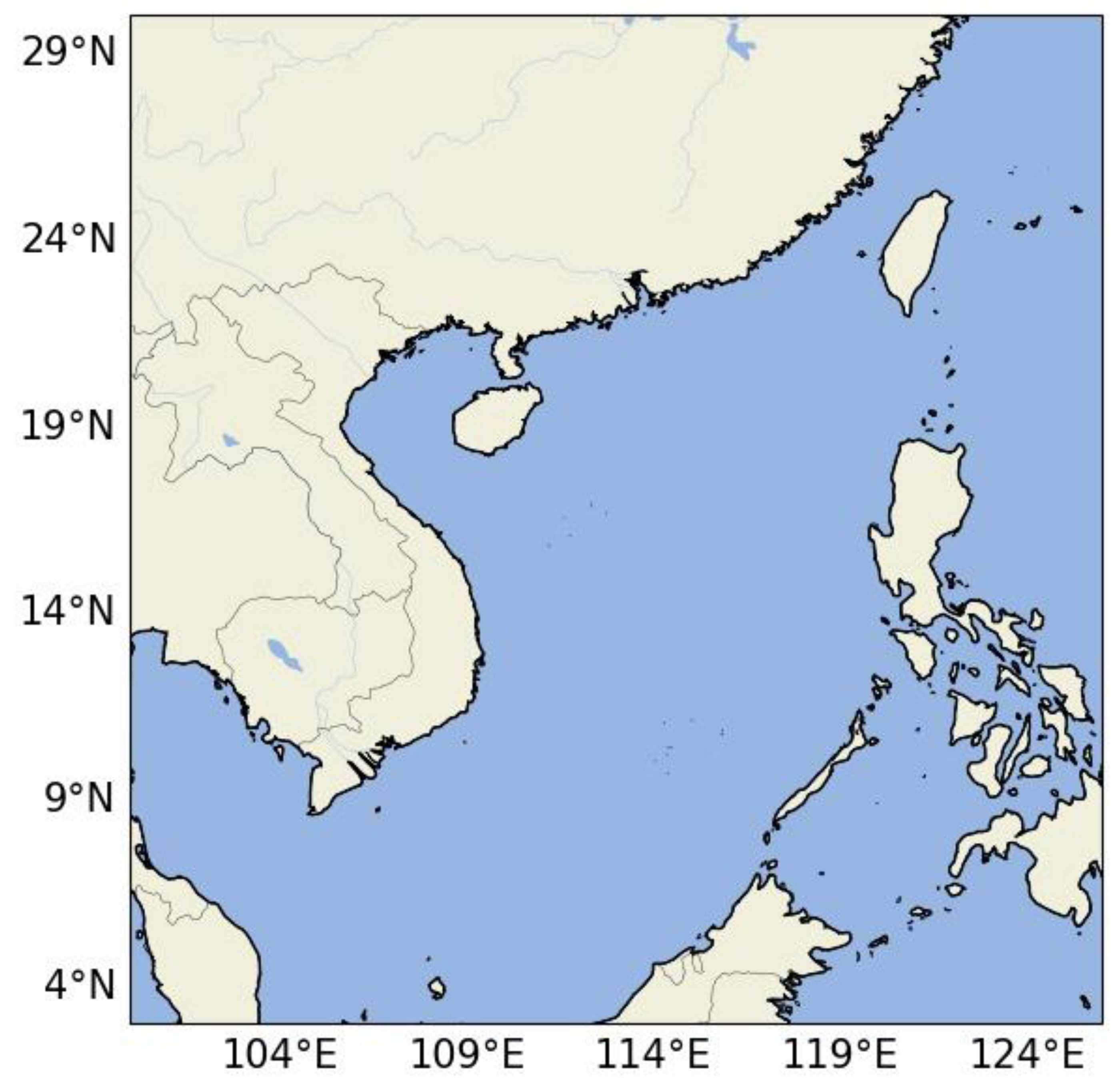
2.1.3. Wind Field Data and Topographic Data

For running the WW3 wave model, the ETOPO5 (5-Minute Gridded Global Relief Data Collection) topographic dataset, CCMP wind data, was used. The CCMP wind data was used as the driving data of the WW3 wave model, which was widely used in scientific research due to its accuracy. The spatial range is 180° W–180° E, 90° S–90° N, with a spatial resolution of 0.25 × 0.25 and the time resolution of 6 h. Besides that, ETOPO5 high-resolution topographic dataset is derived from U.S National Geophysical Data Center, and the spatial resolution is 5′ × 5′. The dataset has bathymetric data, digitized land, and detailed bathymetric and topographic information for the study area.

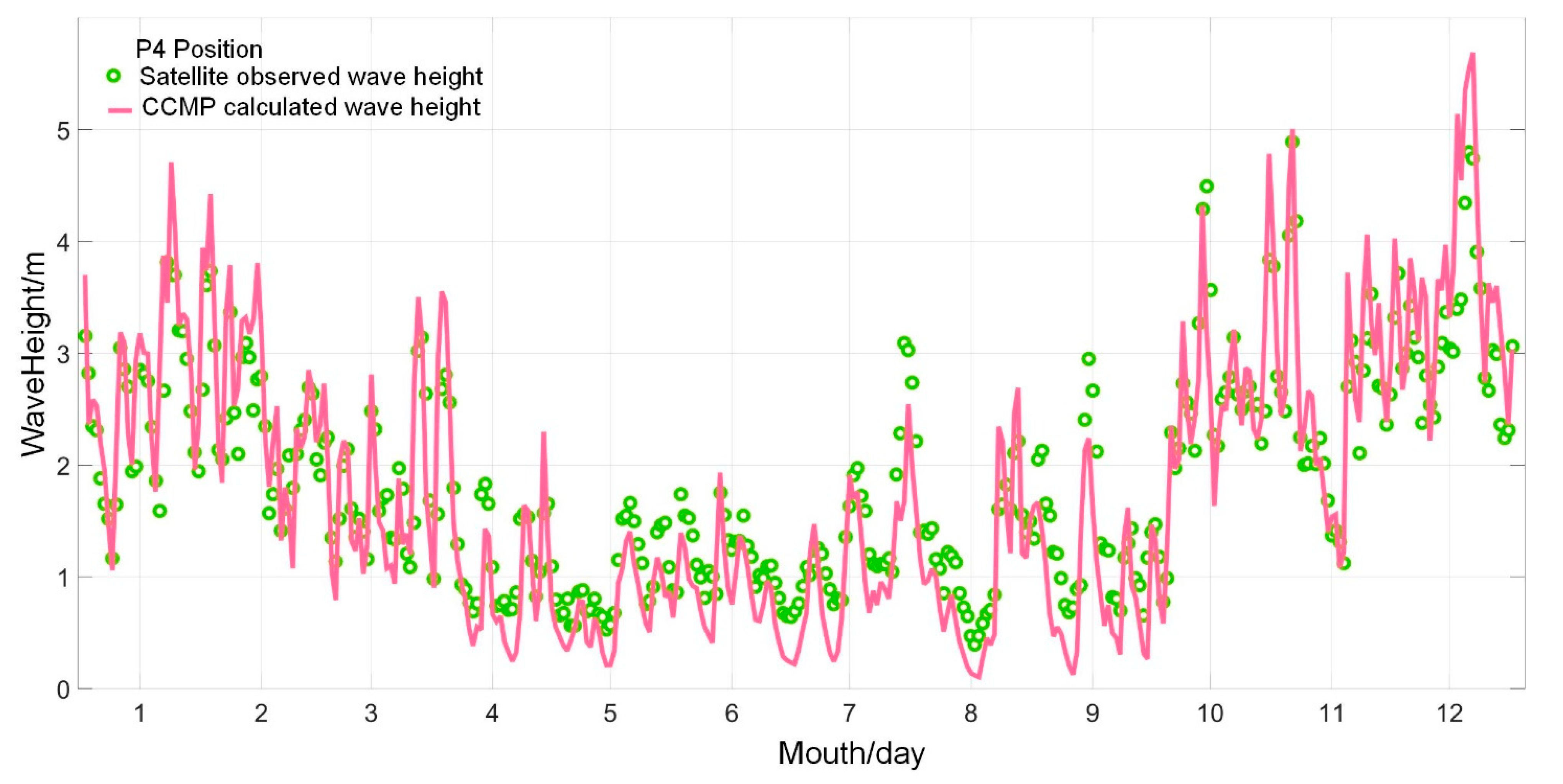
2.1.4. Observed Wave Data

The satellite altimeter data provided by Jason-2 was used for the accuracy test of WW3, and the time range is 1 January 2017, to 31 December 2017. The Jason2 satellite has a repetition period of about 10 days, an orbital altitude of 1336 km, and an orbital inclination of 66°. In addition, Jason2 carries a Poseidon-3 altimeter, a radiometer, and three positioning systems to complete high-precision altimetry tasks. The Poseidon-3 altimeter can transmit pulses of two frequencies (13.6 GHZ and 5.3 GHZ) with a pulse duration of 105 ms, a power of 7 W, a 1.2 m antenna diameter, and a measurement accuracy of approximately 2.5 cm.

Jason-2 data can not only provide the all-weather and full range of wave height data but also ensure the reliability of data under long time series. Therefore, it is increasingly favored by researchers in the numerical prediction of ocean waves and plays an important role in the testing of effective wave height.

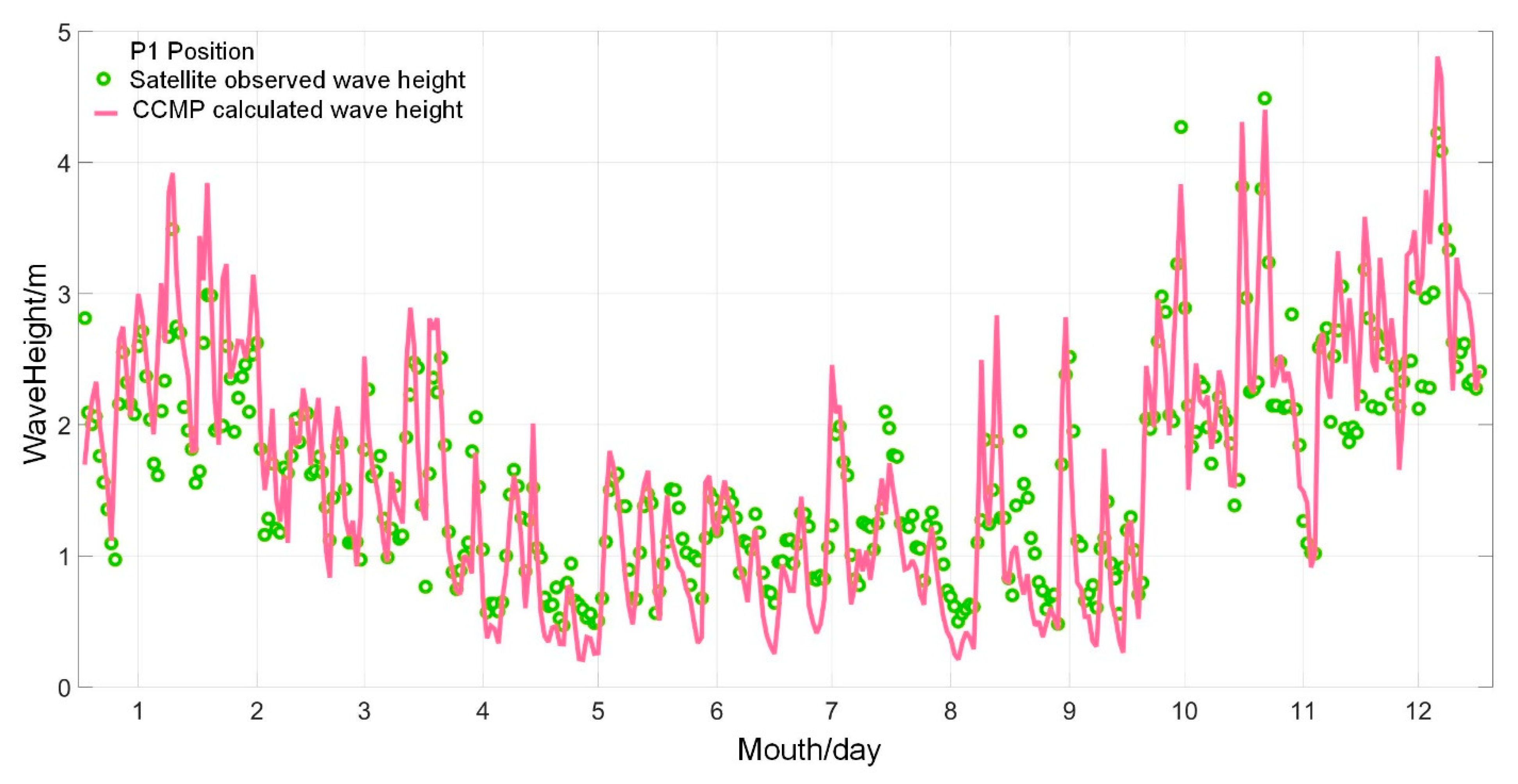
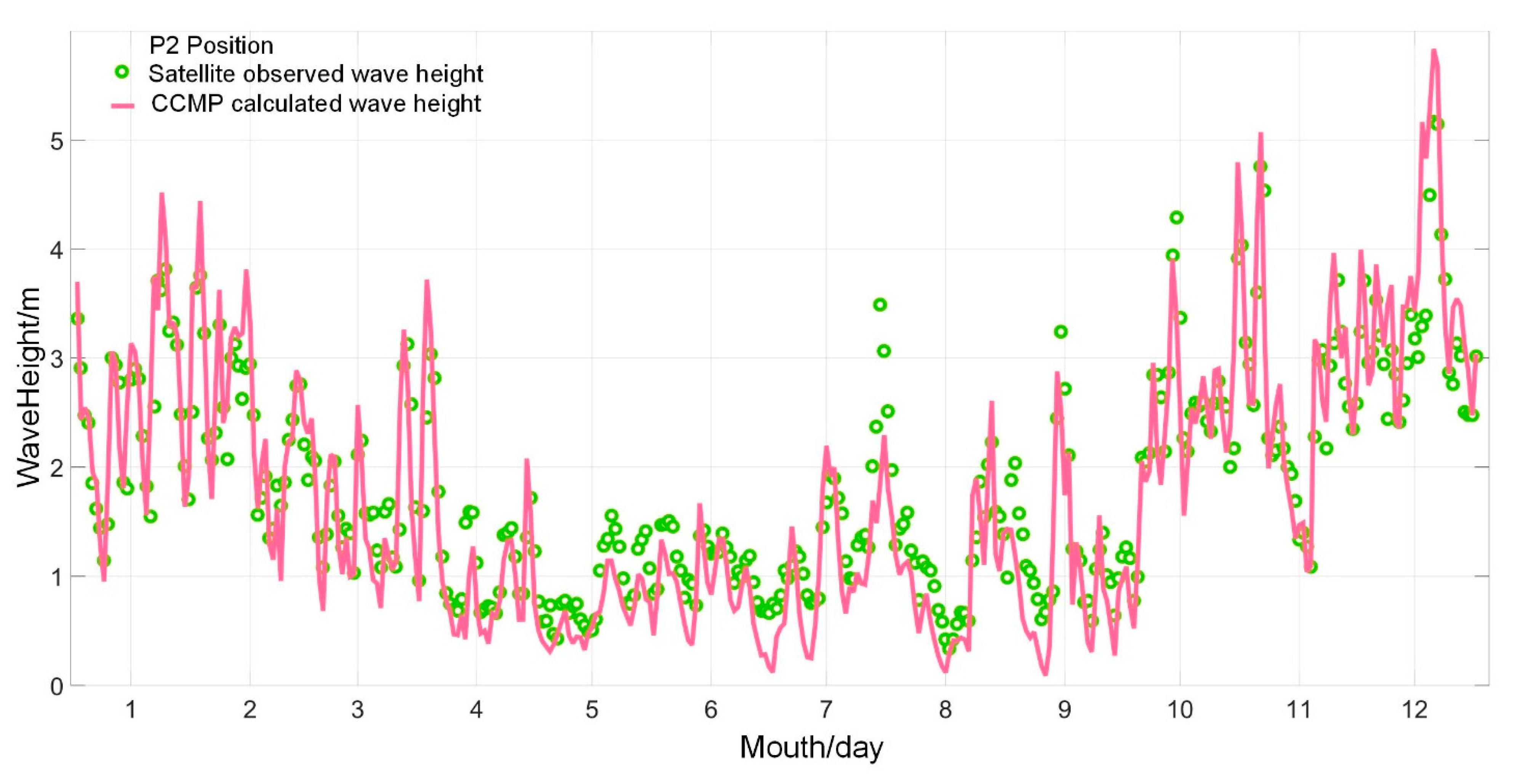
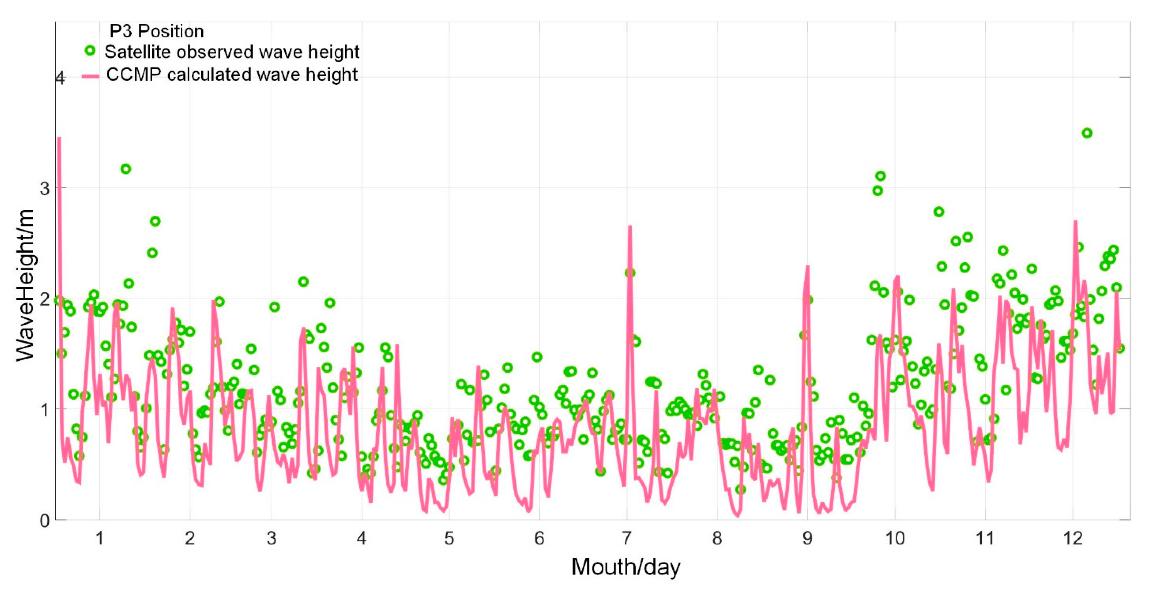
2.1.5. Validation of the WW3 Data

In order to determine the suitability of the CCMP wind field to simulate the wave height of the South China Sea, the calculation results of WW3 were compared with the satellite altimeter data. Four points (P1–P4) are selected in the calculation sea area to compare the calculated results of WW3 with the observed values of the altimeter, so as to determine whether the calculated results of WW3 meet the accuracy requirements. The specific position of P1 is (20° N, 113° E), P2 is (18° N, 116° E), P3 is (20° N, 108° E), and P4 is (19° N, 117° E).

Next, the calculation results of WW3 at these four points are compared with the satellite altimeter observations, and the comparison results are plotted. Among them, Figure 2 shows the comparison results between the calculated values of WW3 at P1 and the observed values of the satellite altimeter, Figure 3 shows the comparison results between the calculated values of WW3 at P2 and the observed values of the satellite altimeter, Figure 4 shows the comparison results between the calculated values of WW3 at P3 and the observed values of the satellite altimeter, and Figure 5 was obtained by comparing the calculated results at P4 with the satellite altimeter observations.

Figure 2 shows that at P1, the calculation results of WW3 are close to the satellite observation data, and the overall difference is not large. Figure 3 shows that the calculated results of WW3 at P2 are also basically consistent with the satellite observation data. Figure 4 shows that although the overall trend of WW3 at P3 is similar to that of satellite observation data, the calculated value of WW3 is generally smaller than that of satellite observation data. Figure 5 shows that the variation trend of WW3 at P4 is relatively similar to that of satellite observation data, and the numerical difference is not large.

In addition, the statistics were used to determine the accuracy of WW3 calculation results. Test statistics include correlation coefficient (CC), mean deviation (MAE), and root mean square error (RMSE).

Table 1. Precision of the simulated WVHT (Significant Wave Height).

	CC	MAE	RMSE
P1(20° N,113° E)	91.6%	−0.033 m	0.788 m
P2(18° N,116° E)	93.7%	0.078 m	0.954 m
P3(20° N,108° E)	65.9%	0.371 m	0.596 m
P4(19° N,117° E)	93.4%	0.053 m	0.936 m
Mean value	86.3%	0.117 m	0.818 m

shows the value of the statistics, and the following formulas were used to calculate the statistics in this paper:

$$CC=\frac{{\displaystyle \sum _{i=1}^N(P_i-\overline{P})(O_i-\overline{O})}}{{[{\displaystyle \sum _{i=1}^N{(P_i-\overline{P})}^2{\displaystyle \sum _{i=1}^N{(O_i-\overline{O})}^2}}]}^{1/2}}$$

(5)

$$RMSE=\sqrt{\frac{1}{N}{\displaystyle \sum _{i=1}^N{(P_i-O_i)}^2}}$$

(6)

$$MAE=\frac{1}{N}({\displaystyle \sum _{i=1}^N\left|P-\overline{P}\right|})$$

(7)

where $O_i$ represents observed data, $P_i$ represents simulated data, $\overline{P}$ and $\overline{O}$ are the average value of observed data and simulated data, respectively, $N$ is the total samples.

As can be seen from Table 1, the trend simulation of WVHT is the best at P2, and the correlation between simulated data and altimeter value is the strongest, reaching 93.7%, while the average deviation at P1 is the smallest, only −0.033 m. It is worth noting that the root mean square error of WVHT at P3 is the smallest, but the correlation coefficient is not high, and the average deviation is large. In general, the simulation effect of the WVHT is better in P1 and P2 than in P3 and P4.

In addition, as the selected data is the daily average data for the whole year of 2017, including the extreme weather that may occur throughout the year, such as typhoons, cyclones, and storms, it is understandable that there are errors. Based on the above reasons, it is decided to use the CCMP wind field to simulate the wave height in the South China Sea, and the subsequent WPD test will be completed on this basis.

2.2. Mann-Kendall Algorithm

In order to determine whether the WPD value has an abrupt change in climate and the time of the abrupt change, the MK algorithm is used to make a judgment. MK algorithm is a climate diagnosis and prediction technology. From the perspective of statistics, it belongs to the non-distribution test, and its advantage is that it does not need samples to follow a certain distribution, nor is it affected by a few outliers. It is more suitable for type and order variables, and its calculation is relatively simple.

Three tests are commonly used to test for mutation: the sliding t-test, the piecewise linear regression, and the Mann-Kendall test. The time cost of sliding t-test is high because it needs to constantly divide sub-sequences in the case of large data sets. The piecewise linear regression method is complex to calculate and needs to substitute more parameters, so it has no advantage in the case of a large amount of data. The subsequent research of this paper is based on the data from 1990 to 2017, and the amount of data is large. At this time, it is more convenient to use the Mann-Kendall algorithm to calculate and more efficient to judge the trend mutation, so the Mann-Kendall algorithm was used as the test method.

The mathematical principle is that the rank sum sequence is constructed in a time continuous sequence X (hereinafter referred to as the continuous sequence), where the number of samples of the rank sum sequence is n, and the expression is as follows:

$$S_k={\displaystyle {\sum }_{i=1}^k{\displaystyle {\sum }_{j=1}^i{r}_{ij} }}{r}_{ij}=\left\{\begin{array}{cc}1& x_i>x_j,j=1,2,\dots ,i\\ 0& else\end{array}\right.$$

(8)

The rank-sum sequence $S_k$ is the sum of the comparison threshold values of the value at the time i and the value at time j of each sample in the samples. It is assumed that the sequential sequence X is independent and randomly distributed by defining a new statistic:

$$U{F}_k=\frac{S_k-E(S_k)}{\sqrt{Var(S_k)}}, k=1,2,\dots ,n$$

(9)

Specify that $U{F}_1=0$, $E(S_k)$ and $Var(S_k)$ are respectively the mean and variance of the rank sum sequence. If the sequential sequence $x_1,x_2,x_3\dots x_n$ is independent of each other and uniformly distributed continuously, it can be calculated by the following Equations (6) and (7):

$$E(S_k)=\frac{n(n+1)}{4}$$

(10)

$$Var(S_k)=\frac{n(n-1)(2n+5)}{72}$$

(11)

$U{F}_i$ is subject to the standard normal distribution. This statistic series is calculated according to the time series. Then construct the reverse sequence $x_n,x_{n-1},x_{n-2}\dots x_1$ of the time continuous sequence X, repeat the above process, and let:

$$U{B}_k=-U{F}_k, k=n,n-1,\dots ,1$$

(12)

In addition to determining the specific mutation time, its mathematical principle is simple, the code is convenient to execute, and the practicability and operability are strong, so it is a suitable and efficient mutation detection method. Assume that the significance level $\alpha$ is set at 0.05, and the judgment method is as follows: when the statistic $U{F}_k>0$, it is 95% sure that sample X has an upward trend, $U{F}_k<0$ is considered that sample X shows a downward trend. If $\left|U{F}_i\right|>U\raisebox{1ex}{$\alpha $}\!\left/ \!\raisebox{-1ex}{$2$}\right.$, there is a 95% probability that X has a significant increase or decrease trend; If $\left|U{F}_i\right|<U\raisebox{1ex}{$\alpha $}\!\left/ \!\raisebox{-1ex}{$2$}\right.$, illustrate that the trend change of X sample is not significant. If two statistical characteristic quantities $U{F}_k$ $U{B}_k$ intersect, and the intersection occurs between them $\pm U\raisebox{1ex}{$\alpha $}\!\left/ \!\raisebox{-1ex}{$2$}\right.$, then the intersection point represents a mutation in the sequential sequence X, and the beginning of the mutation is the corresponding coordinate time of the intersection point.

3. Results and Discussion

Based on the long-term, large-scale, and high-precision spatio-temporal distribution characteristics of waves in the target area provided by WW3, the changes in WPD in the South China Sea from 1990 to 2017 can be determined. The MK algorithm can be used to determine whether the wave power density is abrupt and the time of abrupt change. Next, the time distribution of wave power density is analyzed for the whole sea area of the South China Sea and the dominant sea area of the South China Sea, and on this basis, the dominant sea area for the development of wave energy resources in the South China Sea was studied. The following research focuses on determining the influence of some extreme weather on the wave power density in the South China Sea. Some extreme weather, such as EI Nino, will last for a long time and exceed one year, so it is impossible to intuitively see the influence of EI Nino on the wave power density in the South China Sea when the time unit is monthly or quarterly. Therefore, one year is chosen as the time unit.

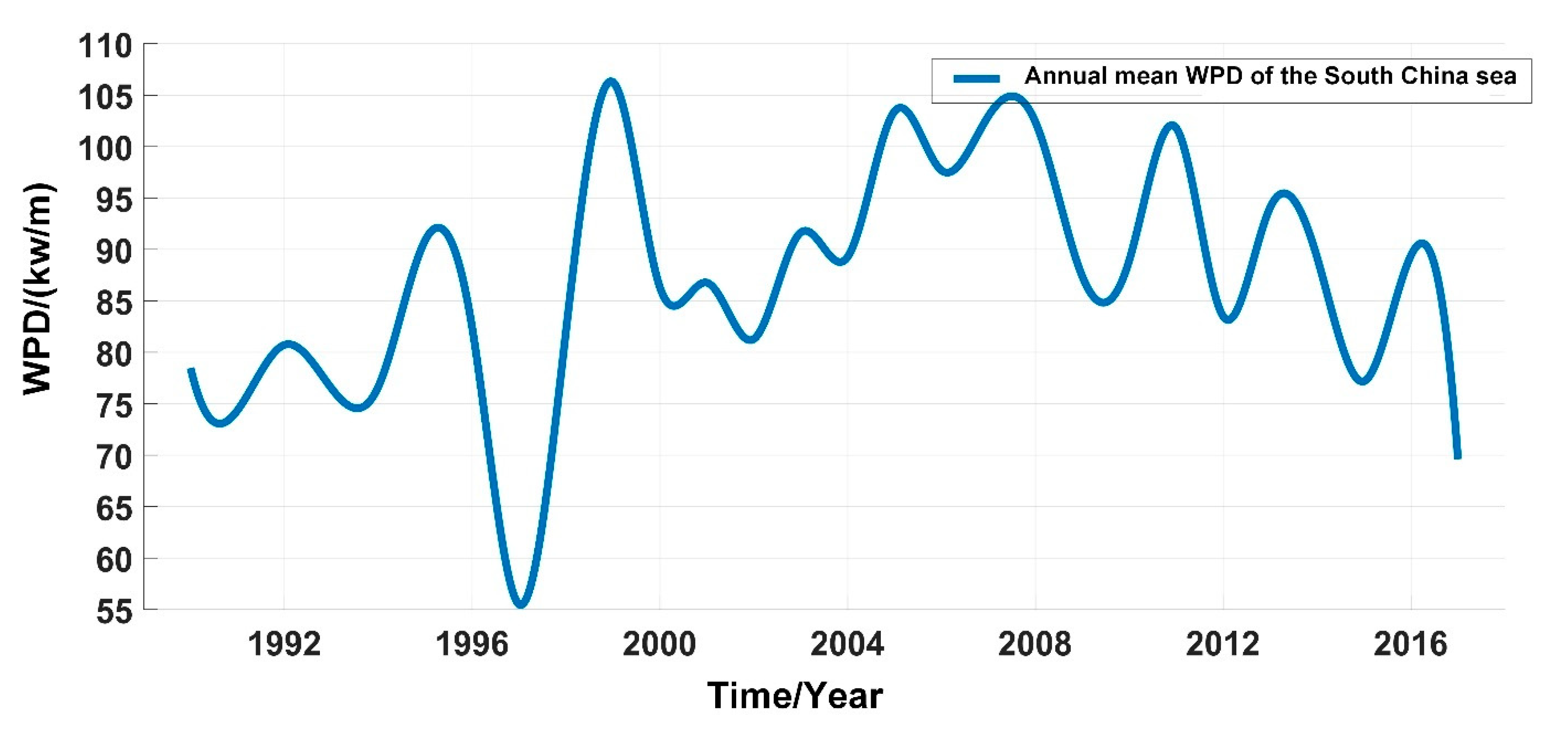
3.1. Annual Variation of WPD in the South China Sea

In this section, the overall WPD variation in the South China Sea is deeply analyzed by means of the MK test, the long-term trend of WPD variation in the South China Sea is comprehensively grasped, and the sources of influence causing the change of WPD in the South China Sea are more accurately analyzed. Figure 6 shows the time variation curve of annual mean WPD in the South China Sea in 28 years.

As shown in Figure 6, the distribution of WPD in the South China Sea in the past 28 years is characterized by “low on the left and high on the right”. That is, a significant increase in WPD occurred, and the main change time was from 1994 to 1998. However, in 1997, the lowest value of WPD occurred in the past 28 years, which was much smaller than that in other years. Meanwhile, the outbreak of the EI Nino phenomenon in the Pacific Ocean has brought a great impact, which increased the overall sea surface water temperature in the South China Sea [14,15]. The EI Nino occurred from 1997 to 1998, and WPD in 1997 was the lowest value in the past 28 years. In the winter of 1998, when EI Nino ended, WPD in the South China Sea began to increase. Therefore, it can be inferred that the variation of WPD value in the South China Sea is likely related to the EI Nino from 1997 to 1998, and it is likely that the sea temperature increase caused by EI Nino [16] and the increase of sea temperature made the WPD value in the South China Sea reach a trough. The MK algorithm was used to test the WPD values of the South China Sea for 28 years, and the trend test chart of WPD was obtained, as shown in Figure 7.

According to the analysis in Figure 7, the MK test results show that the intersection of the two statistics only occurred in 1995, indicating that the abrupt change of energy flux density occurred, while there was no abrupt change in other years. The reason for this result is that 1995 saw the first large-scale increase in the overall WPD, and the average WPD in subsequent years was nearly 93 kW/m. However, after 2000, especially after 2003, UFk began to exceed the positive critical value of 1.96, indicating a significant increase in WPD in this area. This phenomenon continued until 2017, but the growth rate slowed down.

3.2. Trend Analysis of WPD in the Dominant Area of the South China Sea

Shaobo Yang [17] has analyzed the overall change of WPD in the South China Sea, and it is found that there are three areas in the South China Sea where the wave power density is mainly increasing, namely Dongsha Islands, Taiwan Strait, and Luzon Strait. Therefore, this paper analyzes these three areas as the dominant areas of the South China Sea. The selected spatial scale of Dongsha Islands, Taiwan Strait, and Luzon Strait is 115.625° E~117.125° E, 20.625° N~21.375° N; 118.375° E~121.875° E, 23.125° N~25.625° N, and 118.875°~122.875° E, 18.375°~20.375° N respectively. Figure 8 shows the geographic regions of the dominant sea areas in the South China Sea.

In this section, the long-term trend of WPD variation in the dominant sea area of the South China Sea was comprehensively grasped, and the overall WPD variation in the dominant sea area was analyzed by means of the MK test. Figure 9 shows the annual mean WPD of the dominant sea area, and the value of the mean WPD of the dominant sea area was calculated by the sum of the monthly WPD means of each longitude and latitude point in each sea area in that year.

In Figure 9, it is found that the trend change of the sea area of Dongsha Islands is close to that of the Luzon Strait, while the Taiwan Strait is different, mainly manifested in an obvious increasing interval from 2004 to 2008. The MK algorithm was used to test the WPD values of the dominant sea area for 28 years, and the trend test chart of WPD was obtained, as shown in Figure 10.

It can be seen from Figure 9 and Figure 10 that there are some similarities and differences in the variation trends of WPD in the three dominant sea areas. The main similarities between the three sea areas are as follows:

(1)

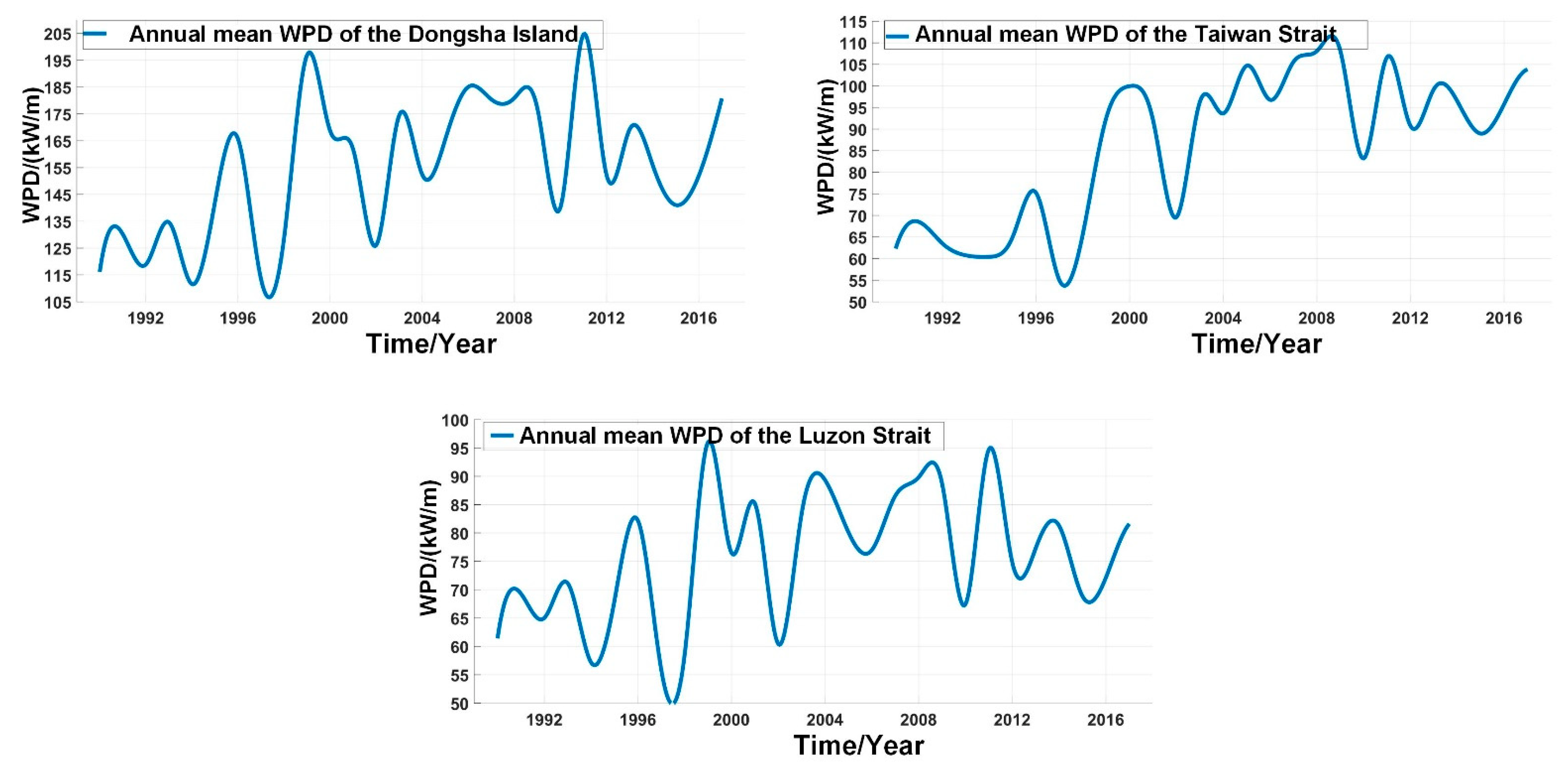
As mentioned above, the strongest EI Nino in the 20th century occurred in the Western Pacific in 1997 [18], which had a great impact on the WPD of the South China Sea. The average annual value of WPD in the three sea areas was the lowest in nearly 30 years. These changes also indicate that the temperature increase caused by EI Nino will have an impact on the WPD value of the South China Sea.

(2)

The peak time of the WPD value from 2007 to 2008 was much higher than that in other years, and the peak time in general years was only about 1 month. Around this time the La Nino phenomenon occurred in the Pacific Ocean, and the time was from August 2007 to May 2008 [19,20]. La Nino usually leads to a decrease in sea temperature, while the WPD value in the South China Sea increased at this time, which proves the relationship between temperature and WPD value change in the South China Sea.

(3)

2011 was another special year for the WPD values of the three sea areas, and the maximum or sub-extreme values of nearly 30 years appeared this year. Dongsha Islands showed the maximum value of 28 years, and the Taiwan Strait and Luzon Strait showed sub-extreme values. According to the data, another La Nina event occurred in the equatorial Middle East Pacific this year. From July 2010 to April 2011, the maximum SST temperature difference appeared in December 2010, reaching −1.5 °C [21], and the rapid seawater cooling resulted in a large increase in the WPD, which again reflected that the change of WPD in the South China Sea may have a strong correlation with the change of seawater temperature.

(4)

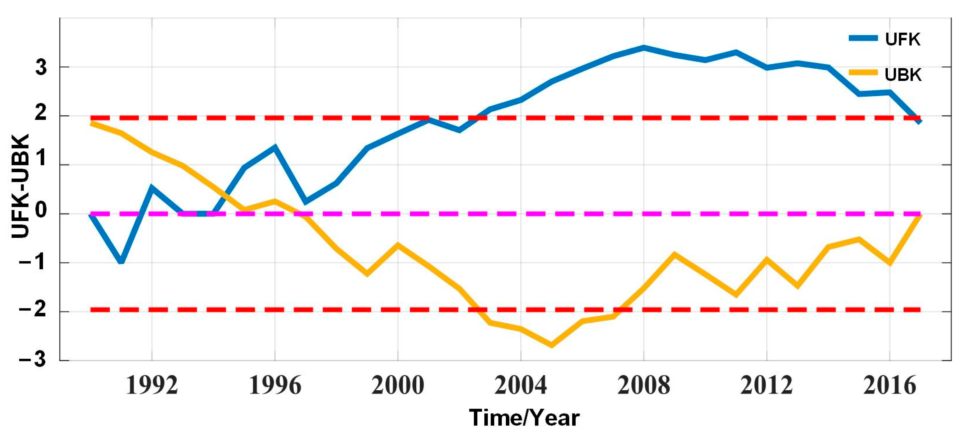
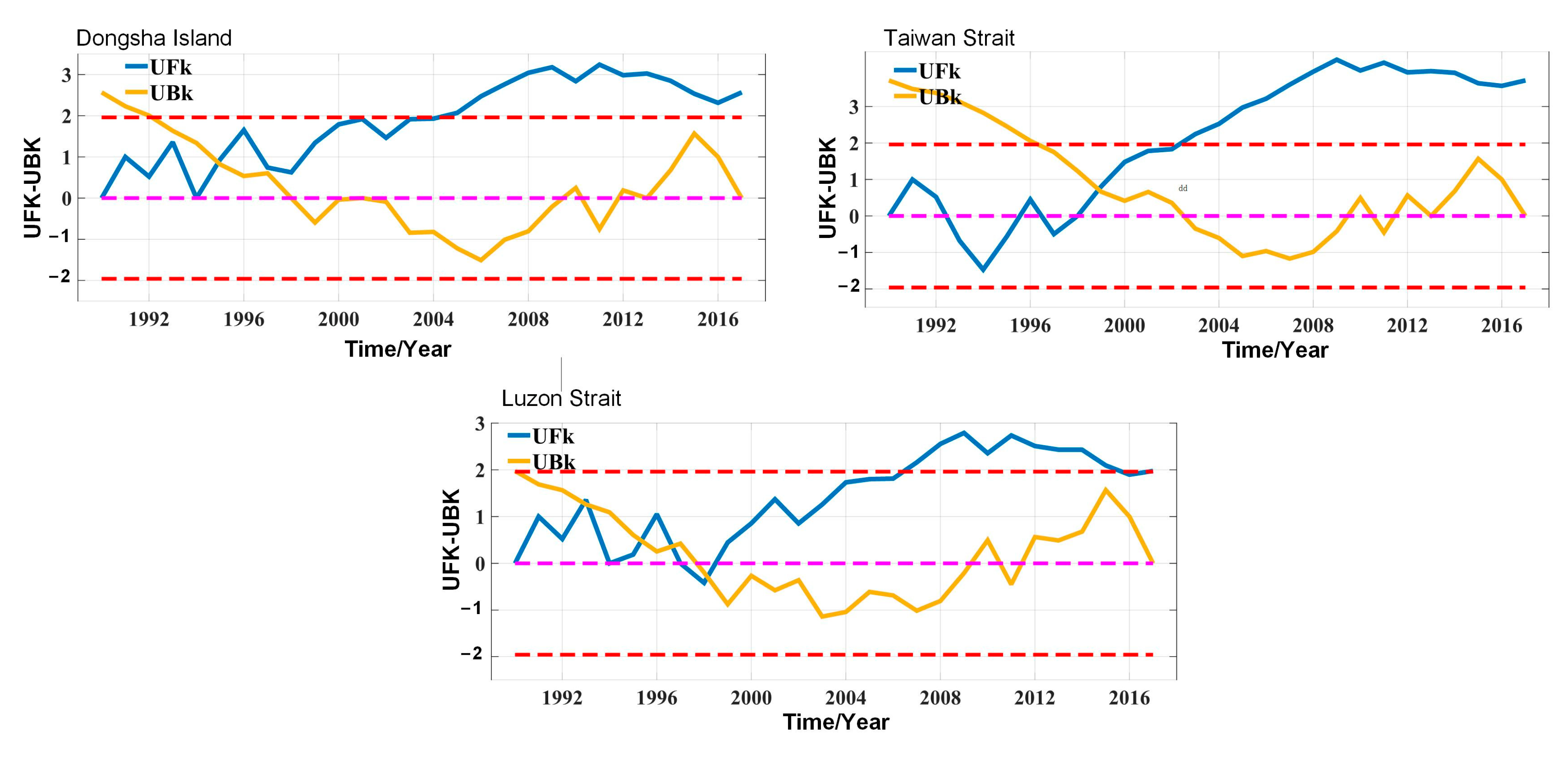
According to the analysis in Figure 10, the WPD growth trend of the three sea areas in the past 30 years kept pace with each other. Before 2004, the growth trend was weak, but after that, the overall growth trend was significantly enhanced. UFK of statistics remained above the critical value until the end of 2017.

The main differences between the three sea areas are as follows:

(1)

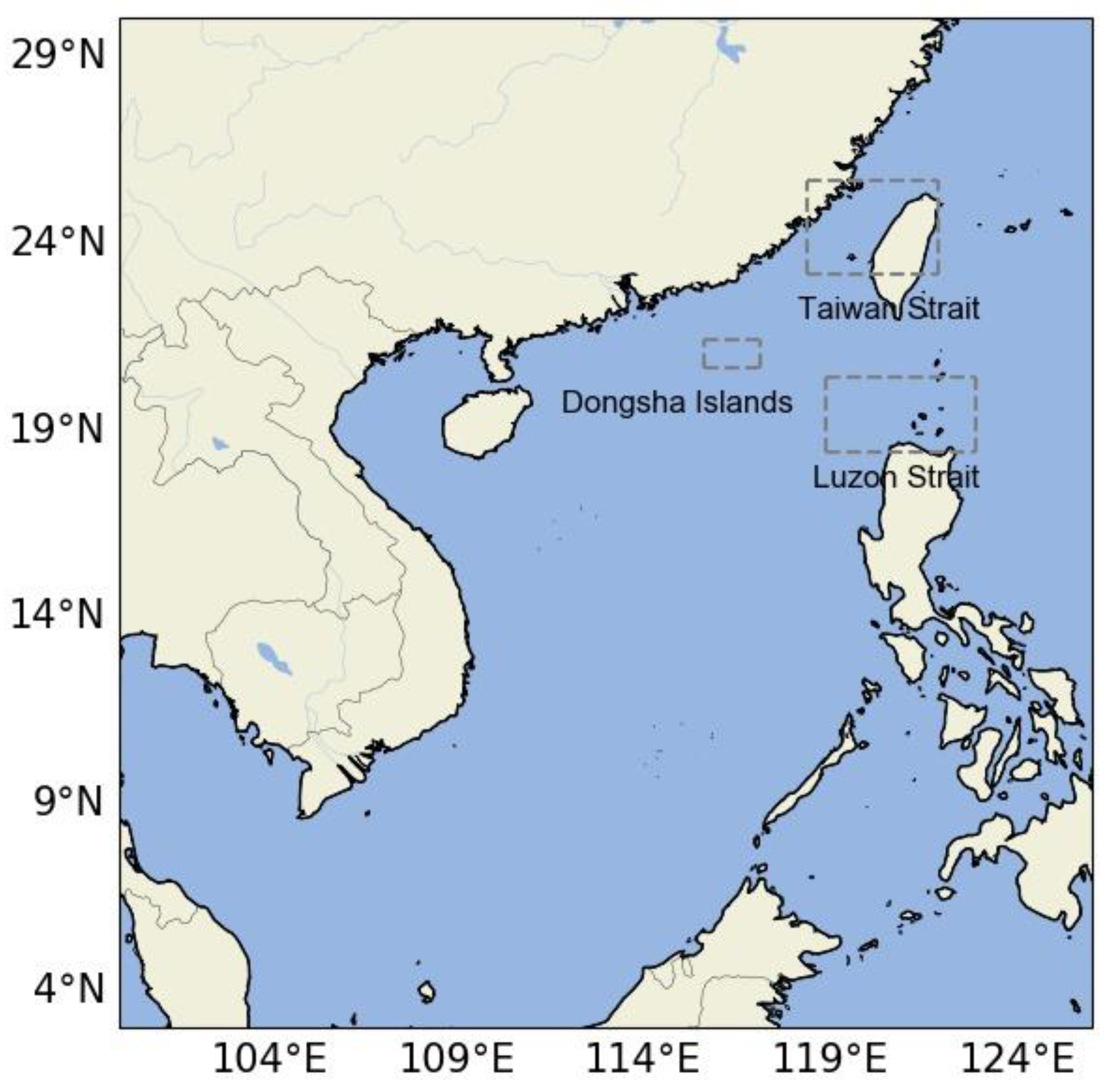
According to Figure 9, the annual WPD value of Dongsha Islands is significantly higher than that of the Taiwan Strait and Luzon Strait, and its value is near twice that of the other two. Considering that the influence of the northeast monsoon in winter is close, the cause of this result may be related to the Marine topography because the Dongsha Islands are mostly surrounded by oceans, while the Luzon Strait and Taiwan Strait are surrounded by a large area of land or islands. It is speculated that the water depth and seawater fluidity may affect the WPD.

(2)

According to the analysis of Figure 10, the abrupt change time of Dongsha Islands is 1994, which is the same as the abrupt change time of the whole South China Sea, and it is the first time of large trend growth, indicating that Dongsha Islands has the greatest impact on the overall trend change of the South China Sea. The abrupt change time in the Taiwan Strait is about January 1999, which is closer to the time when the WPD rebounded sharply after the disappearance of El Nino, but the overall impact on the South China Sea is not as great as that in the Dongsha Sea. The mutation of Luzon Strait was repeated frequently. The reason for the repetition may be that the terrain of Luzon Strait was more complex than that of the former, or the applicability of MK test was not strong under this data condition.

3.3. Exploitable Analysis of WPD in Dominant Sea Area

K.B et al. [22] divided the available WPD into two grades: 2 kW/m (general) and 20 kW/m (rich). Based on this, this paper believes that the WPD value less than 2 kW/m is not suitable for development, between 2 kW/m−20 kW/m is suitable for development, and above 20 kW/m is very suitable for development.

The monthly mean time variation trend of WPD in the dominant sea area is shown in Figure 11, and the value of the mean WPD of the dominant sea area was calculated by the sum of the monthly WPD mean values of each longitude and latitude point in the dominant sea area. In addition, through the evaluation of the 324 months from 1990 to 2017, it is judged that these months belong to Inadequacy, adaptive, or well-suited. The results of the three levels are collected in

Table 2. Statistics of developable months of WPD in dominant sea areas.

	Pratas Island	Taiwan Strait	Luzon Strait
Inadequacy	10	41	70
Adaptive	265	289	260
Well suited	61	6	6

.

As can be seen from Figure 11, the Taiwan Strait and Luzon Strait are suitable for development in all months, while the overall WPD of Dongsha Islands is higher than that of the first two sea areas, and the level of January, November, and December is very suitable for development. Therefore, site selection of the three sea areas is optional from the perspective of energy. On the premise that all three sea areas are suitable for development, the analysis combined with Table 2 shows that the WPD of Dongsha Islands has the highest developable efficiency, and the number of months very suitable for development is 10 times that of the other two, while the WPD of Taiwan Strait has a higher developable value than Luzon Strait, and the number of months unsuitable for development is 30 months less (nearly 10%) than Luzon Strait. Therefore, From the perspective of energy conversion efficiency, the order of development value of the dominant sea area is Dongsha Islands, Taiwan Strait, and Luzon Strait.

However, the strategic value of the Taiwan Strait itself is very high, and the island of Taiwan is the largest island in our country. Therefore, the Taiwan Strait has a particularly prominent position in our maritime security. In contrast, the Dongsha Islands are far from the inland, and the maintenance and construction of energy conversion stations require a large number of costs. Besides being far from the Chinese mainland, the Luzon Strait is also too close to the Philippines and other countries, so it is not suitable for the first construction from the perspective of security and technology. Therefore, Taiwan Strait can play an important role as an energy transfer station in the South China Sea.

4. Conclusions

At present, there are few studies on the long-term changes in wave power density. This paper studied the time variation trend of WPD in the South China Sea and further studies the WPD variation trend of the dominant sea areas in the South China Sea. In this way, the stability of WPD in the South China Sea can be determined, and it is also convenient for the following study of abnormal WPD values in some years. Based on this, the suitable sea area for the development of wave energy and how WPD in the South China Sea is affected by extreme weather were further determined. The analysis results are as follows:

(1)

Extreme weather has a great impact on the change of WPD in the South China Sea. El Nino in 1997, La Nina in 2007, and 2011 all brought subversive changes to WPD in the South China Sea. Moreover, these two extreme weather events are likely to affect the WPD value of the South China Sea by affecting the sea temperature.

(2)

The overall WPD in the South China Sea keeps increasing, with a slight increase before 2004 and a significant increase after 2004; the period of abrupt change in the South China Sea in 28 years was about 1994.

(3)

The trend of the sea area of Dongsha Islands is close to that of the Luzon Strait, while the Taiwan Strait is different, mainly showing an obvious increasing interval from 2004 to 2008. In addition, the annual WPD value of Dongsha Islands is significantly higher than that of the Taiwan Strait and Luzon Strait, and its value is near twice that of the other two.

(4)

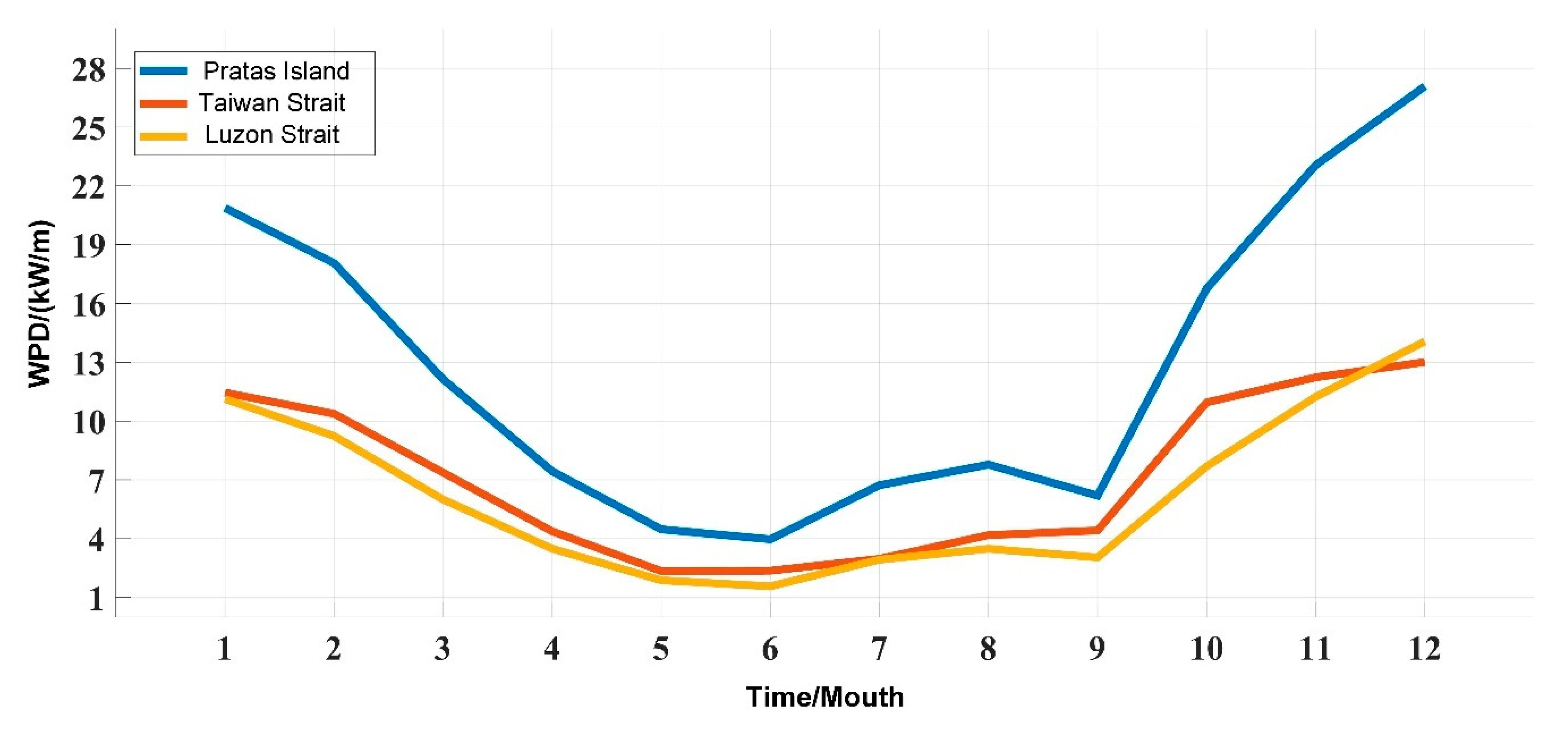
Among the three dominant sea areas, Dongsha Islands has the most exploitable months and the most abundant exploitable WPD resources, followed by Taiwan Strait and Luzon Strait. However, from the perspective of construction, the waters around Taiwan Strait are more suitable as the primary site for energy conversion.

In this paper, the verification of WW3 simulation results is only realized by comparing them with satellite altimeter data. More and more marine observing equipment for obtaining wave data may be applied for comparison with satellite altimeter data to improve the accuracy of WW3 simulation results.

References

1. Thorpe, T.W. A Brief Review of Wave Energy, 1st ed.; Oxford: London, UK, 1999; pp. 133–156. [Google Scholar]
2. Lenee-Bluhm, P.; Paasch, R.; Özkan-Haller, H.T. Characterizing the wave energy resource of the US Pacific Northwest. Renew. Energy 2011, 36, 2106–2119. [Google Scholar] [CrossRef]
3. Barstow, S.; Haug, O.; Krogstad, H. Satellite Altimeter Data in Wave Energy Studies. Ocean Wave Meas. Anal. ASCE 1998, 2, 339–354. [Google Scholar]
4. Wan, Y.; Zhang, J.; Meng, J.M.; Wang, J. A wave energy resource assessment in the China’s seas based on multi-satellite merged radar altimeter data. Acta Oceanol. Sin. 2015, 34, 115–124. [Google Scholar] [CrossRef]
5. Kompor, W.; Ekkawatpanit, C. Assessment of ocean wave energy resource potential in Thailand. Ocean Coast. Manag. 2018, 160, 64–74. [Google Scholar] [CrossRef]
6. Zheng, C.W.; Li, C.Y. Analysis of temporal and spatial characteristics of waves in the Indian Ocean based on ERA-40 wave reanalysis. Appl. Ocean Res. 2017, 63, 217–228. [Google Scholar] [CrossRef]
7. Goncalves, M.; Martinho, P. Wave energy conditions in the western French coast. Renew. Energy 2014, 62, 155–163. [Google Scholar] [CrossRef]
8. Liberti, L.; Carillo, A.; Sannino, G. Wave energy resource assessment in the Mediterranean, the Italian perspective. Renew. Energy 2013, 50, 938–949. [Google Scholar] [CrossRef]
9. Zheng, C.; Zhuang, H.; Li, X.; Li, X. Wind energy and wave energy resources assessment in the East China Sea and South China Sea. Sci. China Technol. Sci. 2012, 55, 163–173. [Google Scholar] [CrossRef]
10. Wang, Z.; Duan, C.; Dong, S. Long-term wind and wave energy resource assessment in the South China sea based on 30-year hindcast data. Ocean Eng. 2018, 163, 58–75. [Google Scholar] [CrossRef]
11. Sam, B.; Jennifer, H.; Mark, H.; Osman, P. Assessing the wave energy converter potential for Australian coastal regions. Renew. Energy 2012, 43, 210–217. [Google Scholar]
12. Henfridsson, U.; Neimane, V.; Strand, K.; Kapper, R.; Bernhoff, H.; Danielsson, O.; Leijon, M.; Sundberg, J.; Thorburn, K.; Ericsson, E.; et al. Wave energy potential in the Baltic Sea and the Danish part of the North Sea, with reflections on the Skagerrak. Renew. Energy 2007, 32, 2069–2084. [Google Scholar] [CrossRef]
13. Rusu, L.; Soares, C.G. Wave energy assessments in the Azores islands. Renew. Energy 2012, 45, 183–196. [Google Scholar] [CrossRef]
14. Zhang, X.; Liang, R. Analysis of weather and meteorological anomalies in the South China Sea in 1997–1998. Mar. Forecast. 2009, 26, 7–13. [Google Scholar]
15. Bao, Y.; Lan, J.; Wang, Y. Anomalous changes in the South China Sea after the 1997/1998 EINino event. Adv. Earth Sci. 2008, 2008, 1027–1036. [Google Scholar]
16. Wang, D.; Xie, Q.; Du, Y.; Wang, W.; Chen, J. 1997–1998 South China Sea warm event. Chin. Sci. Bull. 2002, 2002, 711–716. [Google Scholar]
17. Yang, S.; Zhuang, J.; Xi, L.; Deng, Z.; Zhan, C.; Zheng, C.; Li, X.; Li, H. Long-term variation of the Wave Power Density in the South China Sea over the past 28 years. IEEE Access 2020, 8, 128498–128508. [Google Scholar] [CrossRef]
18. Li, X. Overview of major global climate events in 1997. Meteorological 1998, 1998, 1–4. [Google Scholar]
19. Liang, X.; Guo, Y. Overview of major global weather and climate events in 2007. Meteorological 2008, 34, 113–117. [Google Scholar]
20. Liang, X.; Guo, Y. Overview of major global weather and climate events in 2008. Meteorological 2009, 35, 108–111. [Google Scholar]
21. Si, D.; Li, X.; Re, F.; Xu, L.; Yuan, Y.; Gong, Z. Major global climate events and the causes in 2011. Meteorological 2012, 38, 113–117. [Google Scholar]
22. Kamranzad, B.; Etemad-Shahidi, A.; Chegini, V. Developing an optimum hotspot identifier for wave energy extracting in the northern Persian Gulf. Renew. Energy 2017, 114, 59–71. [Google Scholar] [CrossRef]
Figure 1. Topographic map of the South China Sea.
Jmse 11 00608 g001
Figure 2. Observed and calculated wave height variation trend at the P1 position. The pink line represents the simulated wave height of the CCMP wind field, and the green dotted line represents the observed data of the altimeter.
Jmse 11 00608 g002
Figure 3. Observed and calculated wave height variation trend at the P2 position. The pink line represents the simulated wave height of the CCMP wind field, and the green dotted line represents the observed data of the altimeter.
Jmse 11 00608 g003
Figure 4. Observed and calculated wave height variation trend at the P3 position. The pink line represents the simulated wave height of the CCMP wind field, and the green dotted line represents the observed data of the altimeter.
Jmse 11 00608 g004
Figure 5. Observed and calculated wave height variation trend at the P4 position. The pink line represents the simulated wave height of the CCMP wind field, and the green dotted line represents the observed data of the altimeter.
Jmse 11 00608 g005
Figure 6. Annual variation of WPD in the South China Sea.
Jmse 11 00608 g006
Figure 7. The MK test of annual variation of WPD in the South China Sea.
Jmse 11 00608 g007
Figure 8. The geographic regions of the dominant sea areas.
Jmse 11 00608 g008
Figure 9. Variation trend of WPD in dominant sea area year by year.
Jmse 11 00608 g009
Figure 10. Dominant sea area year-by-year MK test.
Jmse 11 00608 g010
Figure 11. Comparison of monthly WPD values from January to December in dominant sea area.
Jmse 11 00608 g011