A Hybrid Multi-Criteria Decision-Making Framework for Ship-Equipment Suitability Evaluation Using Improved ISM, AHP, and Fuzzy TOPSIS Methods

Abstract

The inherent complexity of large ships makes it challenging to evaluate ship designs systematically and scientifically. Knowledge-based expert systems can be reasonable solutions. However, this problem needs more rationality and better operability, especially in complicated ship-equipment suitability evaluation problems with numerous indicators and complex structures. This paper presents a hybrid multi-criteria decision-making (MCDM) framework to extend the ship-equipment suitability evaluation to group decision-making settings, where individual consistency and group consensus are thoroughly investigated to improve rationality and operability. As a result, an improved Interpretive Structural Modeling (ISM) method is developed to construct the evaluation index systems. Furthermore, based on an applicability analysis of the selected MCDM methods, an improved Analytical Hierarchy Process (AHP) method is proposed to distribute the index weights, and an applicable Fuzzy Technique for Order Preference by Similarity to Ideal Solution (Fuzzy TOPSIS) method is utilized to evaluate and select appropriate ship designs. Finally, a ship-equipment environmental suitability evaluation case is examined. The results indicate that the proposed framework improves the rationality and operability of the decision-making process and provides practical support to decision-makers for the systematic and scientific evaluation of ship designs. Therefore, it can also be applied to other ship design evaluation and selection problems.

1. Introduction

Warship development is a complex, iterative, and multifaceted systems engineering process. Ship-equipment suitability is one of the most challenging design tasks faced by ship designers, which is critical to the operational security and efficiency of shipborne equipment. In the design phase of ship-equipment suitability, scientific evaluation of alternative designs can help identify their strengths and weaknesses and provide ship designers with decision guidance and optimization bases to facilitate improved ship designs [1]. Thus, a scientific evaluation methodology for ship-equipment suitability is significant to developing warships.

Considering the deficiency of the current research on ship-equipment suitability evaluation, we could consider the problem from a more abstract level. Evaluating alternatives can be regarded as a multi-criteria decision-making (MCDM) problem [2,3,4]. In practical problems, the main difficulty is constructing reasonable evaluation index systems and developing scientific evaluation methods.

MCDM methods are currently used in the evaluation, ranking, classification, and selection problems in civil [5,6], marine [7,8,9,10], mechanical [11,12], aerospace [13,14], and many other engineering fields. Numerous approaches have been proposed and applied to various decision problems in different circumstances, including Analytic Hierarchy Process (AHP) [4], Technique for Order Preference by Similarity to an Ideal Solution (TOPSIS) [9], Vlse Kriterijumska Optimizacijia Kompromisno Resenje (VIKOR) [15], Preference Ranking Organization Method for Enrichment Evaluations (PROMETHEE) [16], ELimination Et Choix Traduisant la REalite (ELECTRE) [17], Multi-attribute Utility Theory (MAUT) [18], and many others. However, decision-makers often evaluate criteria performances using linguistic terms instead of determinate values, owing to the suitability of the former for handling imprecise criteria and facilitating the integrated analysis of qualitative and quantitative factors [19,20]. Therefore, MCDM methods have been extensively combined with fuzzy set theory in applications including Fuzzy AHP [8,21], Fuzzy ANP [22], Fuzzy TOPSIS [8], Fuzzy VIKOR [7,23], Fuzzy PROMETHEE [24], Fuzzy ELECTRE [25], Fuzzy evaluation based on distance from average solution (Fuzzy EDAS) [26], and many others to address uncertainty in decision problems. In group decision-making settings, scholars have developed many information fusion operators, such as the bipolar fuzzy aggregation operators [27], q-rung ortho-pair fuzzy aggregation operators [28], Pythagorean fuzzy aggregation operators [29,30], moderator intuitionistic fuzzy aggregation operators [31], etc. These operators can effectively aggregate decision information and have excellent engineering application prospects. In addition, with the rapid development of machine learning and artificial intelligence, intelligent decision-making techniques have been widely used in numerous engineering fields, such as manufacturing [32,33], composite material [34], renewable energy [35], material processing [36], etc.

In addition, extensive research has been conducted on choosing MCDM methods according to two main routes. The first approach [19,37,38,39,40] is used for specific decision problems to preliminarily select several commonly used MCDM methods, evaluate their effectiveness via qualitative and quantitative analysis, and select the appropriate MCDM method. Ranking consistency is the most common and essential criterion [41,42,43,44]. The advantage of this method is that it provides specific recommendations for specific decision problems; however, the rationality of the preliminarily selected MCDM methods still needs to be improved. In the second approach [45,46,47], a generalized MCDM method selection framework is constructed by structuring the characteristics of general decision problems and establishing the matching relationship with the MCDM method properties. The applicable MCDM method is then selected based on the constructed framework. This method not only fully interprets the applicability of the preferred methods but also exhibits strong universality. Nevertheless, when they are applied to specific decision problems, there remains a need to analyze the problem characteristics systematically.

The appropriate distribution of index weights is also another critical area of research interest. Currently, the commonly used weighting methods include the AHP [48], Best-Worst Method (BWM) [49], Entropy method [50], etc., of which the AHP is the most well-established and widely used. However, the complexity of practical problems and the limitations of human cognition makes it nearly impossible to maintain complete consistency in successive pairwise comparisons. Therefore, the application of AHP must focus on verifying acceptable individual consistency. For this reason, in-depth studies have been conducted to improve individual consistency. Bozóki et al. [51] and Negahban [52] investigated several consistency optimization strategies. Temesi [53] proposed an interactive judgment correction method that requires decision-makers’ participation. Xu and Xu [54] proposed an iterative approach to locate the 3-tuples to be modified easily. However, the method does not provide sufficient support for identifying the specific matrix elements to be altered or obtaining the recommended values for the modifiable matrix elements. Cao et al. [55], Kou et al. [56], and Mazurek et al. [57] proposed several iterative algorithms, and Mazurek et al. [58] compared the performances of several algorithms (including those above three) on four indices for measuring the preservation of original expert preferences. Their numerical simulation results indicated that none of the algorithms outperformed all of the others. Given that individual inconsistency should be slightly modified by the judgments that further optimize the inconsistency measure [59], an individual consistency improvement approach that preserves the original expert preferences as much as possible is urgently needed. Moreover, owing to the complexity of index systems, individual consistency improvement approaches should reduce the mental workload to some extent on the premise of ensuring the rationality of the weighting results. In addition, owing to the differences in expert preferences, the application of AHP must also focus on verifying the acceptable group consensus. In AHP-group decision-making (AHP-GDM) settings, individual preference can be aggregated in several ways [60]. MarÍa et al. [61] and Moreno-Jiménez et al. [62] proposed the Consistency Consensus Matrix (CCM) to encourage the search for consensus. Altuzarra et al. [63] proposed a general framework from a Bayesian perspective. Aguarón et al. [64] and Escobar et al. [65] extended the CCM to the precise consensus consistency matrix (PCCM). However, to achieve an acceptable group consensus, these methods often have to throw away much of the original preference information; therefore, it is often difficult for decision-makers to recognize the weighting results.

Although extensive research has been conducted on the development and application of MCDM theory and methods, there needs to be more research devoted to constructing evaluation index systems. Furthermore, when selecting applicable MCDM methods for specific decision problems, the number of alternatives and indicators and distribution of qualitative and quantitative indicators, as well as performance types, measurement scales, and comparison means of criteria performances, should be comprehensively considered in addition to the decision goals [45,46,47]. Therefore, the constructed evaluation index system is a critical foundation for MCDM problems and significantly impacts the MCDM method selection and evaluation decision results.

Logically, the construction of evaluation index systems can be divided into two central issues: (1) identification and selection of reasonable assessment indicators; (2) construction of appropriate hierarchical structures. Currently, the commonly used methods for constructing evaluation index systems include the literature survey method [15,66], the (Fuzzy) Delphi method [67,68,69,70], etc. However, these methods emphasize the identification and selection of assessment indicators, whereas the hierarchical structures are directly given based on expert knowledge, resulting in solid subjective arbitrariness. Moreover, when there are differences in expert opinions, it isn’t easy to effectively aggregate them, quantitatively analyze the degree of group consensus, and efficiently revise the views. Therefore, these methods cannot ensure the rationality of the constructed evaluation index systems and are unsuitable for complex warships.

With the continuous increase in the type and number of shipborne systems and the increasing complexity of the relationships among system elements, there are more challenges to identifying and selecting assessment indicators, determining index weights, and, particularly, evaluating criteria performances. In a word, the increasing complexity of warships has posed growing challenges for ship-equipment suitability evaluation.

To address these problems, this paper aims to present a hybrid MCDM framework for the scientific evaluation of ship-equipment suitability. To fulfill this aim, an improved Interpretive Structural Modeling (ISM) method, which integrates expert judgment aggregation, group consensus verification, and expert judgment modification models, is developed to construct the ship-equipment suitability evaluation index system. The applicability of the selected AHP and Fuzzy TOPSIS methods in ship-equipment suitability evaluation is analyzed systematically to further develop the scientific evaluation decision methods. Then, an improved AHP method, combined with individual consistency improvement, expert preference aggregation, and group consensus verification models, is proposed to distribute the index weights. Furthermore, an applicable Fuzzy TOPSIS method is used to evaluate, rank, and select alternative ship-equipment suitability designs.

The highlights of this paper are as follows:

• A hybrid MCDM framework is developed for the scientific evaluation of ship-equipment suitability.
• A structural modeling method is introduced to construct the ship-equipment suitability evaluation index system.
• The applicability of AHP and Fuzzy TOPSIS methods in ship-equipment suitability evaluation is analyzed systematically.
• Individual consistency and group consensus are thoroughly investigated to improve rationality and operability in ship-equipment suitability evaluation.

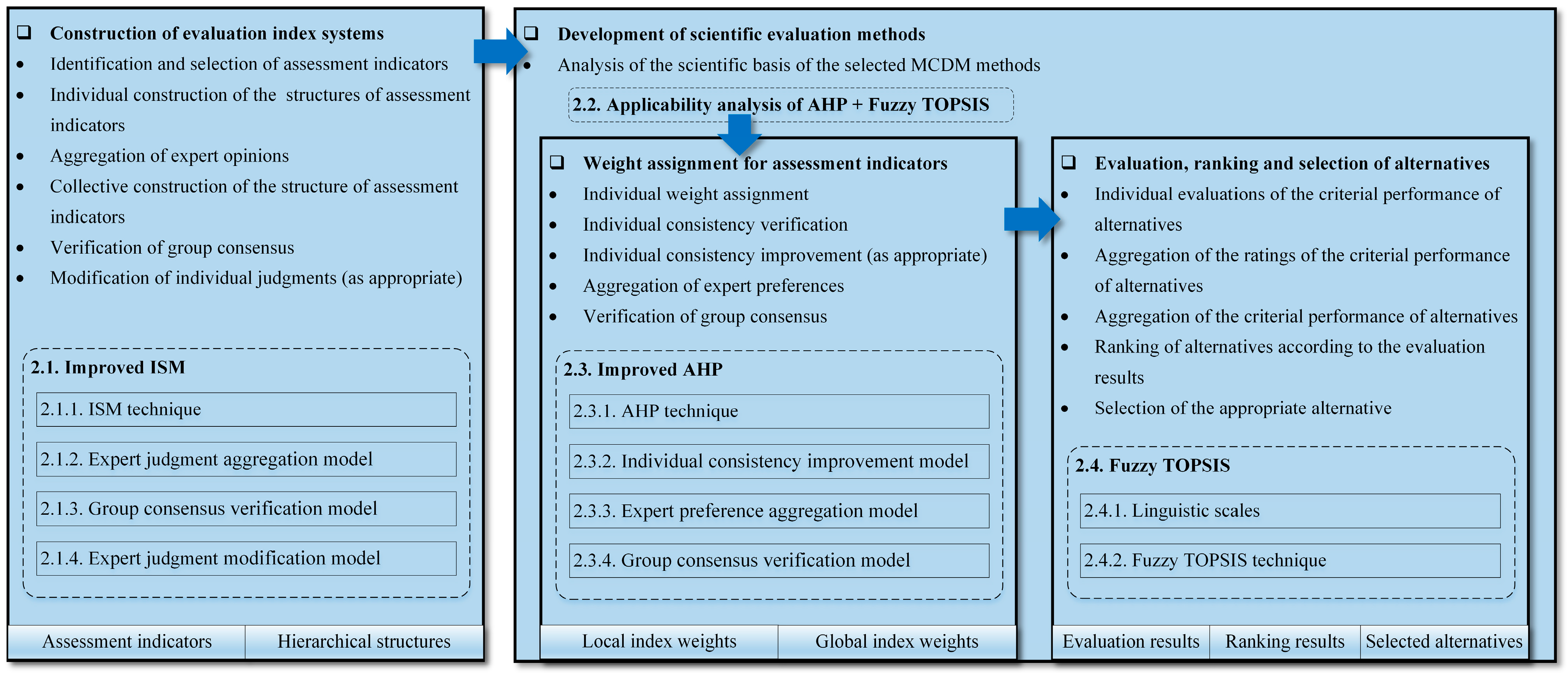
The remaining sections of this paper are organized as follows. The Section 2 introduces the proposed MCDM framework for ship-equipment suitability evaluation. In the Section 3, a case study of ship-equipment environmental suitability evaluation is examined to illustrate the feasibility and effectiveness of the proposed methodology. The Section 4 concludes this paper and outlines future research.

2. Methodology

This section presents a hybrid MCDM framework for ship-equipment suitability evaluation. Figure 1 shows the systematic procedure of the proposed methodology, which consists of four sections. The Section 2.1 presents an improved ISM method to construct the ship-equipment environmental suitability evaluation index system. The Section 2.2 analyzes the scientific basis of the selected MCDM methods. The Section 2.3 presents an improved AHP method to distribute the index weights. Finally, the Section 2.4 uses an applicable Fuzzy TOPSIS method to evaluate, rank, and select alternative ship designs regarding ship-equipment environmental suitability.

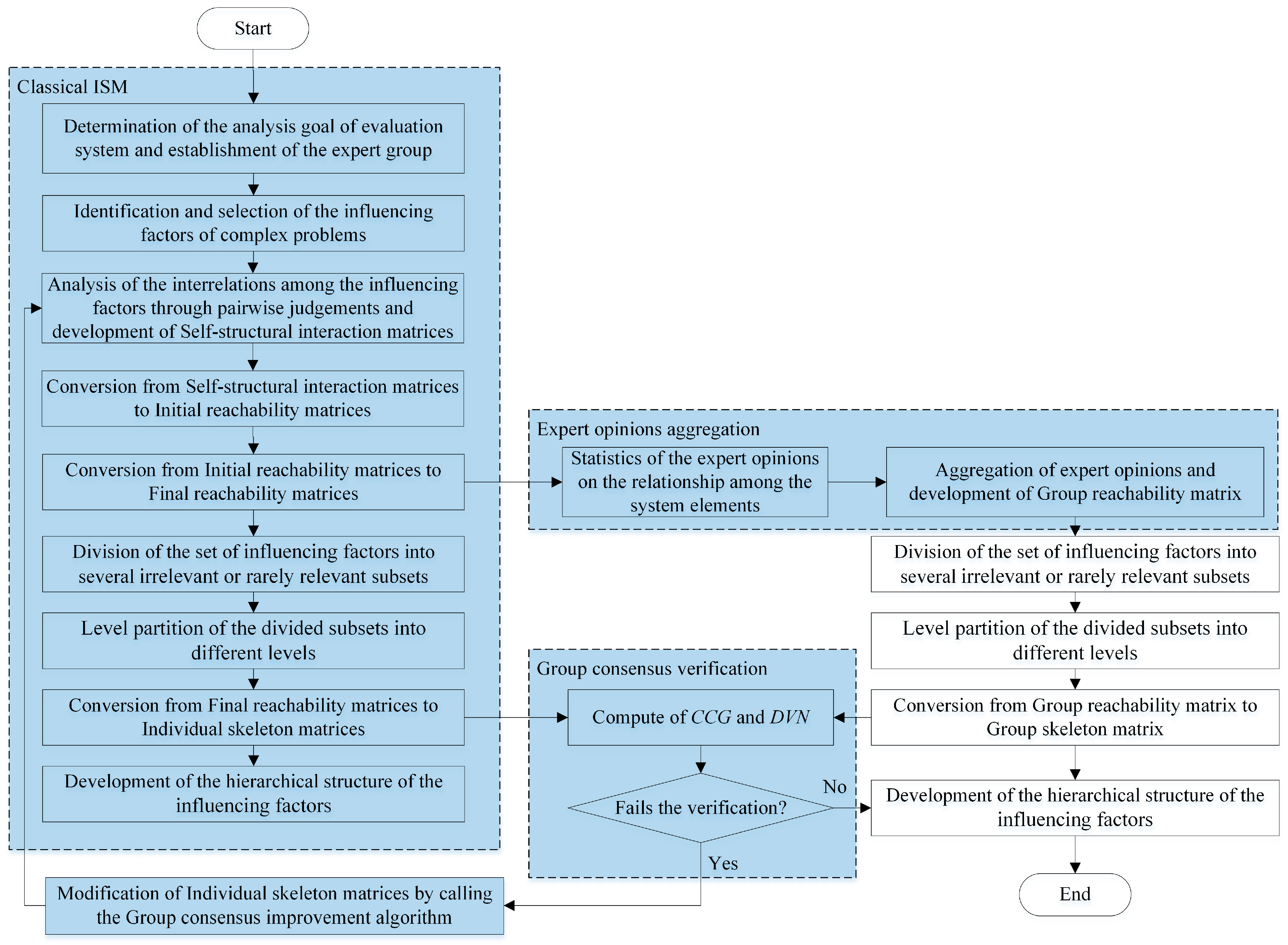
2.1. Improved ISM Technique to Construct Evaluation Index Systems

This section presents an improved ISM method to construct the evaluation index system of ship-equipment environmental suitability. Figure 2 shows the flowchart of the improved ISM method. The classical ISM method is used to construct initial evaluation index systems. In addition, expert judgment aggregation, group consensus verification, and expert judgment modification models are developed to deal with the variances in expert judgments to promote the rationality and operability of evaluation index system construction.

2.1.1. ISM Technique

Warfield [71] developed the ISM method for analyzing the structural problems of complex socio-economic systems. Using expert knowledge, the ISM method can decompose complex systems into influencing factors and their interrelations. Moreover, it can transform complex and confusing interrelations into interpretable, visible, and well-defined hierarchical models [72]. Therefore, the ISM method is regarded as a causal mapping technique for dealing with complicated problems with intricate interrelations and is a standard structural modeling method in the systems engineering field [73,74,75,76].

The ISM method comprises the following steps.

Step 0: Determining the analysis goal and organizing an expert team from ship owners, design institutions, research institutes, shipyards, or equipment manufacturers, $P=\left\{p_1,p_2,\dots ,p_l\right\}$, where $P_k$ denotes the $k$th expert, $k=1,2,\dots ,l$. Let $W^P={\left(w_1^p,w_2^p,\dots ,w_l^p\right)}^T$ be the weight vectors for the experts, which are predetermined based on their professional knowledge, working experiences, educational levels, etc., we have $0<w_k^p<1$ and ${{\displaystyle \sum }}_{k=1}^l{w}_k^p=1$.

Step 1: Identification and selection of influencing factors, $X=\left\{x_1,x_2,\dots ,x_n\right\}$, where $X_i$ denotes the $i$th factor, $i=1,2,\dots ,n$.

Step 2: Development of a Self-structural interaction matrix (SSIM, $O$) based on pairwise judgments on the interrelations among influencing factors.

$$O=\left[\begin{array}{cc}\begin{array}{cc}{o}_{11}& o_{12}\\ & o_{22}\end{array}& \begin{array}{cc}\cdots & o_{1n}\\ \cdots & o_{2n}\end{array}\\ \begin{array}{cc}& \\ & \end{array}& \begin{array}{cc}\ddots & ⋮\\ & o_{nn}\end{array}\end{array}\right],$$

(1)

where $o_{ij}$ denotes the interrelations between factors $X_i$ and $X_j$. The interrelations are expressed using the following four symbols: (1) $>$ refers to factor $X_i$ affects $X_j$ but not vice versa; (2) $<$ refers to factor $X_i$ is affected by $X_j$ but not vice versa; (3) $\sim$ refers to factor $X_i$ affects $X_j$ and vice versa; (4) $\times$ refers to factor $X_i$ does not affect $X_j$ and vice versa. To facilitate modeling and computation, we suppose that factor $X_i$ affects itself, i.e., $o_{ii}=\sim$.

Step 3: Transformation of the SSIM to an initial reachability matrix (IRM, $A$).

$$A=\left[\begin{array}{cc}\begin{array}{cc}{a}_{11}& a_{12}\\ a_{21}& a_{22}\end{array}& \begin{array}{cc}\cdots & a_{1n}\\ \cdots & a_{2n}\end{array}\\ \begin{array}{cc}⋮& ⋮\\ a_{n1}& a_{n2}\end{array}& \begin{array}{cc}\ddots & ⋮\\ \cdots & a_{nn}\end{array}\end{array}\right]$$

(2)

The conversion rules are as follows:

(1)

If $o_{ij}=>$, then $a_{ij}=1$ and $a_{ji}=0$;

(2)

If $o_{ij}=<$, then $a_{ij}=0$ and $a_{ji}=1$;

(3)

If $o_{ij}=\sim$, then $a_{ij}=a_{ji}=1$;

(4)

If $o_{ij}=\times$, then $a_{ij}=a_{ji}=0$.

Step 4

Transformation of the IRM to a final reachability matrix (FRM, $R={\left[r_{ij}\right]}_{n\times n}$) using transitivity rules.

$$R=A{\displaystyle \cup }{A}^2{\displaystyle \cup }\dots {\displaystyle \cup }{A}^n$$

(3)

Step 5

Division of the influencing factors into several irrelevant or rarely relevant subsets. The top-level factors ($X_i$) of the divided subsets are identified using Equation (4), with their antecedent sets $D\left(x_i\right)$ comprising the irrelevant or rarely relevant subsets.

$$\left\{x_i|L\left(x_i\right)=L\left(x_i\right){\displaystyle \cap }D\left(x_i\right), x_i\in X\right\},$$

(4)

where $L\left(x_i\right)$ denotes the reachability set of factors $X_i$, including the factors that are affected by $X_i$ and $D\left(x_i\right)$ denotes the antecedent set of factors $X_i$, including the factors that affect $X_i$.

Step 6

Partitioning of the divided subsets into different levels. The top-level factors of the divided subsets are eliminated first; then, step 5 is repeated to identify the factors in the subordinate level until all the factors complete the level partition.

Step 7

Transformation of the FRM to a skeleton matrix, $S={\left[s_{ij}\right]}_{n\times n}$. The inducing elements that represent the indirect interrelations among influencing factors are identified and eliminated using Equations (5) and (6).

$$f_{ij}=\{\begin{array}{cc}\underset{\begin{array}{c}h=1\\ h\ne i,j\end{array}}{\overset{n}{{\displaystyle \vee }}}\left(r_{ih}\wedge r_{hj}\right)& if r_{ij}=1\\ 0& if r_{ij}=0\end{array},$$

(5)

$$s_{ij}=\{\begin{array}{cc}1& if r_{ij}=1\wedge f_{ij}=0\\ 0& if f_{ij}=0\end{array},$$

(6)

where $f_{ij}$ denotes the property of $r_{ij}$. If $f_{ij}=1$, $r_{ij}$ is an inducing element, while $f_{ij}=0$, $r_{ij}$ is not an inducing element.

Step 8

Development of the digraph of influencing factors according to the divided subsets, partitioned levels, and converted skeleton matrix.

2.1.2. Expert Judgment Aggregation

When more than one expert is involved in constructing evaluation index systems, the opinions of different experts should be considered and aggregated. Thus, an expert judgment aggregation model is proposed as follows.

Step 1: Statistics of the expert judgments on the interrelations among influencing factors using Equations (7) and (8), with the statistical results expressed as a two-tuple matrix, $W={[w_{ij}^1,w_{ij}^0]}_{n\times n}$.

$$w_{ij}^1={{\displaystyle \sum }}_{k=1}^l{w}_k^p, if r_{ij}^k=1,$$

(7)

$$w_{ij}^0={{\displaystyle \sum }}_{k=1}^l{w}_k^p, if r_{ij}^k=0,$$

(8)

where $w_{ij}^1$ denotes the sum of the weights of experts who agree that factor $X_i$ affects $X_j$ and $w_{ij}^0$ represents the sum of the weights of experts who agree that factor $X_i$ does not affect $X_j$. Therefore, the sum of $w_{ij}^1$ and $w_{ij}^0$ is equal to 1.

Step 2: Aggregation of expert judgments using Equation (9) and development of a group reachability matrix, $B={\left[b_{ij}\right]}_{n\times n}$.

$$b_{ij}=\{\begin{array}{cc}1& if w_{ij}^1\ge t\\ 0& otherwise\end{array}$$

(9)

where $t$ is the predetermined threshold for aggregating expert judgments, $t\in \left[0,1\right]$. The value of $t$ can be subjectively determined by the expert group or a highly experienced expert.

2.1.3. Group Consensus Verification

To evaluate the rationality of expert judgment aggregation, two novel indices are proposed to measure the degree of group consensus between the group skeleton matrix (GSM, $S_B$) and the initial individual skeleton matrices (SSM, $S_k$).

• The comparability coefficient for the expert group (CCG) is given as

$$CCG\left(S_B\right)={{\displaystyle \sum }}_{k=1}^l{w}_k^p·CCG\left(S_k\right),$$

(10)

where

$$CCG\left(S_k\right)=\frac{1}{n}{{\displaystyle \sum }}_{i=1}^n{J}_k^{x_i},$$

(11)

$$J_k^{x_i}=\frac{1}{2}\left(J\left(S_k^{r_i}/S_B^{r_i}\right)+J\left(S_k^{c_i}/S_B^{c_i}\right)\right),$$

(12)

and

$$J\left(S_k^{(·)}/S_B^{(·)}\right)=\frac{\left|S_k^{(·)}{\displaystyle \bigcap }{S}_B^{(·)}\right|}{\left|S_k^{(·)}{\displaystyle \bigcup }{S}_B^{(·)}\right|}.$$

(13)

where $r_i$ ($c_i$) denotes the subscript of the $i$th row (column) vector of the skeleton matrices regarding factor $X_i$; $S_k^{(·)}$ denotes the row ($S_k^{r_i}$)/column ($S_k^{c_i}$) vector of the $k$th SSM $S_k$; $S_B^{(·)}$ denotes the row ($S_B^{r_i}$)/column ($S_B^{c_i}$) vector of the GSM $S_B$. $J\left(S_k^{r_i}/S_B^{r_i}\right)$ is defined to measure the similarity of the two-row vectors ($S_k^{r_i}$, $S_B^{r_i}$) regarding factor $X_i$, $J\left(S_k^{c_i}/S_B^{c_i}\right)$ is defined to measure the similarity of the two-column vectors ($S_k^{c_i}$, $S_B^{c_i}$) of factor $X_i$, and $J_k^{x_i}$ is defined to measure the average similarity of the four vectors ($S_k^{r_i}$ and $S_B^{r_i}$, $S_k^{c_i}$ and $S_B^{c_i}$) regarding factor $X_i$. $CCG\left(S_k\right)$ is defined to measure the overall cardinal consensus between the two skeleton matrices $S_k$ and $S_B$. $CCG\left(S_B\right)$ is defined to measure the average cardinal consensus among all the skeleton matrices.

The comparability between two vectors is calculated using the Jaccard similarity coefficient. Thus, the larger the value of $CCG\left(S_k\right)$, the higher the cardinal consensus level of expert $P_k$. Let $\overline{CCG}$ be the predetermined threshold. If $CCG\left(S_k\right)\ge \overline{CCG}$, then the GSM $S_B$ has acceptable cardinal consensus with the SSM $S_k$; if $CCG\left(S_k\right)\ge \overline{CCG}$ for all the GSMs, acceptable cardinal group consensus is achieved by the expert group.

• The direction violation number for the expert group (DVN) is given as

$$DVN\left(S_B\right)={{\displaystyle \sum }}_{k=1}^l{w}_k^p·DVN\left(S_k\right),$$

(14)

where

$$DVN\left(S_k\right)=\frac{1}{n^2}{{\displaystyle \sum }}_{i=1}^n{{\displaystyle \sum }}_{j=1}^n{I}_{ij}\left(S_k/S_B\right),$$

(15)

and

$$I_{ij}\left(S_k/S_B\right)=\{\begin{array}{cc}1& if s_{ij}^B=s_{ij}^k\\ 0& if s_{ij}^B\ne s_{ij}^k\end{array},$$

(16)

where $I_{ij}\left(S_k/S_B\right)$ is defined to measure the difference in matrix elements $s_{ij}^k$ and $s_{ij}^B$. $DVN\left(S_k\right)$ is defined to measure the overall ordinal consensus between the two skeleton matrices $S_k$ and $S_B$. $DVN\left(S_B\right)$ is defined to measure the average ordinal consensus among all the skeleton matrices.

The larger the values of $DVN\left(S_k\right)$, the higher the ordinal consensus levels of expert $P_k$. Let $\overline{DVN}$ be the predetermined threshold. If $DVN\left(S_k\right)\ge \overline{DVN}$, then the GSM $S_B$ has acceptable ordinal consensus with the SSM $S_k$, and if $DVN\left(S_k\right)\ge \overline{DVN}$ for all the SSMs, acceptable ordinal group consensus is achieved by the expert group.

The value of $\overline{CCG}$ and $\overline{DVN}$ can be subjectively determined by the expert group or a highly experienced expert.

2.1.4. Expert Judgment Modification

If an acceptable group consensus is not achieved, the experts should be organized to review their judgments. Based on the SSMs, this section presents a group consensus improvement algorithm (see Figure 3 and Algorithm 1). This interactive iterative algorithm provides experts with critical information support, including the factors and vectors to be reviewed and the elements (interrelations) to be modified.

The group consensus improvement algorithm is as follows.

Algorithm 1. Group consensus improvement algorithm.

Input: SSIM $O_k$   Output: The modified SSM $S_k^{\prime }$, the modified SSIM $O_k^{\prime }$, the associated value $CCG\left(S_k^{\prime }\right)$ and $DVN\left(S_k^{\prime }\right)$      Step 0. Suppose $r_i$ ($c_i$) denotes the subscript of the row (column) vector corresponding to $x_i\in X$ in the skeleton matrices, $S^{r_i}$ ($S^{c_i}$) denotes the row (column) vector corresponding to $x_i\in X$ in the skeleton matrices. Let $t_i=\left\{r_i,c_i\right\}$.   Step 1. Compute $J\left(S_k^{r_i}/S_B^{r_i}\right)$, $J\left(S_k^{c_i}/S_B^{c_i}\right)$ and $J_k^{x_i}$ for all $x_i\in X$.   Step 2. Choose the factor $x_i^{\prime }$ for which $J_k^{x_i}$ has the largest value, let $x_i=x_i^{\prime }$.   Step 3. Choose the subscript $t_i^{\prime }$ for which $J\left(S_k^{t_i}/S_B^{t_i}\right)$ has the largest value, if $J\left(S_k^{r_i}/S_B^{r_i}\right)=J\left(S_k^{c_i}/S_B^{c_i}\right)$, use $t_i^{\prime }=r_i$ and let $t_i=t_i^{\prime }$.   Step 4. Suppose $K=\left\{\left(r,s\right)\right\}$ denotes the index set of the elements of the vector corresponding to $t_i$ in the skeleton matrices. Let $\left(i,j\right)=\left(r,s\right)$, compute $I_{ij}\left(S_k/S_B\right)$ for all $\left(i,j\right)\in K$. Let $L=\left\{\left(i,j\right):I_{ij}\left(S_k/S_B\right)=0\right\}$.   Step 5. Choose the subscript $\left(i^{\prime },j^{\prime }\right)$, i.e., the first $\left(i,j\right)\in L$, let $\left(i,j\right)=\left(i^{\prime },j^{\prime }\right)$.   Step 6. If expert $P_k$ agrees to revise the interrelation $s_{ij}^k$, update the individual skeleton matrix $S_k$ with new values $s_{ij}^k=s_{ij}^B$, update $L=L\backslash \left(i^{\prime },j^{\prime }\right)$ and proceed to Step 7. Otherwise, update $L=L\backslash \left(i^{\prime },j^{\prime }\right)$ and proceed to Step 5.   Step 7. Calculate $CCG\left(S_k^{\prime }\right)$ and $DVN\left(S_k^{\prime }\right)$.   (a) If $CCG\left(S_k^{\prime }\right)\ge \overline{CCG}$ and $DVN\left(S_k^{\prime }\right)\ge \overline{DVN}$, update SSIM $O_k$ with the modified interrelations, and provide $O_k^{\prime }$, $S_k^{\prime }$, $CCG\left(S_k^{\prime }\right)$ and $DVN\left(S_k^{\prime }\right)$.   (b) Otherwise, if $K\ne \varnothing$, repeat Steps 5 through 7.   (c) Otherwise, update $t_i=t_i\backslash t_i^{\prime }$, if $t_i\ne \varnothing$, repeat Steps 3 through 7.   (d) Otherwise, update $X=X\backslash x_i^{\prime }$, if $X\ne \varnothing$, repeat Steps 2 through 7

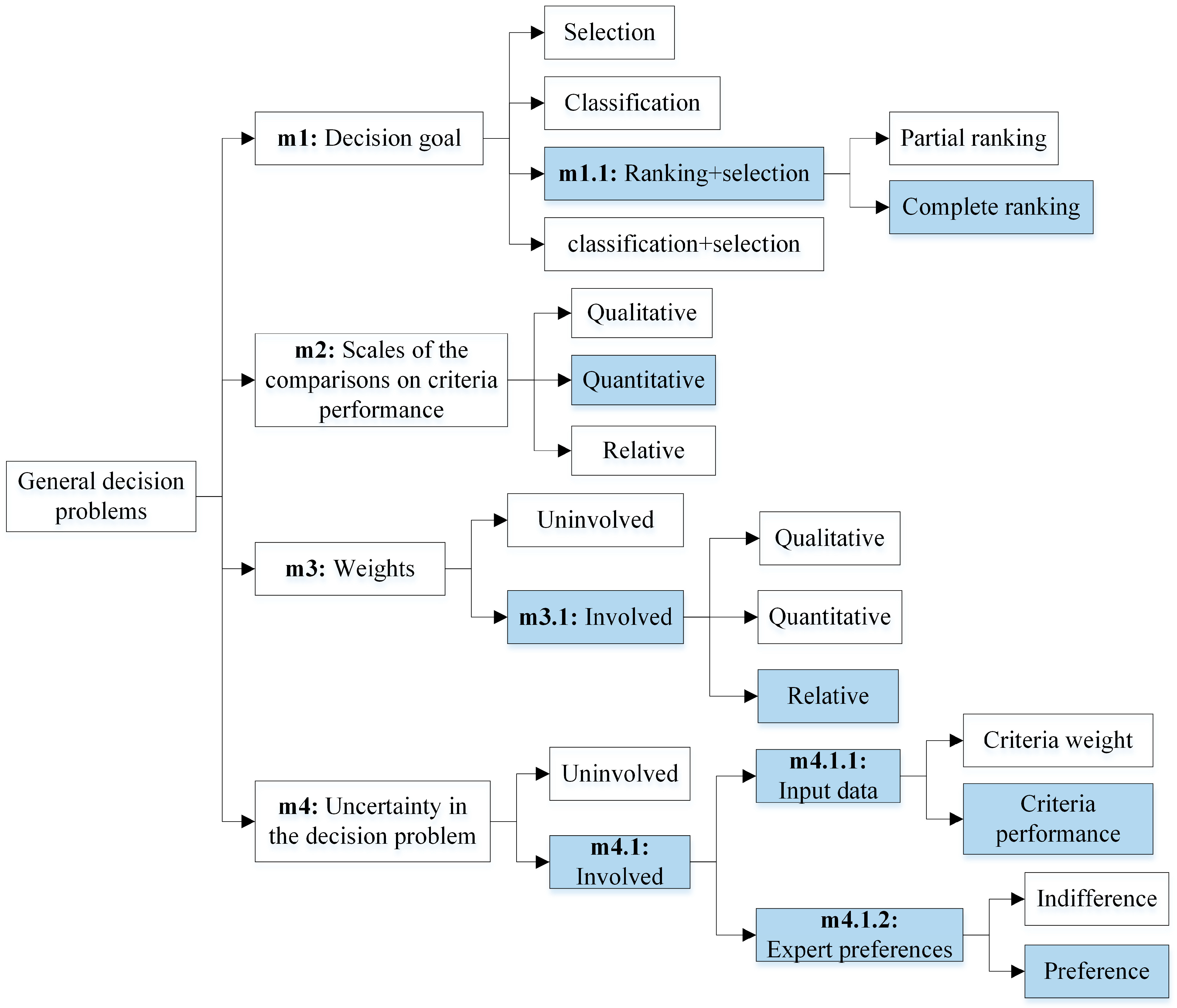
2.2. Applicability Analysis of AHP and Fuzzy TOPSIS

This section systematically analyzes the scientific basis of the selected AHP and Fuzzy TOPSIS methods. The characteristics of general decision problems (see Figure 4) can be described using several descriptors along different dimensions [35]. As a specific instance of general decision problems, some of these descriptors can also describe ship-equipment suitability evaluation. In ship-equipment suitability evaluation:

(1) The decision goal is to evaluate, rank, and select alternative ship-equipment suitability designs. Complete rankings should be performed according to evaluation results to facilitate a comparative analysis of criteria performances among diverse ship designs or within a single design.

(2) For quantitative indicators, criteria performances of alternative ship-equipment suitability designs usually involve quantitative comparisons. For qualitative indicators, criteria performances need to be initially quantified based on qualitative ratings and then compared similarly to quantitative indicators.

(3) It is worth assigning appropriate weights for assessment indicators to measure the importance of differences to overall objectives. Furthermore, relative comparisons are typically used to achieve higher rationality in ship-equipment suitability evaluation.

(4) More importantly, the inherent complexity of warships often makes it difficult to evaluate and compare some criteria performances. Thus, empirical assessments based on expert knowledge can be acceptable solutions. However, such empirical judgments may be somewhat uncertain, especially regarding the criteria performances and expert preferences.

The characteristics of ship-equipment suitability evaluation and the properties of the selected AHP and Fuzzy TOPSIS methods are presented in

Table 1. Problem characteristics and method properties.

	${\mathit{m}}_1$	${\mathit{m}}_{1.1}$	${\mathit{m}}_2$	${\mathit{m}}_3$	${\mathit{m}}_{3.1}$	${\mathit{m}}_4$	${\mathit{m}}_{4.1}$	${\mathit{m}}_{\mathrm{4.1.1}}$	${\mathit{m}}_{\mathrm{4.1.2}}$
Characteristics of ship-equipment suitability evaluation	3	2	2	2	3	2	1,2	2	2
Properties of AHP and Fuzzy TOPSIS methods	3	2	2	2	3	2	1,2	2	2

. It is seen from Table 1 that the properties of the selected MCDM methods match entirely the characteristics of the specific evaluation problem, which illustrates the applicability of AHP and Fuzzy TOPSIS methods in ship-equipment suitability evaluation.

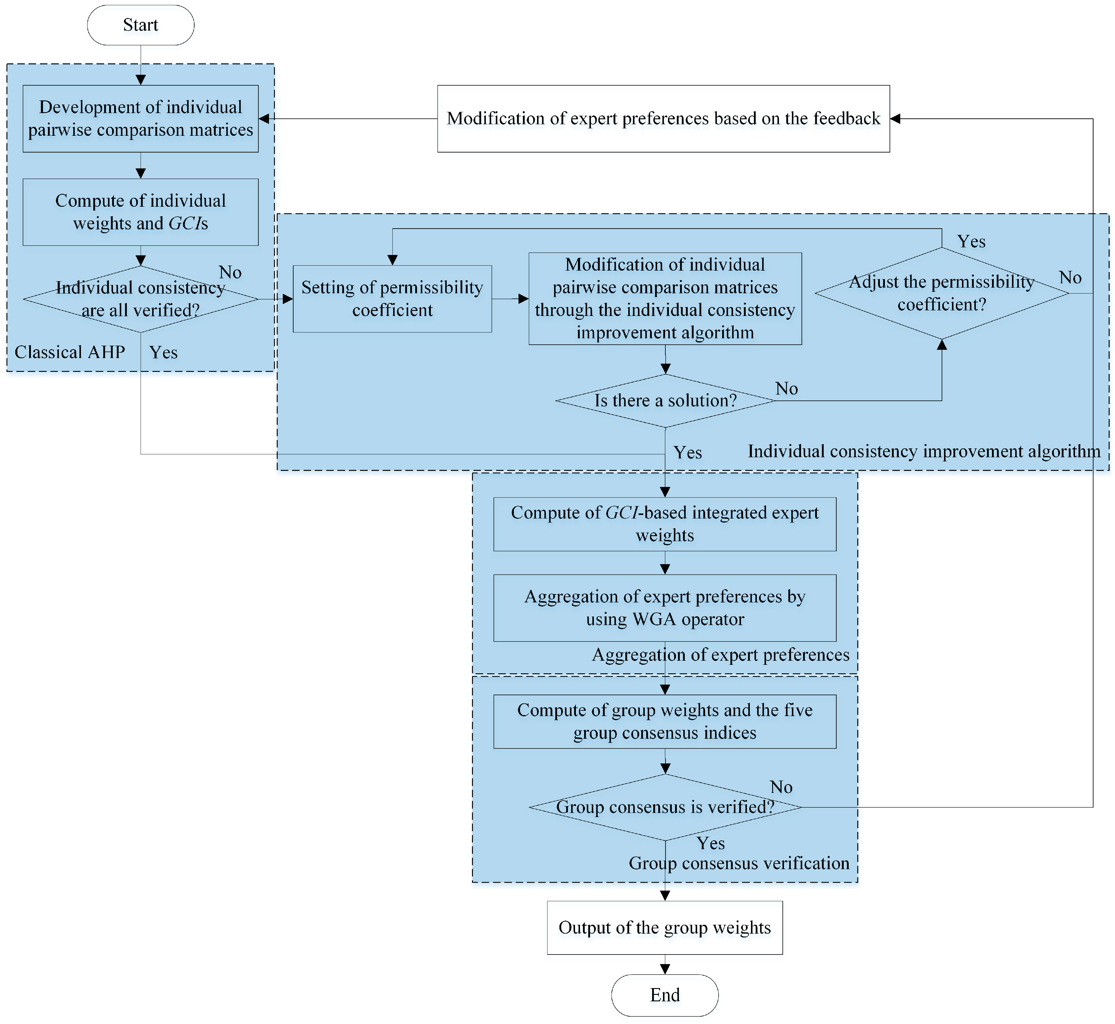
2.3. Improved AHP Technique to Distribute Index Weights

This section presents an improved AHP method (see Figure 5), which integrates individual consistency improvement, expert preference aggregation, and group consensus verification models, to distribute the index weights.

2.3.1. AHP Technique

Saaty [48] developed the AHP method based on pairwise comparisons. The relative importance of each factor against the others is scored based on expert knowledge, with the priority intensity usually scaled by $\left\{\frac{1}{9},\frac{1}{8},\dots ,\frac{1}{2},1,2,\dots ,9\right\}$. Let ${\rm X}=\left\{x_1,x_2,\dots ,x_n\right\}$ be the assessment indicators, the measurement scales of importance intensity and their descriptions are shown in

Table 2. Measurement scales of importance intensity and their descriptions.

Intensity of Importance	Definition
1	$X_i$ and $X_j$ contribute equally to the objective.
3	Experience and knowledge slightly favor $X_i$ over $X_j$.
5	Experience and knowledge strongly favor $X_i$ over $X_j$.
7	$X_i$ is strongly favored, and its dominance is demonstrated in practice.
9	The evidence favoring $X_i$ over $X_j$ is of the highest possible order of affirmation.
2,4,6,8	Intermediate values between the two adjacent judgments
Reciprocals of the above nonzero	If $X_i$ has one of the aforementioned nonzero values, $a_{ij}$ is assigned to it when compared to $X_j$. Thus, $X_j$ has a reciprocal value, $a_{ji}=1/a_{ij}$, when compared to $X_i$.

.

The positive reciprocal judgment matrix, $A={\left[a_{ij}\right]}_{n\times n}$, is constructed based on Table 2 as follows.

$$A=\left[\begin{array}{cccc}1& a_{12}& \cdots & a_{1n}\\ 1/a_{12}& 1& \cdots & a_{2n}\\ ⋮& ⋮& \ddots & ⋮\\ 1/a_{1n}& 1/a_{2n}& \cdots & 1\end{array}\right]$$

(17)

where $a_{ij}$ represents the priority intensity of $X_i$ over $X_j$.

In classical AHP, the eigenvalue method (EVM) is used to compute the weights of the assessment indicators [48]. Recently, owing to its psychological, mathematical, and statistical properties, the Row Geometric Mean (RGM) method [77] has gained popularity in the scientific community and is recognized as an alternative to the EVM [78]. The criterion weight is calculated using Equations (18) and (19).

$$w_i=w_i^{\prime }/{{\displaystyle \sum }}_{j=1}^n{w}_j^{\prime },$$

(18)

$$w_i^{\prime }={{\displaystyle \prod }}_{j=1}^n{\left(a_{ij}\right)}^{1/n}.$$

(19)

The consistency index corresponding to the RGM is the geometric consistency index (GCI) [79], which is calculated as

$$GCI=\frac{2}{\left(n-1\right)\left(n-2\right)}{{\displaystyle \sum }}_{i<j}lo{g}^2{e}_{ij},$$

(20)

where $e_{ij}=a_{ij}{w}_j/w_i$, $w={\left(w_i\right)}_{n\times 1}$ is the weight vector derived from the judgment matrix $A$.

Let $\overline{GCI}$ be the predetermined threshold; its values for judgment matrices of different dimensions are shown in

Table 3. Thresholds of GCI.

$\mathit{n}$	$\overline{\mathit{G}\mathit{C}\mathit{I}}$
3	0.31
4	0.35
>4	0.37

[79]. If $GCI\left(A\right)<\overline{GCI}$, then the judgment matrix $A$ is of acceptable consistency. Otherwise, the judgment matrix $A$ fails the consistency verification.

2.3.2. Individual Consistency Improvement

In AHP, the rationality of the weighting results depends mainly on the consistency level of the expert judgments. Therefore, this section presents a GCI-based individual consistency improvement model [78]. It can provide experts with critical information support, including the judgments to be reviewed, the directions to be adjusted, and the values to be modified.

The GCI-based individual consistency improvement algorithm (see Figure 6 and Algorithm 2) is outlined as follows; a detailed derivation and proof can be found in [78].

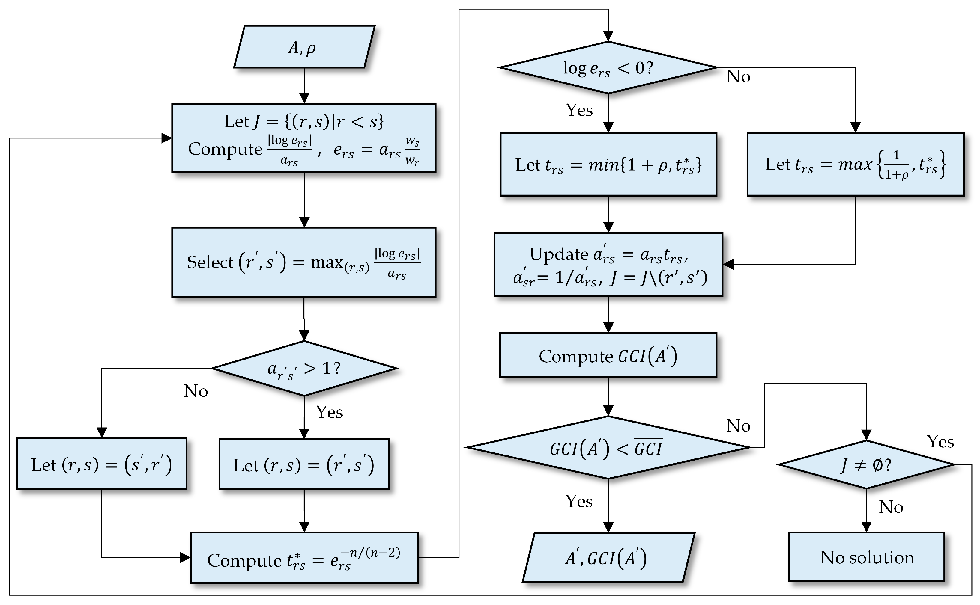
Algorithm 2. GCI-based individual consistency improvement algorithm.

Input: The initial pairwise comparison matrix $A$, the permissibility coefficient $\rho$   Output: The modified pairwise comparison matrix $A^{\prime }$, the improved $GCI\left(A^{\prime }\right)$      Step 0. Let $J=\left\{\left(r,s\right)|r<s\right\}$ be the index set corresponding to the expert judgments.   Step 1. Compute $\frac{\left|\log e_{rs}\right|}{a_{rs}}$ for all $\left(r,s\right)\in J$, where $e_{rs}=a_{rs}\frac{w_s}{w_r}$.   Step 2. Choose the pair $\left(r^{\prime },s^{\prime }\right)\in J$ which $\frac{\left|\log e_{r^{\prime }{s}^{\prime }}\right|}{a_{r^{\prime }{s}^{\prime }}}$ has the largest value.   Step 3. If $a_{r^{\prime }{s}^{\prime }}>1$, then let $\left(r,s\right)=\left(r^{\prime },s^{\prime }\right)$. Otherwise, let $\left(r,s\right)=\left(s^{\prime },r^{\prime }\right)$.   Step 4. Compute $t_{rs}^{*}=e_{rs}^{-n/\left(n-2\right)}$.   Modify $a_{rs}$ with $t_{rs}$, which depends on the sign of $\log e_{rs}$.   a.  If $\log e_{rs}<0$, let $t_{rs}=min\left\{1+\rho ,t_{rs}^{*}\right\}$.   b.  If $\log e_{rs}>0$, let $t_{rs}=max\left\{\frac{1}{1+\rho },t_{rs}^{*}\right\}$.   Update matrix $A$ with revised values $a_{rs}^{\prime }=a_{rs}{t}_{rs}$ and $a_{sr}^{\prime }=1/a_{rs}^{\prime }$.   Update index set $J=J\backslash \left(r^{\prime },s^{\prime }\right)$.   Step 5. Compute $GCI\left(A^{\prime }\right)$.   a.  If $GCI\left(A^{\prime }\right)<\overline{GCI}$, provide $A^{\prime }$ and $GCI\left(A^{\prime }\right)$.   b.  Otherwise, if $J\ne \varnothing$, repeat steps 1 through 4.   c.  Otherwise, the algorithm has no solution, so enlarge the permissibility coefficient $\rho$ or organize experts to modify the judgments.

2.3.3. Expert Preference Aggregation

In expert preference aggregation, the individual authorities and consistency levels impact the aggregation results [80]. Inspired by this, we propose a novel GCI-based operator to integrate the expert weights.

$${\lambda }_k^p=\alpha w_k^p+\beta {\nu }_k^p,$$

(21)

$${\nu }_k^p=\frac{1}{GC{I}_k}/{{\displaystyle \sum }}_{k=1}^l\frac{1}{GC{I}_k},$$

(22)

where ${\nu }_k^p$ represents the weight of individual consistency level, satisfying $0<{\nu }_k^p<1$, and ${{\displaystyle \sum }}_{k=1}^l{\nu }_k^p=1$. It is worth noting that the $GC{I}_k$ here corresponds to the modified individual judgment matrix, not the original individual judgment matrix. The smaller the value of $GC{I}_k$, the larger the value of ${\nu }_k^p$. In addition, $\alpha$ and $\beta$ are the distribution coefficients, satisfying $\alpha +\beta =1$, $\alpha ,\beta \in R^{+}$. They provide substantial flexibility for expert preference aggregation. In particular, when $\alpha =1$ and $\beta =0$, the Hadamard coefficient is equal to the expert authority weight. In contrast, when $\alpha =0$ and $\beta =1$, the Hadamard coefficient is equal to the improved individual consistency level.

The weighted geometric average operator (WGA) is used to aggregate the individual judgment matrices, with the group judgment matrix $B={\left[b_{ij}\right]}_{n\times n}$ developed as

$$b_{ij}={{\displaystyle \prod }}_{k=1}^l{\left(a_{ij}^k\right)}^{{\lambda }_k^p}.$$

(23)

The group judgment matrix aggregated using the WGA operators has the same properties as the positive reciprocal judgment matrices, and its GCI is less than or at most equal to that of the least consistent individual judgment matrix [81,82]. Therefore, provided that the individual judgment matrix has acceptable consistency, the group judgment matrix aggregated using the WGA operators must be acceptable.

$$GCI\left(B\right)\le max\left\{GCI\left(A_1\right),GCI\left(A_2\right),\dots ,GCI\left(A_l\right)\right\}.$$

(24)

2.3.4. Group Consensus Verification

The group cardinal consensus index (GCCI) of individual judgment matrices [83] can be calculated as follows

$$GCCI\left(A_k\right)=1-\frac{1}{\left(n-1\right)\left(n-2\right)ln9}{{\displaystyle \sum }}_{i=1}^{n-1}{{\displaystyle \sum }}_{j=i+1}^n\left|ln\left(b_{ij}\right)-ln\left(a_{ij}^k\right)\right|,$$

(25)

and the overall group consensus index is given by:

$$GCCI\left(B\right)={{\displaystyle \sum }}_{k=1}^l{\lambda }_k^p·GCCI\left(A_k\right).$$

(26)

The larger the values of $GCCI\left(A_k\right)$, the higher the consensus levels between the group judgment matrix $B$ and the individual judgment matrix $A_k$, i.e., the higher the recognition of the aggregation results by the expert $P_k$. Let $\overline{GCCI}$ be the predetermined threshold; if $GCCI\left(A_k\right)\ge \overline{GCCI}$, then the aggregated group judgment matrix $B$ has an acceptable cardinal consensus with the individual judgment matrix $A_k$, and if $GCCI\left(A_k\right)\ge \overline{GCCI}$ for all individual judgment matrices, acceptable group consensus is achieved by the expert group. The value of $\overline{GCCI}$ can be subjectively determined by the expert group or a highly experienced expert [83].

Some previously proposed indices [58,65] are listed as follows for measuring the degree to which the original expert preference information is preserved.

• Geometric Compatibility Index (GCOMPI): the cardinal compatibility between the group priority vector and the individual expert judgments.

  $$GCOMPI\left(B\right)={{\displaystyle \sum }}_{k=1}^l{\lambda }_k^p·GCOMPI\left(A_k\right),$$

  (27)

  $$GCOMPI\left(A_k\right)=\frac{2}{\left(n-1\right)\left(n-2\right)}{{\displaystyle \sum }}_{i<j}lo{g}^2\left(a_{ij}^k{w}_j/w_i\right),$$

  (28)

  where $w={\left(w_i\right)}_{n\times 1}$ is the priority vector derived from the group judgment matrix $B$.
• Priority violation number for the expert group (PVN): the ordinal compatibility between the group priority vector and the individual expert judgments.

  $$PVN\left(B\right)={{\displaystyle \sum }}_{k=1}^l{\lambda }_k^p·PVN\left(A_k\right),$$

  (29)

  $$PVN\left(A_k\right)=\frac{2}{\left(n-1\right)\left(n-2\right)}{{\displaystyle \sum }}_{i<j}{I}_{ij}\left(A_k/B\right),$$

  (30)

  $$I_{ij}\left(A_k/B\right)=\{\begin{array}{cc}1& if a_{ij}^k>1 and w_i<w_j\\ 1& if a_{ij}^k<1 and w_i>w_j\\ 0.5& if a_{ij}^k=1 and w_i\ne w_j\\ 0.5& if a_{ij}^k\ne 1 and w_i=w_j\\ 0& otherwise\end{array},$$

  (31)

  where $w={\left(w_i\right)}_{n\times 1}$ is the priority vector derived from the group judgment matrix $B$.
• Average variance (AV): the average change between the group priority vector and the individual priority vector.

  $$d\left(w,w^k\right)=\frac{1}{n}{{\displaystyle \sum }}_{i=1}^n\left|w_i-w_i^k\right|,$$

  (32)

  where $w={\left(w_i\right)}_{n\times 1}$ is the priority vector derived from the group judgment matrix $B$ and $w^k={\left(w_i^k\right)}_{n\times 1}$ is the priority vector derived from the individual judgment matrix $A_k$.
• Kendall’s tau distance ($\tau$): the ranking changes between two rankings derived from the group judgment matrix $B$ and the individual judgment matrix $A_k$.

  $$\tau \left({\gamma }_B,{\gamma }_{A_k}\right)=\frac{2}{n\left(n-1\right)}\left(N_{concordant pairs}-N_{disconcordant pairs}\right),$$

  (33)

  where ${\gamma }_B$ and ${\gamma }_{A_k}$ are the two rankings (permutations) of $n$ indicators, and $N_{concordantpairs}$ and $N_{disconcordantpairs}$ are the numbers of concordant pairs and disconcordant pairs, respectively, between the two rankings. Therefore, $-1\le \tau \left({\gamma }_B,{\gamma }_{A_k}\right)\le 1$, with larger values of $\tau \left({\gamma }_B,{\gamma }_{A_k}\right)$ corresponding to higher ordinal consensus levels between the group judgment matrix $B$ and the individual judgment matrix $A_k$.

2.4. Fuzzy TOPSIS Technique to Evaluate, Rank and Select Ship Designs

This section presents an applicable Fuzzy TOPSIS method to evaluate, rank and select alternative ship designs regarding ship-equipment suitability. TOPSIS [84] is one of the classical MCDM methods; Fuzzy TOPSIS is its further development under fuzzy set theory [85]. The theoretical background of fuzzy sets can be reviewed in [19,85,86].

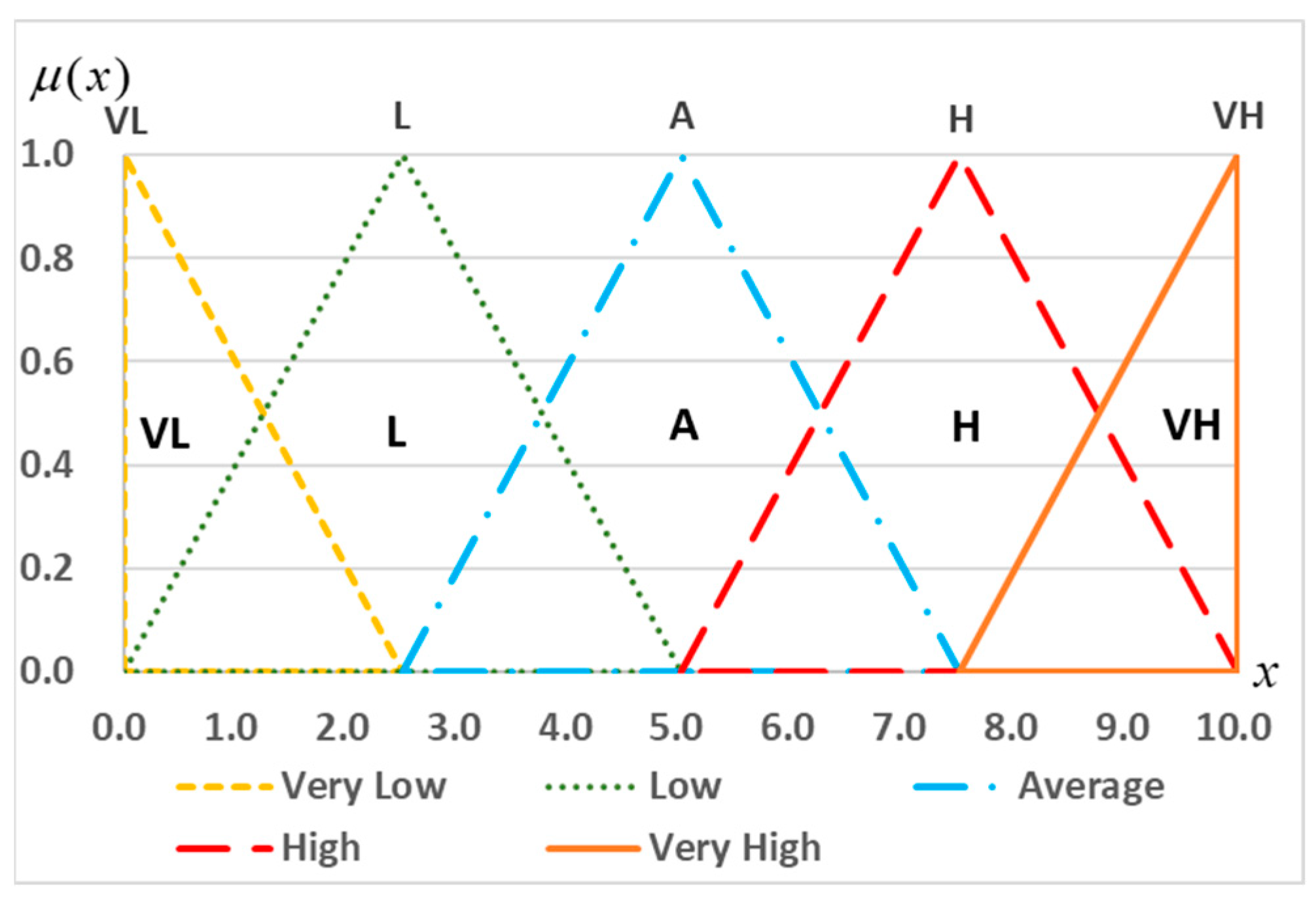
2.4.1. Linguistic Scales

Miller [87] demonstrated that an individual could not simultaneously compare more than 7 ± 2 objects without confusion. Therefore, to reduce the mental workload of experts, five-level linguistic scales, i.e., VL-L-A-H-VH, are designed as a fuzzy cluster to evaluate the criteria performances (score values) of alternative ship-equipment suitability designs and to help experts to make their subjective decisions. For example, suppose one expert gives a linguistic evaluation A on one criterion performance for one ship design. In that case, the pertinence degree of the score values from 2.5 to 7.5 ranges from 0.0 to 1.0, with the largest pertinence degree of 1.0 at the score value of 5.0 and the lowest pertinence degree of 0.0 at the score values of 2.5 and 7.5, as shown in the blue triangle in Figure 7. The mapping relationships between the linguistic scales and triangular fuzzy numbers (TFNs) [19] are shown in

Table 4. Linguistic terms and corresponding TFNs.

Linguistic Terms (Evaluation Set)	TFNs
Very low (VL)	(0.0, 0.0, 2.5)
Low (L)	(0.0, 2.5, 5.0)
Average (A)	(2.5, 5.0, 7.5)
High (H)	(5.0, 7.5, 10.0)
Very high (VH)	(7.5, 10.0, 10.0)

and Figure 7.

2.4.2. Fuzzy TOPSIS Technique

Let $F=\left\{f_1,f_2,\dots ,f_m\right\}$ be the alternative designs, $C=\left\{c_1,c_2,\dots ,c_n\right\}$ be the assessment indicators, and $W^C={\left(w_1^c,w_2^c,\dots ,w_n^c\right)}^T$ be the weight vector for assessment indicators. We have $0<w_j^c<1$, and ${{\displaystyle \sum }}_{j=1}^n{w}_j^c=1$. As such, the Fuzzy TOPSIS method comprises the following steps.

Step 1: Develop the individual fuzzy decision matrix ${\tilde{D}}_k$:

$$\begin{array}{c}\\ {\tilde{D}}_k=\end{array}\begin{array}{cc}& \begin{array}{cc}\begin{array}{cc}{C}_1& C_2\end{array}& \begin{array}{cc}{C}_j& C_n\end{array}\end{array}\\ \begin{array}{c}\begin{array}{c}{F}_1\\ F_2\end{array}\\ \begin{array}{c}{F}_i\\ F_m\end{array}\end{array}& \left[\begin{array}{cc}\begin{array}{cc}{\tilde{x}}_{11}^k& {\tilde{x}}_{12}^k\\ {\tilde{x}}_{21}^k& {\tilde{x}}_{22}^k\end{array}& \begin{array}{cc}\cdots & {\tilde{x}}_{1n}^k\\ \cdots & {\tilde{x}}_{2n}^k\end{array}\\ \begin{array}{cc}⋮& ⋮\\ {\tilde{x}}_{m1}^k& {\tilde{x}}_{m2}^k\end{array}& \begin{array}{cc}\ddots & ⋮\\ \cdots & {\tilde{x}}_{mn}^k\end{array}\end{array}\right]\end{array},$$

(34)

where ${\tilde{x}}_{ij}^k$ denotes the rating of the $i$th alternative $F_i$, concerning the $j$th criterion $C_j$, given by the $k$th expert $P_k$.

Step 2: Aggregate the ratings of alternative designs provided by the experts using Equation (35) and develop the fuzzy decision matrix $\tilde{D}$ using Equation (36):

$${\tilde{x}}_{ij}={{\displaystyle \sum }}_{k=1}^l{w}_k^p·{\tilde{x}}_{ij}^k,$$

(35)

$$\begin{array}{c}\\ \tilde{D}=\end{array}\begin{array}{cc}& \begin{array}{cc}\begin{array}{cc}{C}_1& C_2\end{array}& \begin{array}{cc}{C}_j& C_n\end{array}\end{array}\\ \begin{array}{c}\begin{array}{c}{F}_1\\ F_2\end{array}\\ \begin{array}{c}{F}_i\\ F_m\end{array}\end{array}& \left[\begin{array}{cc}\begin{array}{cc}{\tilde{x}}_{11}& {\tilde{x}}_{12}\\ {\tilde{x}}_{21}& {\tilde{x}}_{22}\end{array}& \begin{array}{cc}\cdots & {\tilde{x}}_{1n}\\ \cdots & {\tilde{x}}_{2n}\end{array}\\ \begin{array}{cc}⋮& ⋮\\ {\tilde{x}}_{m1}& {\tilde{x}}_{m2}\end{array}& \begin{array}{cc}\ddots & ⋮\\ \cdots & {\tilde{x}}_{mn}\end{array}\end{array}\right]\end{array}.$$

(36)

Step 3: Normalize the fuzzy decision matrix $\tilde{D}$ using Equations (37) and (38). Then, the normalized fuzzy decision matrix $\tilde{R}={\left[{\tilde{r}}_{ij}\right]}_{n\times n}$ is constructed as follows:

Benefit criteria:

$${\tilde{r}}_{ij}=\left(\frac{l_{ij}}{u_j^{+}},\frac{m_{ij}}{u_j^{+}},\frac{u_{ij}}{u_j^{+}}\right),u_j^{+}=\underset{i}{\max }{u}_{ij},$$

(37)

Cost criteria:

$${\tilde{r}}_{ij}=\left(\frac{l_j^{-}}{u_{ij}},\frac{l_j^{-}}{m_{ij}},\frac{l_j^{-}}{l_{ij}}\right),l_j^{-}=\underset{i}{\min }{l}_{ij}.$$

(38)

Step 4: Compute the weighted normalised decision matrix $\tilde{V}={\left[{\tilde{\nu }}_{ij}\right]}_{n\times n}$:

$${\tilde{\nu }}_{ij}=w_j^c·{\tilde{r}}_{ij}.$$

(39)

Step 5: Define the Fuzzy Positive Ideal Solution (FPIS, $F^{+}$) and Fuzzy Negative Ideal Solution (FNIS, $F^{-}$) according to Equations (40) and (41), respectively:

$$F^{+}=\left({\tilde{\nu }}_1^{+},{\tilde{\nu }}_2^{+},{\tilde{\nu }}_j^{+},\dots ,{\tilde{\nu }}_n^{+}\right)$$

(40)

$$F^{-}=\left({\tilde{\nu }}_1^{-},{\tilde{\nu }}_2^{-},{\tilde{\nu }}_3^{-},\dots ,{\tilde{\nu }}_n^{-}\right),$$

(41)

where ${\tilde{\nu }}_j^{+}=\left(1,1,1\right)$ and ${\tilde{\nu }}_j^{-}=\left(0,0,0\right)$.

Step 6: Compute the distances $d_i^{+}$ and $d_i^{-}$ of each alternative from ${\tilde{\nu }}_j^{+}$ and ${\tilde{\nu }}_j^{-}$, respectively, according to Equations (42) and (43):

$$d_i^{+}={{\displaystyle \sum }}_{j=1}^n{d}_{\nu }\left({\tilde{\nu }}_{ij},{\tilde{\nu }}_j^{+}\right),$$

(42)

$$d_i^{-}={{\displaystyle \sum }}_{j=1}^n{d}_{\nu }\left({\tilde{\nu }}_{ij},{\tilde{\nu }}_j^{-}\right),$$

(43)

where $d_{\nu }(\cdots )$ is the distance between fuzzy numbers. For TFNs, $d_{\nu }(\cdots )$ is expressed as

$$d\left(\tilde{x},\tilde{z}\right)=\sqrt{\frac{1}{3}\left[{\left(l_x-l_z\right)}^2+{\left(m_x-m_z\right)}^2+{\left(u_x-u_z\right)}^2\right]}.$$

(44)

Step 7: Compute the closeness coefficient $C{C}_i$:

$$C{C}_i=\frac{d_i^{-}}{d_i^{+}+d_i^{-}}.$$

(45)

Step 8: Define the rankings of alternatives according to the closeness coefficient $C{C}_i$ in decreasing order. The best alternative is closest to the FPIS and farthest to the FNIS.

3. Case Study: Ship-Equipment Environmental Suitability Evaluation

This section applies the proposed framework to evaluate, rank, and select alternative ship designs regarding ship-equipment environmental suitability.

3.1. Problem Statement

Ship-equipment environmental suitability refers to the capability of motherships and shipborne equipment to cooperatively complete operational missions under physical, chemical, biological, and other environmental conditions. It is one of the most challenging design tasks faced by ship designers since it is critical to the operational security and efficiency of motherships and shipborne equipment. In practical design tasks, ship designers fully consider the material of parent ships, their knowledge and experience, and other available design means, as well as the relevant design constraints, to generate several initial design solutions that satisfy the given operational performance requirements, such as the capability of launching and recovery of amphibious vehicles. The criteria performances of these design solutions may be varied, which makes it necessary to develop a scientific evaluation system to assess these criteria performances thoroughly. Scientifically evaluating alternative ship designs can help identify their strengths and weaknesses and provide ship designers with decision guidance and optimization bases to facilitate improved ship designs. In this context, this paper presents an MCDM framework to guide the decision-makers in evaluating alternative ship designs regarding ship-equipment environmental suitability.

3.2. Establishment of the Expert Group

The inherent complexity of amphibious warships has brought great difficulty to the scientific evaluation of ship-equipment environmental suitability. Empirical assessments based on expert knowledge can be acceptable solutions in this case. In this investigation, three experienced experts were invited to construct the evaluation index systems, distribute the index weights, and evaluate and compare the criteria performances of several ship-equipment suitability environmental designs. The expert profile details are provided in

Table 5. Expert profile details.

Expert	Institute	Job Title	Educational Level	Years Experienced	Age
$P_1$	MARIC a	Chief Engineer, Prof.	Ph.D.	18	46
$P_2$	HEU b	Prof.	Ph.D.	12	41
$P_3$	SMERI c	Chief Engineer, Prof.	Ph.D.	15	43

^a MARIC: Marine Design & Research Institute of China; ^b HEU: Harbin Engineering University; ^c SMERI: Shanghai Marine Equipment Research Institute.

.

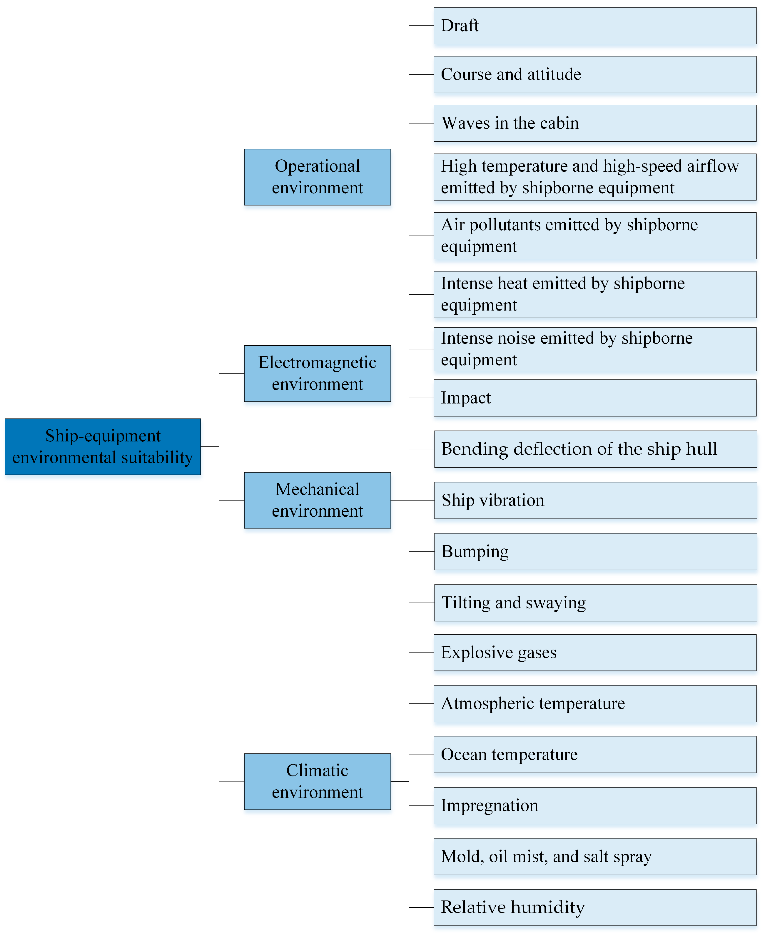
3.3. Identification and Selection of Assessment Indicators

This investigation utilized the improved ISM method to construct the ship-equipment environmental suitability evaluation index system. This process involved semi-structured interviews with the three experienced experts to identify and select the appropriate assessment indicators. The final list of detailed indicators is furnished in

Table 6. Ship-equipment environmental suitability assessment indicators.

No.	Indicators	Description	Unit	Benefit/Cost
$X_1$	Explosive gases	The explosion-proof electrical equipment and prevention measures in explosive dangerous places where explosive gases accumulate or spread must satisfy the safety requirements.	Linguistic	Benefit
$X_2$	Operational environment	The actual environmental conditions under the coupling of various factors should satisfy the environmental requirements for the normal operation of the mothership, shipborne equipment, and ship crew.	Linguistic	Benefit
$X_3$	Impact	The anti-impact design of ship hull and shipborne equipment should be carried out to enable them to operate safely in cases of severe impacts such as underwater explosions.	Linguistic	Benefit
$X_4$	Bending deflection of the ship hull	The maximum bending deflection of the ship hull with the wave and still bending moment coupling should be less than a critical value.	m	Cost
$X_5$	Ship vibration	The ship hull’s natural frequency must avoid the propellers’ and generators’ operating frequency. The vibration amplitude of the ship hull must also be controlled.	%	Benefit
$X_6$	Atmospheric temperature	The normal working and non-damage temperatures of shipborne equipment should be adapted to the ambient atmospheric temperature.	°C	Benefit
$X_7$	Bumping	Shipborne equipment should withstand repetitive low-intensity bumping caused by wave shocks (including bow shocks, stern shocks, etc.) and operate continuously and effectively.	Linguistic	Benefit
$X_8$	Electromagnetic environment	The spectrum allocation of electronic equipment should be compatible with the management and control measures in time, space, frequency domain, and power supply.	Linguistic	Benefit
$X_9$	Oceanic temperature	The normal working and non-damage temperatures of shipborne equipment exposed to seawater should be adapted to the ocean temperature.	°C	Benefit
$X_{10}$	Mechanical environment	A general term for environmental factors, such as tilting, swaying, vibration, and impact caused by the navigation attitude of the mothership, the running state of shipborne equipment, and other influencing factors.	Linguistic	Benefit
$X_{11}$	Impregnation	The effects of impregnation on shipborne equipment should be considered, and waterproof or watertight design should be carried out for specific shipborne equipment.	Linguistic	Benefit
$X_{12}$	Mold, oil mist, and salt spray	The effects of mold, oil mist, and salt spray on shipborne equipment should be considered. The climate protection design should be carried out so that the shipborne equipment can operate normally under specific molds, oil mist, and salt spray concentrations.	Linguistic	Benefit
$X_{13}$	Draft	The mothership should be able to sink to appropriate draught at a certain speed so that the shipborne equipment can smoothly get in and out of the cabin.	Linguistic	Benefit
$X_{14}$	Course and attitude	The mothership should control its course and attitude so the shipborne equipment can smoothly get in and out of the cabin.	Linguistic	Benefit
$X_{15}$	Climatic environment	The climatic factors that have an impact on the mothership and shipborne equipment.	Linguistic	Benefit
$X_{16}$	Tilting and swaying	The mothership should adequately control the amplitude and period of its tilting and swaying so that the coverage area of the envelope diagram describing the normal operation of shipborne equipment is at least a specific value.	%	Benefit
$X_{17}$	Relative humidity	Shipborne equipment should operate normally in a specific range of relative humidity.	%	Benefit
$X_{18}$	Waves in the cabin	The mother ship should control its course and attitude and install wave suppression devices so the shipborne equipment can smoothly get in and out of the cabin.	Linguistic	Benefit
$X_{19}$	High temperature and high-speed airflow emitted by shipborne equipment	To deal with the high-temperature and high-speed airflow emitted by shipborne equipment, protective designs, and prevention measures should be carried out to enable the mothership, shipborne equipment, and ship crew to operate safely.	Linguistic	Benefit
$X_{20}$	Air pollutants emitted by shipborne equipment	To deal with the air pollutants emitted by shipborne equipment, protective designs, and prevention measures should be carried out to enable the shipborne equipment and ship crew to operate safely.	Linguistic	Benefit
$X_{21}$	Intense heat emitted by shipborne equipment	Protective designs and prevention measures should be carried out to deal with the intense heat emitted by shipborne equipment to enable the mothership, shipborne equipment, and ship crew to operate safely.	Linguistic	Benefit
$X_{22}$	Intense noise emitted by shipborne equipment	Protective designs and prevention measures should be carried out to deal with the intense noise emitted by shipborne equipment to enable the mothership, shipborne equipment, and ship crew to operate safely.	Linguistic	Benefit

, along with the pertinent descriptions.

3.4. Construction of Appropriate Hierarchical Structures

To reduce the subjective arbitrariness, pairwise comparison judgments were applied to analyze the interrelations among the assessment indicators, with SSIMs $O_k$ developed using Equation (1).

$O_1$

1

2

3

4

5

6

7

8

9

10

11

12

13

14

15

16

17

18

19

20

21

22

1

~

>

×

×

×

×

×

×

×

×

×

×

×

×

>

×

×

×

×

×

×

×

2

~

×

×

×

×

×

×

×

×

×

×

<

<

×

×

×

<

<

<

<

<

3

~

×

×

×

×

×

×

>

×

×

×

×

×

×

×

×

×

×

×

×

4

~

×

×

×

×

×

>

×

×

×

×

×

×

×

×

×

×

×

×

5

~

×

×

×

×

>

×

×

×

×

×

×

×

×

×

×

×

×

6

~

×

×

×

×

×

×

×

×

>

×

×

×

×

×

×

×

7

~

×

×

>

×

×

×

×

×

×

×

×

×

×

×

×

8

~

×

×

×

×

×

×

×

×

×

×

×

×

×

×

9

~

×

×

×

×

×

>

×

×

×

×

×

×

×

10

~

×

×

×

×

×

<

×

×

×

×

×

×

11

~

×

×

×

>

×

×

×

×

×

×

×

12

~

×

×

>

×

×

×

×

<

×

×

13

~

×

×

×

×

×

×

×

×

×

14

~

×

×

×

×

×

×

×

×

15

~

×

<

×

×

×

×

×

16

~

×

×

×

×

×

×

17

~

×

×

×

×

×

18

~

×

×

×

×

19

~

×

×

×

20

~

×

×

21

~

×

22

~

$O_2$

1

2

3

4

5

6

7

8

9

10

11

12

13

14

15

16

17

18

19

20

21

22

1

~

×

×

×

×

×

×

×

×

×

×

×

×

×

>

×

×

×

×

×

×

×

2

~

×

×

<

<

<

×

<

×

×

×

×

<

×

<

<

<

<

<

<

<

3

~

×

×

×

×

×

×

>

×

×

×

×

×

×

×

×

×

×

×

×

4

~

×

×

×

×

×

>

×

×

×

×

×

×

×

×

×

×

×

×

5

~

×

×

×

×

>

×

×

×

×

×

×

×

×

×

×

×

×

6

~

×

×

×

×

×

×

×

×

>

×

×

×

×

×

×

×

7

~

×

×

>

×

×

×

×

×

×

×

×

×

×

×

×

8

~

×

×

×

×

×

×

×

×

×

×

×

×

×

×

9

~

×

×

×

×

×

>

×

×

×

×

×

×

×

10

~

×

×

×

×

×

<

×

×

×

×

×

×

11

~

×

×

×

>

×

<

×

×

×

×

×

12

~

×

×

>

×

<

×

×

×

×

×

13

~

>

×

×

×

×

×

×

×

×

14

~

×

<

×

>

×

×

×

×

15

~

×

<

×

×

×

×

×

16

~

×

>

×

×

×

×

17

~

×

×

×

×

×

18

~

×

×

×

×

19

~

×

×

×

20

~

×

×

21

~

×

22

~

$O_3$

1

2

3

4

5

6

7

8

9

10

11

12

13

14

15

16

17

18

19

20

21

22

1

~

×

×

×

×

×

×

×

×

×

×

×

×

×

>

×

×

×

×

×

×

×

2

~

×

×

×

×

×

×

×

×

×

×

<

<

×

×

×

<

<

<

<

<

3

~

>

×

×

×

×

×

>

×

×

×

×

×

×

×

×

×

×

×

×

4

~

×

×

<

×

×

>

×

×

×

×

×

×

×

×

×

×

×

×

5

~

×

×

×

×

>

×

×

×

×

×

×

×

×

×

×

×

×

6

~

×

×

×

×

×

×

×

×

>

×

×

×

×

×

×

×

7

~

×

×

>

×

×

×

×

×

×

×

×

×

×

×

×

8

~

×

×

×

×

×

×

×

×

×

×

×

×

×

×

9

~

×

×

×

×

×

>

×

×

×

×

×

×

×

10

~

<

<

×

×

×

<

<

×

×

×

<

×

11

~

×

×

×

>

×

×

×

×

×

×

×

12

~

×

×

>

×

×

×

×

×

×

×

13

~

×

×

×

×

×

×

×

×

×

14

~

×

×

×

×

×

×

×

×

15

~

×

<

×

×

×

×

×

16

~

×

×

×

×

×

×

17

~

×

×

×

×

×

18

~

×

×

×

×

19

~

×

×

×

20

~

×

×

21

~

×

22

~

The SSIMs $O_k$ were converted to the IRMs $A_k$ using Equation (2), then the IRMs $A_k$ were further transformed into the FRMs $R_k$ using Equation (3). The expert authority weights were set to $W^P={\left(0.4,0.3,0.3\right)}^T$ and the individual judgments were counted using Equations (7) and (8). The threshold for aggregating the expert judgments was set to $t=0.5$, provided that expert $P_1$ and either $P_2$ or $P_3$ or both agreed that $X_i$ affects $X_j$, the expert group was considering agreeing that $X_i$ affects $X_j$. The expert judgments were further aggregated, with the group reachability matrix $B$ developed using Equation (9). The transitivity among the assessment indicators was eliminated using Equations (5) and (6), and the FRMs $R_k$ and the group reachability matrix $B$ was transformed into the skeleton matrices $S_k$ and $S_B$.

It is believed that the thresholds of 0.9 have high engineering credibility, so the thresholds $\overline{CCG}$ and $\overline{DVN}$ were set to $\overline{CCG}=\overline{DVN}=0.9$. The group consensus indices CCG and DVN were calculated using Equations (10)–(16) (see

Table 7. Results of group consensus indices.

Expert	$\mathit{C}\mathit{C}{\mathit{G}}_{0.9}$	$\mathit{D}\mathit{V}{\mathit{N}}_{0.9}$
$P_1$	0.9710	0.9957
$P_2$	0.8489 0.9037	0.9719 0.9805
$P_3$	0.9106	0.9827
Group	0.9162 0.9327	0.9846 0.9872

). It is seen from Table 7 that expert $P_2$ failed the group consensus verification, and consequently, the individual skeleton matrix $S_2$ was modified using the group consensus improvement algorithm. The revised group consensus indices can be found in Table 7 (bold, italic), with the results indicating that by slightly modifying individual expert judgments, the expert group achieved acceptable group consensus.

The assessment indicators were divided into several irrelevant or rarely relevant subsets using Equation (4), as shown in

Table 8. Division of the assessment indicators.

Subsets	Indicators
1	2, 13, 14, 18, 19, 20, 21, 22
2	8
3	3, 4, 5, 7, 10, 16
4	1, 6, 9, 11, 12, 15, 17

. On this basis, the divided subsets of the assessment indicators were further partitioned into several levels using Equation (4), as shown in

Table 9. Level partition of the assessment indicators.

Hierarchical Levels	Indicators
1	2, 8, 10, 15
2	1, 3, 4, 5, 6, 7, 9, 11, 12, 13, 14, 16, 17, 18, 19, 20, 21, 22

.

Finally, the hierarchical structure of the assessment indicators was developed according to the divided subsets, partitioned levels, and converted skeleton matrices. The overall index system for evaluating ship-equipment environmental suitability based on the improved ISM method is shown in Figure 8.

3.5. Weight Distribution for the Assessment Indicators

This investigation utilized the improved AHP method to distribute appropriate weights for ship-equipment environmental suitability assessment indicators. Owing to space limitations, only the detailed process and results for the typical weighting node 2 (operational environment) are presented as follows.

The initial individual judgment matrices $A_2^k$ were developed using Equation (17) as follows.

$$\begin{gathered} A_2^1=\begin{array}{cc}\begin{array}{c}\begin{array}{c}{X}_{13}\\ X_{14}\end{array}\\ \begin{array}{c}{X}_{18}\\ X_{19}\end{array}\\ \begin{array}{c}{X}_{20}\\ \begin{array}{c}{X}_{21}\\ X_{22}\end{array}\end{array}\end{array}& \left[\begin{array}{ccc}\begin{array}{c}\begin{array}{c}\begin{array}{c}1\\ \\ \end{array}\\ \\ \end{array}\\ \\ \end{array}& \begin{array}{c}\begin{array}{c}\begin{array}{c}3\\ 1\\ \end{array}\\ \\ \end{array}\\ \\ \end{array}& \begin{array}{ccc}\begin{array}{c}\begin{array}{c}\begin{array}{c}5\\ 5\\ 1\end{array}\\ \\ \end{array}\\ \\ \end{array}& \begin{array}{c}\begin{array}{c}\begin{array}{c}7\\ 5\\ 3\end{array}\\ 1\\ \end{array}\\ \\ \end{array}& \begin{array}{ccc}\begin{array}{c}\begin{array}{c}\begin{array}{c}9\\ 7\\ 5\end{array}\\ 5\\ 1\end{array}\\ \\ \end{array}& \begin{array}{c}\begin{array}{c}\begin{array}{c}7\\ 7\\ 5\end{array}\\ 5\\ 1/3\end{array}\\ 1\\ \end{array}& \begin{array}{c}\begin{array}{c}\begin{array}{c}9\\ 7\\ 5\end{array}\\ 5\\ 1\end{array}\\ 2\\ 1\end{array}\end{array}\end{array}\end{array}\right]\end{array},A_2^2=\begin{array}{cc}\begin{array}{c}\begin{array}{c}{X}_{13}\\ X_{14}\end{array}\\ \begin{array}{c}{X}_{18}\\ X_{19}\end{array}\\ \begin{array}{c}{X}_{20}\\ \begin{array}{c}{X}_{21}\\ X_{22}\end{array}\end{array}\end{array}& \left[\begin{array}{ccc}\begin{array}{c}\begin{array}{c}\begin{array}{c}1\\ \\ \end{array}\\ \\ \end{array}\\ \\ \end{array}& \begin{array}{c}\begin{array}{c}\begin{array}{c}3\\ 1\\ \end{array}\\ \\ \end{array}\\ \\ \end{array}& \begin{array}{ccc}\begin{array}{c}\begin{array}{c}\begin{array}{c}5\\ 3\\ 1\end{array}\\ \\ \end{array}\\ \\ \end{array}& \begin{array}{c}\begin{array}{c}\begin{array}{c}5\\ 5\\ 3\end{array}\\ 1\\ \end{array}\\ \\ \end{array}& \begin{array}{ccc}\begin{array}{c}\begin{array}{c}\begin{array}{c}7\\ 5\\ 3\end{array}\\ 3\\ 1\end{array}\\ \\ \end{array}& \begin{array}{c}\begin{array}{c}\begin{array}{c}7\\ 5\\ 3\end{array}\\ 3\\ 1/2\end{array}\\ 1\\ \end{array}& \begin{array}{c}\begin{array}{c}\begin{array}{c}7\\ 6\\ 3\end{array}\\ 5\\ 1\end{array}\\ 1\\ 1\end{array}\end{array}\end{array}\end{array}\right],\end{array} \\ {A}_2^3=\begin{array}{cc}\begin{array}{c}\begin{array}{c}{X}_{13}\\ X_{14}\end{array}\\ \begin{array}{c}{X}_{18}\\ X_{19}\end{array}\\ \begin{array}{c}{X}_{20}\\ \begin{array}{c}{X}_{21}\\ X_{22}\end{array}\end{array}\end{array}& \left[\begin{array}{ccc}\begin{array}{c}\begin{array}{c}\begin{array}{c}1\\ \\ \end{array}\\ \\ \end{array}\\ \\ \end{array}& \begin{array}{c}\begin{array}{c}\begin{array}{c}3\\ 1\\ \end{array}\\ \\ \end{array}\\ \\ \end{array}& \begin{array}{ccc}\begin{array}{c}\begin{array}{c}\begin{array}{c}5\\ 7\\ 1\end{array}\\ \\ \end{array}\\ \\ \end{array}& \begin{array}{c}\begin{array}{c}\begin{array}{c}7\\ 7\\ 3\end{array}\\ 1\\ \end{array}\\ \\ \end{array}& \begin{array}{ccc}\begin{array}{c}\begin{array}{c}\begin{array}{c}9\\ 9\\ 5\end{array}\\ 5\\ 1\end{array}\\ \\ \end{array}& \begin{array}{c}\begin{array}{c}\begin{array}{c}9\\ 9\\ 5\end{array}\\ 5\\ 1/2\end{array}\\ 1\\ \end{array}& \begin{array}{c}\begin{array}{c}\begin{array}{c}9\\ 9\\ 5\end{array}\\ 5\\ 1\end{array}\\ 3\\ 1\end{array}\end{array}\end{array}\end{array}\right]\end{array} \end{gathered}$$

The index weights for each expert were calculated using Equations (18) and (19). Then, the individual consistency indices $GC{I}_k$ were calculated using Equation (20). The calculated results are presented in

Table 10. Individual weighting results for Node 2.

Expert	${\mathit{X}}_{13}$	${\mathit{X}}_{14}$	${\mathit{X}}_{18}$	${\mathit{X}}_{19}$	${\mathit{X}}_{20}$	${\mathit{X}}_{21}$	${\mathit{X}}_{22}$	$\mathit{G}\mathit{C}{\mathit{I}}_{0.37}$
$P_1$	0.4180	0.2709	0.1280	0.0891	0.0259	0.0406	0.0275	0.3399
$P_2$	0.4132	0.2494	0.1232	0.0900	0.0386	0.0470	0.0386	0.2189
$P_3$	0.4092	0.3094	0.1168	0.0802	0.0251	0.0357	0.0236	0.3709 0.3593

. It is seen from Table 10 that expert $P_3$ failed the individual consistency verification ($GC{I}_3>0.37$). The individual judgment matrix $A_2^3$ was then modified using the individual consistency improvement algorithm with the permissibility coefficient set to $\rho =0.1$, resulting in the revised individual judgment matrix ${A_2^3}^{\prime }$ given as follows. The revised individual consistency index $GCI\left({A_2^3}^{\prime }\right)$ can be found in Table 10 (bold, italic), with the results indicating that by slightly modifying individual expert judgments, expert $P_3$ achieved acceptable individual consistency.

$${A_2^3}^{\prime }=\begin{array}{cc}\begin{array}{c}\begin{array}{c}{X}_{13}\\ X_{14}\end{array}\\ \begin{array}{c}{X}_{18}\\ X_{19}\end{array}\\ \begin{array}{c}{X}_{20}\\ \begin{array}{c}{X}_{21}\\ X_{22}\end{array}\end{array}\end{array}& \left[\begin{array}{ccc}\begin{array}{c}\begin{array}{c}\begin{array}{c}1\\ \\ \end{array}\\ \\ \end{array}\\ \\ \end{array}& \begin{array}{c}\begin{array}{c}\begin{array}{c}3\\ 1\\ \end{array}\\ \\ \end{array}\\ \\ \end{array}& \begin{array}{ccc}\begin{array}{c}\begin{array}{c}\begin{array}{c}5\\ \mathbf{6.3636}\\ 1\end{array}\\ \\ \end{array}\\ \\ \end{array}& \begin{array}{c}\begin{array}{c}\begin{array}{c}7\\ 7\\ 3\end{array}\\ 1\\ \end{array}\\ \\ \end{array}& \begin{array}{ccc}\begin{array}{c}\begin{array}{c}\begin{array}{c}9\\ 9\\ 5\end{array}\\ 5\\ 1\end{array}\\ \\ \end{array}& \begin{array}{c}\begin{array}{c}\begin{array}{c}9\\ 9\\ 5\end{array}\\ 5\\ 0.5\end{array}\\ 1\\ \end{array}& \begin{array}{c}\begin{array}{c}\begin{array}{c}9\\ 9\\ 5\end{array}\\ 5\\ 1\end{array}\\ 3\\ 1\end{array}\end{array}\end{array}\end{array}\right]\end{array}$$

After the individual consistency of each expert was verified, the weights of the individual consistency level ${\nu }_k^p$ and the integrated expert weights ${\lambda }_k^p$ were calculated using Equations (21) and (22), with the distribution coefficients set to $\alpha =\beta =0.5$. The calculated results are also presented in

Table 11. Group consensus in Node 2.

Expert	$\mathit{G}\mathit{C}{\mathit{I}}_{0.37}$	${\mathit{\nu }}_{\mathit{k}}^{\mathit{p}}$	${\mathit{w}}_{\mathit{k}}^{\mathit{p}}$	${\mathit{\lambda }}_{\mathit{k}}^{\mathit{p}}$	$\mathit{G}\mathit{C}\mathit{C}{\mathit{I}}_{0.9}$	GCOMPI	PVN	AV	$\mathit{\tau }$
$P_1$	0.3399	0.2858	0.4	0.3429	0.9684	0.3513	0.0333	0.0028	1.0000
$P_2$	0.2189	0.4438	0.3	0.3719	0.9376	0.2695	0.0667	0.0074	0.9048
$P_3$	0.3593	0.2704	0.3	0.2852	0.9457	0.3988	0.0333	0.0102	0.9048
Group	-	-	-	-	0.9505	0.3344	0.0457	0.0066	0.9374

. The individual judgment matrices $A_2^k$ were aggregated using Equation (23). Then, the index weights of the group judgment matrix $B_2$ were calculated using Equations (18) and (19), with the weighting results as 0.4148, 0.2736, 0.1233, 0.087, 0.0299, 0.0415, and 0.03, respectively. Next, the group consensus indices (GCCI, GCOMPI, PVN, AV, $\tau$) were calculated using Equations (25)–(33) (see Table 11). The threshold $\overline{GCCI}$ was also set to $\overline{GCCI}=0.9$ and the verification results indicated that the expert group achieved acceptable group consensus, and the weighting results were valid.

The calculation process for the other three nodes is similar to that of weighting node 2, which we will not repeat here. Finally, the global weights of the assessment indicators are presented in

Table 12. Criteria performance evaluations of alternatives.

	${\mathit{X}}_{13}$	${\mathit{X}}_{14}$	${\mathit{X}}_{18}$	${\mathit{X}}_{19}$	${\mathit{X}}_{20}$	${\mathit{X}}_{21}$	${\mathit{X}}_{22}$	${\mathit{X}}_8$	${\mathit{X}}_3$	${\mathit{X}}_4$
$F_1$	H,H,H	H,H,VH	VH,H,A	VH,H,VH	H,H,H	H,VH,VH	H,H,H	VH,H,H	H,H,A	0.4846
$F_2$	L,H,H	H,A,H	H,A,A	VH,H,H	A,L,A	A,VH,H	L,H,H	H,H,H	A,L,A	0.5064
$F_3$	H,A,H	H,A,H	A,A,A	A,A,A	A,H,A	L,A,A	H,A,A	VH,H,H	H,A,A	0.4986
Weight	0.1988	0.1311	0.0591	0.0417	0.0143	0.0199	0.0144	0.2440	0.0262	0.0107
	${\mathit{X}}_5$	${\mathit{X}}_7$	${\mathit{X}}_{16}$	${\mathit{X}}_1$	${\mathit{X}}_6$	${\mathit{X}}_9$	${\mathit{X}}_{11}$	${\mathit{X}}_{12}$	${\mathit{X}}_{17}$
$F_1$	10.6	H,H,H	68.3	H,H,H	60	36	H,H,H	H,H,A	90
$F_2$	10.0	A,A,L	62.6	VH,VH,VH	60	36	A,L,A	A,A,H	90
$F_3$	10.8	VH,VH,H	71.2	H,H,VH	60	32	A,H,A	H,VH,A	100
Weight	0.0165	0.0193	0.0386	0.0613	0.0288	0.0316	0.0108	0.0121	0.0209

.

3.6. Evaluation, Ranking, and Selection of Alternative Designs

This investigation utilized the Fuzzy TOPSIS method to evaluate, rank, and select appropriate ship-equipment environmental suitability designs. Owing to the inherent complexity of amphibious warships, some criteria performances (including draft, course, attitude, etc.) were evaluated using linguistics variables presented in Table 4. The others (bending deflection of the ship hull, ship vibration, etc.) were obtained from the ship designers and equipment manufacturers. Table 12 lists the linguistic evaluations of the ratings of alternative ship designs. The linguistic variables were then converted into corresponding TFNs according to Table 4 and Figure 7. Next, the aggregated criteria performance values were calculated using Equation (35). Then, the normalized fuzzy group decision matrix was calculated using Equations (37) and (38), and the weighted normalized fuzzy group decision matrix was calculated by multiplying the index weights. The FPIS ($F^{+}$) and FNIS ($F^{-}$) were defined as follows:

$$\begin{array}{ccc}\begin{array}{c} X_{13}\\ F^{+}=[\left(1,1,1\right)\\ F^{-}=[\left(0,0,0\right)\end{array}& \begin{array}{c}{X}_{14}\\ \left(1,1,1\right)\\ \left(0,0,0\right)\end{array}& \begin{array}{ccc}\begin{array}{c}{X}_{18}\\ \left(1,1,1\right)\\ \left(0,0,0\right)\end{array}& \begin{array}{c}{X}_{19}\\ \left(1,1,1\right)\\ \left(0,0,0\right)\end{array}& \begin{array}{cc}\begin{array}{c}\cdots \\ \cdots \\ \cdots \end{array}& \begin{array}{c}{X}_{17}\\ \left(1,1,1\right)]\\ \left(0,0,0\right)]\end{array}\end{array}\end{array}\end{array}$$

For each indicator, the distances associated with the ratings of each alternative from the FPIS and FNIS were calculated using Equation (44), with the results presented in

Table 13. Distances in the ratings of each alternative from the FPIS and FNIS.

	${\mathit{F}}^{+}$
	${\mathit{X}}_{13}$	${\mathit{X}}_{14}$	${\mathit{X}}_{18}$	${\mathit{X}}_{19}$	${\mathit{X}}_{20}$	${\mathit{X}}_{21}$	${\mathit{X}}_{22}$	${\mathit{X}}_8$	${\mathit{X}}_3$	${\mathit{X}}_4$	${\mathit{X}}_5$	${\mathit{X}}_7$	${\mathit{X}}_{16}$	${\mathit{X}}_1$	${\mathit{X}}_6$	${\mathit{X}}_9$	${\mathit{X}}_{11}$	${\mathit{X}}_{12}$	${\mathit{X}}_{17}$
$F_1$	0.0642	0.0348	0.0158	0.008	0.0046	0.0042	0.0046	0.0602	0.0091	0	0.0003	0.0062	0.0016	0.0198	0	0	0.0035	0.0042	0.0021
$F_2$	0.0982	0.0503	0.0245	0.0103	0.0087	0.0069	0.0071	0.0788	0.0153	0.0005	0.0012	0.0118	0.0047	0.0088	0	0	0.0066	0.0053	0.0021
$F_3$	0.0763	0.0503	0.0301	0.0225	0.0068	0.0126	0.0065	0.0602	0.0109	0.0003	0	0.0037	0	0.0163	0	0.0035	0.0051	0.0035	0
	${\mathit{F}}^{-}$
	${\mathit{X}}_{13}$	${\mathit{X}}_{14}$	${\mathit{X}}_{18}$	${\mathit{X}}_{19}$	${\mathit{X}}_{20}$	${\mathit{X}}_{21}$	${\mathit{X}}_{22}$	${\mathit{X}}_8$	${\mathit{X}}_3$	${\mathit{X}}_4$	${\mathit{X}}_5$	${\mathit{X}}_7$	${\mathit{X}}_{16}$	${\mathit{X}}_1$	${\mathit{X}}_6$	${\mathit{X}}_9$	${\mathit{X}}_{11}$	${\mathit{X}}_{12}$	${\mathit{X}}_{17}$
$F_1$	0.1545	0.1074	0.0485	0.0366	0.0111	0.0172	0.0112	0.2033	0.02	0.0107	0.0162	0.015	0.037	0.0476	0.0288	0.0316	0.0084	0.0093	0.0188
$F_2$	0.1166	0.0925	0.0405	0.0347	0.0068	0.0143	0.0084	0.1897	0.0133	0.0102	0.0153	0.0091	0.034	0.0566	0.0288	0.0316	0.0051	0.008	0.0188
$F_3$	0.1402	0.0925	0.0345	0.0225	0.0087	0.0089	0.0091	0.2033	0.0179	0.0104	0.0165	0.0169	0.0386	0.0502	0.0288	0.0281	0.0066	0.0098	0.0209

. The distances of each alternative from the FPIS and FNIS were computed using Equations (42) and (43), respectively, and the closeness coefficients of these alternatives from the FPIS were calculated using Equation (45). The results were reflected in the rankings listed in

Table 14. Rankings of the alternative designs.

Alternatives	${\mathit{d}}_{\mathit{i}}^{+}$	${\mathit{d}}_{\mathit{i}}^{-}$	$\mathit{C}{\mathit{C}}_{\mathit{i}}$	Rankings
$F_1$	0.2432	0.8331	0.7741	1
$F_2$	0.3411	0.7343	0.6828	3
$F_3$	0.3085	0.7644	0.7125	2

, which indicated that design $F_1$ was the best design solution, followed by $F_3$ and $F_2$.

3.7. Analysis of Individual Consistency and Group Consensus

In multi-criteria group decision-making settings, the rationality of the results can be measured by the degree of group consensus of expert opinions. To verify the rationality of the evaluation results, individual consistency, and group consensus are thoroughly investigated in ship-equipment environmental suitability evaluation.

3.7.1. Expert Judgment Aggregation in Evaluation Index System Construction

During the construction of the evaluation index system of ship-equipment environmental suitability, there are differences in expert judgments on the interrelations among assessment indicators, primarily concentrated on the operational environment, mechanical environment, and relative humidity. Figure 9 shows the various aggregation results with different thresholds. In this case, the threshold was set to $t=0.5$, provided that expert $P_1$ and either $P_2$ or $P_3$ or both agreed that $X_i$ affects $X_j$, the expert group was considering agreeing that $X_i$ affects $X_j$. As we can see from Figure 9, the aggregation results have substantial flexibility, indicating that desired expert judgment aggregation results can be obtained by setting appropriate thresholds. If we set the threshold larger, we will get more reasonable results.

3.7.2. Group Consensus Improvement in Evaluation Index System Construction

The proposed group consensus improvement algorithm provides decision-makers with critical information support, including the specific indicators and vectors that need to be reviewed and the specific matrix elements that need to be modified.

Table 15. Details of group consensus index $CCG$.

NO.	${\mathit{X}}_1$	${\mathit{X}}_2$	${\mathit{X}}_3$	${\mathit{X}}_4$	${\mathit{X}}_5$	${\mathit{X}}_6$	${\mathit{X}}_7$	${\mathit{X}}_8$	${\mathit{X}}_9$	${\mathit{X}}_{10}$	${\mathit{X}}_{11}$
$J_2^{x_i}$	1	0.73	1	1	0.83	0.83	0.83	1	0.83	1	0.75
Rank	14	4	14	14	8	8	8	14	8	14	5
$J\left(S_2^{r_i}/S_B^{r_i}\right)$	1	1	1	1	0.67	0.67	0.67	1	0.67	1	1
$J\left(S_2^{c_i}/S_B^{c_i}\right)$	1	0.46	1	1	1	1	1	1	1	1	0.5
NO.	${\mathit{X}}_{12}$	${\mathit{X}}_{13}$	${\mathit{X}}_{14}$	${\mathit{X}}_{15}$	${\mathit{X}}_{16}$	${\mathit{X}}_{17}$	${\mathit{X}}_{18}$	${\mathit{X}}_{19}$	${\mathit{X}}_{20}$	${\mathit{X}}_{21}$	${\mathit{X}}_{22}$
$J_2^{x_i}$	0.75	0.67	0.33	0.93	0.83	0.6	0.75	1	1	1	1
Rank	5	3	1	13	8	2	5	14	14	14	14
$J\left(S_2^{r_i}/S_B^{r_i}\right)$	1	0.33	0.33	1	0.67	0.2	1	1	1	1	1
$J\left(S_2^{c_i}/S_B^{c_i}\right)$	0.5	1	0.33	0.86	1	1	0.5	1	1	1	1

outlines the details of the group consensus index CCG of expert $P_2$. According to the rankings of $J_2^{x_i}$, $X_{14}$ was modified first. As $J\left(S_2^{r_{14}}/S_B^{r_{14}}\right)$ was equal to $J\left(S_2^{c_{14}}/S_B^{c_{14}}\right)$, the reachability vector $S_2^{r_{14}}$ was modified first, after which the antecedent vector $S_2^{c_{14}}$ was modified as appropriate.

Table 16. Modification process of the individual skeleton matrix $S_2$.

Iter#	$$\mathit{C}\mathit{C}\mathit{G}$$	$$\mathit{D}\mathit{V}\mathit{N}$$	$$\left(\mathit{i},\mathit{j}\right)$$	$${\mathit{s}}_{\mathit{i}\mathit{j}}^2$$	$${{\mathit{s}}_{\mathit{i}\mathit{j}}^2}^{\prime }$$	$${\mathit{C}\mathit{C}\mathit{G}}^{\prime }$$	$$\nabla \mathit{C}\mathit{C}\mathit{G}\left(\mathit{\%}\right)$$	$${\mathit{D}\mathit{V}\mathit{N}}^{\prime }$$	$$\nabla \mathit{D}\mathit{V}\mathit{N}\left(\mathit{\%}\right)$$
1	0.8489	0.9719	(14,2)	0	1	0.8582	1.1	0.974	0.22
2	0.8582	0.974	(14,18)	1	0	0.8772	2.21	0.9762	0.23
3	0.8772	0.9762	(13,14)	1	0	0.8847	0.85	0.9784	0.23
4	0.8847	0.9784	(16,14)	1	0	0.9037	2.15	0.9805	0.21

shows the four iterations of the modification procedure by an expert $P_2$. It is seen from Table 16 that expert $P_2$ achieved acceptable group consensus by modifying the interrelations between $X_{14}$ (course and attitude), $X_2$ (operational environment), $X_{18}$ (waves in the cabin), $X_{13}$ (draft), and $X_{16}$ (tilting and swaying). The results indicated that the improved ISM method moderated the differences in expert judgments and the resulting irrationality and improved the expert group’s recognition of the constructed ship-equipment environmental suitability evaluation index system.

3.7.3. Individual Consistency Improvement in Index Weight Distribution

During the weighting process in ship-equipment environmental suitability, by applying a low-value permissibility coefficient, $\rho =0.1$, the modified preference value, $a_{23}^3\prime$, was limited to a small range near the original values, $\left[6.3636,7.7\right]$, allowing more original expert preferences to be preserved. As a result, the weighting results were recognized by the expert group. Furthermore, under this restriction, the individual consistency improvement algorithm iteratively provided the experts with critical information support, including the judgments to be reviewed, $a_{23}^3$, the directions to be adjusted, $\downarrow$, and the values to be modified, 6.3636, thus achieving automatic correction of the expert judgments.

3.7.4. Expert Preference Aggregation Using Integrated Expert Weights

In this study, the GCI-based operator (${\lambda }_k^p$) was used to aggregate the expert preferences on the relative importance of assessment indicators.

Table 17. Expert weights in the weighting nodes.

Expert	${\mathit{w}}_{\mathit{k}}^{\mathit{p}}$	$\mathit{G}\mathit{C}\mathit{I}$	${\mathit{\nu }}_{\mathit{k}}^{\mathit{p}}$	${\mathit{\lambda }}_{\mathit{k}}^{\mathit{p}}\left(\mathit{\alpha },\mathit{\beta }=0.5\right)$	Node
$P_1$	0.4	0.1075	0.3665	0.3833	1
		0.3399	0.2858	0.3429	2
		0.2278	0.2408	0.3204	3
		0.1427	0.2984	0.3492	4
$P_2$	0.3	0.1154	0.3414	0.3207	1
		0.2189	0.4438	0.3719	2
		0.1934	0.2836	0.2918	3
		0.1231	0.3459	0.3229	4
$P_3$	0.3	0.1349	0.2921	0.296	1
		0.3593	0.2704	0.2852	2
		0.1153	0.4757	0.3878	3
		0.1197	0.3557	0.3279	4

presents the expert weight information for each weighting node. It is seen from Table 17 when $w_k^p$ is constant, the values of ${\nu }_k^p$ and ${\lambda }_k^p$ decrease with the increase of the GCI, indicating that the GCI-based operator (${\lambda }_k^p$) can aggregate individual expert preferences more scientifically to obtain more reasonable group weighting results.

3.7.5. Cardinal and Ordinal Consensus of Index Weight Distribution

Figure 10 shows the global weights and rankings of the individual experts and the expert group. For the convenience of analysis, the assessment indicators in Figure 10 are rearranged in descending order of their global weights. It is seen that there are slight differences between the global weights derived from the individual experts and the expert group. The rankings of the global weights derived from the individual experts fluctuate near the values of the weights derived from the expert group, and there is no significant reverse ordering.

Table 18. Overall cardinal and ordinal group consensuses.

Expert	$\mathit{p}$	$\mathit{A}\mathit{V}$	$\nabla \mathit{A}\mathit{V}\left(\mathit{\%}\right)$
$P_1$	0.9614	0.0037	7.11
$P_2$	0.9614	0.0042	7.90
$P_3$	0.9623	0.0038	7.20

further outlines the weighted average variances and the spearman rank correlation coefficients $p$. It is seen from Table 18 that the weighting results of the individual experts are highly consistent with those of the expert group in terms of the cardinal and ordinal group consensuses, with $p>0.95$ and $\nabla AV<10\%$. On the one hand, the results indicate high credibility in verifying the cardinal and ordinal group consensuses using GCCI, GCOMPI, PVN, AV, and $\tau$. On the other hand, the results also indicate that the expert preferences aggregated using GCI-based operators are of high consensus to some extent.

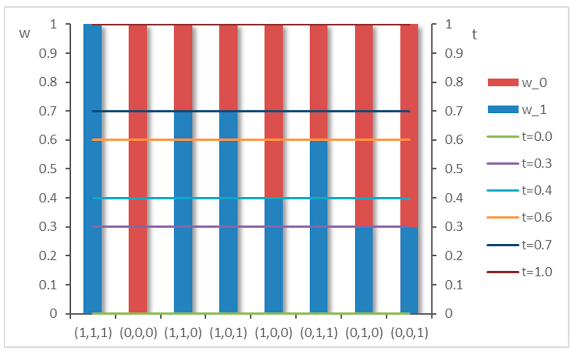
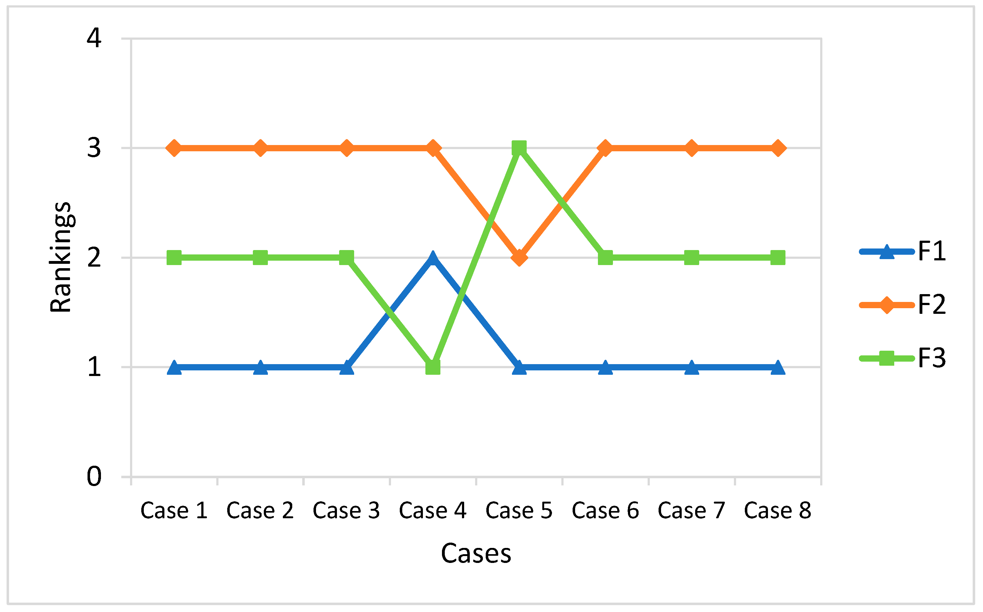
3.8. Sensitivity Analysis Regarding the Predetermined Expert Weights

In engineering applications, setting expert weights has a certain subjectivity, which may impact the final evaluation decision results. This section presents the sensitivity analysis regarding the predetermined expert weights further to validate the ship design evaluation and selection results. Eight cases are generated, as indicated in

Table 19. The case combinations with different expert weights.

Cases		${\mathit{w}}_1^{\mathit{p}}$	${\mathit{w}}_2^{\mathit{p}}$	${\mathit{w}}_3^{\mathit{p}}$
Case 1	Current	0.4	0.3	0.3
Case 2	Average	1/3	1/3	1/3
Case 3	$P_1$ High, The Rest Low	2/3	1/6	1/6
Case 4	$P_2$ High, The Rest Low	1/6	2/3	1/6
Case 5	$P_3$ High, The Rest Low	1/6	1/6	2/3
Case 6	$P_1$ Low, The Rest High	1/6	5/12	5/12
Case 7	$P_2$ Low, The Rest High	5/12	1/6	5/12
Case 8	$P_3$ Low, The Rest High	5/12	5/12	1/6

. The first case indicates the current expert weights. Case 2 is generated by allocating equal expert weights. The cases from 3 to 5 are generated by allocating the highest weight to one of the experts and the lower equal weight to the rest of the experts. Finally, the cases from 6 to 8 are generated by allocating the lowest weight to one of the experts and the higher equal weight to the rest. The rankings of the eight cases are presented in Figure 11. It is seen from Figure 11 that there are slightly different rankings of the alternative ship designs. For instance, design $F_3$ performs best in Case 4, and design $F_2$ performs better than $F_3$ in Case 5. However, design $F_1$ performs best in seven cases, and design $F_3$ performs better than $F_2$ in seven cases. The results indicate high engineering credibility in ship design evaluation and selection.

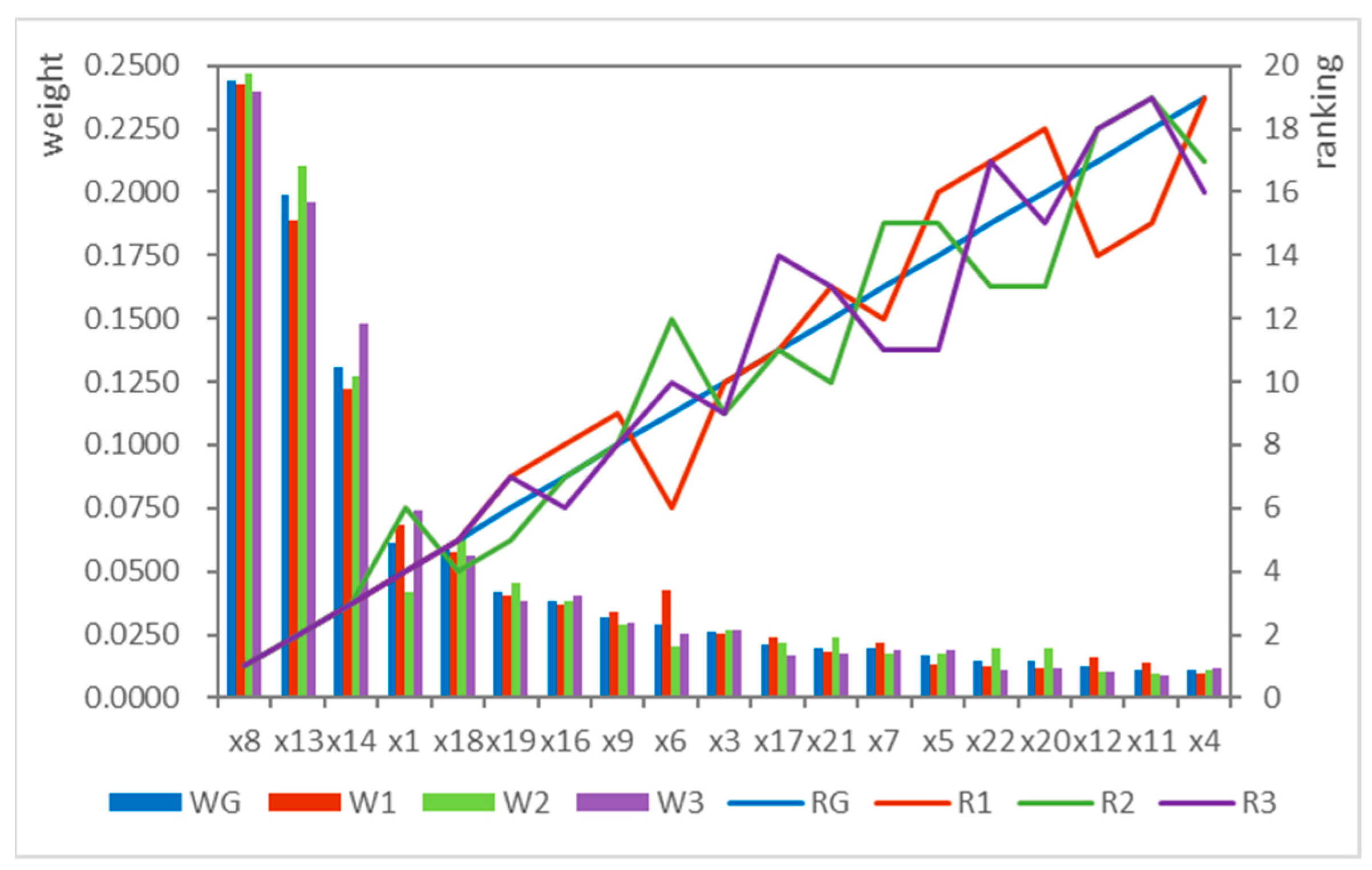
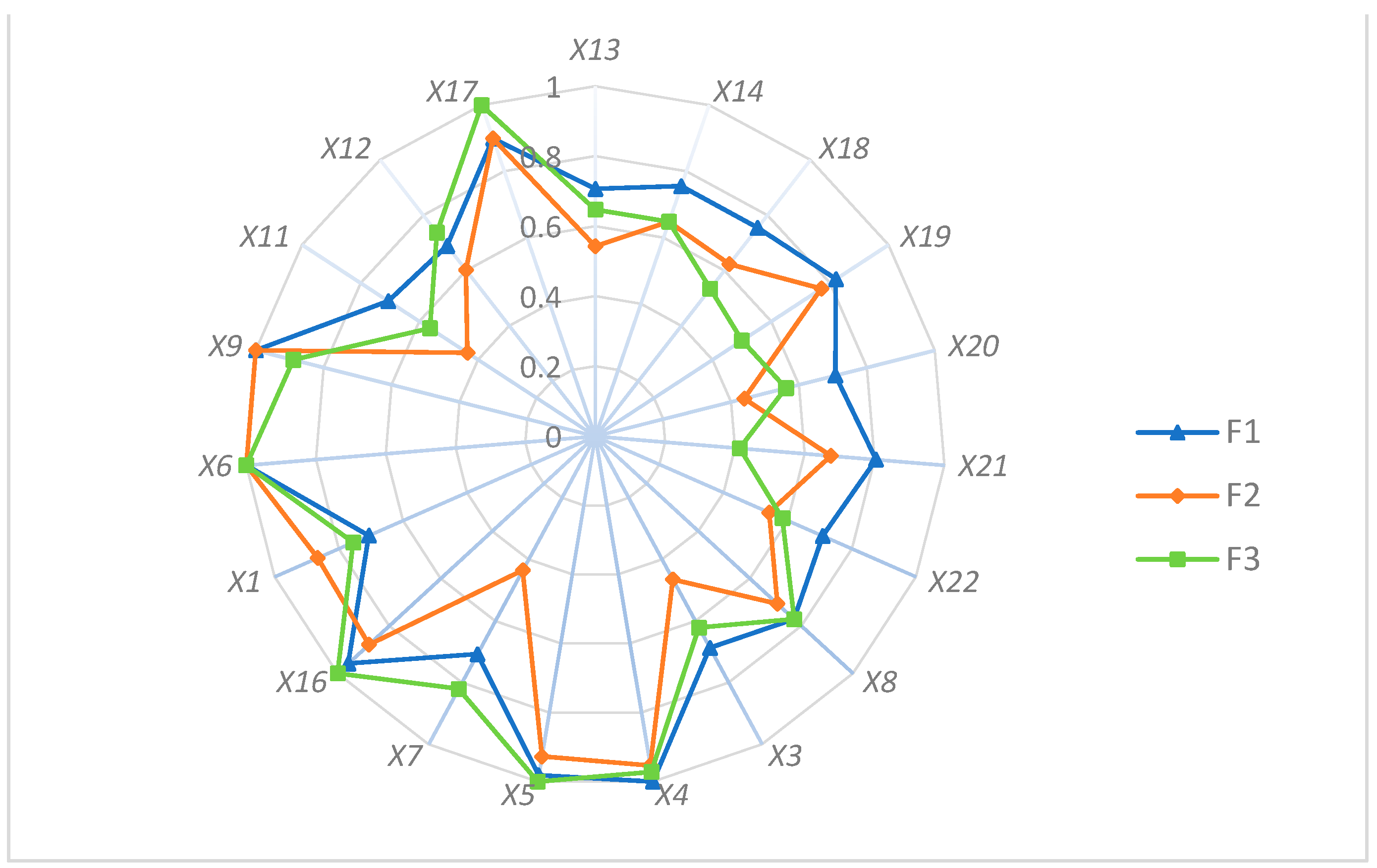
3.9. Comparative Analysis of Index Weights and Criteria Performances

Based on verifying the rationality of the evaluation results, valuable findings are obtained through the comparative analysis of the index weights of the assessment indicators and the criteria performances of the alternative ship designs.

Regarding ship-equipment environmental suitability, ship designers can evaluate and select optimal ship designs from the operational, electromagnetic, mechanical, and climatic aspects, which can be further divided into more detailed indicators. Figure 10 shows the global weights and rankings of the assessment indicators. It was observed that $X_8$ electromagnetic environment has the most considerable weight (24.4%), followed by $X_{13}$ draft (19.88%), $X_{14}$ course and attitude (13.11%), $X_1$ explosive gases (6.13%), $X_{18}$ waves in the cabin (5.91%), etc. The sum of the weight ratio of these five indicators has reached 69.43%. Therefore, ship designers should focus on special designs regarding these five indicators of ship-equipment environmental suitability. For example, when selecting shipborne electronic equipment, their spectrum allocation should be compatible with the management and control measures in time, space, frequency domain, and power supply. Furthermore, when determining principle dimensions, the designed draft should satisfy the requirements of the shipborne equipment regarding operational security and efficiency.

Figure 12 shows the criteria performances of each design solution, which contains much valuable information. For example, it is seen in Figure 12 that the first design $F_1$ performs better in the aspects of $X_8$ electromagnetic environment, $X_{13}$ draft, $X_{14}$ course and attitude, etc. However, there is still room for optimization in $X_5$ ship vibration (1.85%), $X_{16}$ tilting and swaying (4.32%), $X_{12}$ mold, oil mist, and salt spray (6.96%), and, particularly, $X_1$ explosive gases (22.54%), $X_7$ bumping (15.95%), and $X_{17}$ relative humidity (11.17%). By contrast, the third design $F_3$ performs best in $X_{17}$ relative humidity and $X_7$ bumping, whereas the second design $F_2$ performs best in $X_1$ explosive gases. Therefore, ship designers may take the above two ship designs as reference design solutions and carry out optimization design pertinently. More importantly, the selection of explosion-proof electrical equipment used in explosive dangerous places where explosive gases accumulate or spread must strictly satisfy the safety requirements. Furthermore, ship designers should strengthen communication and coordination with equipment manufacturers to specify the performance requirements of relevant shipborne equipment, such as communication antennas.

4. Conclusions

This paper investigated a hybrid MCDM framework for ship-equipment suitability evaluation using the improved ISM, AHP, and Fuzzy TOPSIS methods. In light of the outcomes, ship-equipment environmental suitability can be evaluated from the operational, electromagnetic, mechanical, and climatic aspects, where the electromagnetic environment is the most critical criterion. Furthermore, the optimal design solution needs to be improved regarding explosive gases, bumping, and relative humidity.

From the theoretical perspective, the ISM method is introduced to construct the evaluation index systems owing to its structural modeling and causal mapping capabilities. Furthermore, the scientific basis of the selected AHP and Fuzzy TOPSIS methods applied in ship design evaluation and selection is also verified systematically. In addition, benefitting from the extension to group decision-making settings and the verification and improvement of individual consistency and group consensus, the proposed methodology improves the rationality and operability of ship design evaluation and selection. In conclusion, it can promote the engineering credibility of the evaluation decision results and be applied to other group decision-making problems in ship design evaluation and selection.

The inherent complexity of warships makes it challenging to construct reasonable indicator systems and develop scientific evaluation decision methods. Although knowledge-based expert systems can be reasonable solutions, there are inevitable uncertainties and variances in expert opinions, especially in ship design evaluation and selection problems with numerous indicators and complex structures. This paper extended ship design evaluation and selection to group decision-making settings and TFNs environment, but the fuzzy sets and operators we applied are relatively simple. In future research, fuzzy MCDM methods and advanced information fusion operators may be introduced to ship design evaluation and selection to deal with the uncertainties and variances in expert opinions.

References

1. Hou, Y.; Huang, S.; Hu, Y.; Wang, W. Evaluation of warship based on relative entropy method. J. Shanghai Jiaotong Univ. 2012, 46, 1218–1229. [Google Scholar] [CrossRef]
2. Marini, C.D.; Fatchurrohman, N.; Azhari, A.; Suraya, S. Product development using QFD, MCDM and the combination of these two methods. IOP Conf. Ser. Mater. Sci. Eng. 2016, 114, 012089. [Google Scholar] [CrossRef]
3. Tan, K.H.; Noble, J.; Sato, Y.; Tse, Y.K. A marginal analysis guided technology evaluation and selection. Int. J. Prod. Econ. 2011, 131, 15–21. [Google Scholar] [CrossRef]
4. Díaz, H.; Loughney, S.; Wang, J.; Guedes Soares, C. Comparison of multicriteria analysis techniques for decision making on floating offshore wind farms site selection. Ocean Eng. 2022, 248, 110751. [Google Scholar] [CrossRef]
5. Nadkarni, R.R.; Puthuvayi, B. A comprehensive literature review of multi-criteria decision making methods in heritage buildings. J. Build. Eng. 2020, 32, 101841. [Google Scholar] [CrossRef]
6. Tan, T.; Mills, G.; Papadonikolaki, E.; Liu, Z. Combining multi-criteria decision making (MCDM) methods with building information modelling (BIM): A review. Autom. Constr. 2021, 121, 103451. [Google Scholar] [CrossRef]
7. Soner, O.; Celik, E.; Akyuz, E. Application of AHP and VIKOR methods under interval type 2 fuzzy environment in maritime transportation. Ocean Eng. 2017, 129, 107–116. [Google Scholar] [CrossRef]
8. Celik, E.; Akyuz, E. An interval type-2 fuzzy AHP and TOPSIS methods for decision-making problems in maritime transportation engineering: The case of ship loader. Ocean Eng. 2018, 155, 371–381. [Google Scholar] [CrossRef]
9. Xiong, W.; van Gelder, P.H.A.J.M.; Yang, K. A decision support method for design and operationalization of search and rescue in maritime emergency. Ocean Eng. 2020, 207, 107399. [Google Scholar] [CrossRef]
10. Li, Y.; Hu, Z. A review of multi-attributes decision-making models for offshore oil and gas facilities decommissioning. J. Ocean Eng. Sci. 2022, 7, 58–74. [Google Scholar] [CrossRef]
11. Boral, S.; Chakraborty, S. Failure analysis of CNC machines due to human errors: An integrated IT2F-MCDM-based FMEA approach. Eng. Fail. Anal. 2021, 130, 105768. [Google Scholar] [CrossRef]
12. Sugavaneswaran, M.; Prashanthi, B.; Rajan, J.A. A multi-criteria decision making method for vapor smoothening fused deposition modelling part. Rapid Prototyp. J. 2021, 28, 236–252. [Google Scholar] [CrossRef]
13. Sánchez-Lozano, J.M.; Fernández-Martínez, M.; Saucedo-Fernández, A.A.; Trigo-Rodriguez, J.M. Evaluation of NEA deflection techniques. A fuzzy Multi-Criteria decision making analysis for planetary defense. Acta Astronaut. 2020, 176, 383–397. [Google Scholar] [CrossRef]
14. Bazzocchi, M.C.F.; Sánchez-Lozano, J.M.; Hakima, H. Fuzzy multi-criteria decision-making approach to prioritization of space debris for removal. Adv. Space Res. 2021, 67, 1155–1173. [Google Scholar] [CrossRef]
15. Luthra, S.; Govindan, K.; Kannan, D.; Mangla, S.K.; Garg, C.P. An integrated framework for sustainable supplier selection and evaluation in supply chains. J. Clean. Prod. 2017, 140, 1686–1698. [Google Scholar] [CrossRef]
16. Georgiou, D.; Mohammed, E.S.; Rozakis, S. Multi-criteria decision making on the energy supply configuration of autonomous desalination units. Renew. Energy 2015, 75, 459–467. [Google Scholar] [CrossRef] [Green Version]
17. Lin, M.; Chen, Z.; Liao, H.; Xu, Z. ELECTRE II method to deal with probabilistic linguistic term sets and its application to edge computing. Nonlinear Dyn. 2019, 96, 2125–2143. [Google Scholar] [CrossRef]
18. Emeksiz, C.; Yüksel, A. A suitable site selection for sustainable bioenergy production facility by using hybrid multi-criteria decision making approach, case study: Turkey. Fuel 2022, 315, 123241. [Google Scholar] [CrossRef]
19. Lima Junior, F.R.; Osiro, L.; Carpinetti, L.C.R. A comparison between Fuzzy AHP and Fuzzy TOPSIS methods to supplier selection. Appl. Soft Comput. 2014, 21, 194–209. [Google Scholar] [CrossRef]
20. Xiao, F. A novel multi-criteria decision making method for assessing health-care waste treatment technologies based on D numbers. Eng. Appl. Artif. Intell. 2018, 71, 216–225. [Google Scholar] [CrossRef]
21. Liu, Y.; Eckert, C.M.; Earl, C. A review of fuzzy AHP methods for decision-making with subjective judgements. Expert Syst. Appl. 2020, 161, 113738. [Google Scholar] [CrossRef]
22. Lee, A.H.I.; Chen, H.H.; Kang, H.-Y. A conceptual model for prioritizing dam sites for tidal energy sources. Ocean Eng. 2017, 137, 38–47. [Google Scholar] [CrossRef]
23. Wang, L.; Zhang, H.Y.; Wang, J.Q.; Li, L. Picture fuzzy normalized projection-based VIKOR method for the risk evaluation of construction project. Appl. Soft Comput. 2018, 64, 216–226. [Google Scholar] [CrossRef]
24. Ayadi, H.; Hamani, N.; Kermad, L.; Benaissa, M. Novel fuzzy composite indicators for locating a logistics platform under sustainability perspectives. Sustainability 2021, 13, 3891. [Google Scholar] [CrossRef]
25. Hashemi, H.; Mousavi, S.; Zavadskas, E.; Chalekaee, A.; Turskis, Z. A new group decision model based on grey-intuitionistic fuzzy-ELECTRE and VIKOR for contractor assessment problem. Sustainability. 2018, 10, 1635. [Google Scholar] [CrossRef] [Green Version]
26. Jana, C.; Pal, M. Extended bipolar fuzzy EDAS approach for multi-criteria group decision-making process. Comput. Appl. Math. 2021, 40, 9. [Google Scholar] [CrossRef]
27. Jana, C.; Pal, M.; Wang, J. A robust aggregation operator for multi-criteria decision-making method with bipolar fuzzy soft environment. Iran. J. Fuzzy Syst. 2019, 16, 1–16. [Google Scholar]
28. Joshi, B.P.; Gegov, A. Confidence levelsq-rung orthopair fuzzy aggregation operators and its applications to MCDM problems. Int. J. Intell. Syst. 2019, 35, 125–149. [Google Scholar] [CrossRef]
29. Joshi, B.P. Pythagorean fuzzy average aggregation operators based on generalized and group-generalized parameter with application in MCDM problems. Int. J. Intell. Syst. 2019, 34, 895–919. [Google Scholar] [CrossRef]
30. Jana, C.; Senapati, T.; Pal, M. Pythagorean fuzzy Dombi aggregation operators and its applications in multiple attribute decision-making. Int. J. Intell. Syst. 2019, 34, 2019–2038. [Google Scholar] [CrossRef]
31. Joshi, B.P. Moderator intuitionistic fuzzy sets with applications in multi-criteria decision-making. Granul. Comput. 2017, 3, 61–73. [Google Scholar] [CrossRef]
32. Moustafa, E.B.; Elsheikh, A. Predicting Characteristics of Dissimilar Laser Welded Polymeric Joints Using a Multi-Layer Perceptrons Model Coupled with Archimedes Optimizer. Polymers 2023, 15, 233. [Google Scholar] [CrossRef]
33. Elsheikh, A.H. Applications of machine learning in friction stir welding: Prediction of joint properties, real-time control and tool failure diagnosis. Eng. Appl. Artif. Intell. 2023, 121, 105961. [Google Scholar] [CrossRef]
34. Elsheikh, A. Bistable Morphing Composites for Energy-Harvesting Applications. Polymers 2022, 14, 1893. [Google Scholar] [CrossRef]
35. Elsheikh, A.H.; El-Said, E.M.S.; Abd Elaziz, M.; Fujii, M.; El-Tahan, H.R. Water distillation tower: Experimental investigation, economic assessment, and performance prediction using optimized machine-learning model. J. Clean. Prod. 2023, 388, 135896. [Google Scholar] [CrossRef]
36. Khoshaim, A.B.; Moustafa, E.B.; Bafakeeh, O.T.; Elsheikh, A.H. An Optimized Multilayer Perceptrons Model Using Grey Wolf Optimizer to Predict Mechanical and Microstructural Properties of Friction Stir Processed Aluminum Alloy Reinforced by Nanoparticles. Coatings 2021, 11, 1476. [Google Scholar] [CrossRef]
37. Celik, M.; Er, I.D. Fuzzy axiomatic design extension for managing model selection paradigm in decision science. Expert Syst. Appl. 2009, 36, 6477–6484. [Google Scholar] [CrossRef]
38. Kurka, T.; Blackwood, D. Selection of MCA methods to support decision making for renewable energy developments. Renew. Sustain. Energy Rev. 2013, 27, 225–233. [Google Scholar] [CrossRef]
39. Cinelli, M.; Coles, S.R.; Kirwan, K. Analysis of the potentials of multi criteria decision analysis methods to conduct sustainability assessment. Ecol. Indic. 2014, 46, 138–148. [Google Scholar] [CrossRef] [Green Version]
40. Saaty, T.L.; Ergu, D. When is a decision-making method trustworthy? Criteria for evaluating multi-criteria decision-making methods. Int. J. Inf. Technol. Decis. Mak. 2015, 14, 1171–1187. [Google Scholar] [CrossRef]
41. Chen, T.Y. Comparative analysis of SAW and TOPSIS based on interval-valued fuzzy sets: Discussions on score functions and weight constraints. Expert Syst. Appl. 2012, 39, 1848–1861. [Google Scholar] [CrossRef]
42. Chang, Y.H.; Yeh, C.H.; Chang, Y.W. A new method selection approach for fuzzy group multicriteria decision making. Appl. Soft Comput. 2013, 13, 2179–2187. [Google Scholar] [CrossRef]
43. Madhu, P.; Sowmya Dhanalakshmi, C.; Mathew, M. Multi-criteria decision-making in the selection of a suitable biomass material for maximum bio-oil yield during pyrolysis. Fuel 2020, 277, 118109. [Google Scholar] [CrossRef]
44. Sałabun, W.; Wątróbski, J.; Shekhovtsov, A. Are MCDA methods benchmarkable? A comparative study of TOPSIS, VIKOR, COPRAS, and PROMETHEE II methods. Symmetry. 2020, 12, 1549. [Google Scholar] [CrossRef]
45. Cicek, K.; Celik, M.; Ilker Topcu, Y. An integrated decision aid extension to material selection problem. Mater. Des. 2010, 31, 4398–4402. [Google Scholar] [CrossRef]
46. Wątróbski, J.; Jankowski, J.; Ziemba, P.; Karczmarczyk, A.; Zioło, M. Generalised framework for multi-criteria method selection. Omega 2019, 86, 107–124. [Google Scholar] [CrossRef]
47. Cinelli, M.; Kadziński, M.; Gonzalez, M.; Słowiński, R. How to support the application of multiple criteria decision analysis? Let us start with a comprehensive taxonomy. Omega 2020, 96, 102261. [Google Scholar] [CrossRef]
48. Saaty, T.L. A scaling method for priorities in hierarchical structures. J. Math. Psychol. 1977, 15, 234–281. [Google Scholar] [CrossRef]
49. Rezaei, J. Best-worst multi-criteria decision-making method. Omega 2015, 53, 49–57. [Google Scholar] [CrossRef]
50. Mohammed, M.A.; Abdulkareem, K.H.; Al-Waisy, A.S.; Mostafa, S.A.; Al-Fahdawi, S.; Dinar, A.M.; Alhakami, W.; Baz, A.; Al-Mhiqani, M.N.; Alhakami, H.; et al. Benchmarking methodology for selection of optimal COVID-19 diagnostic model based on entropy and TOPSIS methods. IEEE Access 2020, 8, 99115–99131. [Google Scholar] [CrossRef]
51. Bozóki, S.; Fülöp, J.; Poesz, A. On reducing inconsistency of pairwise comparison matrices below an acceptance threshold. Cent. Eur. J. Oper. Res. 2015, 23, 849–866. [Google Scholar] [CrossRef] [Green Version]
52. Negahban, A. Optimizing consistency improvement of positive reciprocal matrices with implications for Monte Carlo Analytic Hierarchy Process. Comput. Ind. Eng. 2018, 124, 113–124. [Google Scholar] [CrossRef]
53. Temesi, J. An interactive approach to determine the elements of a pairwise comparison matrix. Cent. Eur. J. Oper. Res. 2019, 27, 533–549. [Google Scholar] [CrossRef]
54. Xu, K.; Xu, J.P. A direct consistency test and improvement method for the analytic hierarchy process. Fuzzy Optim. Decis. Mak. 2020, 19, 359–388. [Google Scholar] [CrossRef]
55. Cao, D.; Leung, L.C.; Law, J.S. Modifying inconsistent comparison matrix in analytic hierarchy process: A heuristic approach. Decis. Support Syst. 2008, 44, 944–953. [Google Scholar] [CrossRef]
56. Kou, G.; Ergu, D.; Shang, J. Enhancing data consistency in decision matrix: Adapting Hadamard model to mitigate judgment contradiction. Eur. J. Oper. Res. 2014, 236, 261–271. [Google Scholar] [CrossRef] [Green Version]
57. Mazurek, J.; Perzina, R.; Strzalka, D.; Kowal, B. A new step-by-step (SBS) algorithm for inconsistency reduction in pairwise comparisons. IEEE Access 2020, 8, 135821–135828. [Google Scholar] [CrossRef]
58. Mazurek, J.; Perzina, R.; Strzalka, D.; Kowal, B.; Kuras, P. A numerical comparison of iterative algorithms for inconsistency reduction in pairwise comparisons. IEEE Access 2021, 9, 62553–62561. [Google Scholar] [CrossRef]
59. Saaty, T.L. Decision-making with the AHP: Why is the principal eigenvector necessary. Eur. J. Oper. Res. 2003, 145, 85–91. [Google Scholar] [CrossRef]
60. Escobar, M.T.; Moreno-Jiménez, J.M. Aggregation of individual preference structures in AHP-group decision making. Group Decis. Negot. 2006, 16, 287–301. [Google Scholar] [CrossRef]
61. MarÍa, J.; JimÉnez, M.; Joven, J.A.; Pirla, A.R.; Lanuza, A.T. A spreadsheet module for consistent consensus building in AHP-group decision making. Group Decis. Negot. 2005, 14, 89–108. [Google Scholar] [CrossRef]
62. Moreno-Jiménez, J.M.; Aguarón, J.; Escobar, M.T. The core of consistency in AHP-group decision making. Group Decis. Negot. 2008, 17, 249–265. [Google Scholar] [CrossRef]
63. Altuzarra, A.; Moreno-Jiménez, J.M.; Salvador, M. Consensus building in AHP-group decision making: A Bayesian approach. Oper. Res. 2010, 58, 1755–1773. [Google Scholar] [CrossRef]
64. Aguarón, J.; Escobar, M.T.; Moreno-Jiménez, J.M. The precise consistency consensus matrix in a local AHP-group decision making context. Ann. Oper. Res. 2016, 245, 245–259. [Google Scholar] [CrossRef]
65. Escobar, M.T.; Aguarón, J.; Moreno-Jiménez, J.M. Some extensions of the precise consistency consensus matrix. Decis. Support Syst. 2015, 74, 67–77. [Google Scholar] [CrossRef]
66. Hamid-Mosaku, I.A.; Oguntade, O.F.; Ifeanyi, V.I.; Balogun, A.-L.; Jimoh, O.A. Evolving a comprehensive geomatics multi-criteria evaluation index model for optimal pipeline route selection. Struct. Infrastruct. Eng. 2020, 16, 1382–1396. [Google Scholar] [CrossRef]
67. Alawneh, R.; Ghazali, F.; Ali, H.; Sadullah, A.F. A novel framework for integrating United Nations Sustainable Development Goals into sustainable non-residential building assessment and management in Jordan. Sustain. Cities Soc. 2019, 49, 101612. [Google Scholar] [CrossRef]
68. Mohandes, S.R.; Zhang, X. Towards the development of a comprehensive hybrid fuzzy-based occupational risk assessment model for construction workers. Saf. Sci. 2019, 115, 294–309. [Google Scholar] [CrossRef]
69. Zhao, H.; Guo, S.; Zhao, H. Comprehensive assessment for battery energy storage systems based on fuzzy-MCDM considering risk preferences. Energy 2019, 168, 450–461. [Google Scholar] [CrossRef]
70. Liu, A.; Zhao, Y.; Meng, X.; Zhang, Y.L. A three-phase fuzzy multi-criteria decision model for charging station location of the sharing electric vehicle. Int. J. Prod. Econ. 2020, 225, 107572. [Google Scholar] [CrossRef]
71. Warfield, J.N. Developing Interconnection Matrices in Structural Modeling. IEEE Trans. Syst. Man Cybern. 1974, 1, 81–87. [Google Scholar] [CrossRef] [Green Version]
72. Ghobakhloo, M. Industry 4.0, digitization, and opportunities for sustainability. J. Clean. Prod. 2020, 252, 119869. [Google Scholar] [CrossRef]
73. Luthra, S.; Kumar, S.; Kharb, R.; Ansari, M.F.; Shimmi, S.L. Adoption of smart grid technologies: An analysis of interactions among barriers. Renew. Sustain. Energy Rev. 2014, 33, 554–565. [Google Scholar] [CrossRef]
74. Ren, J. New energy vehicle in China for sustainable development: Analysis of success factors and strategic implications. Transp. Res. Part D 2018, 59, 268–288. [Google Scholar] [CrossRef]
75. Kaswan, M.S.; Rathi, R. Analysis and modeling the enablers of Green Lean Six Sigma implementation using Interpretive Structural Modeling. J. Clean. Prod. 2019, 231, 1182–1191. [Google Scholar] [CrossRef]
76. Tan, T.; Chen, K.; Xue, F.; Lu, W. Barriers to building information modeling (BIM) implementation in China’s prefabricated construction: An interpretive structural modeling (ISM) approach. J. Clean. Prod. 2019, 219, 949–959. [Google Scholar] [CrossRef]
77. Williams, C.C. A note on the analysis of subjective judgment matrices. J. Math. Psychol. 1985, 29, 387–405. [Google Scholar] [CrossRef]
78. Aguarón, J.; Escobar, M.T.; Moreno-Jiménez, J.M. Reducing inconsistency measured by the geometric consistency index in the analytic hierarchy process. Eur. J. Oper. Res. 2021, 288, 576–583. [Google Scholar] [CrossRef]
79. Aguarón, J.; Moreno-Jiménez, J.M. The geometric consistency index: Approximated thresholds. Eur. J. Oper. Res. 2003, 147, 137–145. [Google Scholar] [CrossRef]
80. Liu, F.; Shi, D.; Xiao, Y.; Zhang, T.; Sun, J. Comprehensive evaluation on space information network demonstration platform based on tracking and data relay satellite system. Sensors 2020, 20, 5437. [Google Scholar] [CrossRef]
81. Grošelj, P.; Zadnik Stirn, L. Acceptable consistency of aggregated comparison matrices in analytic hierarchy process. Eur. J. Oper. Res. 2012, 223, 417–420. [Google Scholar] [CrossRef]
82. Liu, F.; Zhang, W.G.; Wang, Z.X. A goal programming model for incomplete interval multiplicative preference relations and its application in group decision-making. Eur. J. Oper. Res. 2012, 218, 747–754. [Google Scholar] [CrossRef]
83. Wu, Z.; Tu, J. Managing transitivity and consistency of preferences in AHP group decision making based on minimum modifications. Inf. Fusion 2021, 67, 125–135. [Google Scholar] [CrossRef]
84. Hwang, C.L.; Yoon, K.; Hwang, C.L.; Yoon, K. Multiple attribute decision making. Lect. Notes Econ. Math. Syst. 1981, 404, 287–288. [Google Scholar] [CrossRef]
85. Chen, C.T. Extensions of the TOPSIS for group decision-making under fuzzy environment. Fuzzy Sets Syst. 2000, 114, 1–9. [Google Scholar] [CrossRef]
86. Zadeh, L.A. Fuzzy sets. Inf. Control 1965, 8, 338–353. [Google Scholar] [CrossRef] [Green Version]
87. Miller, G.A. The magical number seven, plus or minus two: Some limits on our capacity to process information. Psychol. Rev. 1956, 63, 81–97. [Google Scholar] [CrossRef] [Green Version]
Figure 1. The framework of research methodology.
Jmse 11 00607 g001
Figure 2. Flow chart of the improved ISM technique.
Jmse 11 00607 g002
Figure 3. Flow chart of the group consensus improvement algorithm.
Jmse 11 00607 g003
Figure 4. Characteristics of general decision problems.
Jmse 11 00607 g004
Figure 5. Flow chart of the improved AHP technique.
Jmse 11 00607 g005
Figure 6. Flow chart of the individual consistency improvement algorithm.
Jmse 11 00607 g006
Figure 7. Linguistic scales for rating the criteria performances.
Jmse 11 00607 g007
Figure 8. Evaluation index system of ship-equipment environmental suitability.
Jmse 11 00607 g008
Figure 9. Expert judgment aggregation with different thresholds.
Jmse 11 00607 g009
Figure 10. Global weights and their rankings.
Jmse 11 00607 g010
Figure 11. The ranking changes in the sensitivity analysis.
Jmse 11 00607 g011
Figure 12. Criteria performances of each design solution.
Jmse 11 00607 g012