Study of a Method for Drivability of Monopile in Complex Stratified Soil

Abstract

At present, there is no commonly used method for predicting soil resistance to the driving (SRD) of monopiles, because all available methods are developed based on an installed offshore pile with a diameter of 2–3 m. In addition, due to the complexity of soil profiles in situ, the accuracy of methods used is often not stable under different soil conditions. Based on two typical stratified soil conditions of offshore wind farms in the East China Sea, which are clay-interlayered sand and sand-interlayered clay where, according to the pile driving records of the monopiles in sites, the SRD is obtained by back analysis using the method of the wave equation. At the same time, SRD is also calculated using Steven and Alm methods and compared with that of the back analysis. The results show that the SRDs from the Steven and Alm methods are basically consistent with that of the back analysis, but the predicted SRD of the clay layer is higher than that of back analysis, while the predicted SRD of the sand layer is lower. Based on the characteristics of SRD in different soil layers, a modified method for calculating unit friction in clay and the unit end resistance in sand is proposed for stratified soil, and the error between SRD of the proposed method and of the back analysis was approximately 20%. It could be helpful to improve the accuracy of the monopile drivability analysis in stratified soil.

1. Introduction

Offshore wind turbines are elevated over the sea level with different types of foundations, and they are considered as a reliable source of renewable energy. In recent years, although the floating offshore wind turbine is considered more competitive, on which many studies have been carried out [1,2], the scale of fixed bottom wind farms is still expanding. Novel foundations for offshore wind turbines have been used, such as the helical pile due to its fast installation, high uplift capacity, and convenience for recycling [3,4].

Byrne proposed the use of helical piles as the foundation for multi-footing structure [5]. The design parameters were studied to evaluate its behavior in clay [6,7,8]. However, the monopile is still the most commonly used foundation for offshore wind turbines because of its simple design and the fact it works well in different kinds of soils [9]. Its stability under complex loading is of concern to many people [10,11]. In addition, because a monopile is typically driven into the seabed with a large hydraulic hammer, the accuracy of pile drivability predictions is critical to the successful installation for pile foundation.

At present, Smith’s drivability model, based on one dimensional wave equation, is used widely to evaluate pile drivability, which requires the consideration of the pile model, hammer model, and soil model [12]. As an open-ended steel pile, a monopile could be place by a plugged, partially plugged, or unplugged (coring) driving manner, and the coring mode of penetration is dominant, particularly for larger diameter piles [13]. For the hammer model, the hydraulic impact hammer is popular since it is more efficient. For the soil model, the soil resistance is often modeled as the sum of dynamic and static components [14]. When performing pile drivability analysis, the accurate determination of the soil resistance to driving (SRD) is very important.

SRD can be calculated based on indoor tests results or Cone penetration test (CPT) results. It is the sum of the skin friction and tip resistance, which is similar to the computation of the axial capacity of the pile and could be obtained by reducing the axial capacity of the pile determined according to the American Petroleum Institute (API) [15]. Steven et al. (1982) proposed the method that is often used to date to calculate the SRD under plugged and unplugged (coring) conditions for sand and clay, respectively [16]. Toolan and Fox (1977) proposed that the unit tip resistance and unit skin friction for SRD could be determined by the tip resistance of CPT ($q_c$). They suggested that, for piles in the sand, the unit tip resistance and unit skin friction could be obtained as a weighted average and a fraction of $q_c$, respectively [17]. The method proposed by Alm et al. (2001) is a popular CPT-based method which is also currently in use. Based on pile driving records from North Sea, Alm and Hamre developed a method to estimate the SRD under coring conditions for dense to very dense sand as well as clay [18]. Based on Alm’s method, Schneider et al. (2010) correlated CPT results with soil properties and proposed a method to calculate the SRD for open-ended piles in very dense sands [19]. Based on variety of axial capacity approaches (IC-05 [20], UWA-05 [21], and Fugro-05 [22]), Prendergast et al. (2020) proposed the modified IC-05, UWA-05, and Fugro-05 to calculate the SRD in sand [23].

The methods mentioned above were all developed based on an installed offshore pile with a diameter of 2–3 m [24]. However, for a monopile, which can be either categorized as a regular monopile (5–6 m), XL monopile (6–8 m), XXL monopile (8–11 m), and mega monopile (more than 11 m) according to its diameter [25], there are no standardized methods for calculating the SRD. At present, the methods used for monopile drivability analysis are often the same as those used in the oil and gas industry. Because the drivability analysis method heavily relies on experience and approaches used in practice, this led to low confidence in prediction results.

In order to evaluate the accuracy of the current method for large-diameter monopiles, Ferreira (2016) calculated the SRD of the XL monopile with a different method, and concluded that the CPT-based methods work well when dealing with clean sands, however, when facing more complex soil mixtures, the methods did not prove reliable [26]. Davidson et al. (2018) studied the SRD of the monopile with a 5 m diameter in predominantly stiff fissured clay, and found that the soil sensitivity significantly affected the magnitude of the SRD and proposed an alternative method to account for the soil sensitivity in SRD calculations [27]. Byrne et al. (2018) used a monopile with 4.2 m diameter installation records from the North Sea to study the influence of mobilized base resistance and aging on the pile drivability according to CPT-based axial capacity approaches, and suggested that the modified IC-05 and the modified UWA-05 could provide an estimate of the expected behavior of a monopile under driving to an acceptable industry tolerance for the sand layer [28]. Perikleous et al. (2019) made a comparison of the SRD from three prediction methods with respect to the back analysis performed for monopiles (6–8 m) in the Irish Sea, and found that the accuracy of the Alm method is related to the depth of soil layers whilst the Steven method under-predicted the SRD [29]. Based on the back analysis of over 200 monopile driving records, Maynard (2019) found that Alm’s method performed well in predicting the SRD of the monopile if the soil conditions at the site resemble those of the site conditions of the 2–3 m pile. However, it was shown to overpredict the SRD in older, higher-OCR, higher-plasticity clays and denser silty sands, and underpredict the SRD in normally to marginally over-consolidated clays with lower plasticity [30]. It could be found that, although some studies have been performed on the SRD of the monopile, the ability to obtain a fair estimate of the monopile drivability remains a challenge, and it was suggested that lessons could be learned from the installation of the piles for different areas.

In this paper, two typical sites with stratified soil were selected from 37 boreholes in the East China Sea. Based on the pile driving records of monopiles with diameters of 6–9 m driving in the stratified soil, the back analysis was performed to obtain the SRD, and the characteristics of the SRD on the stratified soil were analyzed. Based on the results from the back analysis and the SRD calculated using the Alm and Steven methods, a modified method is proposed to calculate the SRD of monopiles in stratified soil. It can be used to calculate SRD in a site with clay-interlayered sand or sand-interlayered clay, and will be helpful to a drivability assessment of monopiles for a wide variety of sites.

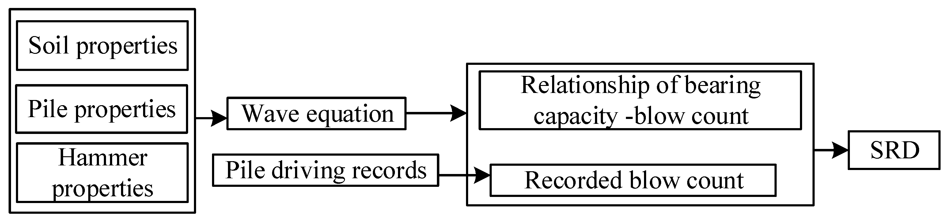
2. SRD Obtained by Back Analysis

The SRD from the back analysis was obtained using the method of wave equation with the pile driving records (blow count) in situ. The wave equation is often used to investigate the dynamic behavior of pile during driving.

$$\frac{1}{c^2}\left(\frac{{\partial }^{2}u}{\partial t^2}\right)=\left(\frac{{\partial }^{2}u}{\partial x^2}\right)$$

(1)

where x is the coordinate position of the pile section; u is the vertical displacement of the pile; t is the time; c is the wave speed and $c={(E/\rho )}^{0.5}$; $\rho$ is the density of the pile; and E is the elastic modulus.

In order to calculate the stress wave propagation during pile driving, the hammer- pile–soil system is divided into multiple elements, each of which is composed of a mass block and a spring. The piling process is divided with time intervals Δt, in each of which the physical quantity remains unchanged. To solve Equation (1), Smith deduced the five following basic difference equations [14]:

$$d_n^m=d_{{}_n}^{m-1}+v_n^{m-1}\Delta t$$

(2)

$$c_n^m=d_{{}_n}^m-d_{n+1}^m$$

(3)

$$F_n^m=c_{{}_n}^m{K}_n$$

(4)

$$Z_n^m=F_{{}_{n-1}}^m+F_n^m-R_n$$

(5)

$$v_n^m=v_{{}_n}^{m-1}+z_n^m\frac{g\Delta t}{W_n}$$

(6)

where d is the displacement of the mass block; v is the speed of the mass block; F is the spring force; c is the spring compression deformation; K is the stiffness of the spring; Z is accelerating force; R is the soil resistance to driving (SRD); W is the weight of the mass block; the superscript m is the serial number of the time interval; and the subscript n is the serial number of the block. It could be found that, when the soil resistance to driving R is known, the relationship between R and the corresponding penetration c or the number of blows required per unit penetration can be obtained by solving the above difference equation, which is the exactly the same as that used for obtaining the pile drivability.

Therefore, it is very important to determine the reasonable value of SRD when the pile drivability analysis is performed. The back analysis is often used to obtain the SRD from the pile driving records. With the equation analysis software GRLWEAP (2010), the relationships between SRD and the blow count could be established. The flow chart of the back analysis procedure is shown in Figure 1.

It should be noted that, since the hammer energy per blow often changes with the increment in pile penetration depth in practice, and the relationship between the SRD and blow count changed with the hammer energy, it is necessary to establish the relationships between SRD and blow count under each hammer’s energy used in pile driving.

3. Methods for Predicted SRD

As mentioned above, there is no commonly used method for predicting the SRD of monopiles, so different researchers have suggested different methods to calculate the SRD, such as Steven’s method, Alm’s method, modified IC-05 method, modified UWA-05 method, etc. Among them, the most commonly used methods are the Steven and Alm methods. In this paper, the accuracies of the Steven method and Alm methods, which are often used in practice, in stratified soil are discussed at first and a modified method for stratified soil is proposed. The two methods are shown as follows:

(1)

Steven’s Method (1982)

Based on the soil properties by indoor tests, Steven (1982) proposed the method for both unplugged (coring) and plugged conditions, and the lower and upper bound values of the SRD were calculated under each condition. Considering that the diameter of the monopiles in this study is approximately 9 m, the method under unplugged conditions is used.

Under unplugged conditions, the internal and external skin friction is considered and combined with annular end bearing. The lower and upper bound values can be calculated with Equations (7) and (8) as follow,

Lower value under coring:

$$SRD=1.5Q_f+Q_{tip}$$

(7)

Upper value under coring:

$$SRD=2.0Q_f+Q_{tip}$$

(8)

where $Q_f$ is the total outside friction of a pile and $Q_{tip}$ is the bearing capacity on the pile annulus. The unit friction resistance and unit end resistance for clay and sand can be calculated with the methods proposed by the API method.

It should be noted that, considering the influence of pile driving on resistance, the unit friction resistance for clay should be multiplied by a factor $F_p$ as follows

$$F_p=0.5\cdot {(OCR)}^{0.3}$$

(9)

The unit friction resistance for sand is the same as that proposed by API,

$$f_{sf}=K\cdot {\sigma }_v^{\prime }\cdot \tan \delta$$

(10)

where $f_{sf}$ is the unit friction resistance for sand, $K$ is the coefficient of lateral pressure, ${\sigma }_v^{\prime }$ is the effective overburden stress. and $\delta$ is the external friction angle. However, Steven et al. suggested that $K=0.7$.

(2)

Alm’s Method (2001)

The SRD is the sum of the friction resistance and end resistance, where the friction resistance accounts for both the internal and external shaft frictions, and the end resistance is applied to the annular area of the pile. Alm suggested that the upper bound resistance is calculated as 1.25 times the best estimate.

The unit friction resistance was calculated by

$$f_s=f_{sres}+(f_{si}-f_{sres})\cdot e^{k(d-p)}$$

(11)

where $f_s$ is the unit friction resistance; $f_{sres}$ is the residual friction resistance; $f_{si}$ is the initial friction resistance; $d$ is the depth to the soil layer; $p$ is the pile penetration depth; and $k$ is the shape degradation factor.

$$k=\frac{1}{80}{(q_c/{\sigma }_v\prime )}^{0.5}$$

(12)

$q_c$ is cone tip resistance.

For sand, each parameter can be calculated with

$$f_{s,i}=K\cdot {\sigma }_v^{\prime }\cdot \tan \delta ,\begin{array}{cc}& \end{array}K\cdot {\sigma }_v^{\prime }=0.0132\cdot q_c\cdot {\left(\frac{{\sigma }_v^{\prime }}{p_a}\right)}^{0.13}$$

(13)

$$f_{sres}=0.2f_{si}$$

(14)

For clay, these are

$$f_{s,i}=f_f$$

(15)

$$f_{sres}=0.004q_c(1-0.0025q_c/{\sigma }_v\prime )$$

(16)

The unit end resistance was calculated by

For sand,

$$q_{tip}=0.15\cdot q_c\cdot {\left(\frac{q_c}{{\sigma }_v^{\prime }}\right)}^{0.2}$$

(17)

For clay,

$$q_{tip}=0.6\cdot q_c$$

(18)

where $f_f$ is the sleeve friction of CPT.

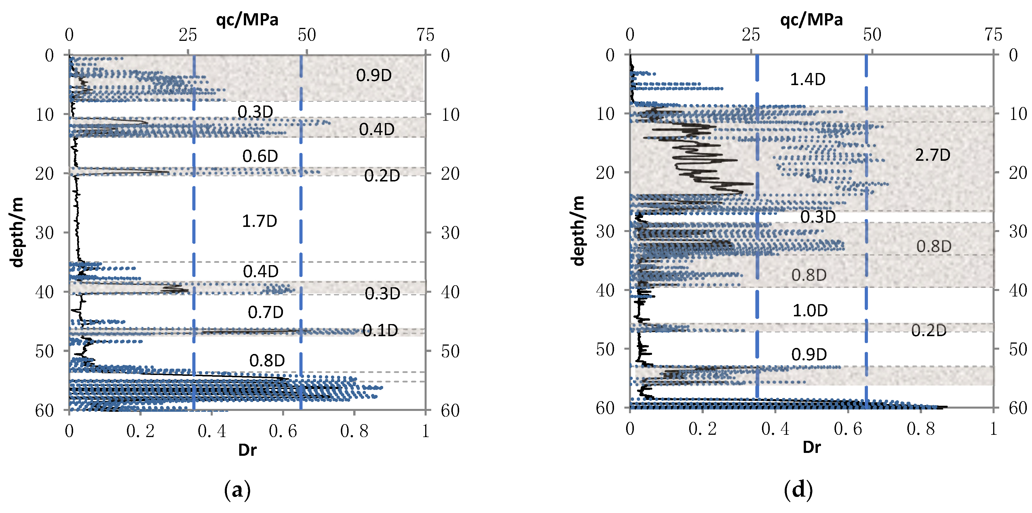
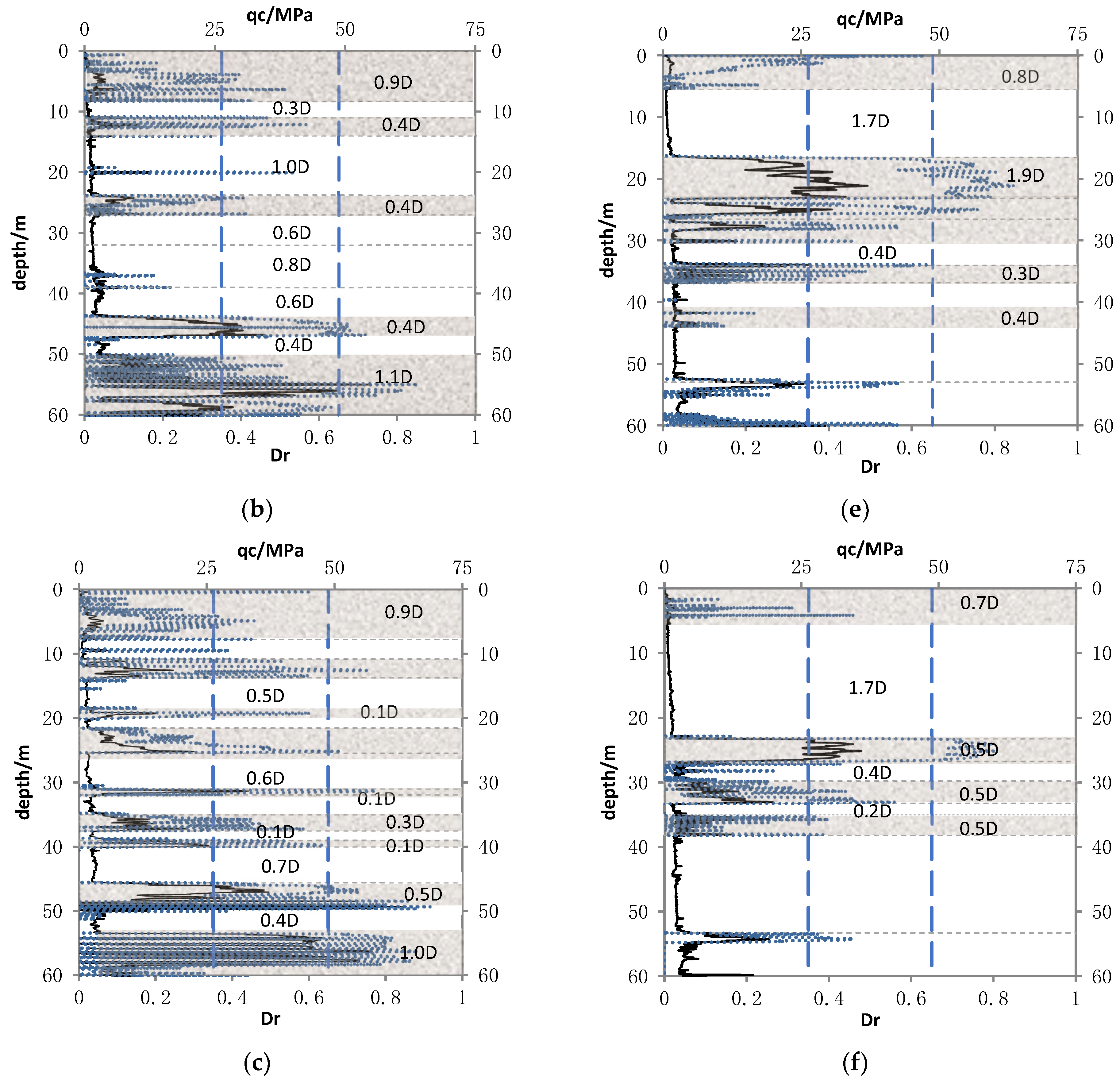
4. Pile Database

Two typical stratified soil profiles were selected from the installation database assembled by the Key Laboratory of Far-shore Wind Power Technology. These are (1) Clay-interlayered sand, which means that clay and sand occur alternately, and the continuously distributed clay layer contains thin sand layers with a thickness of 0.1–0.5 D when the depth exceeds 10 m. This is named Case 1. (2) Sand-interlayered clay, which means that the clay and sand occur alternately, and the continuously distributed sand contains thin clay layers with a thickness of 0.1–0.5 D. This is named Case 2.

Three sets of data are used for the analysis in each case and shown in

Table 1. Monopiles used for back-analysis.

No.	Case 1 (a)	Case 1 (b)	Case 1 (c)	Case 2 (a)	Case 2 (b)	Case 2 (c)
Diameter (m)	8.8	9.0	8.8	6.5	6.5	7.0
Thickness at tip (mm)	94	96	94	90	90	80
Length (m)	108.8	107.0	101.9	69.0	75.0	82.3
Penetration underweight pile + hammer (m)	18.0	31.5	18.7	12.3	18.2	18.7
Pile running (m)	18.5–36.0	/	19.5–36.5	/	/	/
Final penetration depth (m)	54.0	52.0	47.7	38.9	44.9	52.2
Hammer	MHU3500	MHU 3500	MHU3500	MHU1900	IHC1400	IHC1400
Dominant soil	Clay, Su = 16–115 Kpa			Sand, most are MED DENSE sand
Interlayer soil	The thickness of each sand layer is about 0.1–0.5 D			The thickness of each clay layer is about 0.1–0.4 D

and Figure 2, respectively. For Case 1, all the data from Project SQ; and for Case 2, all the data from Project BH are used. Table 1 gives the primary pile, hammer, and soil conditions of each example. In Table 1, it could be found that, under the self-weight of the pile and the hammer, the penetrated depth of all piles in the soil is more than 10 m, whilst pile running happened in Case 1 (a) and (c). If considering pile running, for clay-based Case 1, the initial pile driving depth is more than 30 m. The soil layers concerned in this study refer to the soil layer where the pile is penetrated by driving, but not including the layers where piles are penetrated by the pile and hammer self-weight and pile running.

Figure 2 shows the in depth profile of the end resistance of CPT qc. The shaded area refers to the sand layer, the blank area refers to the clay layer, and the thickness normalized with D (pile diameter) of each layer is marked.

Figure 2 also gives the relative density (D_r) of sand which is calculated with CPT results by [31]

$$D_r=100\left(\frac{1}{2.93}\ln \frac{q_c}{205\cdot {\sigma }_m^{\prime 0.51}}\right)$$

(19)

where D_r is the relative density (%). ${\sigma }_m^{\prime }$ is the mean effective stress and can be calculated by

$${\sigma }_m^{\prime }=\frac{{\sigma }_v^{\prime }(1+2K_0)}{3}$$

(20)

where K₀ is the coefficient of the lateral earth pressure. However, K₀ is rarely known with any accuracy. Hence, it has become common practice to normalize the cone resistance using the vertical effective stress [32]. The blue-dotted lines in Figure 2 are D_r = 0.35 and D_r = 0.65, which is the range of medium dense sand according to the method proposed by Lambe and Whitman [33]. It can be seen from Figure 2 that the D_r of most sand layers is 0.35–0.65, belonging to medium-dense sands.

5. Back Analysis

The back analysis was undertaken to obtain the SRD profiles which could be used to find the proper method for the SRD of the monopiles. With the equation analysis software GRLWEAP (2010), the relationships between the SRD and blow count were established. The SRD–blow count relationship also depends on the quake and damping used in the wave equation analysis. The quake and damping parameters used in this study were those recommended by PDI (2010), as listed in

Table 2. Quake and damping parameters.

	Quake (mm)		Damping (s/m)
	Shaft	Toe	Shaft	Toe
Sand	2.5	2.5	0.16	0.5
Clay	2.5	2.5	0.65	0.5

.

Combining the SRD–blow count relationship and pile driving record with the method introduced in Section 2, a profile of the SRD versus depth could be obtained. The SRD was also calculated by the Steven and Alm methods, which were introduced in Section 3, the results of which were compared with that obtained by back analysis. The results are shown in Figure 3, where a factor of 1.25 for the upper bound of Alm’s method was marked as Alm_U. Steven_U and Steven_L denote the upper and lower results obtained with Steven’s method under unplugged conditions.

By comparing the back analysis results with the calculated results, it can be seen that, for Case 1, the results calculated using the Steven and Alm methods were generally close to the results obtained by back analysis, especially for the ALM method. However, they all overestimated the value of SRD, which is most obvious in Case 1 (a). For case 2, the SRD of the sand layer is obviously underestimated. The profile shape of the SRD with the depth obtained by Steven’s method is closer to the back analysis result. However, in general, the difference between the calculation results and the back analysis results is significant.

6. Modified SRD Approach

6.1. Variation Characteristics of SRD with Soil Layer

The profile of SRD with the depth is analyzed for two cases. Figure 4 shows the profiles of SRD in two cases, and the qc of CPT and the Pu from the API method are provided at the same time. It can be seen from Figure 4 that, for Case 1 (Figure 4a–c), the profile of SRD is in good agreement with the profile of qc from CPT and Pu from API. However, for Case 2 (Figure 4d–f), the profile of SRD is different from that of qc and Pu.

It could be found that, for Case 1, that is, clay-interlayered sand, even if the thickness of the sand layer is only 0.1 D (Case 1 (b, c)), the SRD is still significantly improved. This means that SRD is very sensitive to the existence of a sand layer, and the depth at which the SRD peak occurs in the sand layer is earlier than that of the qc peak. It should be noted that, for Case 1, the existence of the thin sand layer easily leads to the pile running. In Case 1 (c), the pile running occurred at 19.5–36.5 m, and it occurred at 18.5–36.0 for Case 1 (a). In these two examples, after pile running, the tip of the piles stayed in the sand layer, and the peak point in this sand layer of the SRD and the peak point of the qc and Pu appear at almost the same position.

For Case 2, that is, sand-interlayered clay, the reaction of SRD to the presence of the clay layer is different from that of the sand layer. SRD shows a gradually decrease with the penetration depth approaching the clay layer. The thicker the clay layer is, the lower the strength is, and the more obvious the reduction is. In a sand layer above a clay layer, the SRD increases first and then decreases. In a sand layer under a clay layer, the influence of the clay layer is not obvious.

In order to study the change in SRD with the soil layer, the ratio of SRD to Pu (SRD/Pu) is shown in Figure 5. It could be found that, for the sand layer, in Case 1, the SRD/Pu is very sensitive to the presence of the sand layer. For Case 1 (b, c), a 0.1 D-thick sand layer will lead to significant fluctuations in SRD/Pu, with the fluctuation range of approximately 3-fold the thickness of the sand layer. For Case 1 (a), the range of the SRD/Pu fluctuation is approximately 1.8-fold that of the sand layer with 0.4 D thickness.

For the sand layer in Case 2, when the thickness of the clay layer between two sand layers is less than 0.5 D, it has little effect on the changing trend of SRD/Pu. The influence of the clay layer on the lower sand layer is reflected in the lag of the peak of SRD/Pu.

In contrast to the sand layer, the SRD/Pu of the clay layer is stable, and when the pile tip penetrates the clay layer exceeding 0.5 D, it is approximately 0.2–0.3 in six examples regardless of the soil layer distribution.

6.2. Modified Method for SRD

Based on the characteristics of the change in SRD and SRD/Pu with the soil conditions mentioned above, and the SRD calculated by the Steven and Alm methods (see Figure 3), it could be determined that the results of Steven’s lower bound method were the closest to those obtained by back analysis, so the modified method in this study was based on it. Modifications were mainly made to the friction of clay and the tip resistance of sand. This is because CPT results have been shown that for clay, and the soil exhibits a low tip resistance and a high friction ratio. For sand, it is advertised that it shows a high tip resistance and a low friction ratio [34]. The reasonable determination of the friction of clay and tip resistance of sand could effectively improve the accuracy of calculation.

For case 1, it could be determined that the SRD in the clay was overestimated by Steven’s method, which was consistent with other studies [26]. As mentioned above, the SRD/Pu of the clay layer is stable, and it is approximately 0.2–0.3 in three cases, regardless of the soil layer distribution. If the percentage of skin friction resistance to the axial capacity is 0.8, and SRD/Pu = 0.25, the $F_p$ used for clay is suggested

$$F_p=0.2\cdot {(OCR)}^{0.3}$$

(21)

In addition, the SRD in sand is underestimated by Steven’s method, which was also found to be the case by other researchers [27]. Steven suggested that the tip resistance could be calculated as that recommended by API. However, considering that the CPT results are available, the tip resistance calculated by CPT is proposed in this study.

A number of methods exist to calculate the unit end resistance $q_{tip}$ of a pile in sand based on the CPT results. Many people have suggested that $q_{tip}$ could be calculated by

$$q_{tip}=\alpha \cdot q_c$$

(22)

where $\alpha$ is a factor of less than 1.0 and be called a reduction factor. The recommended reduction factor varies in a large scale [35]. Bustamante and Gianeselli suggested that it is 0. 4–0. 5 for sand and gravel [36], whereas White and Boton (2005) suggested that it is 0.9 for closed-ended piles in sand [37].

Due to the complexity of the soil layer distribution in practice, different parameters could be used to calculate the SRD considering the soil layer distributions. In this study, it could be found that, due to the existence of a thick sand layer, the SRD is greater than the design axial capacity (SRD/Pu > 1.0). This could be because the increase in the local internal friction leads to the increase in SRD in a sandy soil layer [38]. The relationship between the maximum SRD/Pu of the sand layer and the normalized thickness of the sand layer (T/D, where T is the thickness of the sand layer and D is a pile diameter), which is based on the back analysis of 20 piles, was established and is shown in Figure 6. It was found that the peak SRD/Pu in sand is related to the thickness of sand, and the greater the thickness of the sand layer, the greater the ratio of SRD/Pu.

For the sand layer, the ratio of SRD/Pu is used to measure the contribution of the end resistance of the pile, and $\alpha$ in Equation (20) could be calculated by

$$\alpha =0.5\ln \left(\mathrm{T}/\mathrm{D}\right)+1.3$$

(23)

Equations (20) and (21) are combined to calculate the unit end resistance of the pile in sand. Based on the modified method, the SRD of the two cases was calculated and compared with the SRD obtained by back analysis. The results are shown in Figure 7. It could be seen from Figure 7 that the calculation results using the modified method proposed in this paper are in good agreement with that obtained by back analysis. Except for Case 1 (c), the difference between the maximum SRD of the sand layer calculated by the modified method and the back-calculated SRD from the blow count is less than 20%, and the modified method can more accurately obtain the maximum SRD in the sand layer.

It should be noted that the modified method in this paper did not consider the peak of SRD to occur earlier than the peak of qc. At the same time, because the maximum ratio of the SRD/Pu is used to determine the value of $\alpha$ for the sand layer, the SRD of the sand layer tends to be higher, which is safe for the pile driving analysis.

It should also be noted that pile running was found in Case 1. This shows that, when other conditions are similar, the existence of a thin sand layer (with a thickness less than 0. 3 D) can easily cause pile running, as shown in this study.

7. Conclusions

Accurate pile drivability prediction for a monopile is critical for pile design. As offshore wind farms often cover a large area, the soil condition of each monopile in the same wind farm may be obviously different. In this paper, based on the pile driving records under two typical stratified soil conditions of monopiles in the East China Sea, the method for monopile drivability in stratified soil was studied, and the following conclusions could be drawn:

(1)

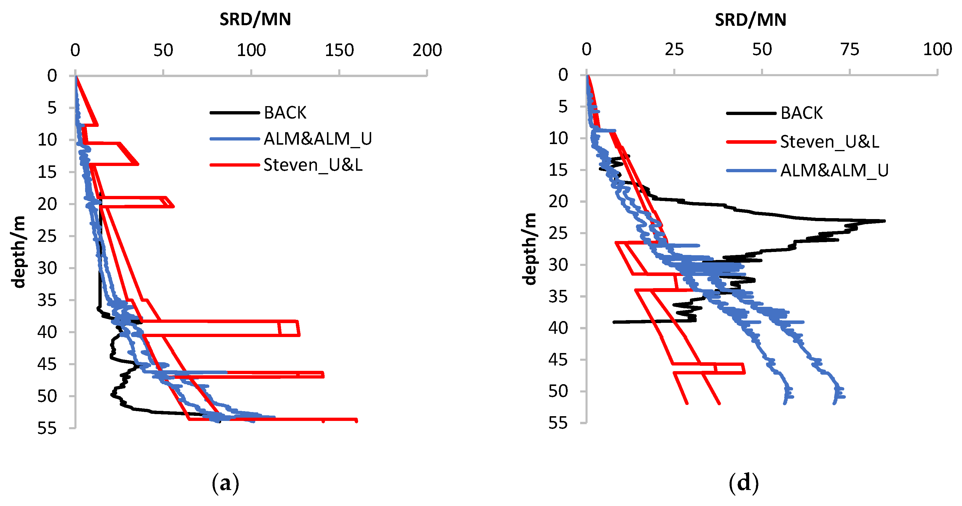
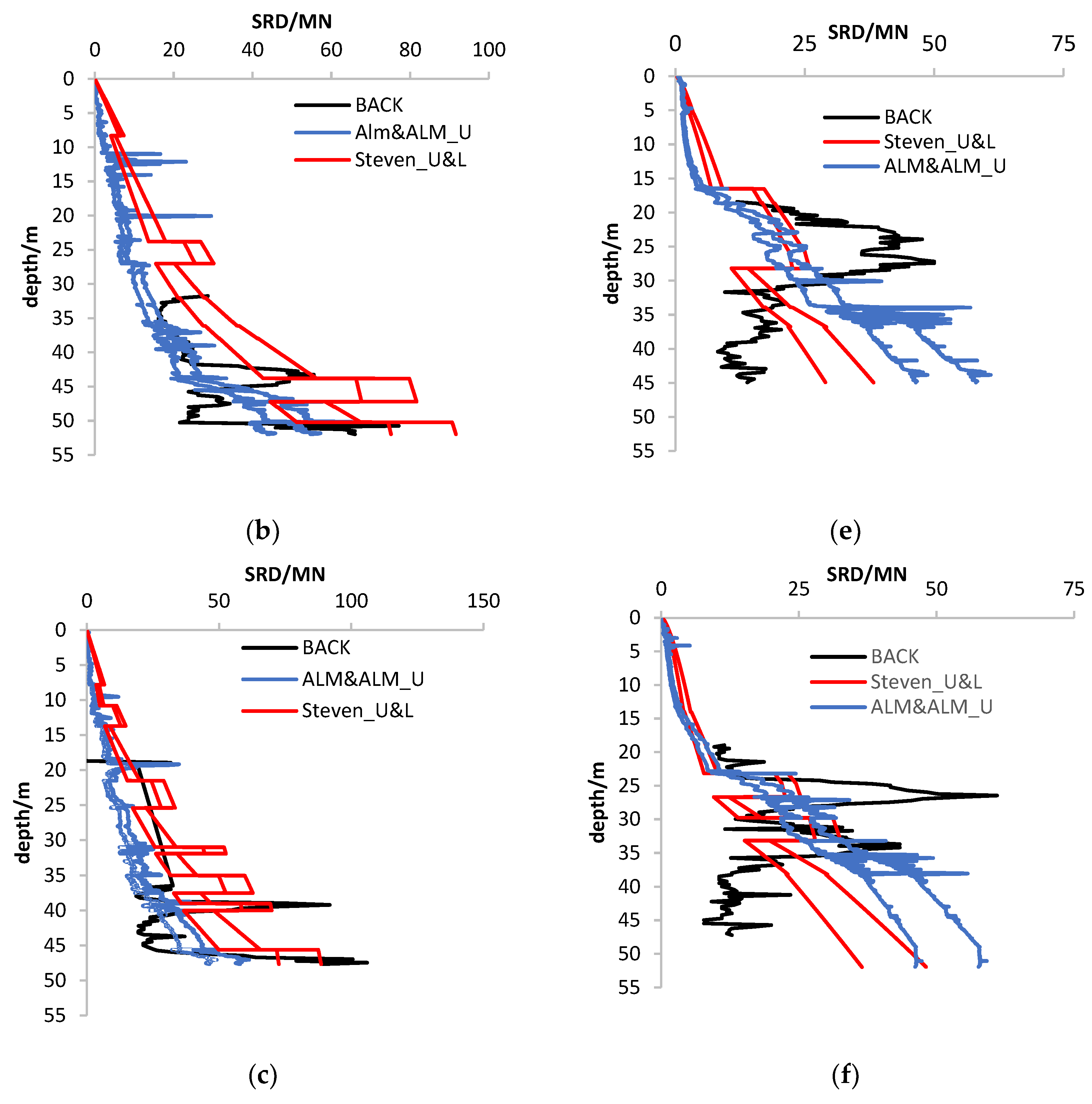
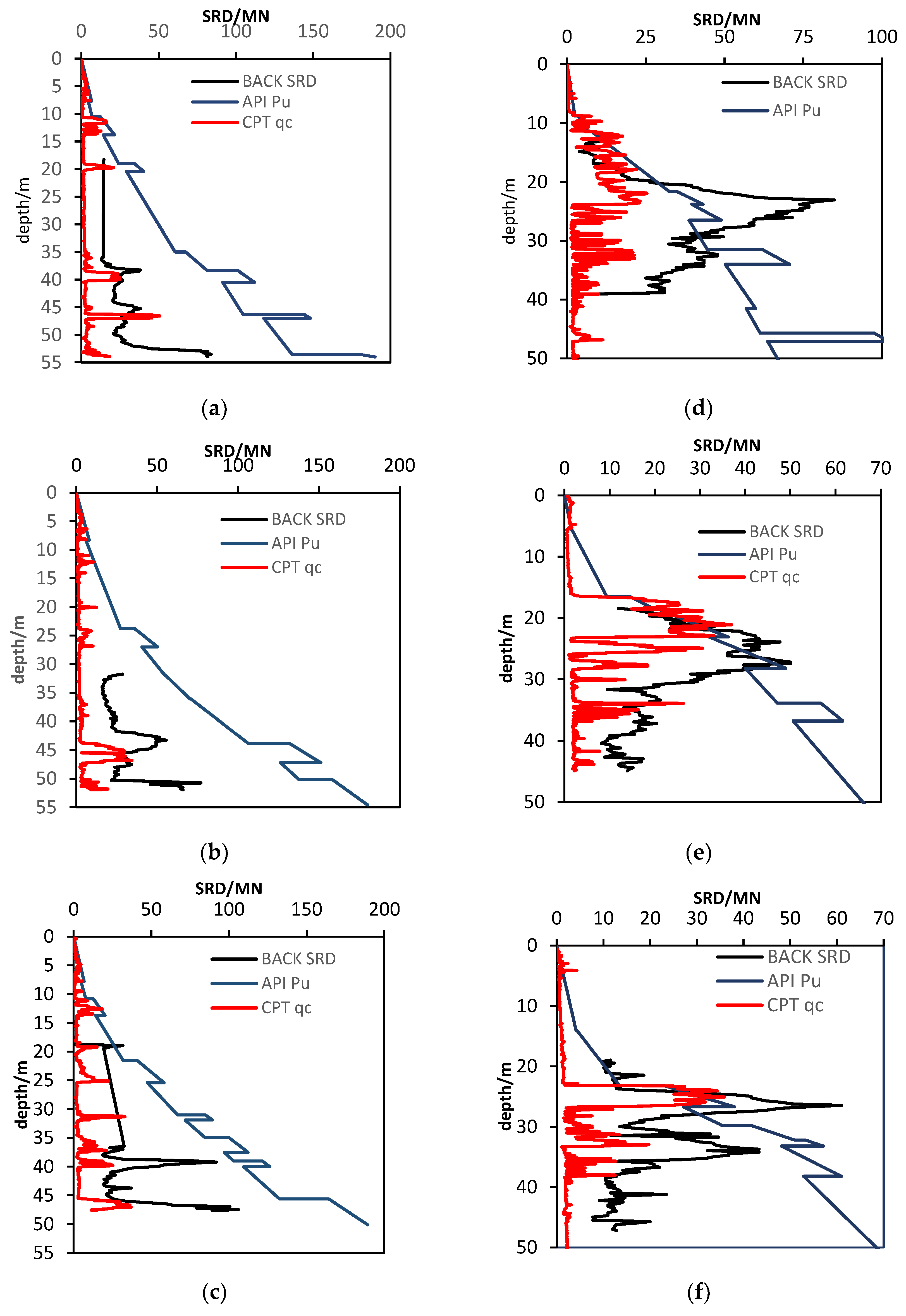
The SRDs calculated using the Steven and Alm methods were generally consistent with those obtained by back analysis based on pile driving records, but the predicted SRD of the clay layer was higher than that obtained by back analysis, while the predicted SRD of sand layer was lower.

(2)

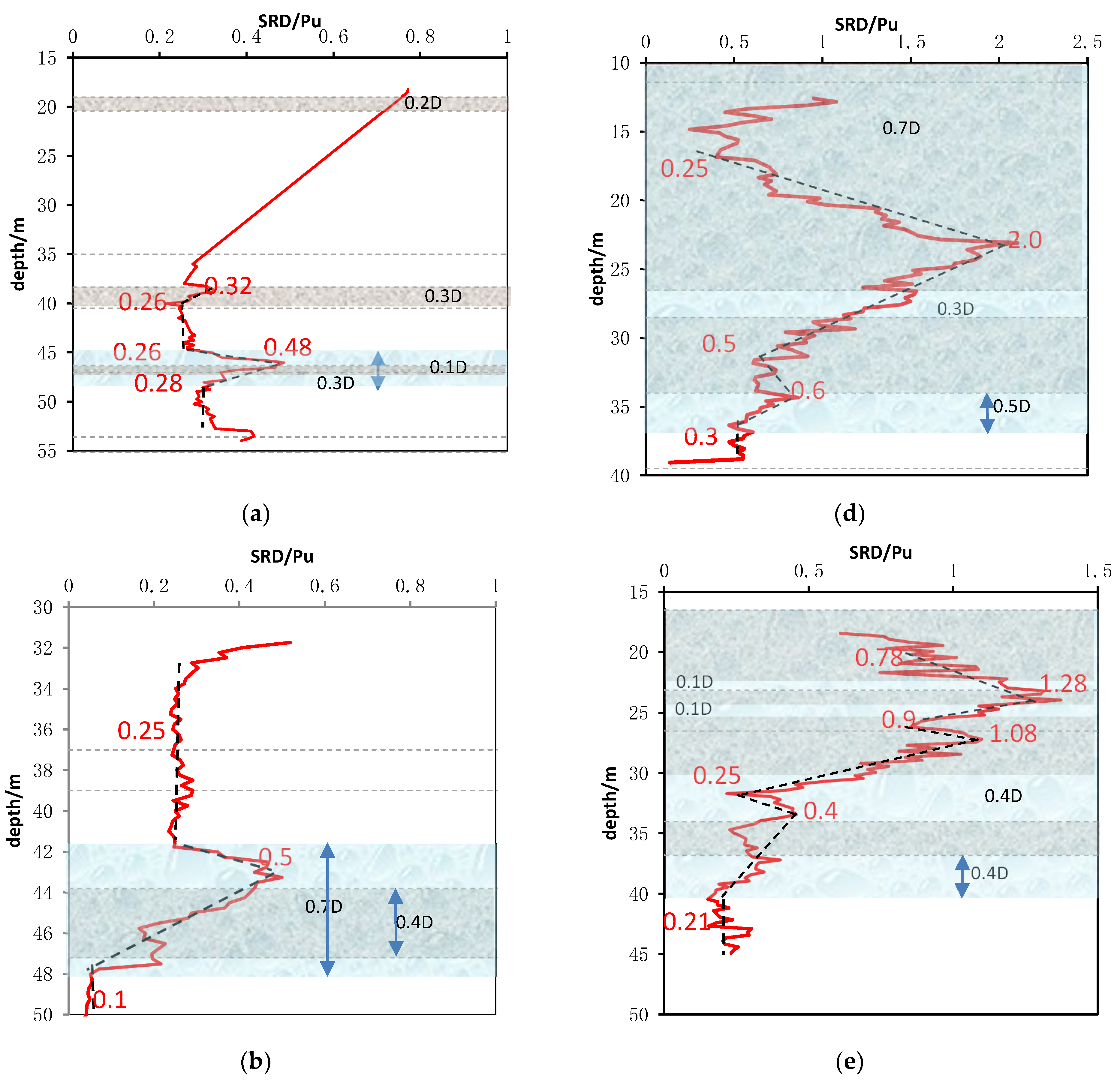
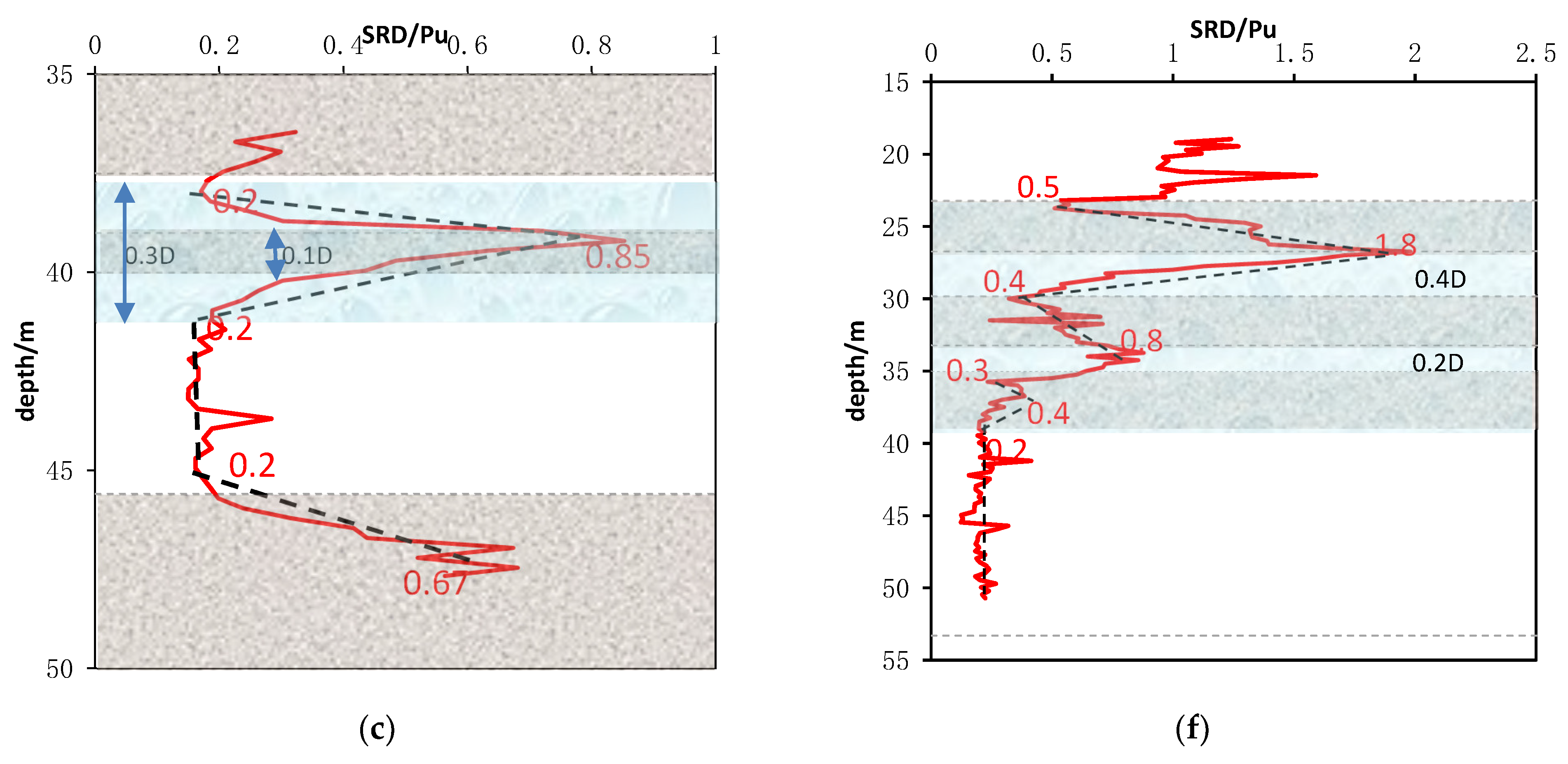
During pile driving, SRD is very sensitive to the presence of a sand layer. Even if the thickness of the sand layer is only 0.1 D, this will cause the obvious fluctuation in SRD in the range of approximately 3 D. The influence of the clay layer with a thickness not exceeding 0.5 D on SRD is mainly concentrated in the range of the clay layer. The SRD/Pu is also sensitive to the presence of a sand layer, while the presence of a clay layer is not significant to SRD/Pu.

(3)

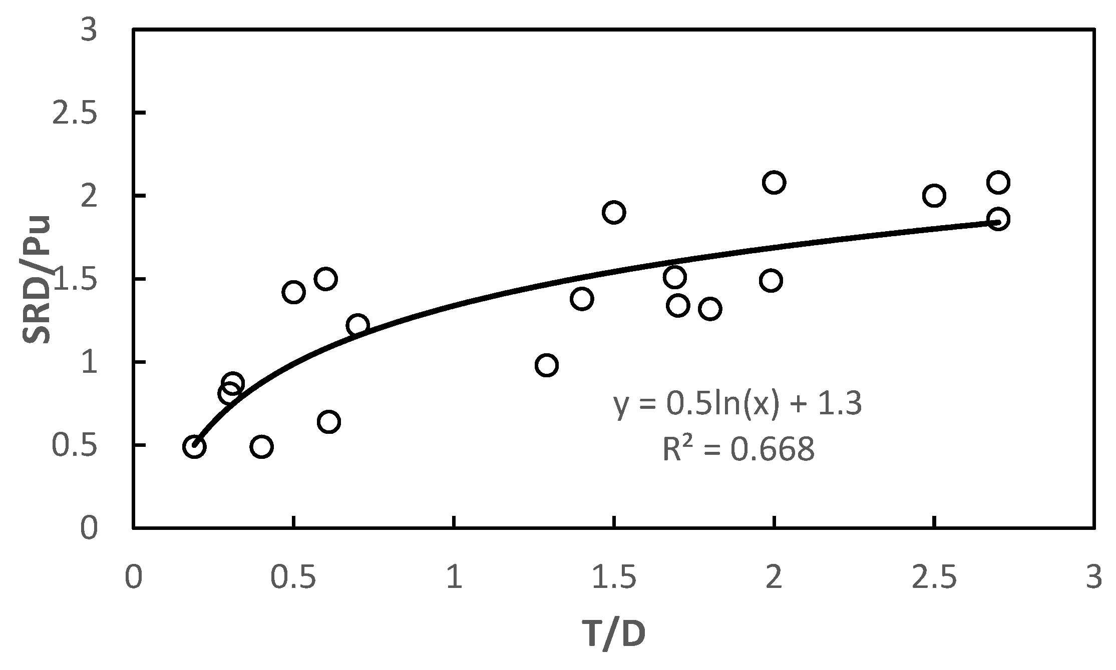
The SRD/Pu for the clay layer is stable, and it is approximately 0.2–0.3 in two kinds of stratified soil regardless of the soil layer distribution. The SRD/Pu of the sand layer shows an approximately linear increment at first and then a decrement with the increase in penetration depth into sand layer, and the maximum SRD/Pu in the sand layer is related to the T/D in this study.

(4)

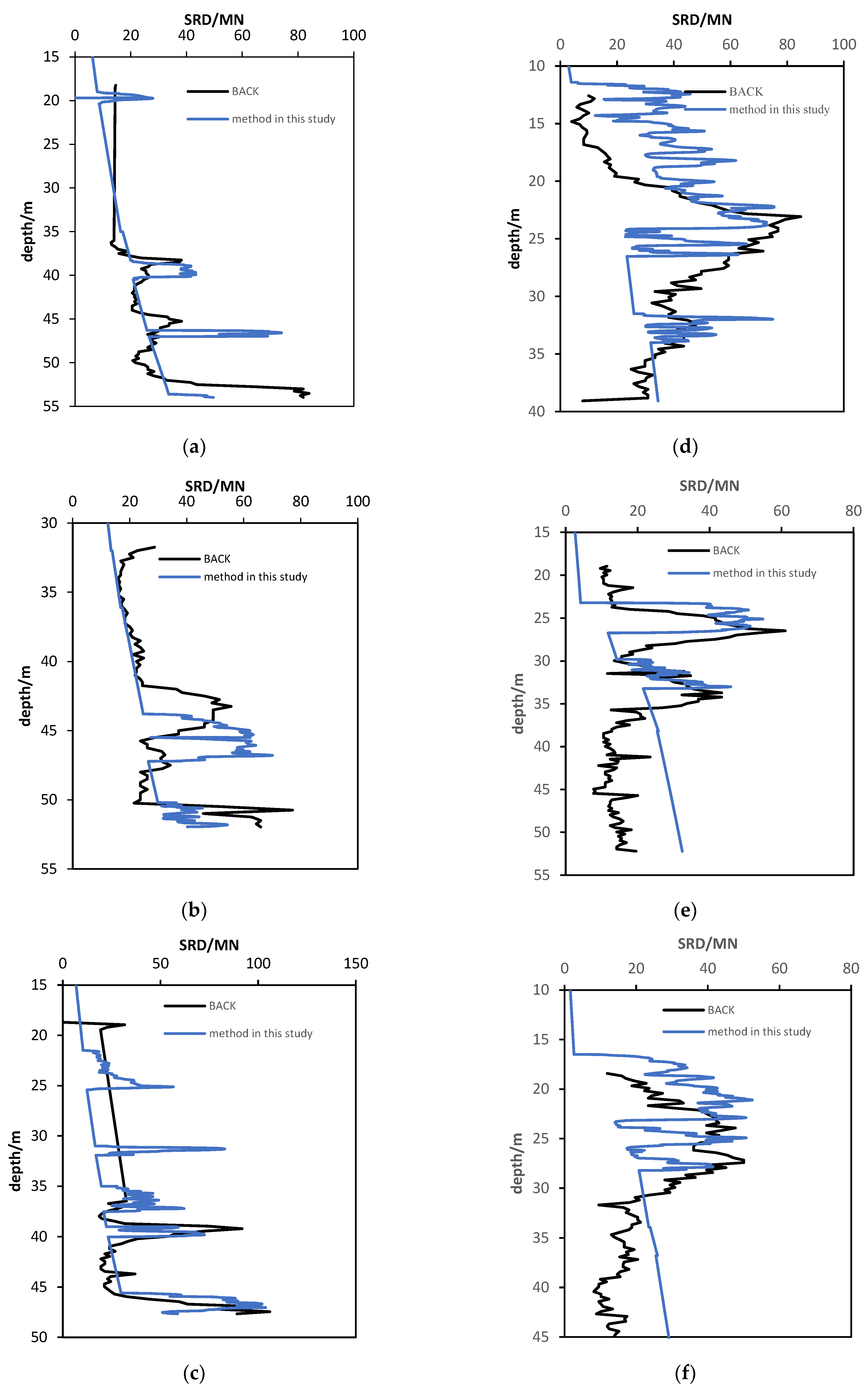
The modified method is proposed by modifying the unit skin friction in clay and the unit end resistance in sand. Considering the influence of the soil layer distribution on the unit end resistance in sand, the reduction factor $\alpha$ is determined considering the influence of T/D. The calculation results show that the proposed method is in good agreement with the results obtained by back analysis.

(5)

In this study, when the thickness of the sand layer is less than or equal to 0. 3 D, pile running occurred. It could be implied that the existence of a thin sand layer is more likely to cause pile running. More attention should be paid to this situation in practice.

Since the relationship between T/D and $\alpha$ is obtained from the pile driving records presented in this study, more data are needed to improve the accuracy of this determination. In addition, because the maximum ratio of SRD/Pu is used to determine the value of $\alpha$ for the sand layer, the SRD calculated by the proposed method could be higher than that in practice.

References

- Zhang, L.; Shi, W.; Zeng, Y.; Michailides, C.; Zheng, S.; Li, Y. Experimental investigation on the hydrodynamic effects of heave plates used in floating offshore wind turbines. Ocean Eng. 2023, 267, 113103. [Google Scholar] [CrossRef]
- Shi, W.; Zhang, L.; Karimirad, M.; Michailides, C.; Jiang, Z.; Li, X. Combined effects of aerodynamic and second-order hydrodynamic loads for three semisubmersible floating wind turbines in different water depths. Appl. Ocean. Res. 2023, 130, 103416. [Google Scholar] [CrossRef]
- Vignesh, V.; Mayakrishnan, M. Design parameters and behavior of helical piles in cohesive soils—A review. Arab. J. Geosci. 2020, 13, 1194. [Google Scholar] [CrossRef]
- Rathod, D.; Krishnanunni, K.T.; Nigitha, D. A Review on Conventional and Innovative Pile System for Offshore Wind Turbines. Geotech. Geol. Eng. 2020, 38, 3385–3402. [Google Scholar] [CrossRef]
- Byrne, B.W.; Houlsby, G. Helical piles: An innovative foundation design option for offshore wind turbines. Philos. Trans. R. Soc. A Math. Phys. Eng. Sci. 2015, 373, 20140081. [Google Scholar] [CrossRef] [PubMed] [Green Version]
- Stanier, S.A.; Black, J.A.; Hird, C.C. Modelling helical screw piles in soft clay and design implications. Geotech. Eng. 2013, 167, 447–460. [Google Scholar] [CrossRef] [Green Version]
- Vignesh, V.; Muthukumar, M. Experimental and numerical study of group effect on the behavior of helical piles in soft clays under uplift and lateral loading. Ocean Eng. 2023, 268, 113500. [Google Scholar] [CrossRef]
- Ding, H.; Wang, L.; Zhang, P.; Liang, Y.; Tian, Y.; Qi, X. The Recycling Torque of a Single-Plate Helical Pile for Offshore Wind Turbines in Dense Sand. Appl. Sci. 2019, 9, 4105. [Google Scholar] [CrossRef] [Green Version]
- Sánchez, S.; López-Gutiérrez, J.-S.; Negro, V.; Esteban, M.D. Foundations in Offshore Wind Farms: Evolution, Characteristics and Range of Use. Analysis of Main Dimensional Parameters in Monopile Foundations. J. Mar. Sci. Eng. 2019, 7, 441. [Google Scholar] [CrossRef] [Green Version]
- Esandi, J.M.; Buldakov, E.; Simons, R.; Stagonas, D. An experimental study on wave forces on a vertical cylinder due to spilling breaking and near-breaking wave groups. Coast. Eng. 2020, 162, 103778. [Google Scholar] [CrossRef]
- Shi, W.; Zeng, X.; Feng, X.; Shao, Y.; Li, X. Numerical study of higher-harmonic wave loads and runup on monopiles with and without ice-breaking cones based on a phase-inversion method. Ocean Eng. 2023, 267, 113221. [Google Scholar] [CrossRef]
- Webster, S.; Robinson, B. Driveability Analysis Techniques for Offshore Pile Installations. In Proceedings of the ASME 2013 32nd International Conference on Ocean, Offshore and Arctic Engineering, Nantes, France, 9–14 June 2013. [Google Scholar] [CrossRef] [Green Version]
- Lehane, B.M.; Randolph, M.F. Evaluation of a Minimum Base Resistance for Driven Pipe Piles in Siliceous Sand. J. Geotech. Geoenviron. Eng. 2002, 128, 198–205. [Google Scholar] [CrossRef]
- Smith, E.A.L. 1960, Pile Driving Analysis by the Wave Equation. J. Soil Mech. Found. Div. 1962, 127, 1145–1193. [Google Scholar]
- Semple, R.M.; Gemeinhardt, J.P. Stress history approach to analysis of soil resistance to pile driving. In Proceedings of the Offshore Technology Conference, Houston, TX, USA, 1–4 May 1981. [Google Scholar] [CrossRef]
- Stevens, R.S.; Wiltsie, E.A.; Turton, T.H. Evaluating pile drivability for hard clay, very dense sand, and rock. In Proceedings of the Offshore Technology Conference, Houston, TX, USA, 3–6 May 1982. [Google Scholar] [CrossRef]
- Toolan, F.E.; Fox, D.A. Geotechnical planning of piled foundations for offshore platforms. Proc. Inst. Civ. Eng. 1977, 62, 221–244. [Google Scholar] [CrossRef] [Green Version]
- Alm, T.; Hamre, L. Soil model for pile driveability predictions based on cpt interpretations. In Proceedings of the International Conference on Soil Mechanics and Geotechnical Engineering, Istanbul, Turkey, 27–31 August 2001. [Google Scholar]
- Schneider, J.A.; Harmon, I.A. Analyzing drivability of open ended piles in very dense sands. DFI J.—J. Deep Found. Inst. 2010, 4, 32–44. [Google Scholar] [CrossRef]
- Jardine, R.J.; Chow, F.C.; Overy, R.F.; Standing, J. ICP Design Methods for Driven Piles in Sands and Clays; Institution of Civil Engineering (ICE): London, UK, 2005. [Google Scholar]
- Lehane, B.; Schneider, J.; Xu, X. The UWA-05 method for prediction of axial capacity of driven piles in sand. In Proceedings of the International Symposium on Frontiers in Offshore Geotechnics, Perth, Australia, 19–21 September 2005. [Google Scholar]
- Kolk, H.J.; Baaijens, A.E.; Senders, M. Design criteria for pipe piles in silica sands. In Proceedings of the First International Symposium on Frontiers in Offshore Geotechnics, Perth, Australia, 19–21 September 2005. [Google Scholar]
- Prendergast, L.J.; Gandina, P.; Gavin, K. Factors influencing the prediction of pile driveability using cpt-based approaches. Energies 2020, 13, 3128. [Google Scholar] [CrossRef]
- Anusic, I.; Eiksund, G.; Liingaard, M. Comparison of pile driveability methods based on a case study from an offshore wind farm in North Sea. In Proceedings of the 17th Nordic Geotechnical Meeting Challenges in Nordic Geotechnic, Reykjavik, Iceland, 25–28 May 2016; pp. 1037–1046. [Google Scholar]
- Available online: https://www.bladt.dk/ (accessed on 1 October 2022).
- Ferreira, J.M. Drveability Study for XL Offshore Monopile Foundation. Master’s Thesis, University of Porto, Porto, Portugal, 2016. [Google Scholar]
- Davidson, J.; Castelletti, M.; Torres, I.; Terente, V.A.; Irvine, J.; Raymackers, S. The evaluation of current pile driving prediction methods for driven monopile foundations in London clay. In Proceedings of the 20th International Conference on Soil Mechanics and Geotechnical Engineering, Paris, France, 19–20 February 2018. [Google Scholar]
- Byrne, T.; Gavin, K.; Prendergast, L.J.; Cachim, P.; Doherty, P.; Chenicheri Pulukul, S. Performance of CPT-based methods to assess monopile driveability in north sea sands. Ocean Eng. 2018, 166, 76–91. [Google Scholar] [CrossRef] [Green Version]
- Georgios, P.S.; Meissl, T.S. Evaluation of SRD methodologies prediction accuracy at offshore wind farms in the Irish Sea. In Proceedings of the 16th Asian Regional Conference on Soil Mechanics and Geotechnical Engineering, Taipei, Taiwan, 14–18 October 2019. [Google Scholar]
- Maynard, A.W.; Hamre, L.; Butterworth, D.; Davison, F. Improved Pile Installation Predictions for Monopiles, Stress Wave Theory and Testing Methods for Deep Foundations: 10th International Conference; ASTM International: West Conshohocken, PA, USA, 2019; pp. 426–449. [Google Scholar] [CrossRef]
- Jamiolkowski, M.; Ghionna, V.N.; Lancellotta, R.; Pasqualini, E. New correlations of penetration tests for design practice. In Penetration Testing 1988: Proceedings of the First International Symposium on Penetration Testing ISOPT-1, Orlando, FL, USA, 20–24 March 1988; Pergamon: Oxford, UK, 1990. [Google Scholar]
- Robertson, P.K.; Cabal, K. Guide to Cone Penetration Testing; Gregg Drilling LLC.: California, CA, USA, 2022. [Google Scholar]
- Lambe, T.W.; Whitman, R.V. Soil Mechanics; John Wiley & Sons: California, CA, USA, 1969. [Google Scholar]
- Lunne, T.; Robertson, P.K.; Powell, J.J.M. Cone Penetration Testing in Geotechnical Practice; Blackie Academic & Professional: London, UK, 1997. [Google Scholar]
- De Ruiter, J.; Beringen, F.L. Pile foundations for large North Sea structures. Mar. Geotechnol. 1979, 3, 267–314. [Google Scholar] [CrossRef]
- Bustamante, M.; Gianeselli, L. Pile bearing capacity by means of static penetrometer CPT. In Proceedings of the 2nd European Symposium on Penetration Testing, Amsterdam, The Netherlands, 24–27 May 1982. [Google Scholar]
- White, D.J.; Bolton, M.D. Comparing CPT and pile base resistance in sand. Geotech. Eng. 2005, 158, 3–14. [Google Scholar] [CrossRef]
- Randolph, M.F.; May, M.; Leong, E.C.; Hyden, A.M.; Murff, J.D. Soli plug response in open ended pipe piles. J. Geotech. Eng. 1992, 118, 743–759. [Google Scholar] [CrossRef]