Article

Insight into Hydrodynamic Damping of a Segmented Barge Using Numerical Free-Decay Tests

1
Faculty of Electrical Engineering, Mechanical Engineering and Naval Architecture, University of Split, R. Boškovića 32, 21000 Split, Croatia
2
Faculty of Mechanical Engineering and Naval Architecture, University of Zagreb, Ivana Lucica 5, 10000 Zagreb, Croatia
3
Bureau Veritas, Research Department, 67/71 Boulevard du Château, 92200 Neuilly-sur-Seine, France
*
Author to whom correspondence should be addressed.
J. Mar. Sci. Eng. 2023, 11(3), 581; https://doi.org/10.3390/jmse11030581
Submission received: 17 February 2023 / Revised: 3 March 2023 / Accepted: 6 March 2023 / Published: 8 March 2023
(This article belongs to the Special Issue CFD Applications in Ship and Offshore Hydrodynamics)

Abstract

:
Natural vibrations of a segmented and a monohull barge are analysed to compare influences of hydrodynamic damping on the dynamic responses of two different models. The influence of water flow around and between barge segments on hydrodynamic damping was investigated by simulating free-decay tests using a URANS method. Fluid forces were fed into the modal solver, which allows for efficient deformation of the structure without full resolution of structural equations. Verification of the coupled solver was performed by reproducing the model experiments of a segmented barge. Comparison of segmented and monohull results clarified the impact of gaps between barge segments, i.e., how the energy dissipates because of large pressure gradients within and around gaps, and additional free-surface movement. This insight of higher damping should be taken into account for model tests of segmented floating structures, such as wave-energy-converting systems.

1. Introduction

In unsuitable environmental conditions, i.e., sea state, heading and speed, highly nonlinear loads occur on the ship’s hull and cause significant vibrations and noise, which are transmitted along the hull’s structure [1]. In rough seas, the ship’s bow and stern may occasionally emerge from a wave and re-enter the wave with a heavy impact or a slam [2] as the hull structure encounters the water, developing high hydrodynamic loads that produce significant vibrations. Ship-hull vibration is a major contributor to fatigue-crack growth [3,4], and structural vibrations radiate noise [5]. It is of importance to determine the vibration level of a ship in the design stage. This urgency is caused by the increasing propulsion power and very large sizes of ships. The damping is the dissipation of the energy during a vibration cycle, and it is a key parameter in resonance phenomena that influences the amplitude of harmonic vibrations and the number of significant vibration cycles in the case of transient vibrations, for example. The damping in lightly damped vibrations can be overlooked in the determination of the system’s natural frequencies, but it will have a large effect on the vibration response around the natural frequencies; i.e., the excitation at resonance is only equilibrated by damping. The damping of structural systems and ships in particular is weak. Except when extremely close to resonance, the vibratory amplitude is approximately independent of damping [6]. The total damping associated with overall ship hull vibration is generally considered to be a combination of the structural damping (e.g., steel hysteresis effects), cargo damping (e.g., cargoes of grain) and hydrodynamic damping (viscous and wave damping). Hydrodynamic damping is frequency-dependent and approaches zero for high and very low frequencies. Viscous hydrodynamic damping is often nonlinear and caused by bilge keels, skin friction, vortices, etc. Water impacts that occur on the flat stern as a consequence of violent vibration may actually contribute as a nonlinear damping due to antisymmetric loading [7]. In general, the effect of wave creation is disregarded, but it must be considered for vibrations with low frequencies [8]. Typically, an overall constant damping coefficient of around 1.5% of the critical damping is employed as a preliminary estimate [9,10].
In this study, the hydroelastic response of a floating object was simulated numerically by coupling two solvers: a fluid dynamics solver and a structural solver. In the literature, different kinds of methodologies have been established for the two-way fluid–structure interaction (FSI). Fully coupled (monolithic) techniques incorporate both the fluid and the structure equations, while relying on a single solver for the coupled system [11]. Classical CFD solutions are constructed mostly on Eulerian reference systems, thereby connecting the structural equations based on the Lagrangian reference system results in the matrices for structure systems more rigid than those for fluid systems. Solving equations using a unified method for large-scale problems is therefore computationally intensive. Using two independent solvers, partitioned methods solve the structure and fluid equations on two separate grids. In order to map the surface loads from the CFD grid to the structure grid and the displacement field from the structure grid to the CFD grid, a communication method must be established at the interface between the grids [12]. Displacement of the CFD grid’s boundary necessitates careful manipulation of the surrounding nodes without tangling or twisting the cells or remeshing the deformed region. There have been successful attempts at using partitioned methods by coupling them with potential flow theory [13,14,15], directly coupling structure solvers with the CFD solver [16,17] and by using the boundary-integral equation method [18].
In this paper, weak coupling of the unsteady RANS-VOF solver with the reduced-order modal approach is considered, which enables rapid simulation of flexible floating structures for known vibration-mode shapes and their natural frequencies [19] that can be obtained by analytical, experimental, or numerical analysis. Fast, unsteady simulation in the time domain can give an insight into the structural response to any kind of external loads. The coupling was established in FineMarine CFD software based on modal simulations performed using NASTRAN solver. We focus on the determination of the hydrodynamic damping in the case of a flexible barge that is vertically freely vibrating, based on an extensively documented experiment [20] that was rendered in Figure 1. In comparison to realistic monohull ship models, the modal damping ratios for this segmented vibrating structure were found to be unusually high in comparison to regular floating structures. This phenomenon is caused by the influence of the barge gaps on the hydrodynamics. Therefore, numerical simulations were performed for the segmented structure and the monohull structure in order to clarify the impact of the gaps between pontoons on the hydrodynamic response of the floating structure. A CFD approach was used that was similar to those applied in [16,21]. The aims of the investigation were twofold: to show that weak coupling of a validated RANS solver and stable modal solver is quick and accurate, and to analyse the hydrodynamic damping generated by segmented sections of vibrating floating structures.
The paper is organised as follows. In the next section, the flow and structure of the numerical solvers are described. In Section 3, the coupling between the solvers is introduced. Section 4 describes the numerical experiment and numerical results. The last section presents an explanation of the results and the conclusions.

2. Numerical Methods

2.1. Modal Solver for the Structure

The equation of motion for a multiple-degree-of-freedom (MDOF) system is written as:
M x ¨ t + C x ˙ t + K x t = f t
where x t , x ˙ t and x ¨ t are, respectively, vectors of displacement, velocity and the acceleration responses of the system induced by the time-dependent external force vector f t ; and M , C and K are mass, damping and stiffness matrices, respectively. The addition of damping terms in slightly damped vibration systems may be neglected in the determination of the natural frequencies of the system. Considering the free motion, real mode shapes are the solution to the eigenvalue problem:
K ω 2 M Φ = 0
where Φ is the modal matrix that consists of mode shape vectors for each natural frequency of the system with n degrees of freedom: Φ = ϕ 1 , ϕ 2 , , ϕ n . A mode shape describes the form of the vibration for a particular natural frequency ω i . The non-trivial solution of eigenvalue problem (2) exists when:
det K ω 2 M = 0 .
The solution of Equation (3) is the vector of squared values of the system’s natural frequencies, ω 1 2 , ω 2 2 , , ω n 2 . The obtained eigenvectors of an undampened system are orthogonal to each other, such that ϕ i T M ϕ j = ϕ i T K ϕ j = 0 holds for any i and j modes of vibration, i j . From the orthogonality properties, it holds that the modal mass matrix, Φ T M Φ , and the modal stiffness matrix, Φ T K Φ , are diagonal matrices with the modal quantities on their diagonals. Since the absolute magnitude of a mode shape is not definite, eigenvectors are usually normalised with respect to the system’s mass:
Φ ˜ T M Φ ˜ = I
where Φ ˜ is the mass-normalised modal matrix and  I is the identity matrix. From Equation (2), it follows that
Φ ˜ T K Φ ˜ = diag ω 1 2 , ω 2 2 , , ω n 2 .
The global deformation of the structure can be written as a superposition of the vibration modes:
x t = Φ ˜ u t
where u t is the vector of modal coordinates (or the generalised displacement). Using the modal coordinate transformation (6) and mass-normalised modal matrix, Φ ˜ , the equation of motion (1) can be expressed as:
Φ ˜ T M Φ ˜ u ¨ t + Φ ˜ T C Φ ˜ u ˙ t + Φ ˜ T K Φ ˜ u t = Φ ˜ T f t
where u ˙ t and u ¨ t are vectors of modal velocity and the modal acceleration response of the system, respectively. The convenient outcome is that all terms in Equation (7) are diagonal matrices, except the damping term, Φ ˜ T C Φ ˜ .

2.2. Rayleigh Damping

In order to uncouple the equation of motion of a MDOF system into n equations of motion of a single degree-of-freedom (SDOF) system, the damping term should also be diagonalised. Lord Rayleigh introduced the damping matrix, which is assumed to be proportional to the mass and stiffness matrices:
C = α M + β K
where α and β are the mass and stiffness coefficients, respectively. There are no physical reasons for the damping matrix to have this kind of relation with the other matrices, but it offers the advantage of diagonalising the equation of motion for the real mode shapes. By inserting the damping matrix (8) into the transformed equation of motion (7), and by using the relations (4) and (5), n uncoupled SDOF equations may be written as:
u i ¨ t + α + β ω i 2 u i ˙ t + ω i 2 u i t = ϕ i T f t .
Equation (9) can conveniently be expressed as:
u i ¨ t + 2 ζ i ω i u i ˙ t + ω i 2 u i t = ϕ i T f t
where ζ i is the modal damping ratio of mode i. This ratio expresses the level of actual damping in a system relative to critical damping, ζ i = c i / c c , where the critical damping coefficient is defined as c c = 2 m ω i .
The solution to Equation (10) can be obtained for each vibration mode by using direct integration algorithm, e.g., the Newmark integration method or the complementary function and a particular solution method [19].

2.3. Damping Determination

The logarithmic decrement method is used to find the damping ratio of an under-damped system in the time domain. The method relies on the natural logarithm of the ratio of two successive peaks amplitudes:
δ = ln x t x t + T
where t is time when the amplitude is reached and T is the period of vibration. The damping ratio is then found from the following expression:
ζ i = 1 1 + 2 π δ 2
In addition to the amplitudes, the logarithmic decrement may be calculated using acceleration amplitudes, x ¨ t and x ¨ t + T , if the response is purely single-mode like it is considered to be later in the paper. The above logarithmic decrement method is used to determine the damping ratio based on the numerically obtained structure response.

2.4. Flow Solver

The Navier–Stokes equation that describes conservation of momentum of fluid flow, for the incompressible viscous fluid, reads:
D v D t = 1 ρ p + μ ρ 2 v + 1 ρ a e x t
and the equation of continuity that describes the conservation of mass, i.e., the incompressibility constraint, reads:
· v = 0
where v is the velocity vector field, D / D t denotes material derivative / t + v · , p is the pressure field, ρ is the fluid density, μ is the dynamic viscosity of the fluid and  a e x t denotes external forces acting on fluid (e.g., gravity acceleration). FineMarine CFD software was utilised to model and numerically analyse the flows surrounding the barge. For spatial discretisation of the transport equations, the finite volume method (FVM) was applied. The solver uses incompressible unsteady RANS equations and the VOF approach for free-surface capturing. The pressure equation is solved on the faces of an unstructured three-dimensional mesh whose cells are connected by an arbitrary number of faces. Menter’s K– ω turbulent shear stress model was used to capture flow separation. The flow domain extends two barge lengths around the model. The no-slip boundary condition is imposed on the hull by using wall functions. The far-field boundary condition is imposed at the front, back and side boundaries of the domain, where the flow enters or leaves the domain locally. The pressure is specified as a Dirichlet boundary condition at the top and bottom boundaries of the domain. The flow solver has been thoroughly validated [22,23,24].

3. Modal-Based Coupling

In this paper, we investigate the weakly coupled FSI using a reduced-order model for the structure because this type of model is more computationally efficient than direct models [19]. Reduced-order models are useful when one has to deal with complex structures, such as ships, whose dynamics are governed by well defined modes of vibration. As discussed in Section 2.1, a vibrating structure can be represented by mass-normalised mode shapes and natural frequencies. The right-hand-side of Equation (1) or (10) is the force vector, which is directly responsible for linking the unsteady hydrodynamics and inertial loads with the structural system. The modal, Equation (10), can therefore be solved externally or even directly inside the fluid flow solver at each physical time step, for all known mode shapes. The global deformation of the structure is reconstructed with Equation (6), which is often termed as mode superposition, in order to take the new shape of the structure into account for the flow calculation. Therefore, for the partitioned fluid–structure interaction, the external loads are applied by the fluid flow, but the fluid flow is also influenced by the deformation of the structure.
Prior to the CFD simulation, the structure’s dry natural frequencies and mode shapes were calculated outside of the flow solver. Vibrating mode shapes are represented using generalised displacements, i.e., vectors of modal coordinates relative to the initial structure shape that can be obtained analytically, numerically or experimentally.
Structure and fluid solvers have to exchange forces and displacements, and the structure and fluid interface are differently discretised. A robust way to interpolate values and deform CFD mesh around deforming structures is the radial basis function (RBF) interpolation [25]. A fluid volume mesh has to be deformed at each time step according to the displacements obtained by the modal solver at the interface of the fluid–structure domain. By using RBF, the fluid grid is smoothly deformed by interpolating the displacements of the boundary nodes to all the volume mesh nodes. The system of equations that involves only boundary nodes has to be solved and does not have the need for grid topology information. Therefore, dry mode shapes can be represented with an arbitrary number of generalised displacements at the solid–fluid interface, while taking into account limitations of RBF (e.g., all points should not lie on a single line). Increasing the number of structural nodes (and displacements) increases the size of the transformation matrix and memory requirements, but increases the accuracy of fluid–structure loads and displacements transfer. In order to accelerate inter-grid communication, it advisable to generate connections between fluid boundary grid nodes and structural nodes based on RBF interpolation before running the simulation.
The steps of computational method are shown in Algorithm 1. The equilibrium between the structure and the fluid is not exactly ensured at the end of each solver iteration, i.e., each time step, which is referred to as the weak coupling. The structure solver is second-order time-accurate, and the fluid solver verifying the conservation laws is at least first-order time accurate; thus, the computational method is at least first-order time accurate.
Algorithm 1 Reduced order modal approach to weakly coupled FSI.
1. Calculate dry vibration natural frequencies ω 1 , ω 2 , , ω n and their mass-normalised mode shapes
2. Setup simulation initial conditions (e.g., initial structure displacement and fluid boundary conditions)
3. Build RBF connections fluid face/structural node
4. Simulation loop, for each time-step Δ t :
 (a) Transfer fluid loads to structural nodes
 (b) Solve set of Equation (10) for all mode shapes
 (c) Obtain new shape of the structure via Equation (6)
 (d) Perform RBF mesh interpolation from the old to the new structure shape
 (e) Solve flow for time t + Δ t , influenced by the deformation of the structure
 (f) If residuals of fluid solver are too high, go to step 4.(a)

4. Vertical Vibrations of a Flexible Barge

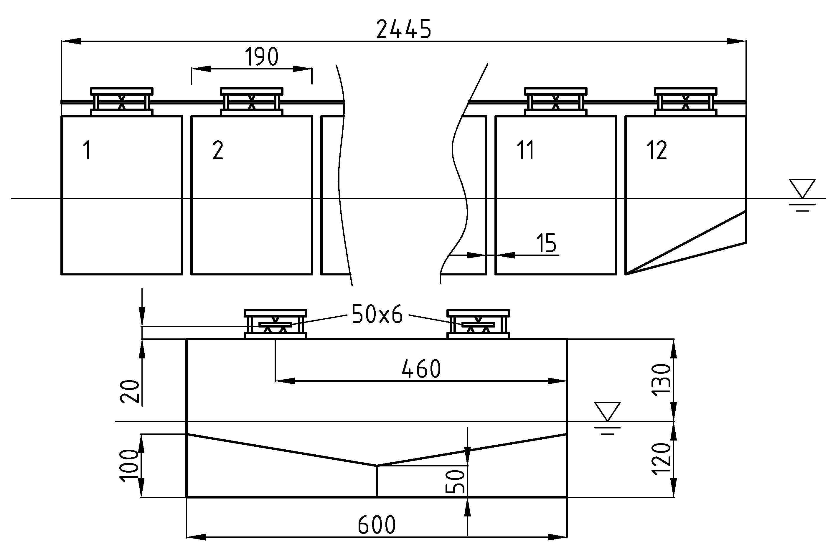
4.1. Barge Characteristics

Numerical experiments were performed on a flexible barge, based on experimental setup from [20]. The experiments which were used in the present work are quite particular, and they are not intended for realistic model ship models. The initial purpose of these experiments was to validate the numerical developments related to global hydroelastic aspects. For that reason, the elasticity of the plates was chosen in such a way that the resonant frequencies got close to the wave frequencies which can be realised in the basin. This was practically possible to achieve only with the segments disconnected from each other, i.e., with gaps included.
The experimental model of a flexible prismatic barge consisted of twelve segments or pontoons (that had the following dimensions: length 190 mm, breadth 600 mm, depth 250 mm). The pontoons were shaped as rectangular boxes, except for the foremost one, which had a slightly modified keel, which is visible in Figure 1 and Figure 2. Two elastic steel plates were positioned above the deck level and were connected to the pontoons, as shown in Figure 1. Each plate had the following dimensions: width 50 mm, height 6 mm. The draught of the barge was 120 mm, and the pontoons were separated by 15 mm gaps, in order to avoid contact while vibrating.
In order to extract wet natural frequencies and damping ratios from the experimental model, a modal analysis was performed on the data obtained from series of free decay tests. The tests were initiated by releasing the barge pulled by the first floater out of the water in the vertical direction. The data obtained from the experiment are vertical displacements yielded from six optical sensors placed on the tops of the pontoons. Yielded natural frequencies and average damping ratios for the first two vibration modes are given in Table 1. The modal damping ratios in these cases are unusually high in comparison to regular floating structures. It is rational to assume that this phenomenon is caused by the influence of the barge gaps on the hydrodynamics, so this particular problem qualifies the experiment as a good verification test for a numerical hydroelastic solver. Furthermore, numerical simulations were also performed on the monohull structure without the gaps in order to clarify the impact of the gaps between pontoons on the hydrodynamic response of the floating structure.

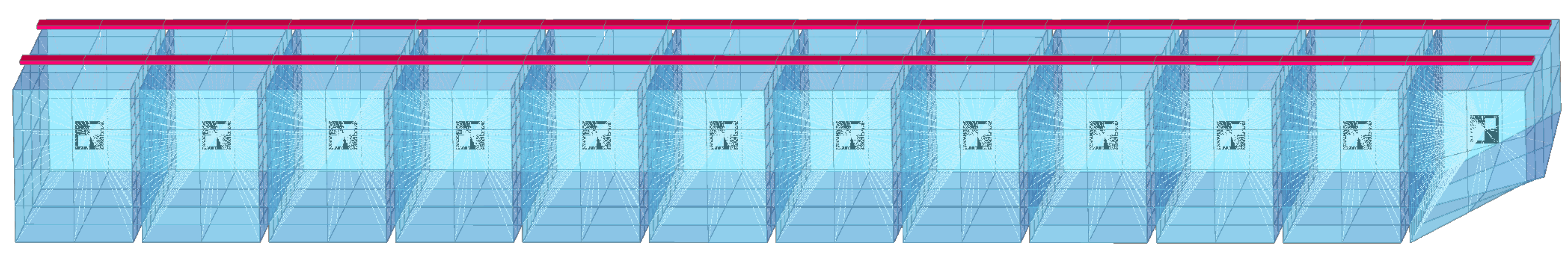
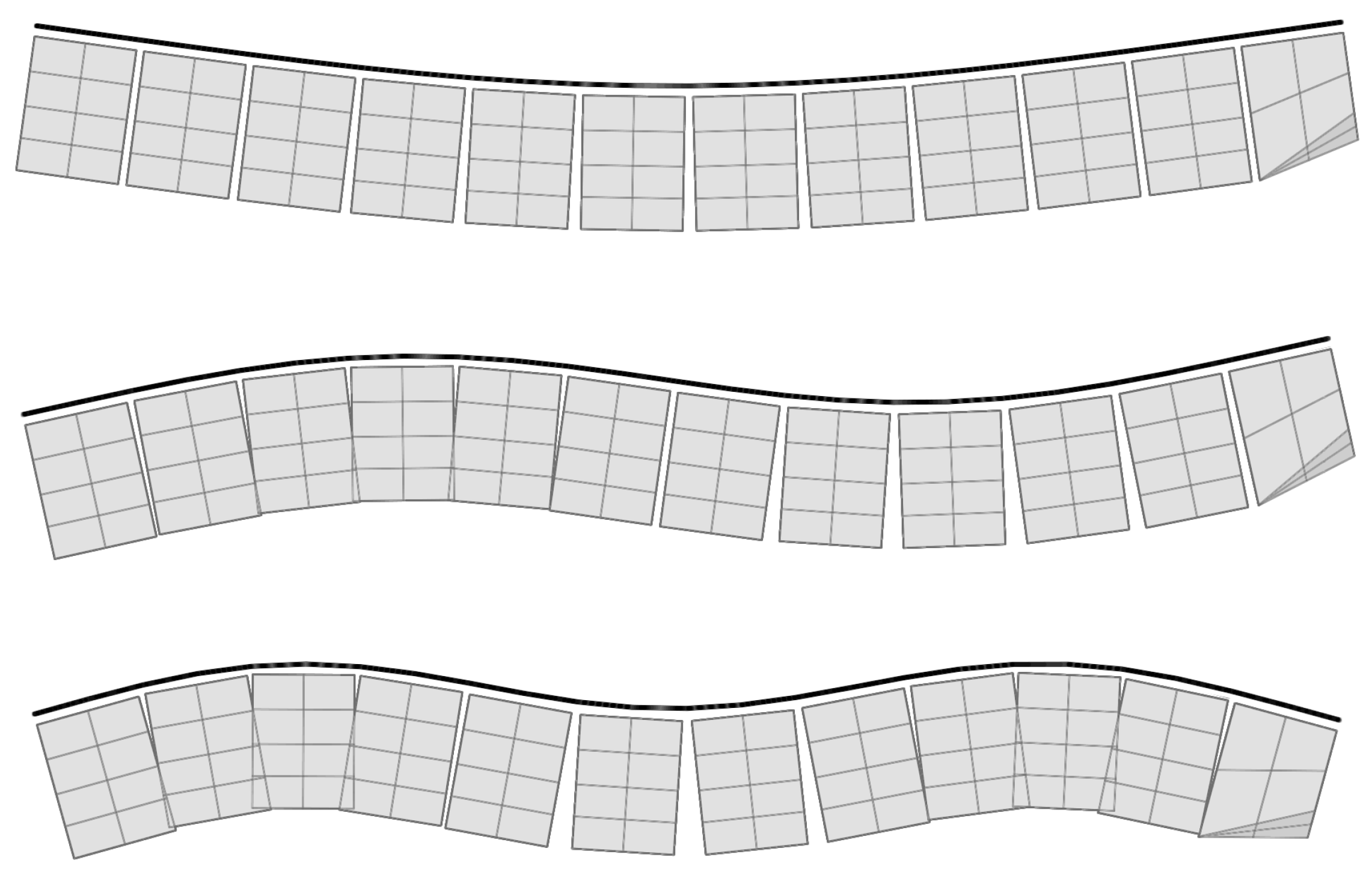
4.2. Extraction of Mode Shapes

Natural vibration analysis was performed by using the NASTRAN solver on a finite element (FE) structural model, which was constructed using beam elements that were rigidly connected to the pontoons. Massless and infinitely stiff shells of pontoons were constructed to act as an interface between the structural and fluid model for the hydroelastic analysis. The FE model is shown in Figure 2. The first three mode shapes we obtained of the vertically vibrating barge are rendered in Figure 3. The mode shapes agree with the experimental modal analysis, and they correspond to analytic-mode shapes of a vertically vibrating free-form beam with a constant cross-section.
Since the dry natural frequencies are not known from experimental analysis, the dry natural frequencies obtained using the finite element analysis (FEA) were compared with the analytically obtained results using Timoshenko’s theory for beams with uniform cross-sections [1], and the results are presented in Table 2. To validate the beam model by comparing it to Timoshenko’s theory for beams, FEA was performed on pontoon masses that were temporary brought upwards to the level of the beam axis. The natural frequencies obtained in this scenario match the analytically obtained values. It can be seen that the natural frequencies obtained numerically through the model with a proper mass distribution, as shown in Figure 2, are somewhat lower than the analytically obtained values. This was expected, due to the emphasised influence of the rotational inertia of heavy pontoons attached to the beams.

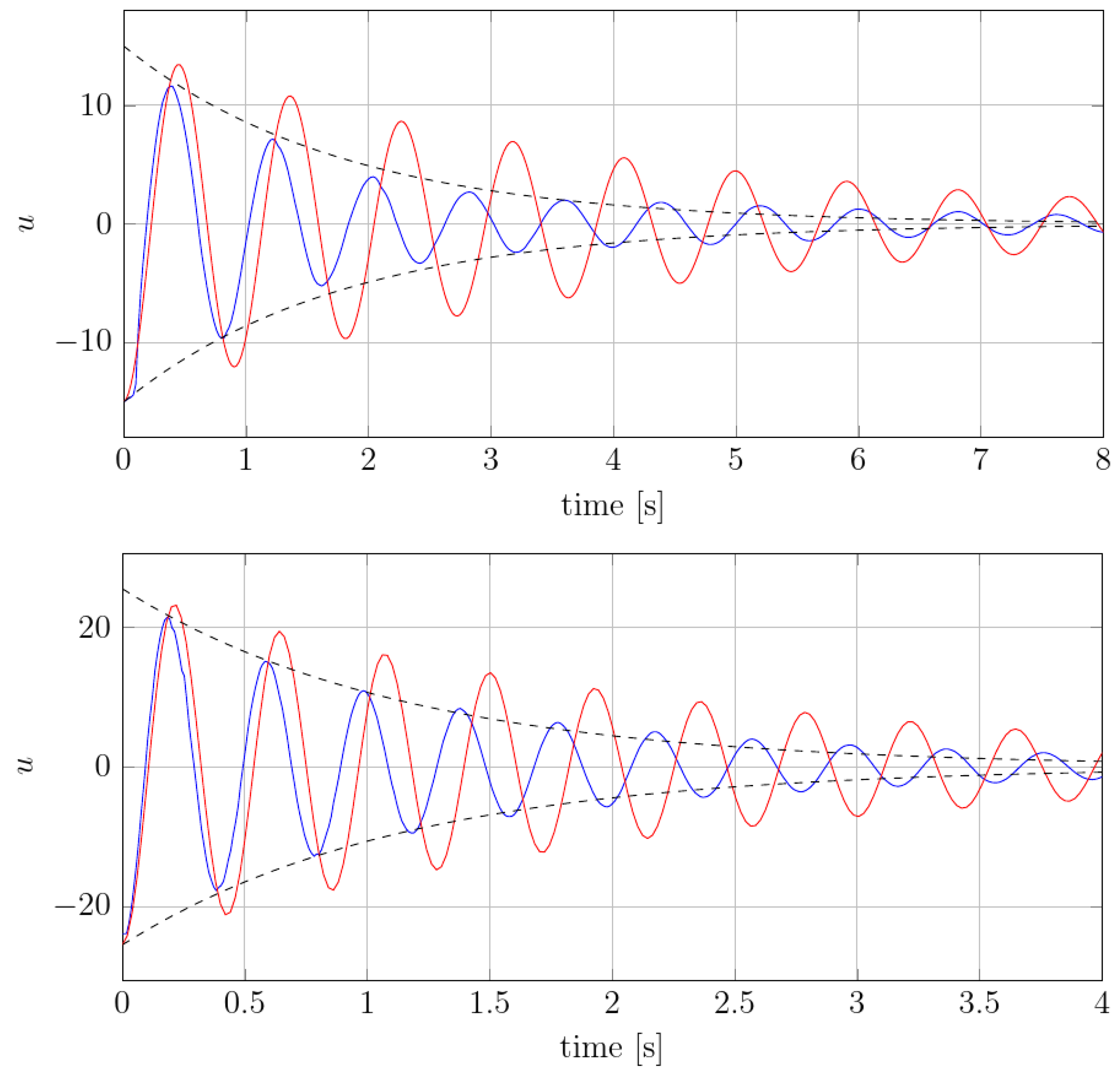
4.3. Hydroelastic Simulations

Transient hydroelastic simulations were performed with the FineMarine CFD solver, based on the numerical calculations described in Section 2.4. The Navier–Stokes equations were solved with the arbitrary Lagrangian–Eulerian (ALE) formulation, so that the RBF interpolation algorithm can be used to deform the CFD mesh according to the deformation of the structure, as explained in Section 3. Central-difference space discretisation was employed, and a four-stage explicit Runge–Kutta scheme was applied for the temporal discretisation. Time stepping was controlled such that one vibration period was discretised in at least 120 steps, while ensuring CFL criteria and minimal continuity residuals. After testing multiple meshes, a fluid mesh was built using 1.7 million of hexahedral cells around the barge, with the domain big enough to properly damp radiated waves and to capture all flow characteristics around the vibrating barge. Gaps between the pontoons were meshed with 40 layers of cells, and the no-slip boundary condition was imposed along with the Menter’s SST turbulence model. The structural modal damping ratio was set to 0.5% to include the damping caused by the hysteresis within the steel beams. The computational domain and the mesh refinement procedure were performed in similar way for the gapless monohull’s structural simulation.
Free vibrations in numerical simulations were initialised by releasing the structure deformed in the form of the specific mode shape depicted in Figure 3. The first two modes of vertical vibrations were simulated separately without mixing. Each hydroelastic simulation included exclusively one chosen mode of vibration. When the simulation was started, the barge vibrated with the wet natural frequency, which was lower than the input dry natural frequency due to the effects of water flow. Additional verification of the coupled solver was also done in terms of comparing the wet frequencies and added mass values obtained with the CFD to the values obtained with the surface panel method that uses distribution of singularities, i.e., sources of constant strength located on panels of the wetted surface [1]. The panel-method solution was obtained through the NASTRAN MFLUID solver on massless and infinitely stiff interface, which is presented in Section 4.2. These results are in agreement with the CFD results. The wet natural frequencies obtained from the experiment, CFD and FEM analysis is given in Table 3.
The experimental values were bounded by the numerical ones. The natural frequencies of the segmented barge are somewhat higher than those of the monohull. For the numerical evaluations, the relative difference of the second natural frequency rose higher from the first natural frequency than the difference from experimental frequencies. Therefore, it may seem the CFD and FEM monohull simulations get close to experimental results. Nevertheless, the CFD segmented simulation yielded a consistent relative difference compared to the experiments. It should be noted that in the case of the segmented barge, the restoring stiffness was lower due to gaps between barge segments. In addition, the added mass of the segmented barge was lower than that of monohull due to the pressure interaction between the segmented walls.
The modal acceleration, velocity and amplitude of a mode under consideration were tracked over time. Small gaps between the pontoons limited maximum initial deflection, to avoid intersection between pontoons. The first vertical vibration mode was initialised using the deflection that the tip of the barge was raised by about 10 cm, similarly to the experimental free-decay tests. Figure 4 shows that the modal acceleration slowly decays. The expected decay is drawn with a dashed line, which is based on extracted the damping ratio from the experimental analysis (given in Table 1). By applying the logarithmic decrement method from Section 2.3 onto the data of the simulated modal accelerations, it can be seen that the damping ratio, ζ , for the first mode of vibration, fluctuated from 5.5% to 8.2% of the critical damping; i.e., the damping ratio varied in time. The values were somewhat larger in the first vibration periods, and the vibrations dampened more slowly later in time, i.e., for lower vibration amplitudes. The expected decay was based on averaged value of the damping ratio; therefore, the numerically obtained values agree on average with the experiment.
The simulation of the second vertical vibration mode was initialised similarly to the first simulation, and the deflection had to be smaller due more complex mode shape and gaps between pontoons. Figure 4 shows decaying modal acceleration for the second vibration mode. By using the logarithmic decrement method, it can be seen that the damping ratio for the second mode of vibration fluctuated from 5.2% to 6.6% of the critical damping, which is in agreement with the experiment.
Contour plots of the free surface elevation during the simulation are shown in Figure 5 and Figure 6, for two modes of vibration, respectively. Wave elevation between the pontoon gaps is also visible from the profile view of the barge; see Figure 7 and Figure 8.

4.4. Discussion

By analysing Figure 5 and Figure 6, it may be seen that relatively far from the structure, wave elevation values formed similar contours for both the segmented and monohull simulations. It may be seen that for both vibrating modes, the shape and elevation of generated waves were similar far from the structure. The radiated waves formed bumps and hollows at similar locations relatively far from the structure, with the amplitude of approximately one centimetre for both modes. For the first mode of vibration, Figure 5 shows that a wave formed at the fore and aft shoulders as barge ends rising upwards (see Figure 9), and the generated wave from the midsection of the barge propagated in the transverse direction. For the second mode of vibration, the radiated waves in Figure 6 are even more similar, and wave hollows and bumps follow the motion of the mode shape shown in Figure 8. On the contrary, local wave generation is very complex in the vicinity of the vibrating segmented barge. The gaps generated trapped waves with amplitudes five times higher than those radiated from the structure. During a period of the vertical vibration, two effects are responsible for producing these localised waves that dissipate away from the structure. This localised ’pumping’ effect is also visible in Figure 7 and Figure 8. The first effect responsible for this phenomenon is the that the gaps change size and inclination during vibration. For example, a segment that is going upwards is gradually closing the gap at the keel, which creates gradient of the pressure in order to keep the incompressibility constraint (14) valid, which is pushing the fluid upwards. Similarly, the opposite holds when the structure is vibrating downwards, although the consequent negative elevation of the free surface is lower due to the smaller pressure gradient (at the free surface, the pressure value equals the ambient pressure). Figure 9 shows how the large pressure gradient creates large elevation of the free surface between gaps, and corresponding streamlines that verify the ’pumping’ effect. The second effect responsible for the phenomenon is the tangential (wall–velocity) boundary condition imposed on moving walls, which pulls or pushes the water using friction. Other than those two effects, another typical hydrodynamic effect affects the hydrodynamic damping (e.g., vortex creation around corners, as seen in Figure 9). Since the hydrodynamic damping may be defined as the energy loss during a vibration period due to hydrodynamic effects, it can be concluded that the described high-pressure gradients and additional friction are responsible for additional hydrodynamic damping during vibration of a segmented barge, compared to the monohull barge.

5. Conclusions

Model tests of segmented barges with very-low-in-rigidity steel backbones are usually performed for validation of a numerical procedure for hydroelastic behaviour of very large ships. However, in numerical analysis, the segmented barge is usually considered as a monohull. For this reason, numerical analyses for a segmented barge and a monohull barge were performed by coupling fluid and structural solvers using the mode analysis.
An efficient weak coupling method was described, which transfers flow-solver results onto the structure described by its mode shapes, each time step. The proposed coupling method for the unsteady deformation of the structure, by using a time integration of the mode shape, is stable and significantly faster than resolving the whole structure each time step. The results of damping and added mass effects were validated, rendering the method feasible for simulating vibrations of complex ships and floating structures.
Secondly, the results of the hydroelastic behaviour of the segmented barge, compared to its monohull counterpart, have answered the questions on why model tests of segmented floating structures are characterised by large hydrodynamic damping. The ’pumping’ effect, and the consequent generation of energy during a vibration period, is caused by the changing of gaps’ shapes. The shrinking and expansion of gaps generates large pressure gradients and produces localised elevation of the free surface. In addition, more vortices form and wall-shear grows, which also contributes to large hydrodynamic damping of segmented floating structures compared to the monohulls. In comparison to segmented floating structures (e.g., wave-energy converters), the stiffness of the ship is much higher and ship deformations are much lower so that it is possible to make the connection between the segments watertight using simple means (e.g., sellotape) without affecting the global stiffness.

References

Author Contributions

Conceptualization, J.B., N.D. and Š.M.; methodology, J.B., N.D. and Š.M.; software, J.B.; validation, N.D. and Š.M.; formal analysis, J.B. and N.D.; investigation, J.B., N.D. and Š.M.; resources, J.B.; data curation, J.B., N.D. and Š.M.; writing—original draft preparation, J.B., N.D. and Š.M.; writing—review and editing, J.B., N.D. and Š.M.; visualization, J.B.; supervision, N.D. All authors have read and agreed to the published version of the manuscript.

Funding

This study has been fully supported by the Croatian Science Foundation under project IP-2020-02-8568.

Institutional Review Board Statement

Not applicable.

Informed Consent Statement

Not applicable.

Data Availability Statement

Not applicable.

Acknowledgments

This study has been fully supported by the Croatian Science Foundation under project IP-2020-02-8568.

Conflicts of Interest

The authors declare no conflict of interest.

References

  1. Bašić, J.; Parunov, J. Analytical and Numerical Computation of Added Mass in Ship Vibration Analysis. Brodogradnja 2013, 64, 1–11. [Google Scholar]
  2. Abd Samad, F.I.; Mohd Yusop, M.Y.; Shaharuddin, N.M.R.; Ismail, N.; Yaakob, O.B. Slamming Impact Accelerations Analysis On Small High Speed Passenger Crafts. Brodogradnja 2021, 72, 79–94. [Google Scholar] [CrossRef]
  3. Kleivane, S.K.; Leira, B.J.; Steen, S. Development of a reliability model for crack growth occurrence for a secondary hull component. Brodogradnja 2023, 74, 99–115. [Google Scholar] [CrossRef]
  4. Kim, S.W.; Lee, S.J. Development Of A New Fatigue Damage Model For Quarter-Modal Spectra In Frequency Domain. Brodogradnja 2020, 71, 39–57. [Google Scholar] [CrossRef]
  5. Wenxi, L.; Huiren, G.; Qidou, Z.; Jingjun, L. Study On Structural-Acoustic Characteristics Of Cylindrical Shell Based On Wavenumber Spectrum Analysis Method. Brodogradnja 2021, 72, 57–71. [Google Scholar] [CrossRef]
  6. Jensen, J.J. Load and Global Response of Ships; Elsevier Ocean Engineering Series; Elsevier Science: Amsterdam, The Netherlands, 2001; pp. 268–271. [Google Scholar]
  7. Storhaug, G. Experimental Investigation of Wave Induced Vibrations and Their Effect on the Fatigue Loading of Ships. Ph.D Thesis, Norwegian University of Science and Technology, Trondheim, Norway, 2007. [Google Scholar]
  8. Storhaug, G. The measured contribution of whipping and springing on the fatigue and extreme loading of container vessels. Int. J. Nav. Archit. Ocean Eng. 2014, 6, 1096–1110. [Google Scholar] [CrossRef] [Green Version]
  9. Norwood, M.N.; Dow, R.S. Dynamic analysis of ship structures. Ships Offshore Struct. 2013, 8, 270–288. [Google Scholar] [CrossRef]
  10. Blake, W.K.; Chen, Y.K.; Walter, D.; Briggs, R. Design and Sea Trial Evaluation of the Containership MV Pfeiffer for Low Vibration. SNAME Trans. 1994, 102, 107–136. [Google Scholar]
  11. Colomés, O.; Verdugo, F.; Akkerman, I. A monolithic finite element formulation for the hydroelastic analysis of very large floating structures. Int. J. Numer. Methods Eng. 2023, 124, 714–751. [Google Scholar] [CrossRef]
  12. Chourdakis, G.; Davis, K.; Rodenberg, B.; Schulte, M.; Simonis, F.; Uekermann, B.; Abrams, G.; Bungartz, H.J.; Cheung Yau, L.; Desai, I.; et al. preCICE v2: A sustainable and user-friendly coupling library. Open Res. Eur. 2022, 2, 51. [Google Scholar] [CrossRef]
  13. Chen, Y.; Zhang, Y.; Tian, X.; Guo, X.; Li, X.; Zhang, X. A numerical framework for hydroelastic analysis of a flexible floating structure under unsteady external excitations: Motion and internal force/moment. Ocean Eng. 2022, 253, 111288. [Google Scholar] [CrossRef]
  14. Huang, H.; Chen, X.-j.; Liu, J.-y.; Ji, S. A method to predict hydroelastic responses of VLFS under waves and moving loads. Ocean Eng. 2022, 247, 110399. [Google Scholar] [CrossRef]
  15. Kashiwagi, M.; Kuga, S.; Chimoto, S. Time- and frequency-domain calculation methods for ship hydroelasticity with forward speed. In Proceedings of the 7th International Conference on Hydroelasticity in Marine Technology, Split, Croatia, 16–19 September 2015; pp. 477–492. [Google Scholar]
  16. Seng, S.; Jensen, J.J.; Malenica, S. Global hydroelastic model for springing and whipping based on a free-surface CFD code (OpenFOAM). Int. J. Nav. Archit. Ocean Eng. 2014, 6, 1024–1040. [Google Scholar] [CrossRef] [Green Version]
  17. Kumar Pal, S.; Iijima, K. Investigation of Springing Responses to High Harmonics of Wave Loads by Direct Coupling Between CFD and FEM. Volume 7: CFD and FSI. In Proceedings of the ASME 2022 41st International Conference on Ocean, Offshore and Arctic Engineering, Hamburg, Germany, 5–10 June 2022. [Google Scholar] [CrossRef]
  18. Kara, F. Time domain prediction of hydroelasticity of floating bodies. Appl. Ocean Res. 2015, 51, 1–13. [Google Scholar] [CrossRef]
  19. Debrabandere, F.; Tartinville, B.; Hirsch, C.; Coussement, G. Fluid-Structure Interaction Using a Modal Approach. J. Turbomach. 2012, 134, 51043. [Google Scholar] [CrossRef]
  20. Malenica, Š.; Molin, B.; Remy, F.; Senjanović, I. Hydroelastic response of a barge to impulsive and non-impulsive wave loads. In Proceedings of the 3rd International Conference on Hydroelasticity in Marine Technology, Oxford, UK, 15–17 September 2003; p. 9. [Google Scholar]
  21. Piro, D.J.; Maki, K.J. Whipping Response of a Box Barge in Oblique Seas. In Proceedings of the 28th International Workshop on Water Waves and Floating Bodies, Marseille, France, 7–10 April 2013; pp. 173–176. [Google Scholar]
  22. Bašić, J.; Degiuli, N.; Dejhalla, R. Total resistance prediction of an intact and damaged tanker with flooded tanks in calm water. Ocean Eng. 2017, 130, 83–91. [Google Scholar] [CrossRef]
  23. Andrun, M.; Blagojević, B.; Bašić, J. The influence of numerical parameters in the finite-volume method on the Wigley hull resistance. Proc. Inst. Mech. Eng. Part M J. Eng. Marit. Environ. 2019, 233, 1123–1132. [Google Scholar] [CrossRef]
  24. Andrun, M.; Blagojević, B.; Bašić, J.; Klarin, B. Impact of CFD simulation parameters in prediction of ventilated flow on a surface-piercing hydrofoil. Ship Technol. Res. 2021, 68, 1–13. [Google Scholar] [CrossRef]
  25. De Boer, A.; van der Schoot, M.; Bijl, H. Mesh deformation based on radial basis function interpolation. Comput. Struct. 2007, 85, 784–795. [Google Scholar] [CrossRef]
Figure 1. The geometry of the flexible segmented barge (dimensions are in mm).
Jmse 11 00581 g001
Figure 2. Finite element model of the barge (red— beam elements, blue—plate elements, black—mass elements, white—rigid connections).
Jmse 11 00581 g002
Figure 3. First three shape modes of vertical vibration of a flexible barge.
Jmse 11 00581 g003
Figure 4. Modal acceleration of first (top) and second (bottom) vibration modes for the segmented model (blue) and monohull (red), compared to the decay based on experimental modal damping ratio (dashed line).
Jmse 11 00581 g004
Figure 5. Top view of free surface elevation contours for the first mode of vertical vibration (segmented hull—top image, monohull—bottom image).
Jmse 11 00581 g005
Figure 6. Top view of free surface elevation contours for the second mode of vertical vibration (segmented hull—top image, monohull—bottom image).
Jmse 11 00581 g006
Figure 7. Profile view of free-surface elevation along the barge’s length for the first mode of vertical vibration.
Jmse 11 00581 g007
Figure 8. Profile view of free surface elevation along the barge’s length for the second mode of vertical vibration.
Jmse 11 00581 g008
Figure 9. Section cut at the centreline, showing streamlines and the dynamic pressure field for the first mode of vertical vibration of the segmented barge.
Jmse 11 00581 g009
Table 1. Wet natural frequencies and damping ratios for the first two vibration modes, obtained using the modal analysis and experimental data.
ModeNatural Frequency ω i Average Damping Ratio ζ i
11.24 Hz7.3%
22.40 Hz6.2%
Table 2. Dry natural frequencies obtained analytically and numerically, in Hz; relative differences compared with the analytical solution.
ModeTimoshenkoFEM, Mass Above DeckRelative DifferenceFEM, Figure 2Relative Difference
11.367 Hz1.389 Hz+1.6%1.295 Hz−5.3%
23.769 Hz3.823 Hz+1.4%3.346 Hz−11.2%
37.389 Hz7.487 Hz+1.3%5.900 Hz−20.1%
Table 3. Wet natural frequencies for the first two vibration modes, in Hz, obtained with different methods and models.
ModeExperimentCFD, SegmentedRelative DifferenceCFD, MonohullRelative DifferenceFEM, MonohullRelative Difference
11.24 Hz1.26 Hz+1.6%1.12 Hz−9.7%1.02 Hz−17.7%
22.40 Hz2.54 Hz+5.8%2.33 Hz−2.9%2.48 Hz+3.3%
Disclaimer/Publisher’s Note: The statements, opinions and data contained in all publications are solely those of the individual author(s) and contributor(s) and not of MDPI and/or the editor(s). MDPI and/or the editor(s) disclaim responsibility for any injury to people or property resulting from any ideas, methods, instructions or products referred to in the content.

