

Visual Odometry-Based Robust Control for an Unmanned Surface Vehicle under Waves and Currents in a Urban Waterway

Abstract
:1. Introduction
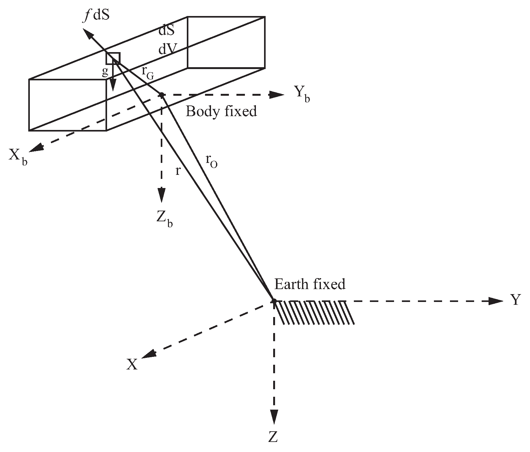
2. System Modeling
2.1. USV Model
2.2. Environmental Disturbances
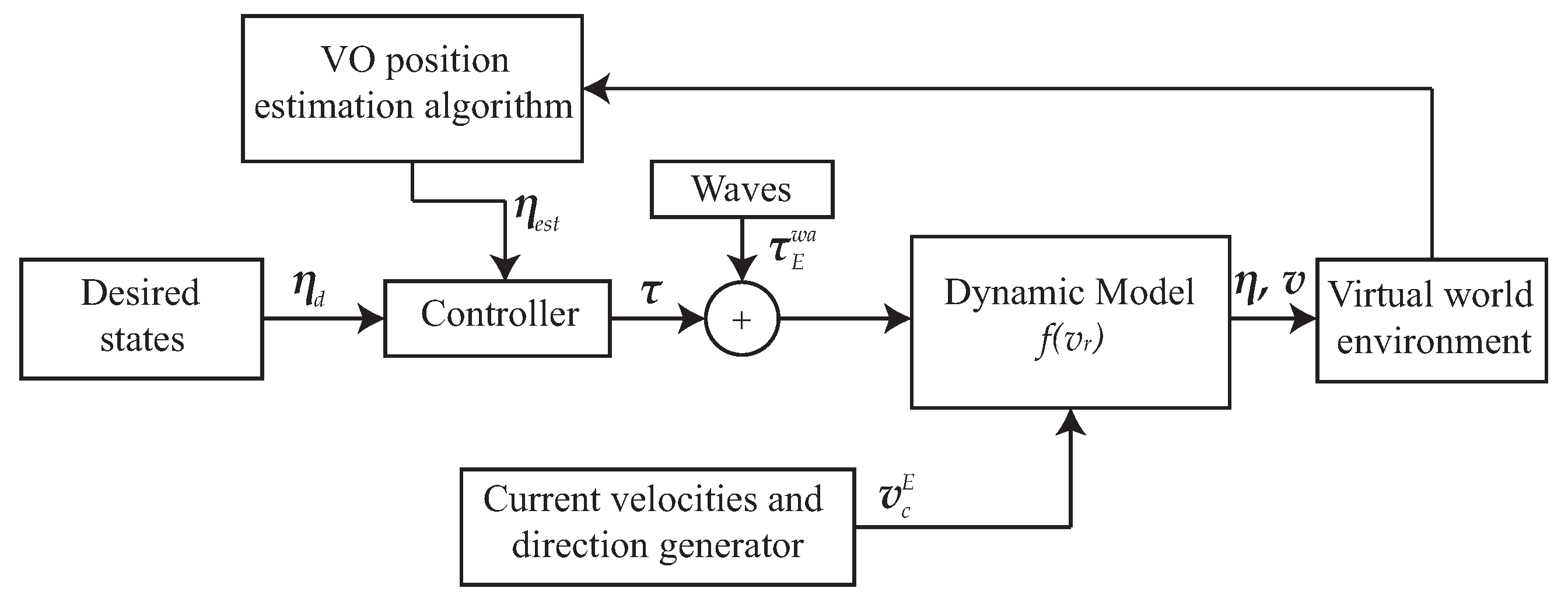
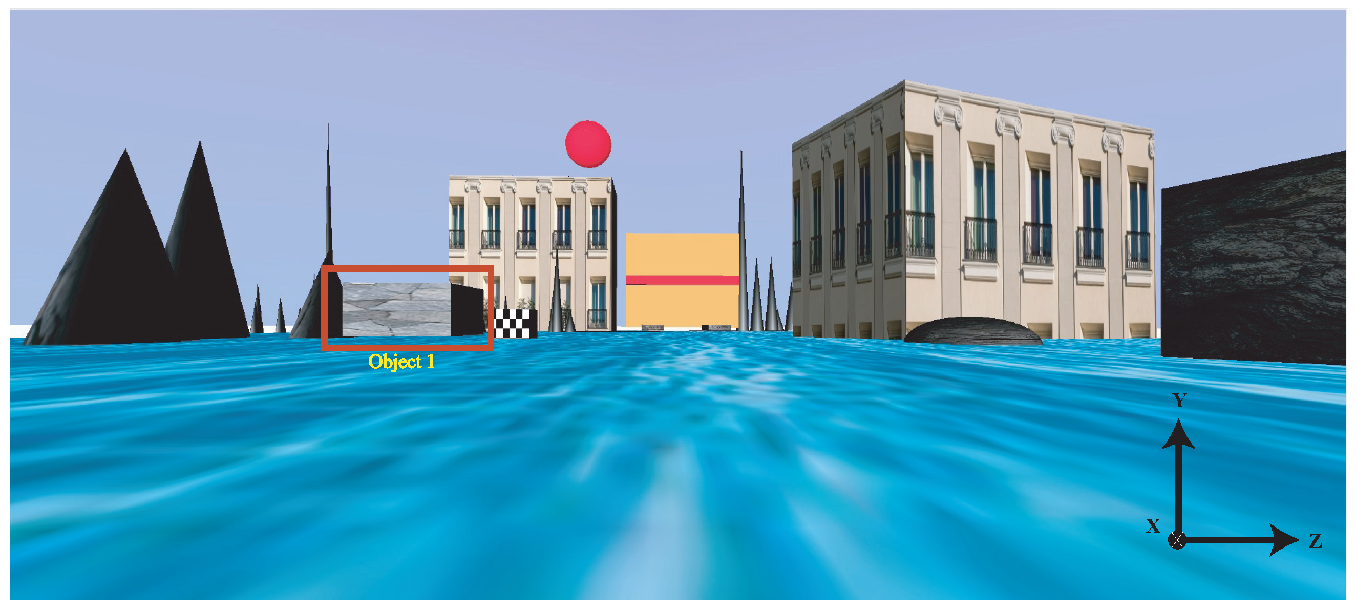
3. Robust Control Based on Visual Position Estimation
3.1. VO Mathematical Background
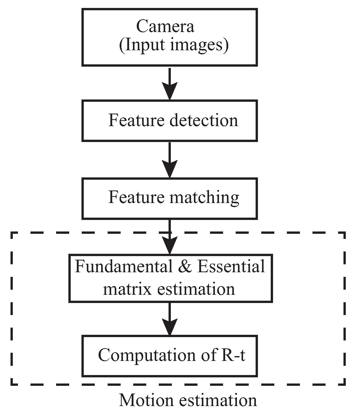
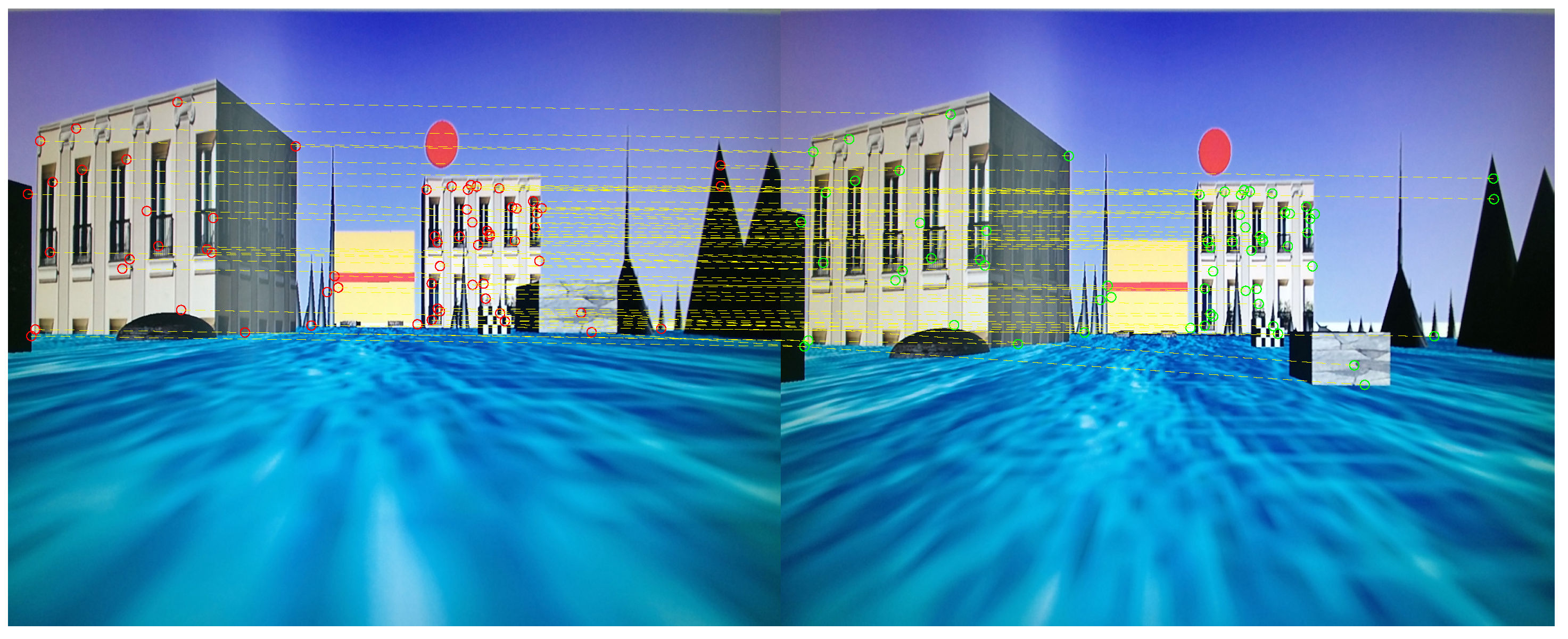
3.2. Monocular Visual Odometry
- 1.
- Capture a new input image .
- 2.
- Detection and matching of features between the new () and old () image.
- 3.
- Compute fundamental matrix F with RANSAC for outlier rejection.
- 4.
- Compute essential matrix from fundamental matrix.
- 5.
- Extract R and t from essential matrix using SVD.
- 6.
- Use cheirality constraint to obtain the true configuration.
- 7.
- Perform scale adjustment.
- 8.
- Concatenate transformation.
- 9.
- Repeat from step 1.
3.3. Control Design
Stability Analysis
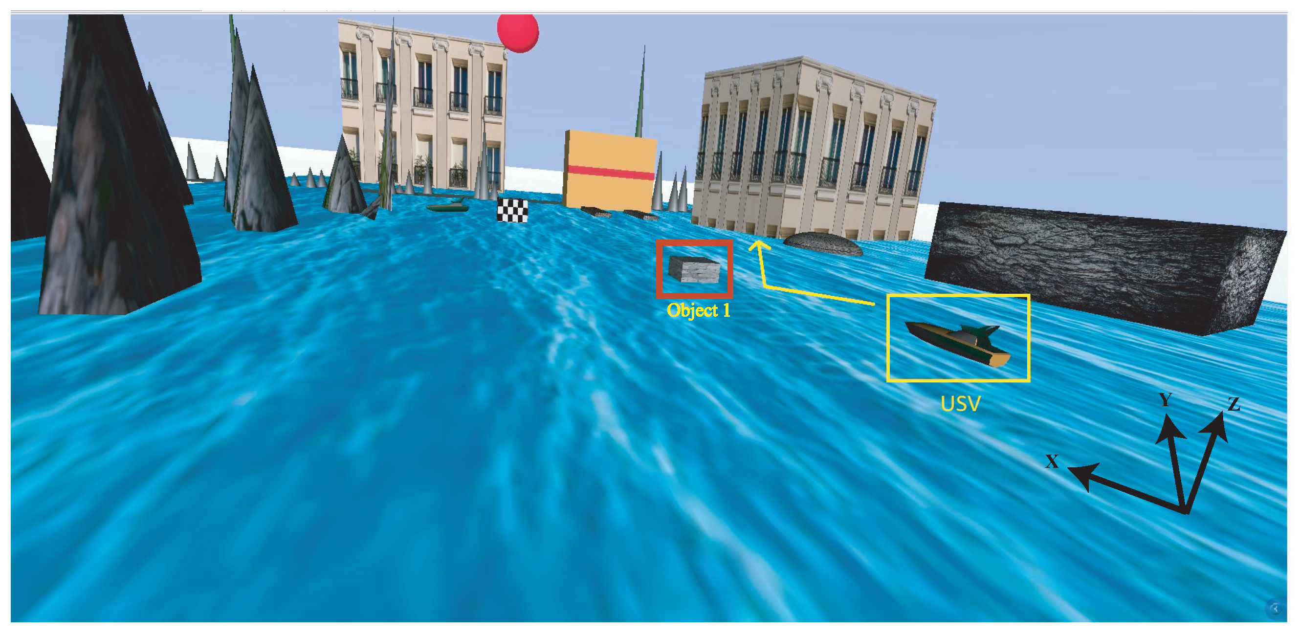
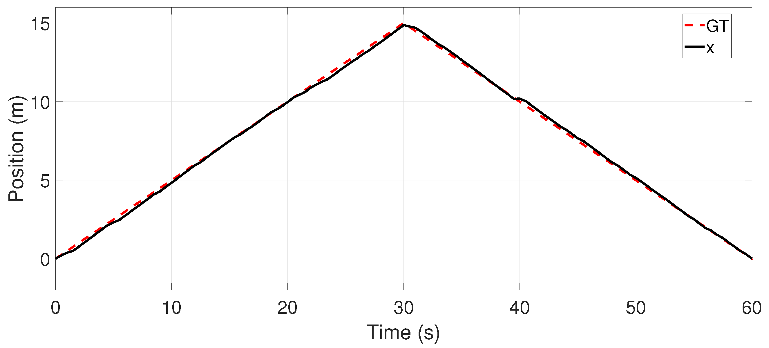
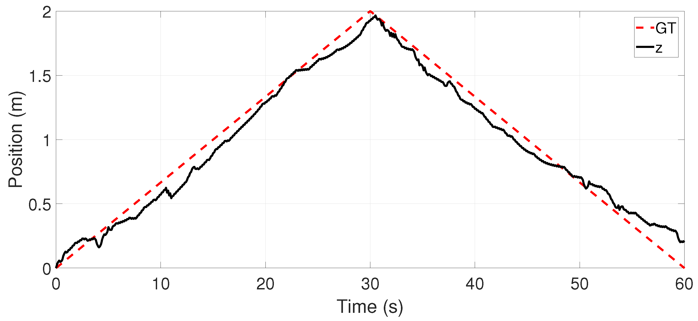
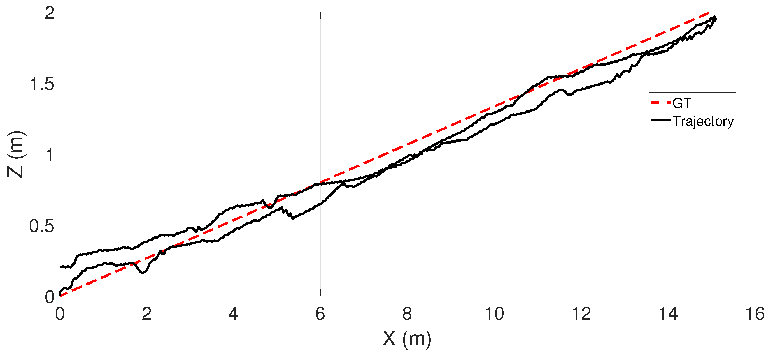
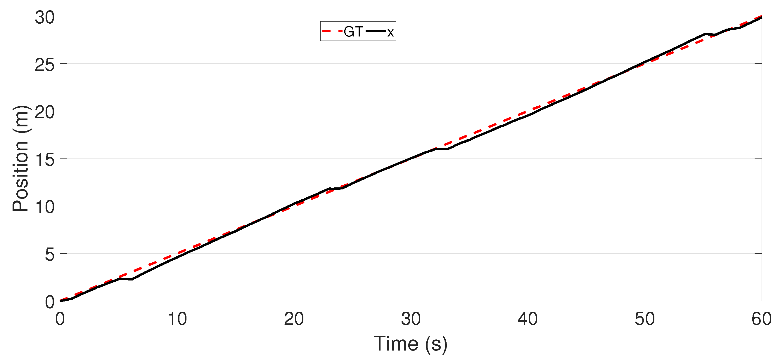
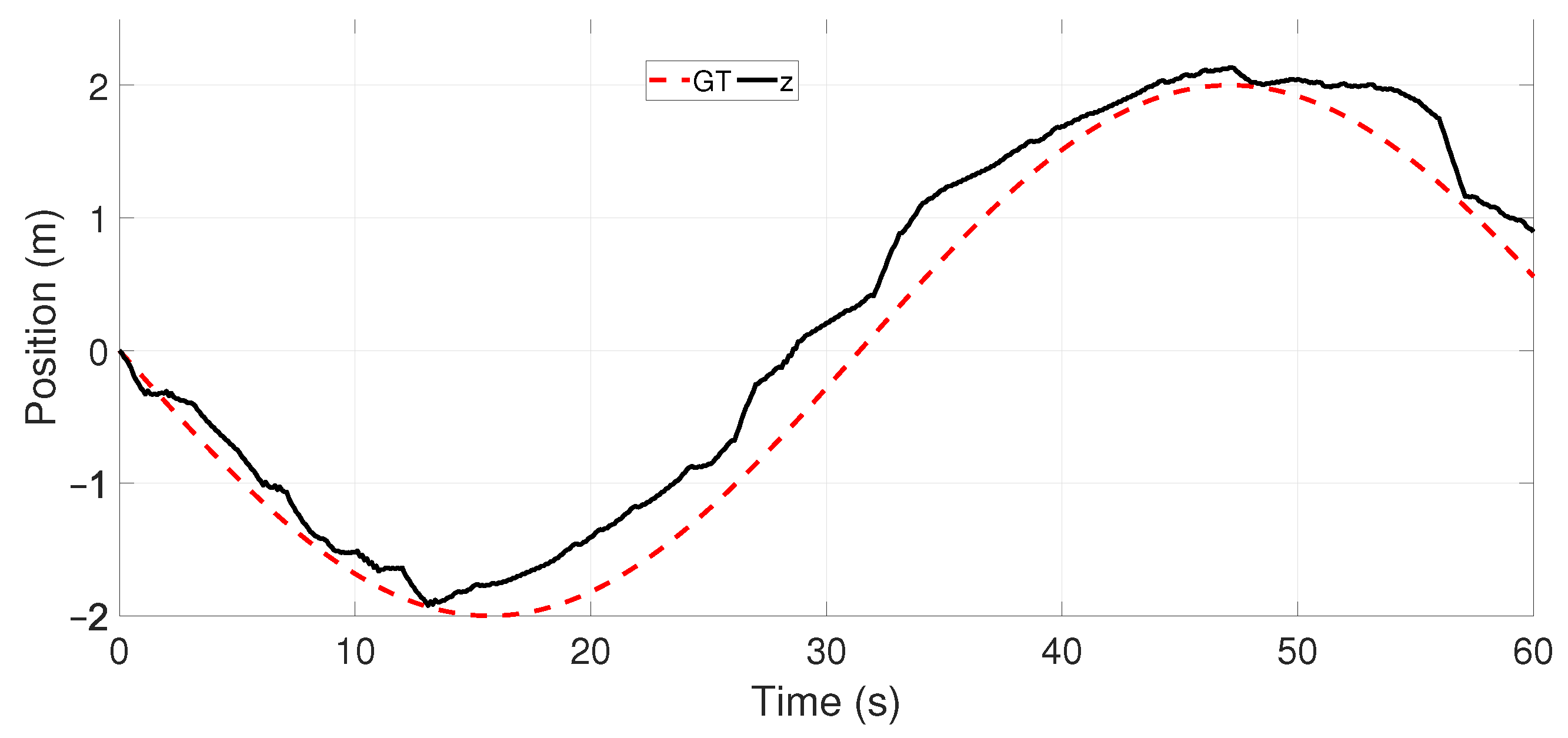
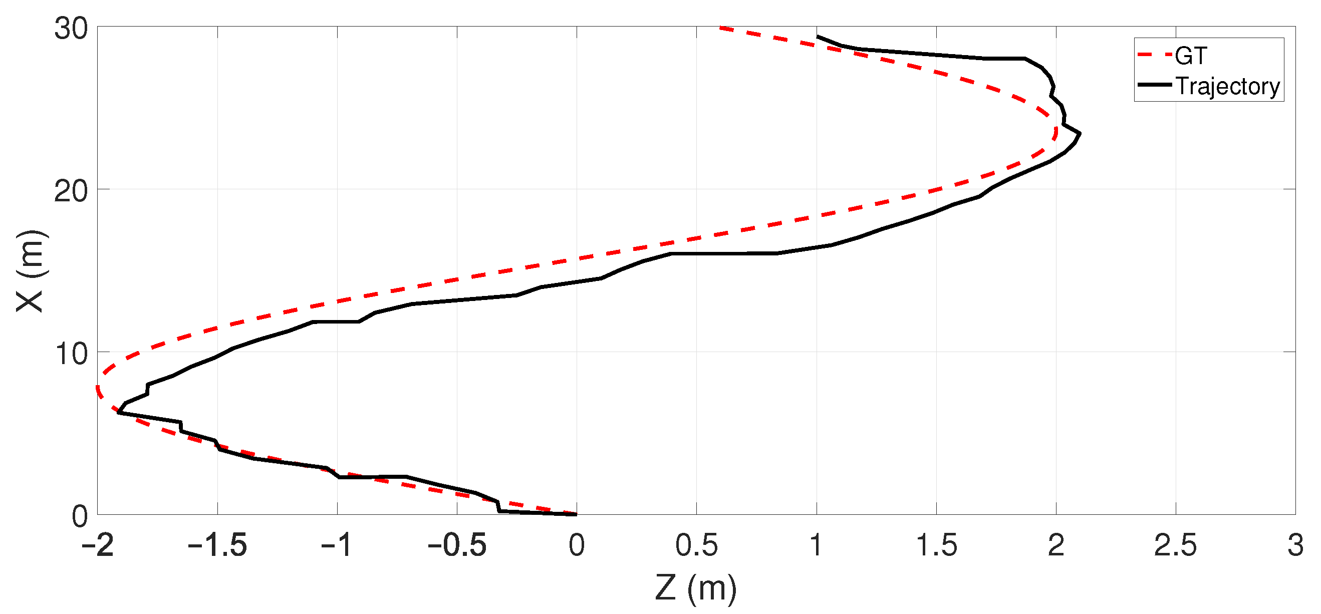
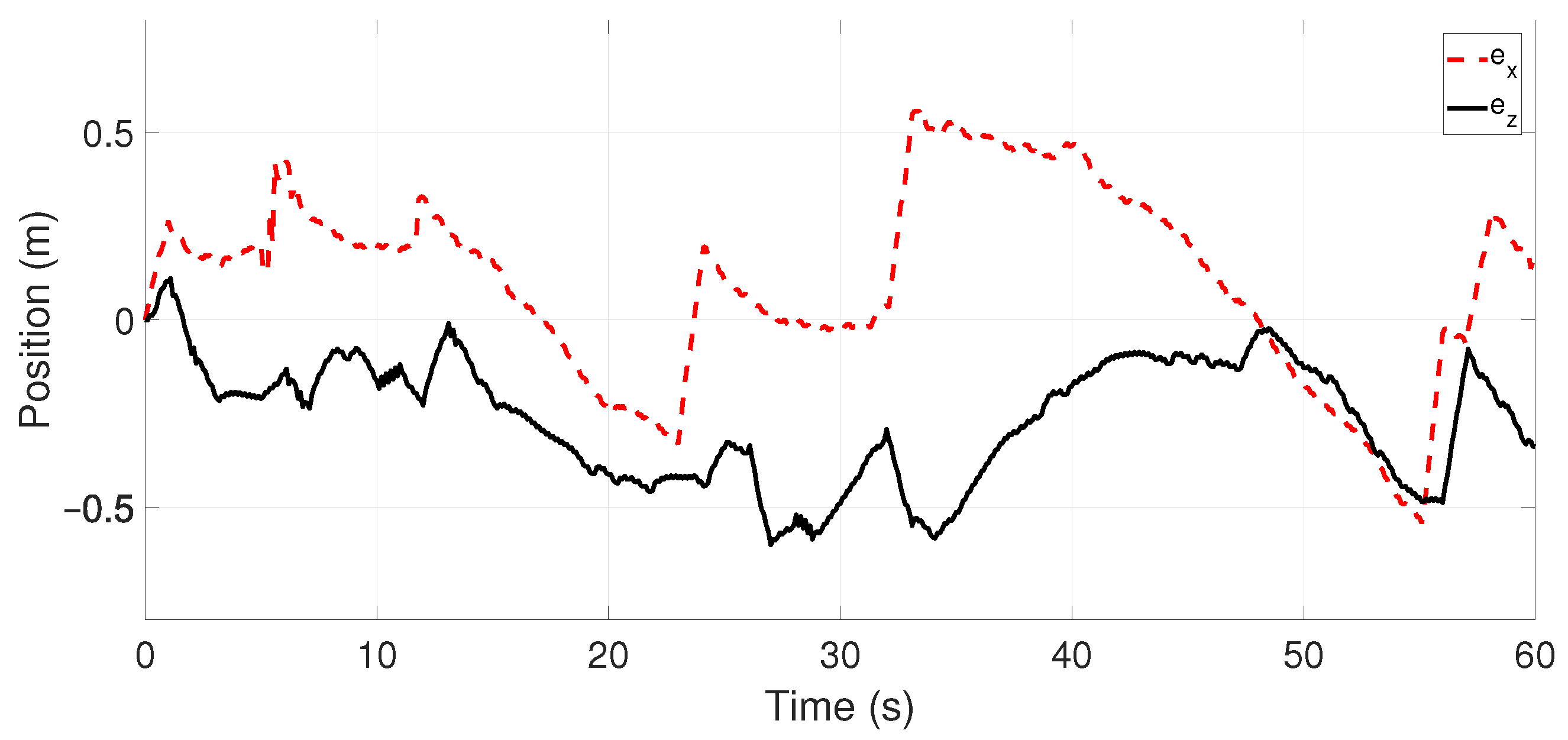
4. Results
5. Conclusions
Author Contributions
Funding
Institutional Review Board Statement
Informed Consent Statement
Data Availability Statement
Conflicts of Interest
References
- Yan, R.J.; Pang, S.; Sun, H.B.; Pang, Y.J. Development and missions of unmanned surface vehicle. J. Mar. Sci. Appl. 2010, 9, 451–457. [Google Scholar] [CrossRef]
- Jorge, V.A.; Granada, R.; Maidana, R.G.; Jurak, D.A.; Heck, G.; Negreiros, A.P.; Dos Santos, D.H.; Gonçalves, L.M.; Amory, A.M. A survey on unmanned surface vehicles for disaster robotics: Main challenges and directions. Sensors 2019, 19, 702. [Google Scholar] [CrossRef] [PubMed] [Green Version]
- Naeem, W.; Sutton, R.; Chudley, J. Modelling and control of an unmanned surface vehicle for environmental monitoring. In Proceedings of the UKACC International Control Conference, Glasgow, UK, 30 August–1 September 2006; pp. 1–6. [Google Scholar]
- Madeo, D.; Pozzebon, A.; Mocenni, C.; Bertoni, D. A low-cost unmanned surface vehicle for pervasive water quality monitoring. IEEE Trans. Instrum. Meas. 2020, 69, 1433–1444. [Google Scholar] [CrossRef]
- Fossen, T.I. Nonlinear Modelling and Control of Underwater Vehicles. Ph.D. Thesis, Universitetet i Trondheim, Trondheim, Norway, 1991. [Google Scholar]
- Fossen, T.I. Marine Control Systems Guidance, Navigation, and Control of Ships, Rigs and Underwater Vehicles; Marine Cybernetics: Trondheim, Norway, 2002. [Google Scholar]
- Li, C.; Jiang, J.; Duan, F.; Liu, W.; Wang, X.; Bu, L.; Sun, Z.; Yang, G. Modeling and experimental testing of an unmanned surface vehicle with rudderless double thrusters. Sensors 2019, 19, 2051. [Google Scholar] [CrossRef] [PubMed] [Green Version]
- Zhang, R.; Liu, Y.; Anderlini, E. Robust trajectory tracking control for unmanned surface vessels under motion constraints and environmental disturbances. Proc. Inst. Mech. Eng. Part M J. Eng. Marit. Environ. 2022, 236, 394–411. [Google Scholar] [CrossRef]
- Shojaei, K. Neural adaptive robust control of underactuated marine surface vehicles with input saturation. Appl. Ocean Res. 2015, 53, 267–278. [Google Scholar] [CrossRef]
- Lv, C.; Yu, H.; Zhao, N.; Chi, J.; Liu, H.; Li, L. Robust state-error port-controlled Hamiltonian trajectory tracking control for unmanned surface vehicle with disturbance uncertainties. Asian J. Control 2022, 24, 320–332. [Google Scholar] [CrossRef]
- Qiu, B.; Wang, G.; Fan, Y.; Mu, D.; Sun, X. Adaptive sliding mode trajectory tracking control for unmanned surface vehicle with modeling uncertainties and input saturation. Appl. Sci. 2019, 9, 1240. [Google Scholar] [CrossRef] [Green Version]
- Nistér, D.; Naroditsky, O.; Bergen, J. Visual odometry. In Proceedings of the 2004 IEEE Computer Society Conference on Computer Vision and Pattern Recognition (CVPR 2004), Washington, DC, USA, 27 June–2 July 2004; Volume 1, p. I. [Google Scholar]
- Scaramuzza, D.; Fraundorfer, F. Visual odometry [tutorial]. IEEE Robot. Autom. Mag. 2011, 18, 80–92. [Google Scholar] [CrossRef]
- Hartley, R.; Zisserman, A. Multiple View Geometry in Computer Vision; Cambridge university Press: Cambridge, UK, 2003. [Google Scholar]
- Mostafa, M.Z.; Khater, H.A.; Rizk, M.R.; Bahasan, A.M. A novel GPS/RAVO/MEMS-INS smartphone-sensor-integrated method to enhance USV navigation systems during GPS outages. Meas. Sci. Technol. 2019, 30, 095103. [Google Scholar] [CrossRef]
- Balamurugan, G.; Valarmathi, J.; Naidu, V. Survey on UAV navigation in GPS denied environments. In Proceedings of the 2016 International conference on signal processing, communication, power and embedded system (SCOPES), Paralakhemundi, India, 3–5 October 2016; pp. 198–204. [Google Scholar]
- Maimone, M.; Cheng, Y.; Matthies, L. Two years of visual odometry on the mars exploration rovers. J. Field Robot. 2007, 24, 169–186. [Google Scholar] [CrossRef] [Green Version]
- Dunbabin, M.; Usher, K.; Corke, P. Visual motion estimation for an autonomous underwater reef monitoring robot. In Field and Service Robotics; Springer: Berlin/Heidelberg, Germany, 2006; pp. 31–42. [Google Scholar]
- Raimondi, F.M.; Trapanese, M.; Franzitta, V.; Viola, A.; Colucci, A. A innovative semi-immergible USV (SI-USV) drone for marine and lakes operations with instrumental telemetry and acoustic data acquisition capability. In Proceedings of the OCEANS 2015—Genova, Genova, Italy, 18–21 May 2015; pp. 1–10. [Google Scholar] [CrossRef]
- Chen, L.; Huang, Y.; Zheng, H.; Hopman, H.; Negenborn, R. Cooperative multi-vessel systems in urban waterway networks. IEEE Trans. Intell. Transp. Syst. 2019, 21, 3294–3307. [Google Scholar] [CrossRef] [Green Version]
- Balbuena, J.; Quiroz, D.; Song, R.; Bucknall, R.; Cuellar, F. Design and implementation of an USV for large bodies of fresh waters at the highlands of Peru. In Proceedings of the OCEANS 2017—Anchorage, Anchorage, AK, USA, 18–21 September 2017; pp. 1–8. [Google Scholar]
- Wang, W.; Gheneti, B.; Mateos, L.A.; Duarte, F.; Ratti, C.; Rus, D. Roboat: An autonomous surface vehicle for urban waterways. In Proceedings of the 2019 IEEE/RSJ International Conference on Intelligent Robots and Systems (IROS), Macau, China, 3–8 November 2019; pp. 6340–6347. [Google Scholar]
- Sinisterra, A.J.; Dhanak, M.R.; Von Ellenrieder, K. Stereovision-based target tracking system for USV operations. Ocean Eng. 2017, 133, 197–214. [Google Scholar] [CrossRef]
- Han, J.; Cho, Y.; Kim, J. Coastal SLAM with marine radar for USV operation in GPS-restricted situations. IEEE J. Ocean. Eng. 2019, 44, 300–309. [Google Scholar] [CrossRef]
- Uyar, E.; Alpkaya, A.T.; Mutlu, L. Dynamic modelling, investigation of manoeuvring capability and navigation control of a cargo ship by using matlab simulation. IFAC-PapersOnLine 2016, 49, 104–110. [Google Scholar] [CrossRef]
- Gonzalez-Garcia, A.; Castañeda, H. Guidance and control based on adaptive sliding mode strategy for a USV subject to uncertainties. IEEE J. Ocean. Eng. 2021, 46, 1144–1154. [Google Scholar] [CrossRef]
- Skjetne, R.; Fossen, T.I.; Kokotović, P.V. Adaptive maneuvering, with experiments, for a model ship in a marine control laboratory. Automatica 2005, 41, 289–298. [Google Scholar] [CrossRef]
- Coe, R.G.; Bacelli, G.; Wilson, D.G.; Abdelkhalik, O.; Korde, U.A.; Robinett III, R.D. A comparison of control strategies for wave energy converters. Int. J. Mar. Energy 2017, 20, 45–63. [Google Scholar] [CrossRef]
- Dunbabin, M.; Grinham, A.; Udy, J. An autonomous surface vehicle for water quality monitoring. In Proceedings of the Australasian Conference on Robotics and Automation (ACRA), Sydney, Australia, 2–4 December 2009; pp. 2–4. [Google Scholar]
- Do, K.D.; Pan, J. Control of Ships and Underwater Vehicles: Design for Underactuated and Nonlinear Marine Systems; Springer: London, UK, 2009; Volume 1. [Google Scholar]
- Fossen, T.I. How to incorporate wind, waves and ocean currents in the marine craft equations of motion. IFAC Proc. Vol. 2012, 45, 126–131. [Google Scholar] [CrossRef] [Green Version]
- Collado-Gonzalez, I.; Gonzalez-Garcia, A.; Sotelo, C.; Sotelo, D.; Castañeda, H. A Real-Time NMPC Guidance Law and Robust Control for an Autonomous Surface Vehicle. IFAC-PapersOnLine 2021, 54, 252–257. [Google Scholar] [CrossRef]
- Davies, E.R. Computer Vision: Principles, Algorithms, Applications, Learning; Academic Press: Cambridge, MA, USA, 2017. [Google Scholar]
- Nistér, D. Preemptive RANSAC for live structure and motion estimation. Mach. Vis. Appl. 2005, 16, 321–329. [Google Scholar] [CrossRef] [Green Version]
- Tsai, R.Y.; Huang, T.S. Uniqueness and estimation of three-dimensional motion parameters of rigid objects with curved surfaces. IEEE Trans. Pattern Anal. Mach. Intell. 1984, PAMI-6, 13–27. [Google Scholar] [CrossRef] [PubMed] [Green Version]
- Almeida, J.; Silvestre, C.; Pascoal, A. Path-following control of fully-actuated surface vessels in the presence of ocean currents. IFAC Proc. Vol. 2007, 40, 26–31. [Google Scholar] [CrossRef] [Green Version]
- Utkin, V.; Guldner, J.; Shi, J. Sliding Mode Control in Electro-Mechanical Systems; CRC Press: Boca Raton, FL, USA, 2017. [Google Scholar]
- Oyallon, E.; Rabin, J. An analysis of the SURF method. Image Process. On Line 2015, 5, 176–218. [Google Scholar] [CrossRef]


Disclaimer/Publisher’s Note: The statements, opinions and data contained in all publications are solely those of the individual author(s) and contributor(s) and not of MDPI and/or the editor(s). MDPI and/or the editor(s) disclaim responsibility for any injury to people or property resulting from any ideas, methods, instructions or products referred to in the content. |
© 2023 by the authors. Licensee MDPI, Basel, Switzerland. This article is an open access article distributed under the terms and conditions of the Creative Commons Attribution (CC BY) license (https://creativecommons.org/licenses/by/4.0/).
Share and Cite
Cortes-Vega, D.; Alazki, H.; Rullan-Lara, J.L. Visual Odometry-Based Robust Control for an Unmanned Surface Vehicle under Waves and Currents in a Urban Waterway. J. Mar. Sci. Eng. 2023, 11, 515. https://doi.org/10.3390/jmse11030515
Cortes-Vega D, Alazki H, Rullan-Lara JL. Visual Odometry-Based Robust Control for an Unmanned Surface Vehicle under Waves and Currents in a Urban Waterway. Journal of Marine Science and Engineering. 2023; 11(3):515. https://doi.org/10.3390/jmse11030515
Chicago/Turabian StyleCortes-Vega, David, Hussain Alazki, and Jose Luis Rullan-Lara. 2023. "Visual Odometry-Based Robust Control for an Unmanned Surface Vehicle under Waves and Currents in a Urban Waterway" Journal of Marine Science and Engineering 11, no. 3: 515. https://doi.org/10.3390/jmse11030515