Analysis and Experimental Research on Efficiency Characteristics of a Deep-Sea Hydraulic Power Source

Abstract

The deep-sea environment has the characteristics of high pressure and low temperature. In addition to the extremely high requirements on the structural reliability, the ultra-high ambient pressure also has a great impact on the working characteristics of the hydraulic source. In this paper, the efficiency characteristics of a deep-sea hydraulic source are studied in the full-ocean-depth pressure range. According to the power transfer process, the efficiency of the deep-sea motor, gear pump and hydraulic circuit is analyzed. In so doing, the oil friction loss of the motor rotor, the internal leakage of the gear pump, the viscous friction loss of the hydraulic system, etc., are calculated. Then, simulating the deep-sea high-pressure environment by the pressure cylinder, the output characteristics and corresponding input power of the prototype are measured. By analyzing the experimental data, the efficiency characteristic curve of the hydraulic source prototype, changing with the ambient pressure, is obtained. The experimental and calculation results show that, with the increase of ambient pressure, the system efficiency of the hydraulic source prototype increases first and then decreases.

1. Introduction

Most of the earth’s surface is covered by oceans, and human exploration of oceans is still very limited. Therefore, the submersibles of Unmanned Surface Vehicles, Underwater Glider, etc., and corresponding integrated components can be designed and developed [1,2,3,4]. Compared with the easily accessible shallow sea areas, the deep sea puts forward higher technical requirements for marine equipment, where the high pressure, extreme darkness, and radio attenuation prevent direct access [5,6].

As an important tool for exploring the deep sea, the technological development of submersibles is also a research hotspot. Mainly include Remote Operated Vehicle (ROV), Autonomous Underwater Vehicle (AUV), and Human Occupied Vehicle (HOV). With the continuous exploration of the deep sea, humans have been trying to challenge the deepest Challenger Deep. The successful diving of the “Trieste” HOV in 1960 marked the first successful attempt in human history. The “Kaikō” ROV and “Nereus” HROV completed 10,000-m unmanned diving in 1996 and 2009. In 2012, the most famous HOV “Deepsea Challenger” carried James Cameron to complete the second 10,000-m manned diving after 1960. China’s “Fendouzhe” HOV and ‘Haidou-1’ ARV also completed 10,000-m manned and unmanned deep diving in 2020 and 2021 [7]. However, the exploration of the full ocean depth was not always smooth. In 2003, the steel secondary cable of “Kaikō” was broken, and the ROV was missing in deep water. In 2014, the “Nereus” had a catastrophic implosion during a deep dive at the Kermadec Trench. The “Deepsea Challenger” aboard James Cameron leaked oil on the seabed, resulting in the shutdown of the propeller and being forced to float in advance. In the past two years, the US’s “DSV Limiting Factor” and China’s “Fendouzhe” full-ocean-depth manned submersibles have shown good reliability and completed many 10,000-m deep dives. It is undeniable that the full-ocean-depth pressure environment puts forward extremely high requirements for the design and manipulation of submersibles.

Deep-sea submersibles generally carry hydraulic power systems and hydraulic actuators [8,9]. Most of the hydraulic power sources are designed as a closed structure. The closed structure has high integration, which can make the system more compact and easy to connect with various actuators. The oil-based underwater hydraulic source is generally composed of oil tank, pressure compensator, underwater motor, sensors, and valve box. The size of the tank determines the sustainable operation time of the system. The oil tank also cools the mineral oil, reduces air and cleans contaminants [10]. The pressure compensator can balance the ambient pressure and the internal pressure, so as to avoid the system structure being directly oppressed by the external pressure and corroded by the seawater [11,12].

Cao [13] established the mathematical models of the hydraulic system and electrical system of a deep-sea hydraulic source by linear varying parameters (LVP) method. In the bounded closed set of variable parameters, the dynamic characteristics of pressure and flow are obtained. The rationality of the LVP method is verified by experiments. Zhou [14] theoretically analyzed the efficiency of deep-sea motors and hydraulic pumps. The CFD simulation of the internal gear pump was carried out, and the influence of hydraulic oil viscosity change on pump power loss was analyzed. Liu [15] theoretically analyzed the dynamic characteristics of electro-hydraulic servo valve in deep sea environment. The deformation of valve spool and sleeve under different pressures was simulated, and the dynamic characteristics of servo valve with different clearances size were obtained by Simulink. Wang [16] analyzed the pressure compensator of the deep-sea hydraulic system. The steady-state characteristics of the spring-piston pressure compensator are studied. The output state of the hydraulic source prototype with a pressure compensator was observed through the camera. Li [17] studied the power loss of deep-sea BLDC motors. The effects of ambient pressure on the oil friction loss and the magnetic properties of the silicon steel sheet are mainly studied. The temperature field of the underwater oil-immersed motor is calculated by the indirect coupling method.

Based on the characteristics of high pressure and low temperature in deep sea, the above articles analyze the possible effect on the components of hydraulic system. In this paper, the efficiency characteristics of the deep-sea hydraulic source are studied in the full-ocean-depth pressure range. According to the power transfer process, the efficiency of the deep-sea motor, gear pump and hydraulic circuit is analyzed. In which, the oil friction loss of the motor rotor, the internal leakage of the gear pump, the viscous friction loss of the hydraulic system, etc. are mainly calculated. The calculation results show that with the increase of ambient pressure, the efficiency of the deep-sea motor gradually decreases, while the efficiency of the hydraulic system increases first and then decreases. Simulating the deep-sea high-pressure environment by the pressure cylinder, the output characteristics and corresponding input power of the prototype are measured. By analyzing the experimental data, the efficiency characteristic curve of the hydraulic source prototype, changing with the environmental pressure, is obtained. The experimental results are consistent with the calculated results. With the increase of ambient pressure, the system efficiency of the hydraulic source prototype increases first and then decreases. In deep-sea environments, the frictional power loss due to viscous fluids is the main reason for the reduction in system efficiency.

2. System Principle

2.1. System Structure

Sealing and pressure-resistant performance are the key points in the structural design of deep-sea hydraulic sources. The ultra-high external pressure has high requirements for the strength of the closed shell, so it is necessary to set up a flexible structure with variable volume. The internal pressure is increased by compressing the oil volume, so that the internal and external pressures can be balanced. The deep-sea hydraulic source system is limited by volume, and the temperature of the working oil increases rapidly when it circulates in the oil tank. Therefore, it is necessary to install a radiator in the circuit to suppress the temperature rise.

The specific work indicators of the system are as follows:

(1)

Maximum working ambient pressure: 115 MPa.

(2)

Maximum resistant ambient pressure: 144 MPa.

(3)

Maximum output pressure: 21 MPa.

(4)

Maximum output flow > 10 L/min.

Figure 1 is the principle diagram of the system. The hydraulic source system is a closed cavity structure, and the hydraulic and electrical components are oil-immersed installation. The internal and external pressures of the oil tank are balanced by the pressure compensator, which reduces the load on the tank and improves overall structural safety. The motor and gear pump are also oil-immersed and placed separately in the motor cylinder.

The prototype of deep-sea hydraulic source adopts a separated structure, that is, the motor and pump are separately installed in a closed chamber. The working oil in the valve box is only connected to the P and T ports of the gear pump through the pipeline, forming a closed oil circuit. The Mobil Velocite Oil No. 5 with lower viscosity is used in the motor cylinder, and Mobil Nuto H10 is used in the hydraulic circuit. The separated structure can isolate the oil from the two parts. Lower oil viscosity can reduce the oil friction damping of motor.

Pressure sensors are set up in the hydraulic circuit to measure the system pressure and back pressure. On the movement path of the load hydraulic cylinder, a pair of travel switches are set up. The average flow in this process is calculated by measuring the time difference when the hydraulic cylinder rod reaches the two travel switches. A displacement sensor is connected to the compensator piston to monitor the position in real time. A temperature sensor is set up in the oil tank to monitor the temperature of the system. In order to improve the heat dissipation efficiency of the overall system, a finned radiator is installed on the outlet of the overflow valve. The radiator is equipped with a removable fan, and the oil temperature during commissioning is controlled by active air cooling.

2.2. System Temperature

Limited by space requirements, deep-sea hydraulic systems cannot be equipped with large oil tanks and active cooling devices. Excessive oil temperature will affect the reliability of the sealing structure. Moreover, the reduction of oil viscosity will also increase the internal leakage of the pump.

In the deep-sea environment with an ambient temperature of 1–2 °C, the maximum working temperature of the “Jiaolong” is maintained at no more than 40 °C [18]. Therefore, in order to suppress the temperature rise in the oil tank, a finned radiator is set up in the deep-sea hydraulic source prototype. As shown in Figure 2, a motor cylinder is set independently in the prototype. Thus, the heat generated by the stator coil is only dissipated to the low-temperature sea water through the outer wall of the cylinder. Therefore, before the pressure cylinder test, it is necessary to measure and evaluate the oil temperature variation in the motor cylinder, especially when the system runs for a long time.

In order to test the heat dissipation capability of the system, the prototype test system is immersed in the pressure cylinder filled with water. Then the system temperature under working conditions is preliminarily measured, as shown in Figure 3. The depth of the pressure cylinder is 5300 mm, and the diameter is 3000 mm. The size of the hydraulic source prototype is only 900 × 900 × 800 mm. So the water storage capacity of the pressure cylinder is large enough, and the increase in ambient temperature caused by the heating of the hydraulic source prototype can be ignored.

The structure diagram of the motor cylinder in the deep-sea hydraulic source prototype is shown in Figure 4. The frameless motor and pump are installed together in the motor cylinder, and the inlet and outlet of the pump are connected to the valve box through metal pipes. Both chambers and the motor clearance are filled with low viscosity hydraulic oil. A separate pressure compensator is connected to the motor cylinder to balance the internal and external pressure.

Due to the gap between the rotor and stator being too small, the oil temperature inside the gap cannot be directly measured. Therefore, by measuring the oil temperature in the motor chamber, the variation of the oil temperature in the gap is indirectly reflected.

The PT100 platinum resistance temperature detector was installed inside the motor chamber. The error level is Class A per IEC751, as shown in

Table 1. Error class of platinum resistance temperature detector PT100 (IEC751).

Class	Resistance Error at 0 °C (%)	Temperature Error (°C)	TCR Error (ppm/°C)	Response Time t0.9 (s)
A	±0.06	±(0.15 + 0.002 T)	0.003851 ± 0.000005	0.15
B	±0.12	±(0.30 + 0.005 T)	0.003851 ± 0.000012	0.15
2B	±0.25	±(0.60 + 0.01 T)	0.003851 ± 0.000024	0.15

. The selected sensor has a thermal resistance coefficient (TCR) of 0.003851 ppm/°C. To reduce the interference of the rotating rotor on the temperature measurement, the temperature was read three times at each time point and averaged. The PT100 temperature sensor is waterproof and encapsulated, so it cannot be used in high-pressure environments. All data is measured under atmospheric conditions.

Figure 5 shows the oil temperature variation when the system is in the overflow state. 24 sets of temperature data were measured at equal time intervals within 90 min. The temperature increases rapidly within the first 30 min and then stable to about 80 °C. According to the motor manual, the stable temperature does not exceed the maximum operating temperature of 155 °C.

In measuring the temperature in the motor cylinder, several sets of oil tank temperatures were measured and recorded. The oil temperature was detected through the temperature probe in the pressure sensor and displayed on the electrical cabinet panel. The results are shown in

Table 2. Oil tank temperatures measured in the system temperature test.

Time (min)	Pressure (MPa)	Flow (L/min)	Temperature (°C)
0	25.79	overflow	28.7
15	25.67	overflow	30.7
30	25.53	overflow	31.9
45	25.47	overflow	32.3
60	25.45	overflow	32.2
70	21.37	10.56	32.9
80	21.33	10.4	33.2
90	25.42	overflow	32.6

. After 30 min, the oil tank temperature remained stable at around 32 °C. When the motor and oil tank temperatures were stable, the load circuit was connected, and two sets of output characteristics were measured. Considering the common load of a servo valve or a proportional valve, the hydraulic source system needs to work near the overflow pressure. Therefore, the radiator is installed at the outlet of the relief valve. The load pressure recorded in Table 2 did not reach the relief valve’s opening pressure, so the tank temperature rose slightly. After that, the oil tank temperature stabilized again at about 32 °C. Overall, the heat dissipation efficiency of the radiator matches the thermal efficiency of the system.

2.3. Viscosity Characteristics

The pressure and temperature of hydraulic oil will directly affect various physical properties, including elastic modulus, density, viscosity, etc. The change of oil physical characteristics will directly affect the working characteristics of hydraulic system. In addition to oil density, the change of oil viscosity is also obvious. In the pressure range of 500 MPa, the pressure-viscosity characteristics of hydraulic oil can be expressed by Barus formula:

$$\mu ={\mu }_1\exp (\alpha p)$$

(1)

where, ${\mu }_1$ is the oil viscosity under atmospheric pressure; $\alpha$ is the pressure coefficient, the value of which depends on the composition of the liquid and changes with temperature. Considering the effect of temperature on oil viscosity, the pressure coefficient can be expressed as:

$$\alpha \left(p,T\right)=\frac{1}{a_1+a_{2}T+\left(b_1+b_{2}T\right)p}$$

(2)

where, T is the absolute temperature of the oil, the parameters $a_1$, $a_2$, $b_1$ and $b_2$ depend on the liquid composition and are calculated from experimental data. In the fitted viscosity-pressure characteristic equation, different temperature conditions correspond to different pressure coefficients $\alpha \left(p,T\right)$. Under the same pressure conditions, the corresponding relationship between oil viscosity and temperature is often expressed by a double logarithmic formula:

$$\log \log \left(\upsilon +C\right)=A-B\log T$$

(3)

where, $A$ and $B$ are experimental constants obtained from experiments at different temperatures; $C=0.7$; $\upsilon$ is the kinematic viscosity of the oil, the unit is mm²/s.

In the deep-sea hydraulic source prototype, Mobil Velocite Oil NO.5 hydraulic oil is filled in the deep-sea oil-filled motor. Mobile Nuto H10 hydraulic fluid was selected as the working fluid in the hydraulic circuit. According to Figure 5 and Table 2, when the system is in a stable working state, the temperature of the hydraulic oil in the valve box gradually stabilizes to 32 °C, and the temperature of the oil in the deep-sea oil-filled motor gradually rises to 80 °C.

Liu [19] measured the pressure-viscosity characteristics of two hydraulic oils under different temperature conditions. Two sets of data were selected respectively, and the pressure-viscosity data when the absolute temperature was 298.15 K and 313.15 K were obtained from the fitted curves.

Specifically, the data in the reference is brought into Equation (3) to obtain the temperature-viscosity formulas of the two oils under different pressure conditions. Further, the oil viscosity values corresponding to different pressures at the same temperature can be obtained. The specific calculation results are shown in

Table 3. Oil viscosity value read from fitted temperature-viscosity relationship curves (mPa·s).

P (MPa)	Mobil Velocite Oil NO.5			Mobil Nuto H10
	T = 298.15 K	T = 313.15 K	T = 353.15 K	T = 298.15 K	T = 313.15 K	T = 305.15 K
0	10.49	6.17	2.31	20.84	12.60	16.28
20	13.38	7.86	2.91	35.88	21.56	27.96
30	15.05	8.86	3.27	45.37	27.44	35.49
40	16.89	9.98	3.69	56.19	34.38	44.23
50	18.89	11.22	4.16	68.37	42.46	54.23
60	21.09	12.62	4.70	81.89	51.77	65.55
80	26.07	15.89	6.04	112.84	74.36	92.23
100	31.95	19.95	7.81	148.75	102.66	124.41
115	37.00	23.61	9.52	178.69	127.88	152.14

.

Bringing the calculated dynamic viscosity into Equations (1) and (2), the pressure-viscosity characteristic curve shown in Figure 6 can be fitted. Figure 7 shows the relative differences calculated from Equation (4). Where, ${\mu }_{cal}$ is the viscosity calculated by Equation (3); ${\mu }_{fitting}$ is the viscosity read from the fitted curve, under the same pressure.

$$\frac{\Delta \mu }{{\mu }_{fitting}}=\frac{\left({\mu }_{cal}-{\mu }_{fitting}\right)}{{\mu }_{fitting}}$$

(4)

As can be seen from Figure 6, the pressure-viscosity characteristics of the calculated oil viscosity can still be represented by Equations (1) and (2). Figure 7 shows that the fractional deviation is less than ±0.15%.

3. Efficiency Analysis

The maximum pressure of full-ocean-depth can reach 110 MPa. Compared with the working depth of 3000–6000 m, the viscosity of the working oil will be significantly increased. The resulting influence, on the one hand, will increase the loss caused by the viscous resistance, such as the oil friction loss of the motor, and the pressure loss along the pipeline. On the other hand, it will also have an impact on the working characteristics of the system, such as hydraulic efficiency, valve port pressure-flow characteristics, etc.

The power transmission process of the hydraulic source system is shown in Figure 8. The hydraulic source prototype is powered by a DC power source. Considering that the position sensor, such as hall sensor, cannot operate stably in a high-pressure environment, a permanent magnet synchronous motor with higher control accuracy is finally selected compared to the brushless DC motor. Without speed and position feedback, the inverter in the motor controller outputs a sinusoidal SPWM wave for field-oriented control, namely vector control, to precisely adjust the speed of the motor.

3.1. Motor Efficiency

Compared with atmospheric motors, the rotors of deep-sea oil-filled motors are subject to additional viscous resistance imposed by the oil. Therefore, the power transfer process of the motor can be expressed as:

$$\{\begin{array}{l}{P}_{motor}=P_{Cu}+P_{em}=P_{Cu}+P_{Fe}+P_{ofl}+P_{pump}\\ {\eta }_{motor}=P_{pump}/P_{motor}\end{array}$$

(5)

where, $P_{motor}$ is the active power input to the motor; $P_{em}$ is the electromagnetic power of the motor; $P_{Cu}$ is the copper loss of the motor stator; $P_{Fe}$ is the iron loss of the motor; $P_{ofl}$ is the oil friction loss caused by the viscous friction between the rotor and the oil; $P_{pump}$ is the mechanical power output to the pump.

The motor’s copper loss is mainly related to the armature current, and is not affected by the ambient pressure. The motor’s iron loss is mainly related to the material, magnetic field frequency, etc. The high ambient pressure will affect the material’s magnetic properties and increase the iron loss [20]. However, under the same ambient pressure, iron loss can also be considered as a fixed loss. Under oil lubrication, the mechanical friction is negligible compared to the viscous friction. Therefore, it is necessary to analyze the motor’s oil friction loss to explore the influence of the high ambient pressure on the motor efficiency.

3.1.1. Calculation of Oil Friction Loss

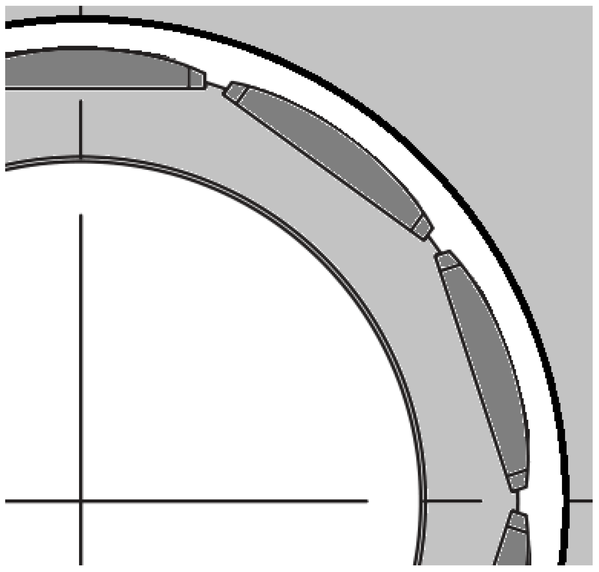
The oil friction loss of the motor is related to the oil flow pattern. Figure 9 is the partial enlarged detail of the axial view of the motor. The stator is encapsulated, and the inner surface is close to the smooth surface. Due to the periodic arrangement of permanent magnets, the outer surface of the rotor presents a groove shape. Therefore, the oil flow pattern in the gap is not a simple annular gap flow.

For the rotor with an uneven surface, the accurate flow of oil is usually obtained by finite element calculation. Suppose the rotor surface is smooth, that is, there is a smooth cylinder gap between the rotor and the stator. In fluid mechanics, the viscous fluid in the rotating cylindrical gap is defined as Taylor-Couette Flow. When the angular velocity is low, it can be known that the fluid is stable by measuring the Reynolds number. This state is called annular Couette flow. According to Couette’s research, the Reynolds number can be calculated by the following:

$$\mathrm{Re}=\omega R_i\left(R_a-R_i\right)/\upsilon$$

(6)

where $\mathrm{Re}$ is the Reynolds number; $\omega$ is the rotational angular velocity of the rotor; $R_a$ is the radius of the outer cylinder; $R_i$ is the radius of the inner cylinder; $\upsilon$ is the kinematic viscosity.

Taylor [20] proposed in the stability study of Couette flow that when the Reynolds number of the viscous fluid exceeds a certain critical value, the laminar flow pattern becomes unstable and enters the second stable state, that is, an axisymmetric annular vortex appears, which is called Taylor vortex. The critical Reynolds number of laminar instability can be calculated by Formula (7). Where P is the judgment condition of whether the oil state is unstable. Further, when $\delta /R_i$ is very small, the dimensionless Taylor number can be defined by Equation (8) [21].

$$\{\begin{array}{l}\mathrm{P}=0.0571\left(1-0.652\frac{\delta }{R_i}\right)+0.00056{\left(1-0.652\frac{\delta }{R_i}\right)}^{-1}\\ \mathrm{P}=\frac{{\pi }^4{\upsilon }^2\left(R_i+R_a\right)}{2{\omega }^2{\delta }^3{R}_i^2}\end{array}$$

(7)

$$\{\begin{array}{l}\sqrt{Ta}=\left(\omega R_i\delta /\upsilon \right)\sqrt{\delta /R_i}\\ \begin{array}{l}\hspace{1em}\delta =R_a-R_i\\ \hspace{1em}T{a}_c={\pi }^4/0.0571\approx 1706\end{array}\end{array}$$

(8)

when the Reynolds number continues to increase, the flow pattern of the viscous fluid will go through several stages such as Taylor traveling waves and modulated rotating waves, and then enter the turbulent state. Early scholars conducted a detailed experimental study on the flow pattern of Taylor-Couette flow at different Reynolds numbers. The experimental results and photos show that the critical Reynolds number of each stage is very dependent on the cylinder radius ratio $\eta =R_i/R_a$. Di Prima and Swinney [22] proposed an empirical formula for the torque applied on the inner cylinder when the viscous fluid was turbulent. The Taylor number in turbulent flow is about 12 times the critical Taylor number.

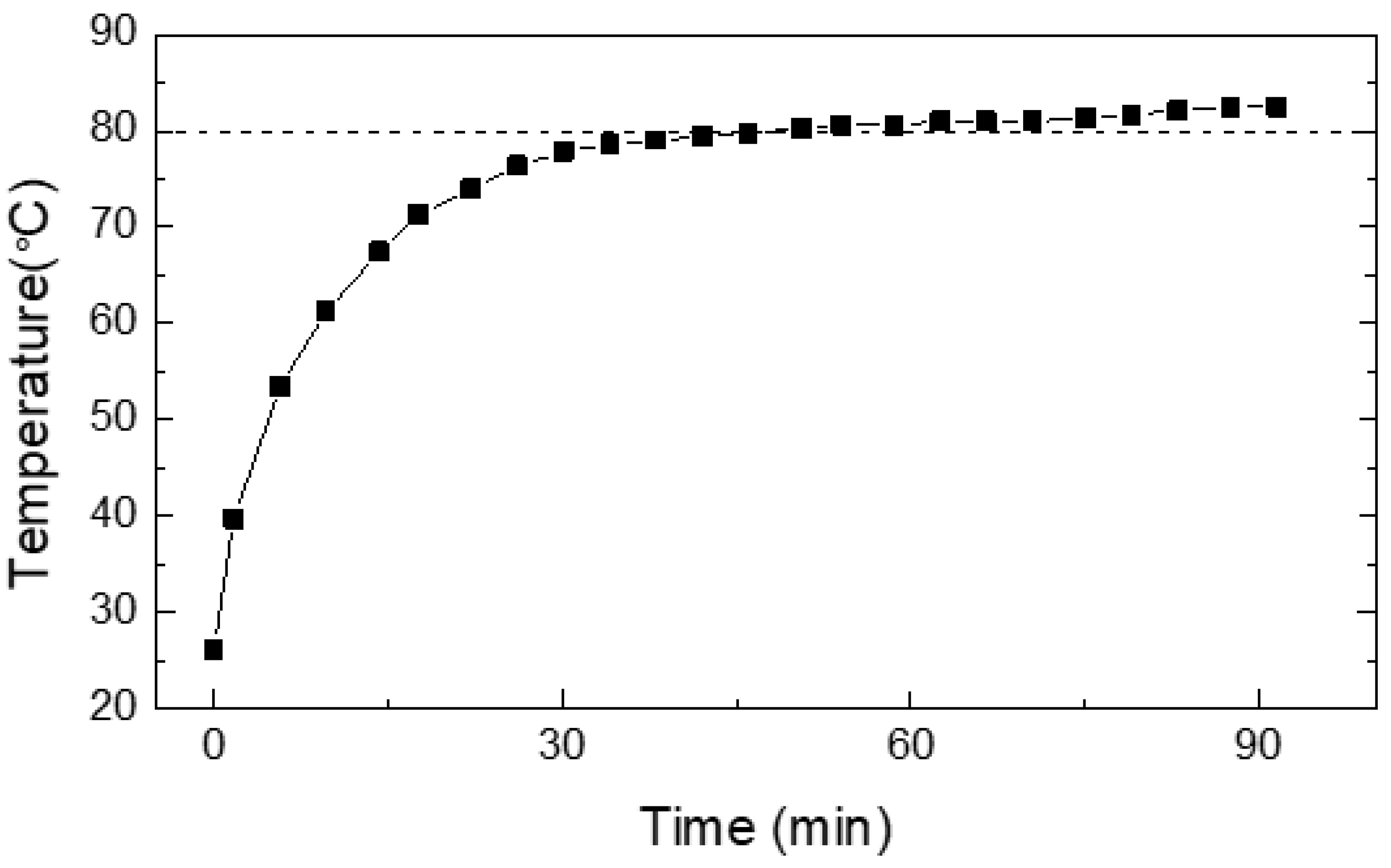
The temperature rise curve of the motor cylinder is shown in Figure 5, and the oil temperature gradually rises from 26 °C to 80 °C.

Table 4. Pressure-kinematic viscosity data of Mobil Velocite Oil NO.5 hydraulic oil (26 °C).

Pressure (MPa)	Compression Ratio (%)	Density (kg/m3)	Kinematic Viscosity (mm2/s)
0	0	850	12.34
20	97.65	870.46	15.38
30	96.55	880.37	17.10
40	96	885.42	19.07
50	95.48	890.24	21.22
60	94.93	895.40	23.55
80	93.65	907.63	28.73
100	92.75	916.44	34.86
115	91.65	927.44	39.90

is the pressure-kinematic viscosity data of No. 5 hydraulic oil at 26 °C. Taking the motor’s structure size into Equation (8), the motor speed range corresponding to different flow states can be obtained, as shown in

Table 5. Motor speed corresponds to different oil flow states in cylinder clearance.

Pressure (MPa)	Rotation Range (r/min)
	Laminar Flow	Transient Flow	Turbulent Flow
0	<149	149~1788	>1788
30	<201	201~2412	>2412
50	<248	248~2976	>2976
80	<339	339~4068	>4068
100	<419	419~5028	>5028
115	<489	489~5868	>5868

.

The rated speed of the motor is 2000 rpm. According to Table 5, at the rated speed, the oil in the motor gap is in the transient flow pattern. When the motor is at a lower speed, the friction torque can be calculated by Equation (9).

$$M_c=\mu \cdot {\left|\partial v/\partial r\right|}_{r=R_i}\cdot A=2\pi R_i^{2}h\mu {\left|\partial v/\partial r\right|}_{r=R_i}$$

(9)

In the laminar flow pattern, the velocity gradient is linearly distributed along the radial direction. When the viscous fluid is in the Taylor vortex state, Stuart calculated the characteristics of the flow pattern and obtained the calculation method of the velocity gradient. As shown in Equation (10), where $D=1.4472$ is a fixed value.

$${\left|\partial v/\partial r\right|}_{r=R_i}=\frac{\omega R_m}{\delta }\left[1+D\left(1-T{a}_c^2/T{a}^2\right)\right]$$

(10)

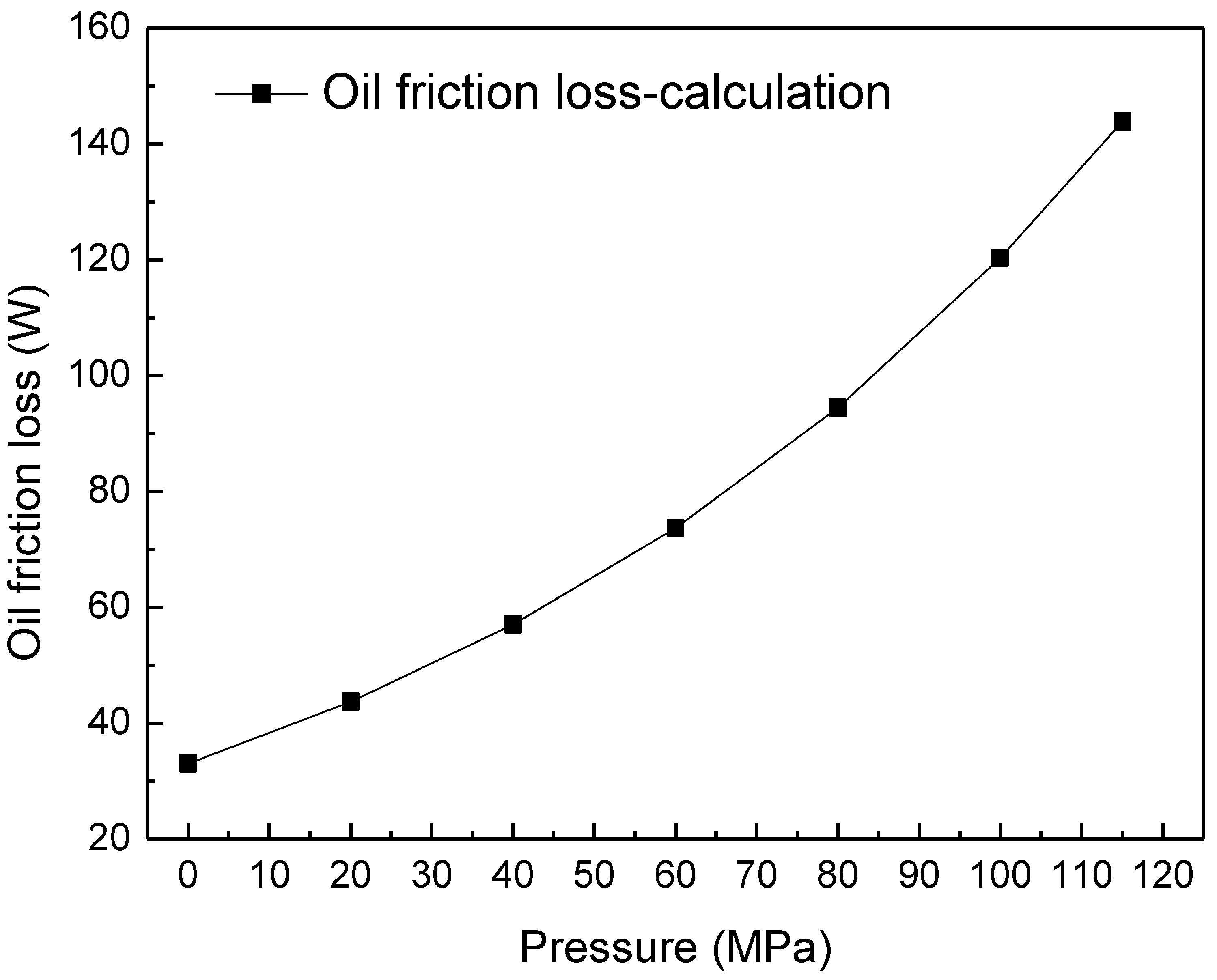
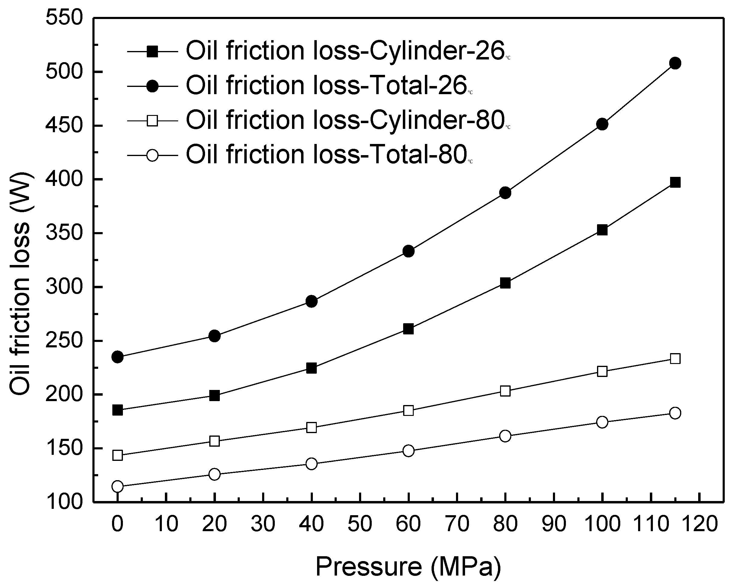
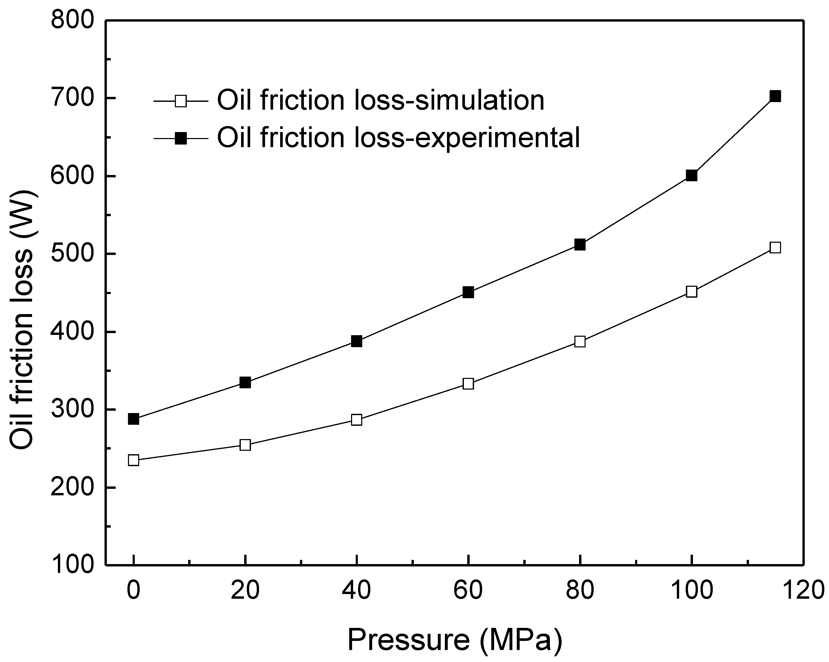
The friction torque on the smooth cylindrical surface can be calculated from the above equation. After determining the rotational speed of the rotor, the oil friction loss caused by viscous friction can be obtained. Bringing the motor structure size into the equation, the oil friction loss under different ambient pressures can be calculated, as shown in Figure 10. When the oil temperature remains constant, the oil friction loss of the inner rotor increases with the increase of the ambient pressure.

3.1.2. Simulation of Oil Friction Loss

The Taylor-Couette flow studies the annular gap between two rotating cylinders. For oil-immersed motors, the gap between the rotor end surface and the inner wall is also filled with hydraulic oil. Therefore, when calculating the oil friction loss of the motor, it is necessary to calculate the total friction torque of the cylinder surface and the two end surfaces.

The simplified motor is modeled by the finite element simulation software ANSYS Workbench. The inner surface of the motor is simplified into two coaxial cylinders of different sizes, and the calculated flow field is the closed area formed by the two cylindrical surfaces. Since there is no oil exchange with the valve box, there is no inlet and outlet for the flow field in the model.

The flow field was meshed using the “Tetrahedrons” tetrahedral meshing method. Since the model is a simple geometry, the “Patch Conforming” mesh mapping method based on the “TGRID” algorithm is used to generate the volume mesh from the surface mesh. The mesh encryption scheme is shown in

Table 6. Mesh Refinement Scheme for Simplified Models.

	First Layer (mm)	Growth Rate	Elements
1	0.2	1.2	1,946,995
2	0.15	1.2	2,093,535
3	0.1	1.2	2,404,342
4	0.1	1.1	2,972,813
5	0.08	1.1	3,240,947
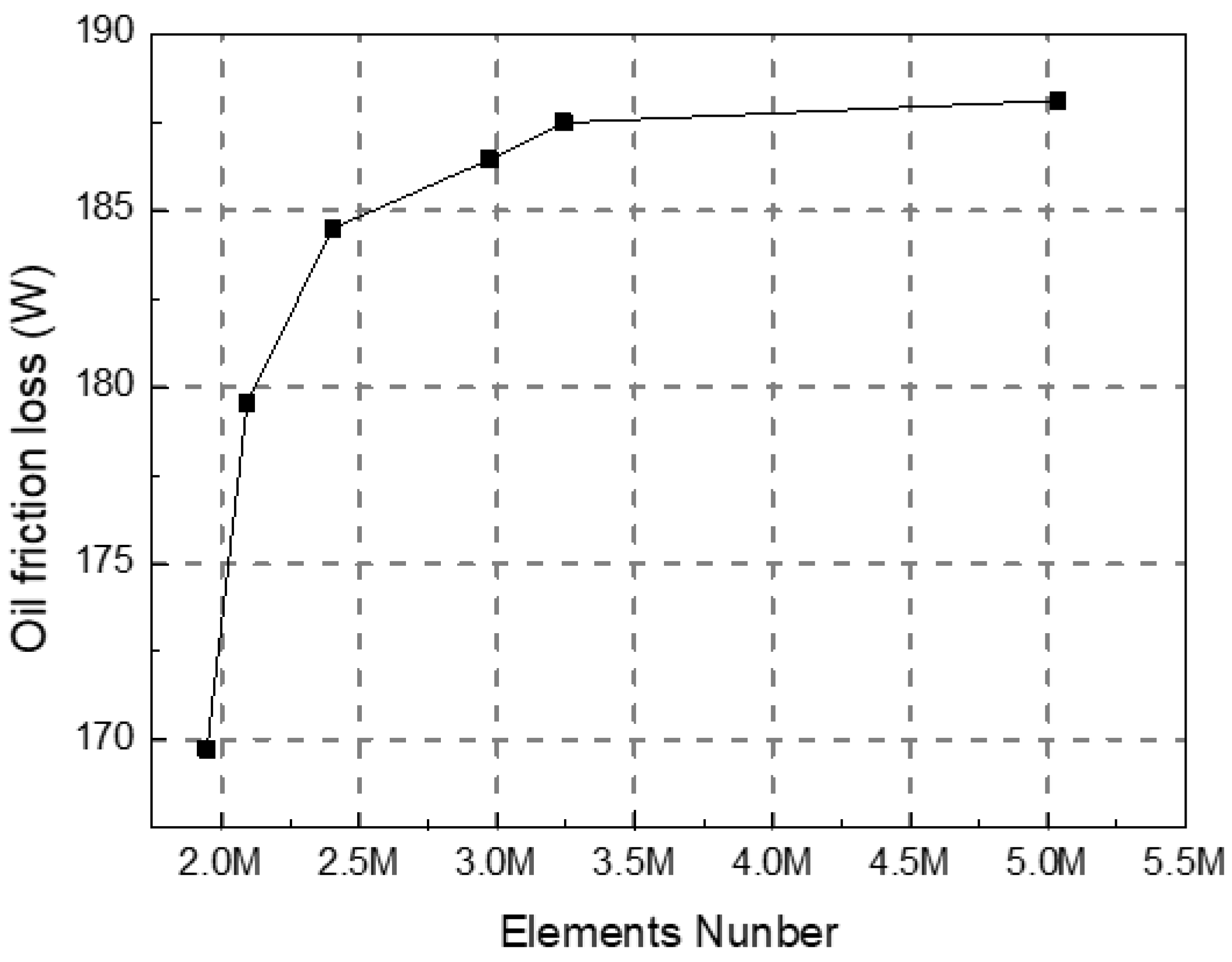
6	0.08	1	5,035,864

. The “Inflation” refinement method was applied to the flow field within a cylindrical gap of approximately 2 mm. The oil friction loss calculated by different mesh refinement models is shown in Figure 11. When the mesh number exceeds 3.3 M, the variation rate of simulation results is about 0.5%. Therefore, simulations were performed using the fifth set of mesh refinement schemes.

Import the mesh data into CFX, and set the material properties according to the pressure-viscosity data calculated above. Fixed the outer surface, applied rotation speed of 2000 rpm on the inner surface. The “Shear Stress Transport” turbulence model was selected to calculate the friction torque of the inner rotor under different oil viscosity conditions.

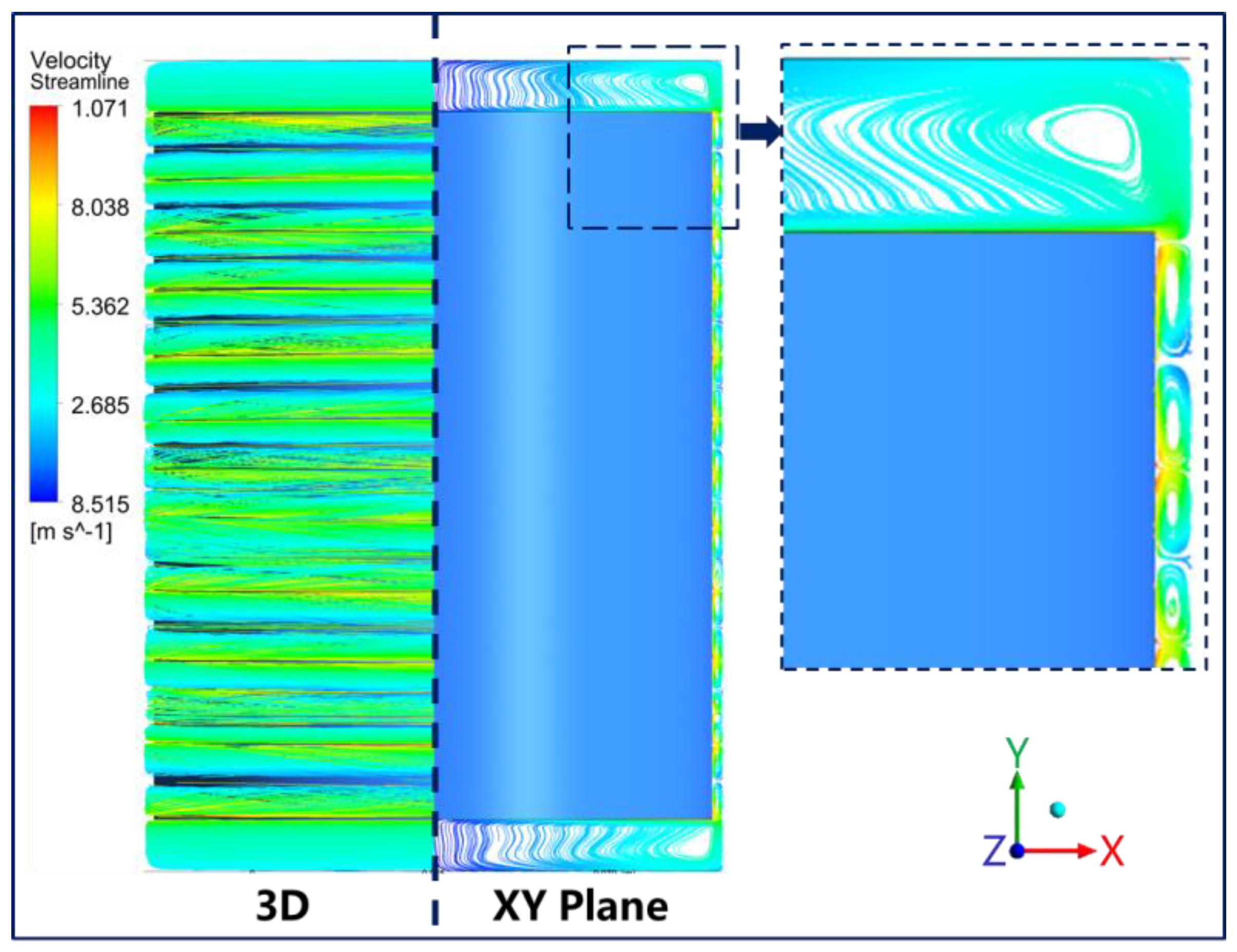
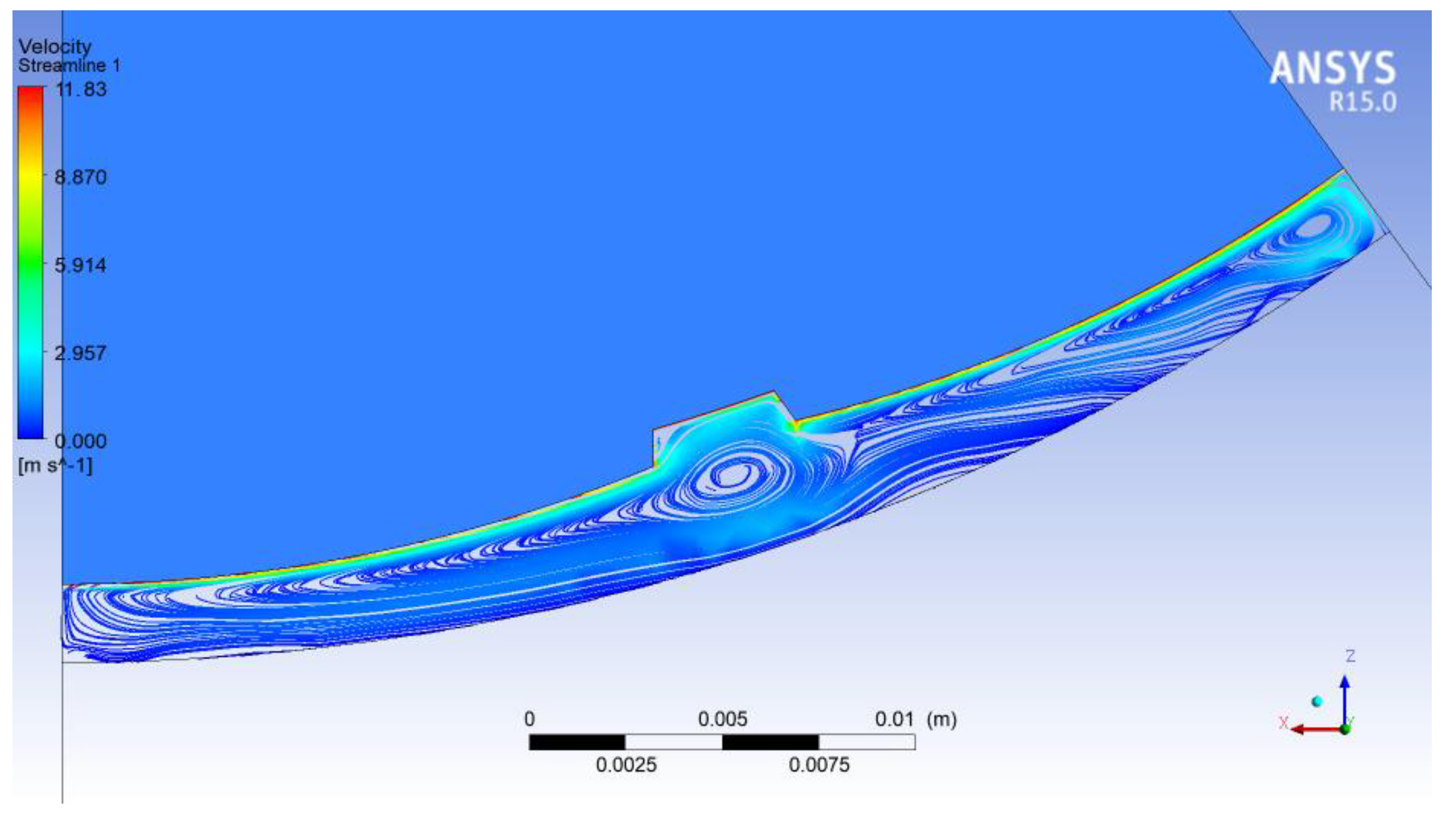
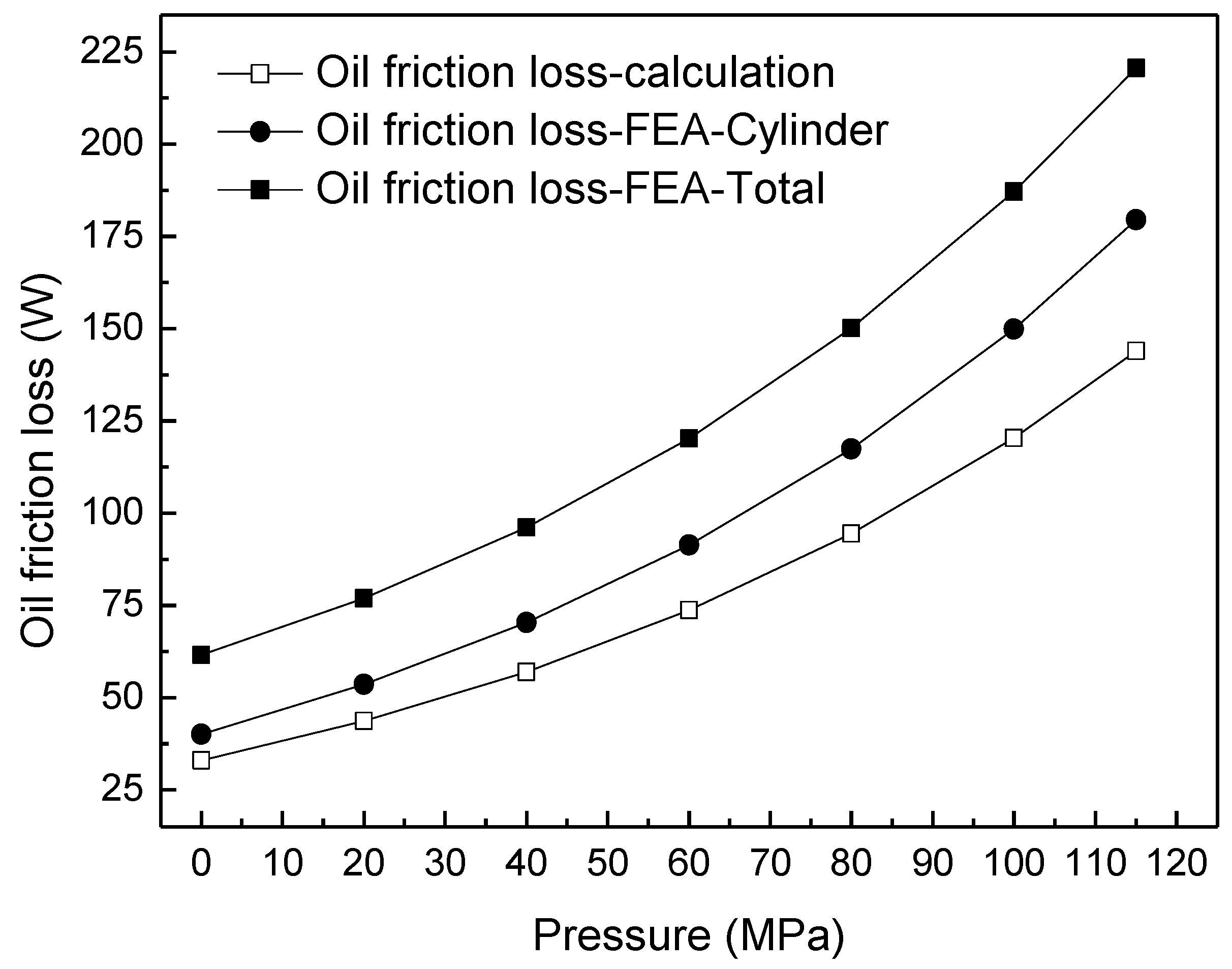
The simulation results are shown in Figure 12. Taking the simulation results when the ambient pressure is 100 MPa as an example, the flow field in the cylindrical gap is in the state of transient flow, which presents a periodic vortex. The left side of Figure 12 is the 3D flow field obtained from the simulation, and the right side is the surface streamline on the XY cross-section and a partial enlarged view. It can be seen from the enlarged figure that under the effect of centrifugal force, the flow field on the end surface is in turbulent state, and a small part of it invades the cylindrical gap. The torque of each rotor surface along the Y axis was read through CFX-post, and the oil friction loss of each surface was calculated, as shown in Figure 13. The three curves represent: the theoretical values calculated by Equation (9), the simulation values of the cylindrical surface and the entire rotor surface simulated by the CFX. Affected by the flow field on the upper and lower end faces of the rotor, the oil friction loss on the cylindrical surface is slightly larger than the theoretical calculation result.

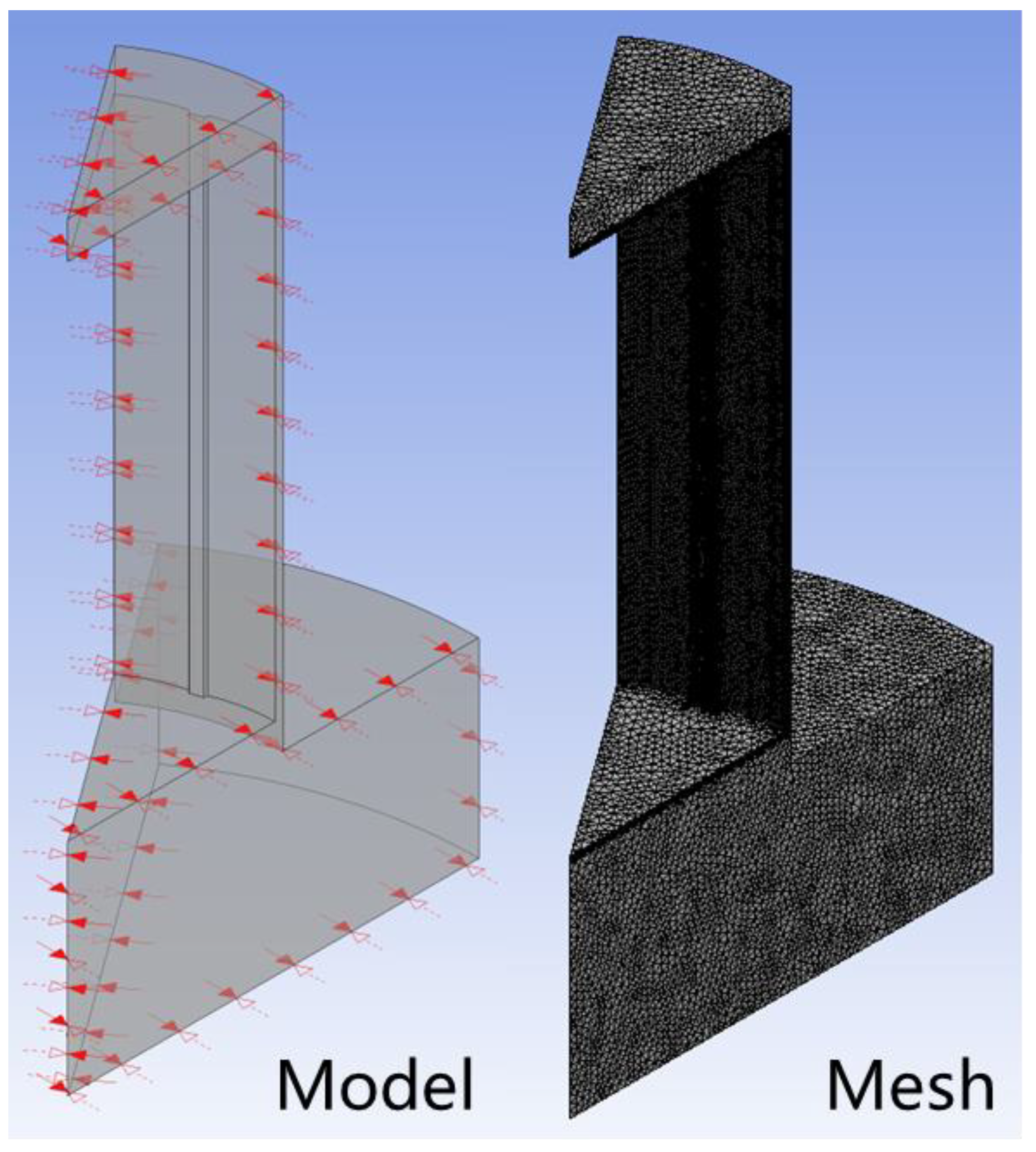
Further, the actual motor rotor model is simulated. The actual motor rotor consists of 10 groups of uniformly distributed permanent magnets. In order to reduce the computing time and improve the quality of the mesh, a partial model of the motor is established.

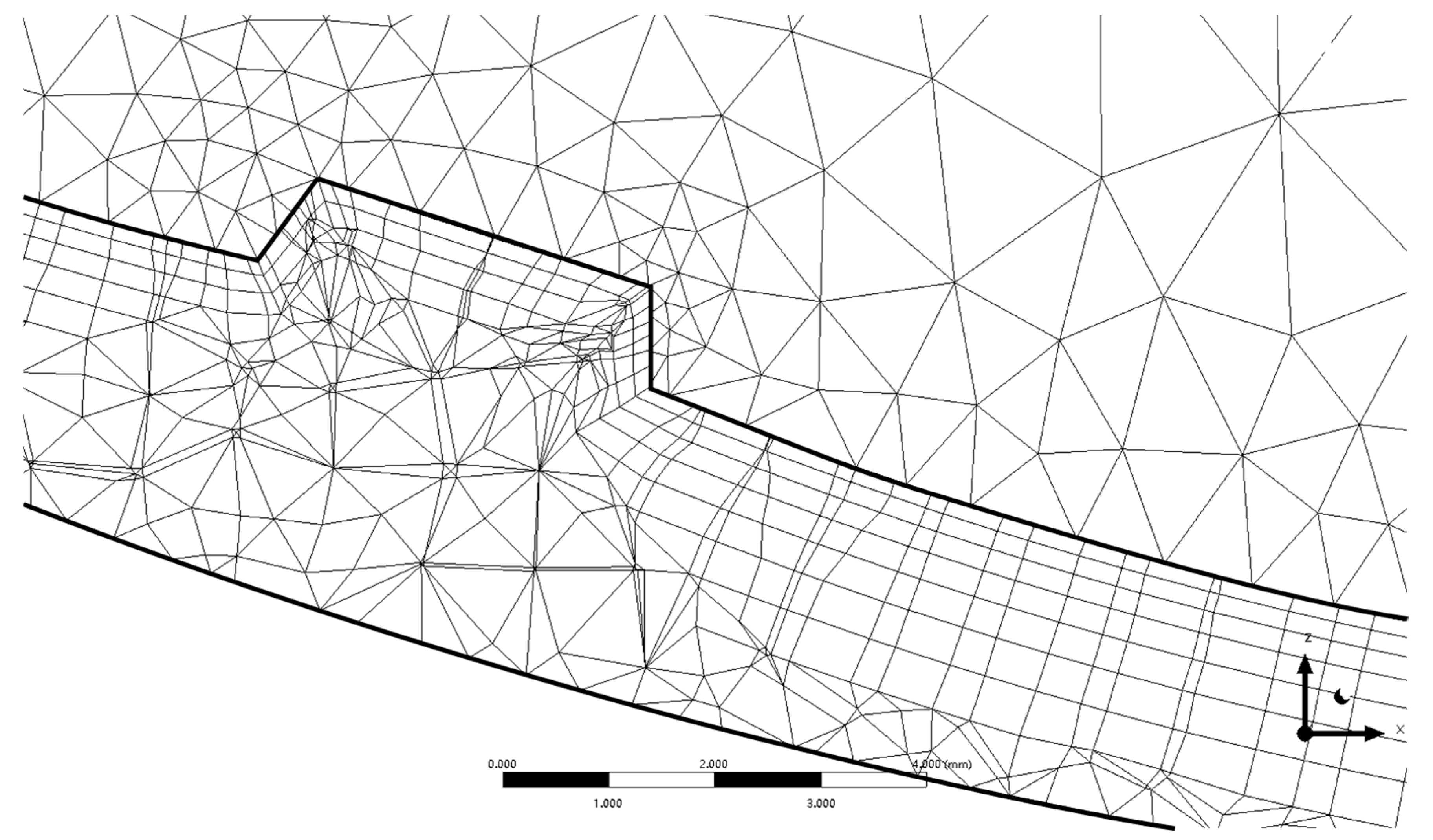
The flow field was also meshed using the “Tetrahedrons” tetrahedral meshing method. Due to the complexity of the model, the “Patch Conforming” mesh mapping method based on the “ICEM CFD Tetra” algorithm is used to generate the surface mesh from the volume mesh. The meshing results are shown in Figure 14, and Figure 15 shows the cross-section perpendicular to the Y axis. The mesh encryption scheme is shown in

Table 7. Mesh Refinement Scheme for Detailed Models.

	First Layer (mm)	Growth Rate	Elements
1	0.15	1.2	672,591
2	0.1	1.2	723,055
3	0.1	1.1	775,224
4	0.1	1	827,635
5	0.08	1.1	977,230
6	0.08	1	1,092,380
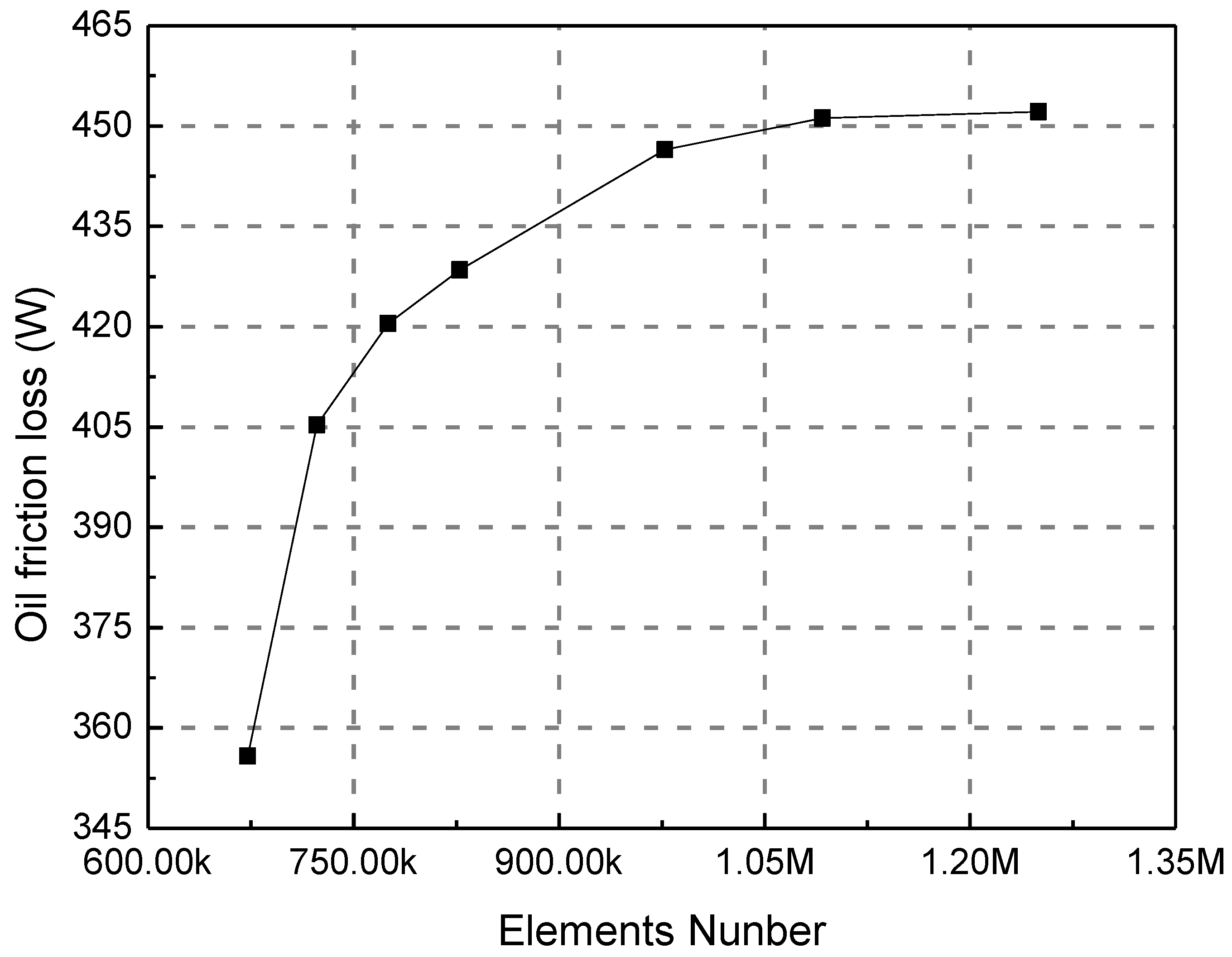
7	0.06	1	1,249,870

. The oil friction loss calculated by different mesh refinement models is shown in Figure 16. When the mesh number exceeds 1.1 M, the variation rate of simulation results is about 0.5%. Therefore, simulations were performed using the sixth group of mesh refinement schemes.

The simulation parameters are the same as before, using the “Shear Stress Transport” turbulence model and applying “Symmetry” on the cross section of the flow field. The simulation results are shown in Figure 17. Affected by the groove, there is no periodic eddy current in the annular gap, and the viscous fluid moves irregularly in the radial direction. The oil flow pattern at this time conforms to the characteristics of turbulent flow, that is, the groove has a great influence on the oil flow pattern in the cylindrical gap.

Specifically, the curve of motor oil friction loss with ambient pressure is shown in Figure 18. As the ambient pressure increases, the oil friction loss of the motor increases gradually. That is, when driving the same load, the overall efficiency of the motor is gradually reduced.

Compared with the simulation results of the simplified model, under the same oil temperature, the oil friction loss of the detailed model increases significantly. It means that the grooves on the rotor surface will disturb the flow field and also have a great influence on the oil friction loss. Comparing the simulation results at different temperatures, when the oil temperature increases, the oil friction loss decreases. Therefore, the temperature in the motor barrel can be appropriately increased to reduce the oil friction torque, and improve the efficiency of the oil-filled motor.

3.2. Pump Efficiency

The pressure compensator balances the internal pressure and the ambient pressure, so the commercially available hydraulic component can work normally in the deep sea high pressure environment. However, as the ambient pressure increases, the fluid properties change. When the hydraulic pump squeezes the oil and converts the mechanical energy into hydraulic energy, the change of the oil characteristics will directly affect the working characteristics of the pump.

In this paper, the external gear pump is selected, which is a positive displacement pump. It has a simple structure and high reliability, and is suitable for working in a complex environment. However, compared with piston pump, vane pump, etc., the internal leakage is relatively large. Therefore, when the load pressure is consistent, the efficiency of the gear pump is affected by both the hydro-mechanical efficiency ${\eta }_{hm}$ and the volumetric efficiency ${\eta }_V$. The specific pump efficiency can be expressed as:

$$\{\begin{array}{l}{P}_{pump}=P_{hm}+P_V+P_{out}\\ {\eta }_{pump}=P_{out}/P_{pump}={\eta }_V\times {\eta }_{hm}\end{array}$$

(11)

where, $P_{pump}$ is the mechanical energy input from the motor; $P_{hm}$ is the hydraulic-mechanical power loss; $P_V$ is the power loss caused by oil leakage; $P_{out}$ is the output power of pump.

(1) Volumetric efficiency

The internal flow loss of the gear pump mainly comes from the gear end clearance, radial clearance and gear meshing. The volumetric efficiency of a gear pump can be expressed by the following equation:

$${\eta }_V=\frac{q_P}{q_s}=\frac{q_P}{q_P+q_{loss}}=\frac{q_s-q_{loss}}{q_s}$$

(12)

where, $q_s$ is the theoretical flow, which equals to the rated displacement times rotational speed; $q_P$ is the output flow of the pump outlet; $q_{loss}$ is the internal leakage flow.

The leakage flow from the end surface clearance accounts for about 80% of the total, and can be calculated by Equation (13).

$$Q_l=\frac{\pi s^3\Delta p}{6\mu \ln (R_1/R_2)}\times \frac{\theta }{2\pi }\times 60\times {10}^3=\frac{\theta s^3\Delta p}{2\mu \ln (R_1/R_2)}\times {10}^4$$

(13)

In Equation (13), end surface clearance s, dedendum circle radius $R_1$, gear shaft radius $R_2$ are the structural dimensions of the gear pump, and the pressure difference $\Delta p$ between the high pressure chamber and the bearing chamber is determined by the actual load condition. Therefore, when the load pressure is consistent, the leakage from the high pressure chamber is negatively correlated with the dynamic viscosity of oil. That is, when the ambient pressure increases, the internal leakage of gear pump will decrease.

(2) Hydro-mechanical efficiency

Friction loss of gear pump mainly includes mechanical friction between the pump shaft and bearing, and viscous friction between the gear and oil. In good lubrication, mechanical friction can be ignored compared with viscous friction. Hydraulic—mechanical efficiency of gear pumps can be expressed as follows:

$${\eta }_{hm}=\frac{P_{pump}-\Delta P_{hm}}{P_{pump}}=\frac{T_{pump}-\Delta T_{hm}}{T_{pump}}=\frac{p_P}{p_P+\Delta p_{hm}}$$

(14)

where, $\Delta P_{hm}$ is the frictional power loss, $T_{pump}$ is the input torque of the gear pump, $\Delta T_{hm}$ is the torque loss due to friction, and $\Delta p_{hm}$ is the corresponding pressure value calculated from the lost torque.

The viscous friction loss of the gear pump mainly includes: the viscous friction loss between addendum circle and the oil, and between gear end face and the oil. According to Newton’s viscous fluid friction law [23], the frictional shear stress τ on the contact surface between gear and oil can be calculated by Equation (15).

$$\tau =\mu {\left(\frac{\partial u}{\partial y}\right)}_{y=0}$$

(15)

where, $u$ is the oil velocity relative to the contact surface; $\partial u/\partial y$ is the oil velocity gradient in the normal direction of the contact surface.

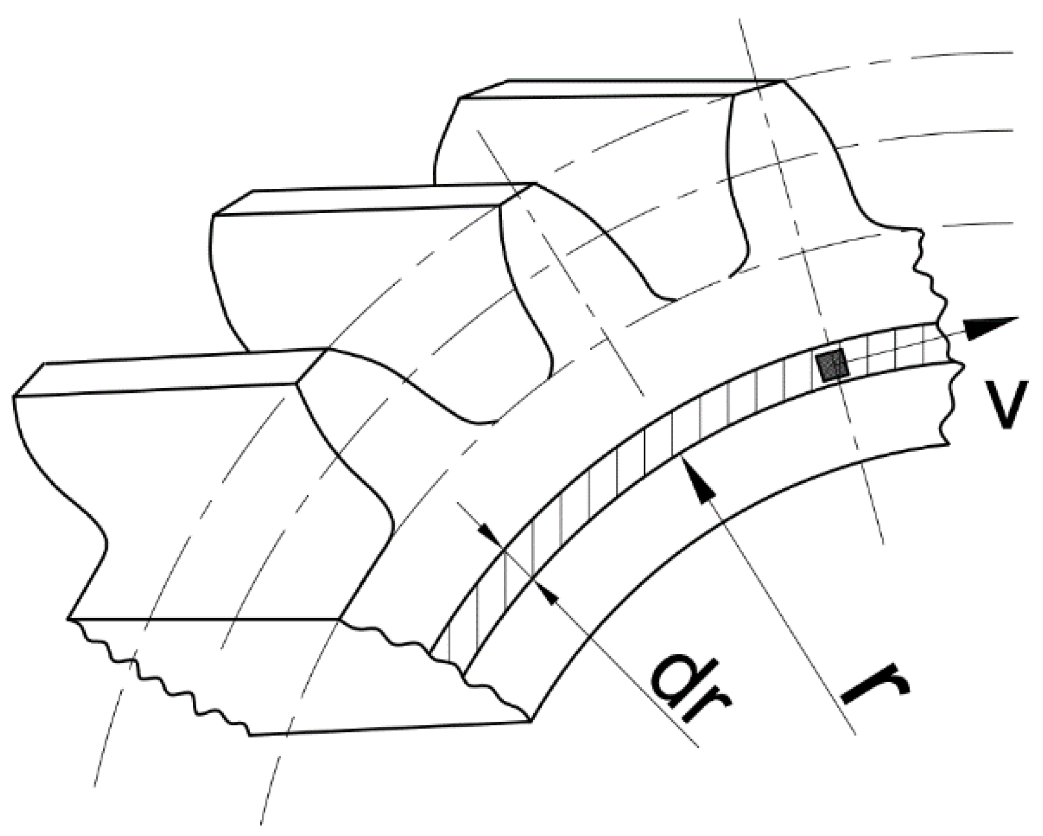
The frictional shear stress on the end face of the addendum circle and the side face of the gear is theoretically deduced, and the hydro-mechanical loss of the gear pump can be further obtained, that is, Equation (16).

$$\begin{array}{ll}\Delta P_{hm}& =2\Delta N_{radial}+4\Delta N_{axial}\\ & =2{\displaystyle \int {\tau }_{radial}dAv}+4{\displaystyle \int {\tau }_{axial}dAv}\end{array}$$

(16)

where, $\mu$ is the dynamic viscosity of the oil; $\Delta N_{radial}$ is the viscous friction loss on the addendum circle surface; $\Delta N_{axial}$ is the viscous friction loss on the gear’s side surface; $A$ is the area of the contact surface, and $v$ is the linear velocity. Taking Figure 19 as an example, on the side surface of the gear, $dA=2\pi rdr$; $v=2\pi nr/60$.

According to the derived Equations (12)–(16), it can be known that in the deep-sea high-pressure environment, with the increase of oil viscosity, the internal leakage flow of the pump decreases, and the frictional power loss increases. The volumetric efficiency and mechanical efficiency of the pump have opposite trends. Therefore, it is necessary to bring in the actual structural data to obtain the specific variation curve of the gear pump efficiency.

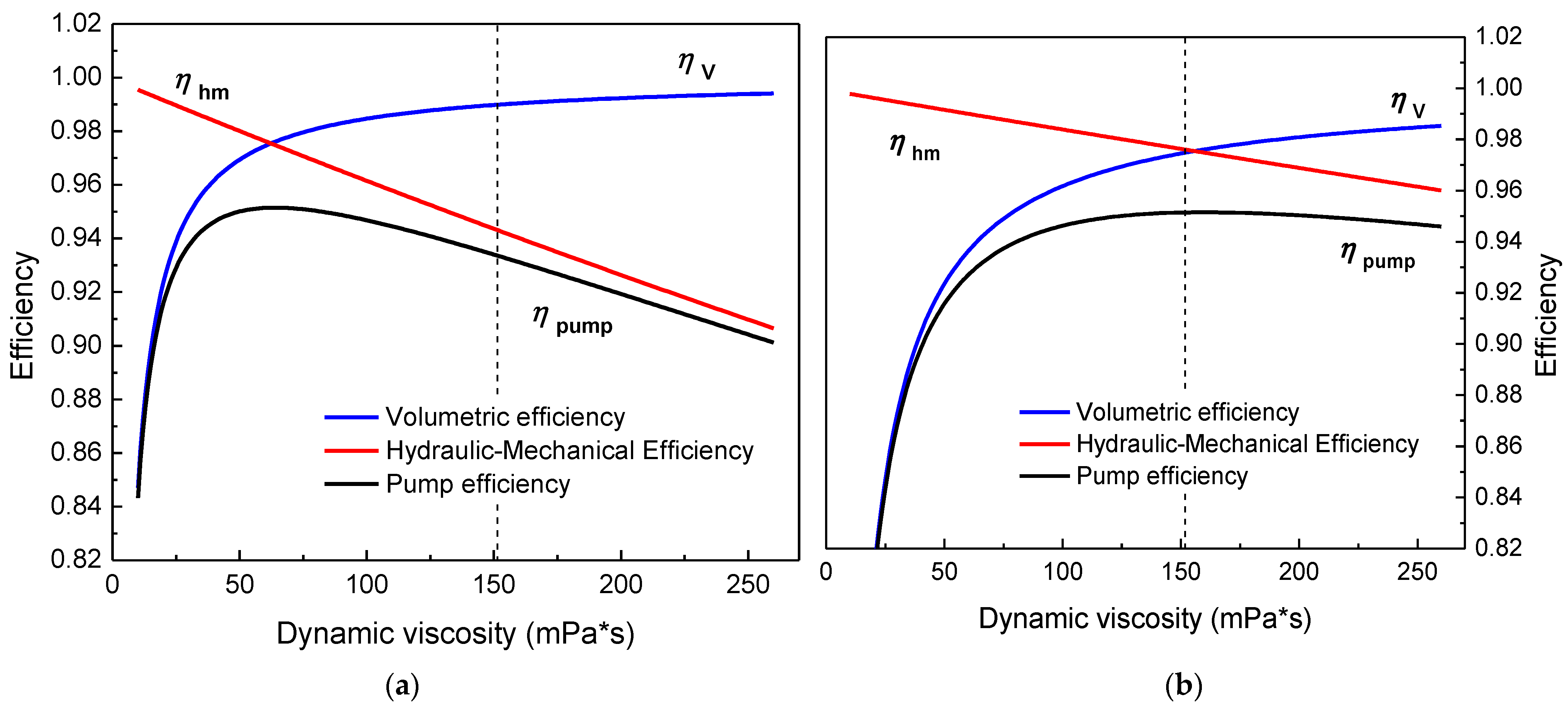
The gear pump selected in this article is Rexroth’s AZPF external gear pump, with a rated displacement of 8.0 cm³/rev. The load conditions are assumed to be the same, that is, the pump output pressure $p_P$ remains the same. Bring in structural data, and the volumetric efficiency and mechanical efficiency as a function of oil viscosity were calculated. The variation curves of pump efficiency when the motor speed is 2000 rpm and the load pressure are 6 MPa and 15 MPa respectively are calculated, as shown in Figure 20.

It can be seen from Figure 20 that when the load pressure is consistent, the hydraulic mechanical efficiency decreases approximately linearly with the increase of the oil viscosity. For the volumetric efficiency of the gear pump, as the oil viscosity increases, the volumetric efficiency first increases rapidly, and then slowly approaches 1. That is, when the oil viscosity is low, the internal leakage flow of the gear pump is more sensitive to the change of oil viscosity.

The variation curve of gear pump efficiency can be obtained by Equation (11): with the increase of oil viscosity, the pump efficiency first increases and then gradually decreases. Analyze the reason: (1) when the oil viscosity is low, the viscous frictional resistance of the gear is almost negligible relative to the input torque of the pump. At the same time, the rapid decrease of the internal leakage flow makes the overall efficiency of the pump continue to increase. (2) As the oil viscosity continues to increase, the decreasing rate of internal leakage flow slows down and stabilizes at a lower level. The viscous frictional resistance of gears continues to increase and has an increasing impact on pump efficiency. When the changing rate of the volumetric efficiency is less than that of the hydraulic-mechanical efficiency, the pump efficiency curve has a turning point.

The dotted line in Figure 20 corresponds to a viscosity value of 152 MPa·s. It represents the viscosity of Nuto H10 hydraulic oil at 32 °C when the ambient pressure is 115 MPa. Taking the hydraulic mechanism carried on “Jiaolong” as an example [18], when the manned submersible is in operation and attitude adjustment, the pressure requirement of the load actuator is 15–19 MPa. In the floating and diving process of manned submersible, the pressure requirement of the de-ballasting cylinder is about 6 MPa. Therefore, in most of the operation process, the efficiency of the pump in the deep-sea hydraulic source prototype gradually increases with the ambient pressure.

3.3. Hydraulic Efficiency

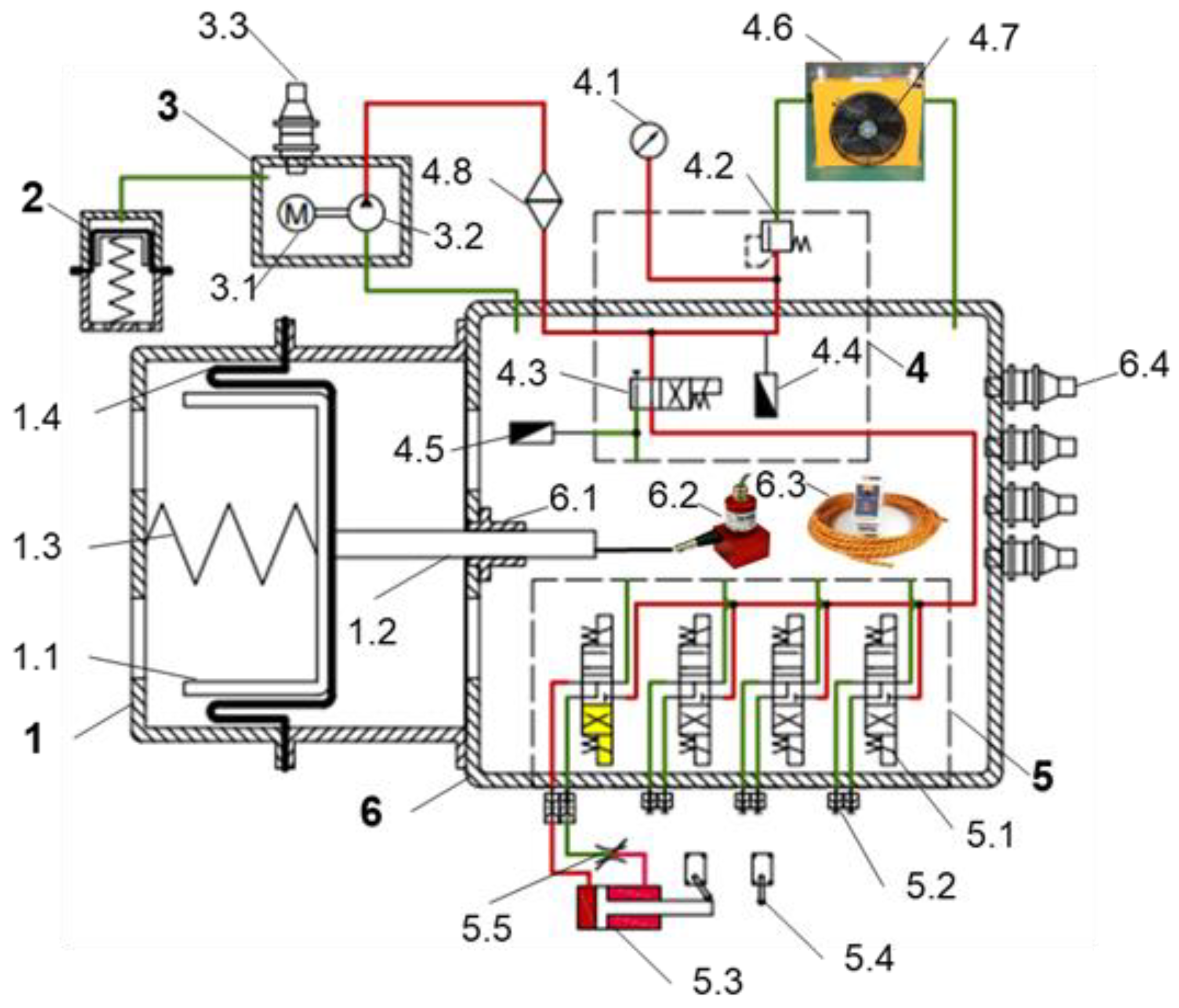
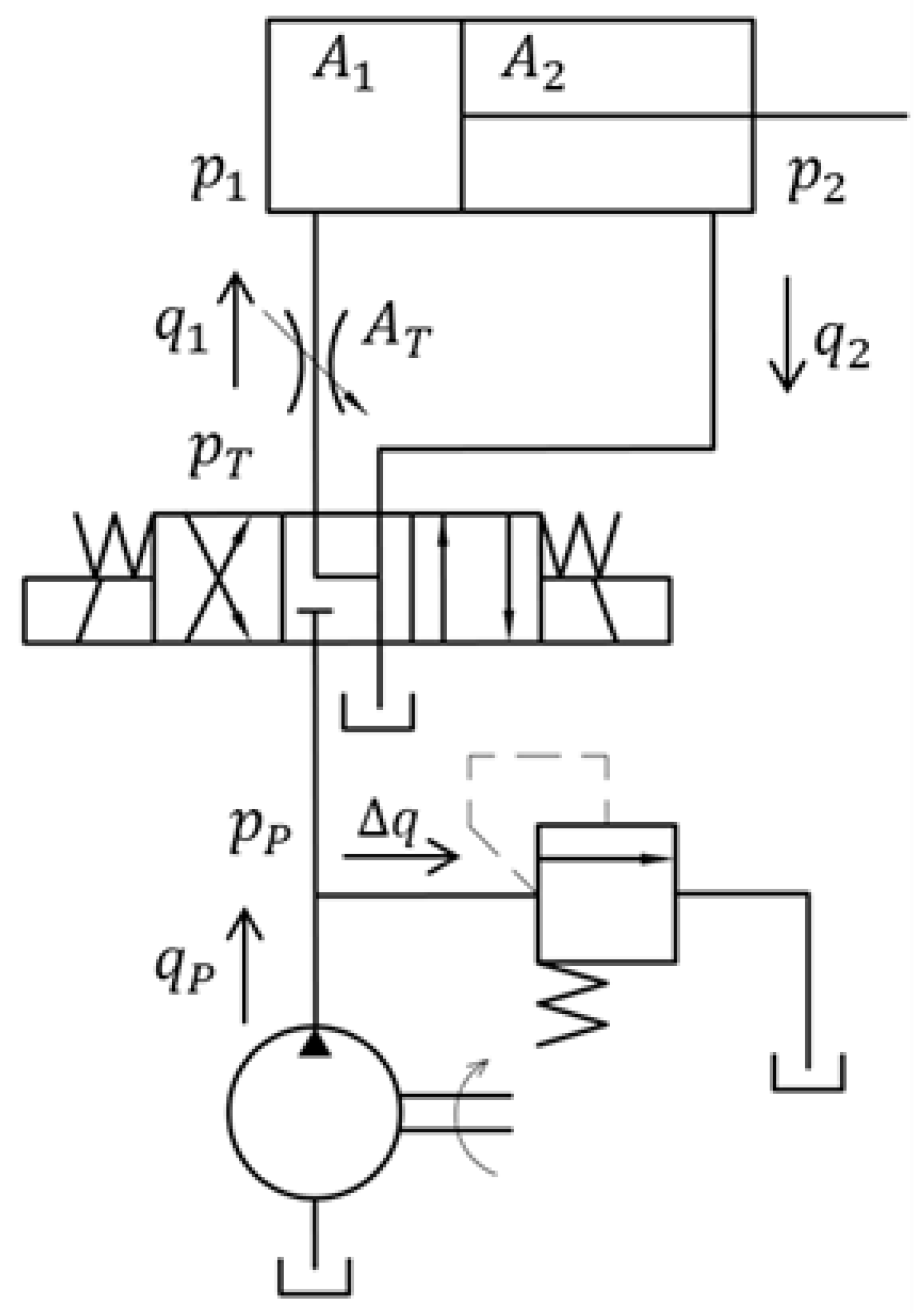
The load actuator of the deep-sea hydraulic source system is mainly the hydraulic manipulator. This paper mainly studies the working characteristics of the deep-sea hydraulic source prototype, so the load unit is simplified as a single-rod hydraulic cylinder controlled by the solenoid directional valve. A simplified hydraulic circuit schematic is shown in Figure 21.

To simulate different load situations, a throttle valve is connected in series with the single-rod hydraulic cylinder. When the motor speed is constant, different load conditions can be simulated by setting different throttle valve openings. The relief valve is used to adjust the maximum working pressure of the hydraulic system. The efficiency of the hydraulic circuit can be expressed as:

$$\{\begin{array}{c}{\eta }_{hydr}=\frac{p_T{q}_1}{p_p{q}_p}=\frac{p_T{q}_1}{\left(p_T+p_{loss}\right)\left(q_1+\Delta q\right)}\\ q_1=C_d{A}_T\sqrt{\frac{2\left(p_T-p_1\right)}{\rho }}\end{array}$$

(17)

where, $q_1$ is the load flow; $p_T$ is the inlet pressure of the throttle valve; $p_1$ and $p_2$ is the pressure of rear end chamber and rod end chamber; $A_1$ and $A_2$ is the effective working area of rear end chamber and rod end chamber; $A_T$ is the flow cross-section area of the throttle valve; $p_{loss}$ is the pressure loss of the circuit; $\Delta q$ is the overflow rate.

During the prototype test, no additional load was applied to the hydraulic cylinder rod. When the output pressure of the pump does not reach the opening pressure of the relief valve, it can be approximated as q_P ≈ q₁. The efficiency of the hydraulic circuit can be approximately equivalent to the ratio of the load pressure to the pump output pressure.

Due to the energy loss of the viscous oil moving in the pipeline, the load pressure is lower than the pump’s output pressure. Among them, the main reasons for the pressure loss are: (1) When the oil flows in the pipeline of equal diameter, the friction head loss caused by the viscous friction. (2) When the oil flows through the suddenly changing section, such as elbows and joints, the local pressure loss caused by the change of flow velocity or flow direction.

(1) Friction head loss

The friction head loss is mainly affected by the roughness of the pipe wall and the fluid flow state, which can be expressed as:

$$\{\begin{array}{l}\Delta p_{\lambda }=\lambda \frac{l}{d}\frac{\rho U^2}{2}\\ \lambda =f\left(\mathrm{Re},\Delta /d\right)\end{array}$$

(18)

where, Δ is the surface roughness of the pipe wall; $d$ is the inner diameter of the pipe; $l$ is the length of the pipeline; $\lambda$ is the frictional resistance coefficient; $\rho$ is the oil density, and $U$ is the average flow rate.

Equation (18) is suitable for the calculation of the friction head loss when the fluid is in laminar state and turbulent state. When the fluid is in the laminar state, the friction resistance coefficient is only related to the Reynolds number Re. At this time, the theoretical value of the friction resistance coefficient is $\lambda =64/\mathrm{Re}$. Considering that the temperature may fluctuate during the actual flow, when the liquid flows in the metal pipe, $\lambda =75/\mathrm{Re}$. When the liquid flows in the rubber pipe, $\lambda =80/\mathrm{Re}$.

The inner diameter of the pipeline used in the hydraulic source system is 6 mm. Assuming that the pump’s output flow is the theoretical value of 16 L/min, the dynamic viscosity value of Nuto H10 hydraulic oil is brought into Equation (19), and the Reynolds number of oil flow under different ambient pressures is obtained, as shown in

Table 8. Reynolds number of oil in pipeline under different ambient pressure.

pAmbient (MPa)	0.1	20	30	40	60	80	100	115
Re	3698	2543	2108	1738	1181	804	545	409

.

$$\mathrm{Re}=\frac{Ud}{\upsilon }$$

(19)

The critical Reynolds number for judging the laminar flow in a circular tube is Re ≤ 2320. It can be seen from Table 8 that in the deep-sea environment with a depth over 2000 m, the flow in the pipeline is in the laminar state. The length of the pipeline in the prototype is about 1.5 m, so when the ambient pressure is 115 MPa, the pressure loss along the metal pipe is:

$$\Delta p_{\lambda }=\frac{75}{\mathrm{Re}}\frac{l}{d}\frac{\rho v^2}{2}=\frac{75\times 1.5\times 927.44\times {10}^{-6}\times {9.43}^2}{409\times 0.006\times 2}=1.89 \mathrm{MPa}$$

(20)

(2) Local pressure loss

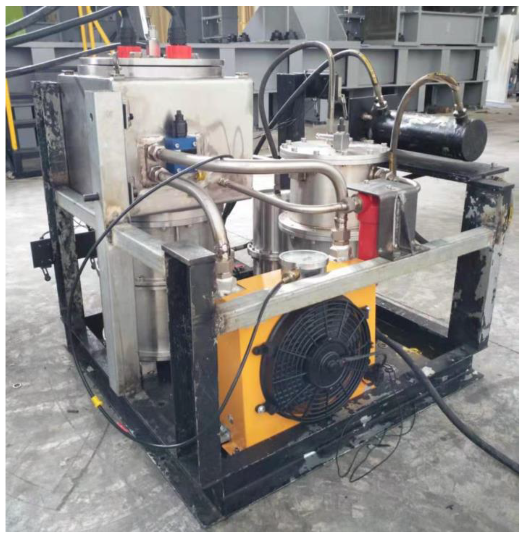
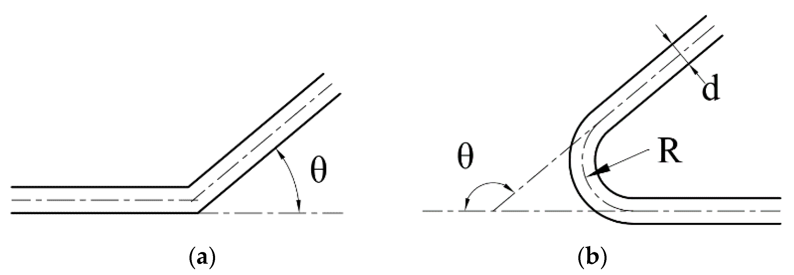
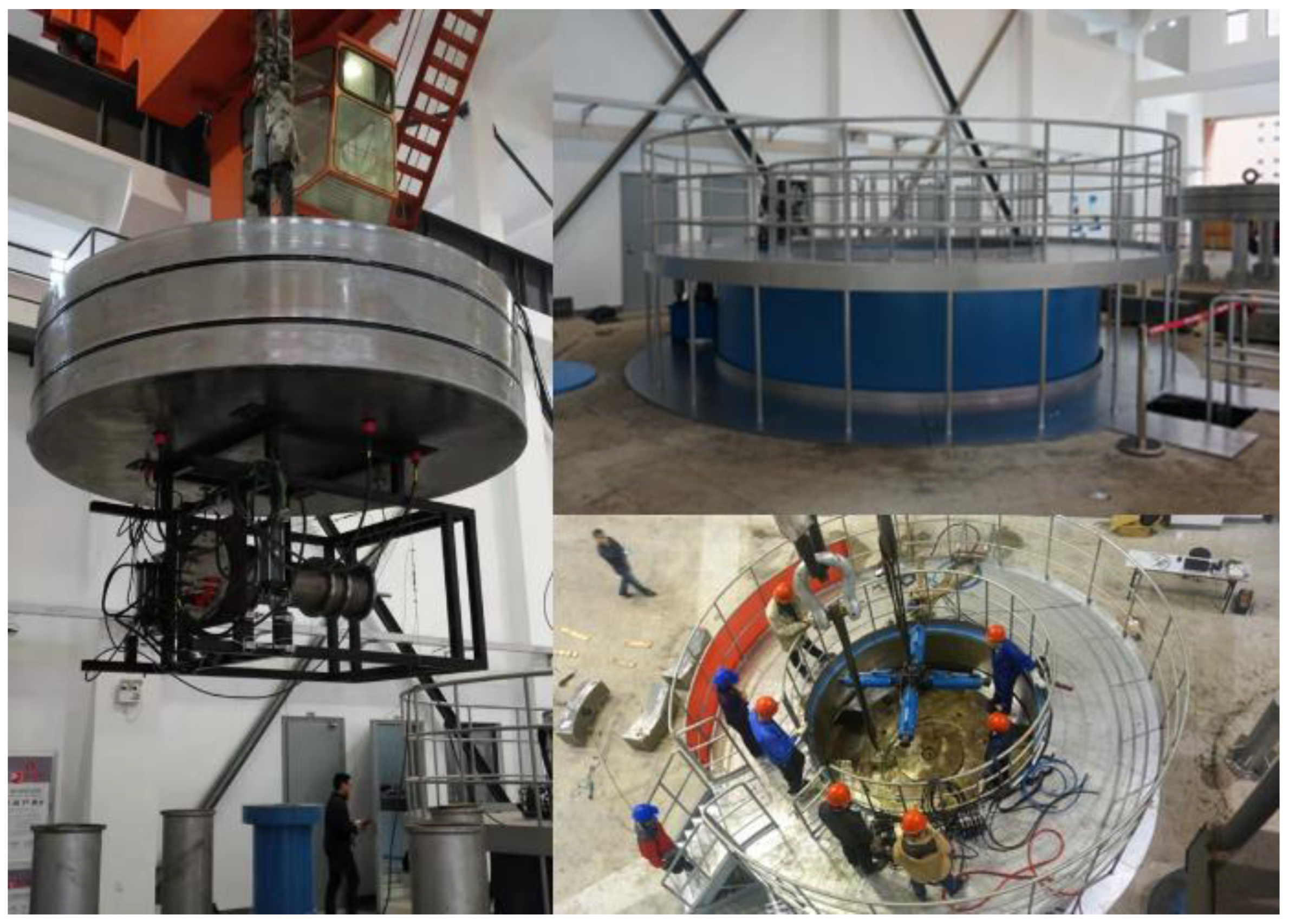
The local pressure loss mainly includes the resistance loss at the elbow and the variable section. As shown in Figure 2, the main pipeline of the hydraulic source prototype is made of seamless steel pipes. Use only hydraulic hoses to connect the load throttle and hydraulic cylinder. The use of welded pipe joints ensures that the inner diameter of the main pipeline is uniform and reduces the local pressure loss at the variable section. There are two types of elbows that change the flow direction in the hydraulic circuit, as shown in Figure 22.

The flow phenomenon in the elbow is very complex, and the pressure loss coefficient is generally determined by experiments. The general expression for the local pressure loss is:

$$\Delta p_{\zeta }=\zeta \frac{\rho U^2}{2}$$

(21)

where, $\zeta$ is the local resistance coefficient and $U$ is the average flow velocity.

The calculation equation of the local resistance coefficient is shown in

Table 9. Calculation of the local resistance coefficient and pressure loss.

Type	Coefficient Formula	Result	Amount
Miter bend pipe (a)	${\zeta }_a=0.946{\sin }^2\left(\frac{\theta }{2}\right)+2.05{\sin }^4\left(\frac{\theta }{2}\right)$	0.985	5
Smooth bend pipe (b)	${\zeta }_b\text{=}\left[0.131\text{+}0.163{\left(\frac{d}{R}\right)}^{3.5}\right]\frac{2\theta }{\pi }$	0.13	8

. Where, $\theta$ is the direction change angle of the elbow, $d$ is the inner diameter of the bend pipe, and $R$ is the radius of curvature of the elbow. In the hydraulic source prototype, the bend angles are all 90°. The average radius of curvature of the metal pipe is 30 mm, $d/R=0.2$.

Miter bend pipes mainly exist in valve blocks, valves and other accessories, and smooth bend pipes mainly exist in metal pipes, elbows and other accessories. Substituting the data in Table 9 into Equation (21), the local pressure loss when the ambient pressure is 115 MPa can be obtained:

$$\Delta p_{\zeta }=\left(5{\zeta }_a+8{\zeta }_b\right)\frac{\rho U^2}{2}=5.965\times \frac{927.44\times {10}^{-6}\times {9.43}^2}{2}=0.246 \mathrm{MPa}$$

(22)

when the system pressure does not reach the opening pressure of the relief valve, the efficiency of the hydraulic circuit can be expressed as:

$${\eta }_{hydro}=\frac{p_T}{p_T+p_{loss}}\frac{q_1}{q_p}\approx \frac{p_T}{p_T+\Delta p_{\lambda }(\rho ,\upsilon )+\Delta p_{\zeta }(\rho )}$$

(23)

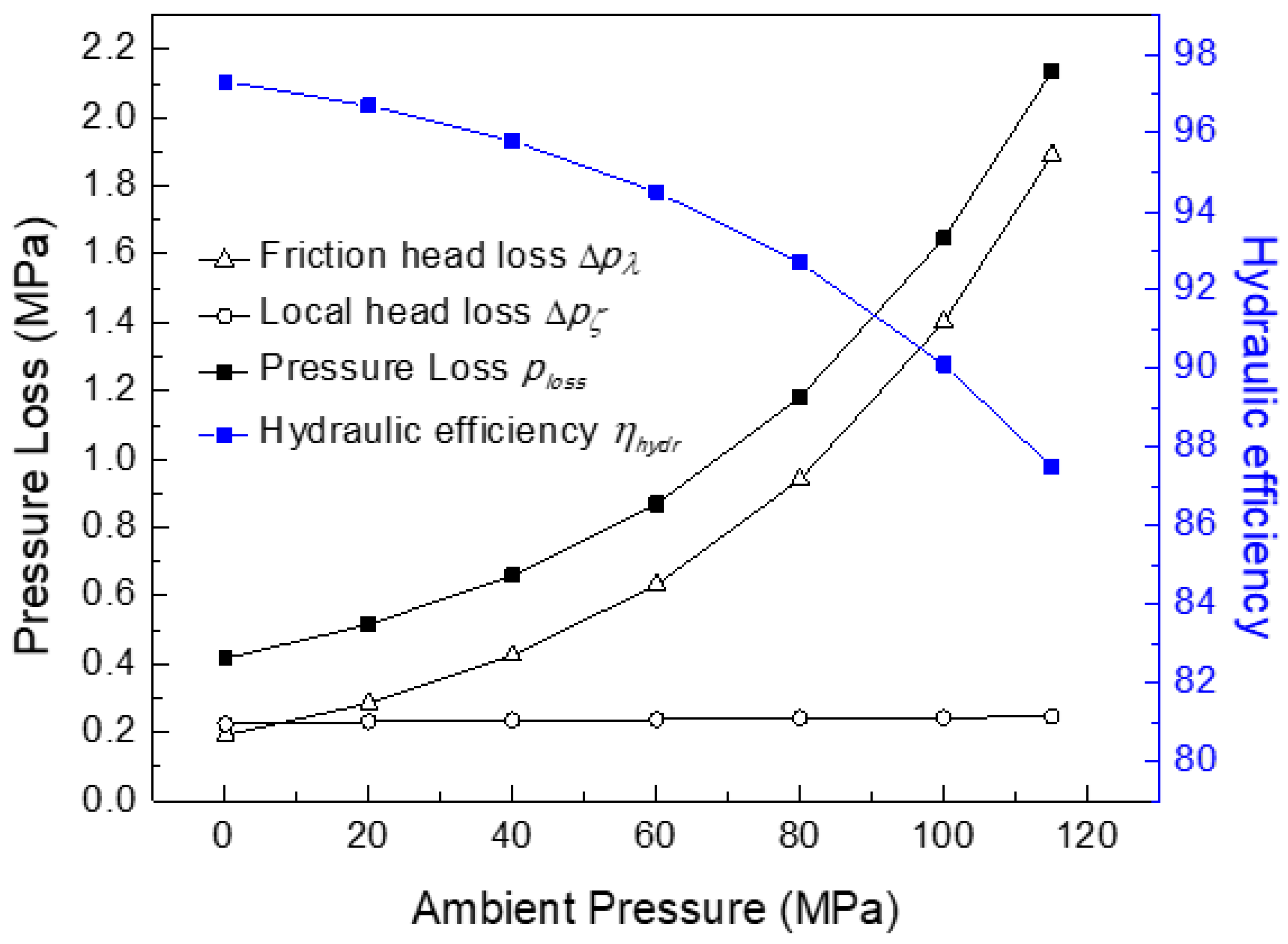
Equation (23) ignores internal leakage of the spool valve and cylinder piston, and emphasizes the effect of pressure loss on hydraulic circuit efficiency. Among them, the friction head loss $\Delta p_{\lambda }$ is caused by the viscous friction between the oil and the pipe wall, so it is mainly affected by the viscosity of the oil. The local (elbow) pressure loss $\Delta p_{\zeta }$ is caused by the formation of vortices at the elbow when the flow direction changes, which increases the resistance loss and is mainly affected by the oil density.

The variation of pressure loss is shown in Figure 23. As the oil viscosity increases, the friction head loss and local pressure loss increase, and the friction head loss changes more widely. When the water depth exceeds 6000 m, the pressure loss curve rises faster. The effect of pressure loss on the hydraulic circuit efficiency becomes non-negligible. Therefore, when designing the deep-sea hydraulic system, the layout should be reasonable, and the length of the pipeline should be shortened as much as possible.

3.4. System Efficiency

The Figure 24 shows the power transfer process between devices, and summarizes the variations of power loss during the transfer process. It can be seen from Figure 24 that the increase in oil viscosity directly leads to a decrease in the efficiency of deep-sea oil-filled motors and hydraulic circuits. The hydraulic-mechanical efficiency of the external gear pump is negatively affected by the increase of oil viscosity, while its volumetric efficiency increases with the increase of oil viscosity. The opposite trend of the two causes the gear pump efficiency to increase first and then decrease.

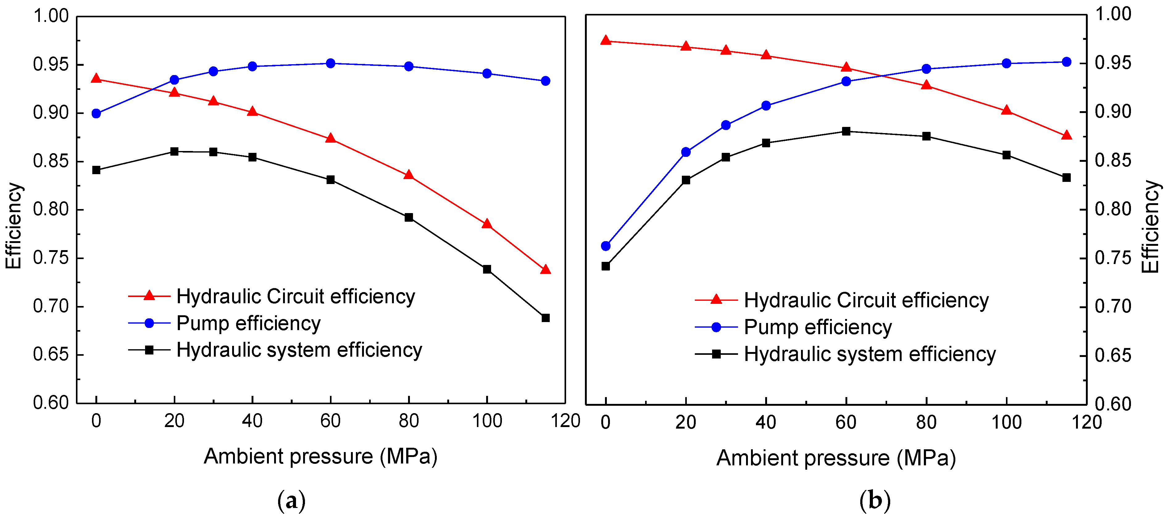
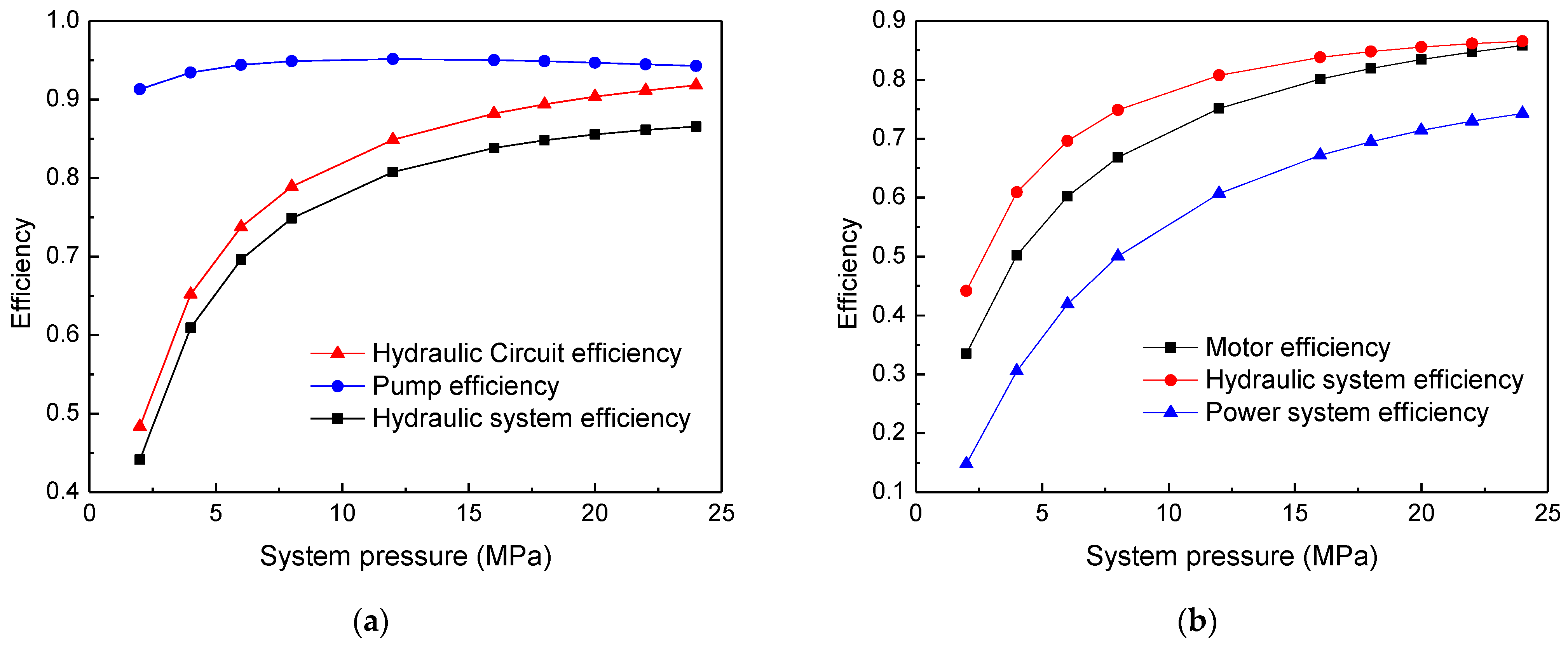
The efficiency characteristics of the motor, pump and hydraulic circuit are studied before, and the efficiency curve of the hydraulic system (pump + hydraulic circuit) and power system (motor + hydraulic system) of the deep-sea hydraulic source can be further obtained, as shown in Figure 25. In both working conditions, with the increase of ambient pressure, the efficiency of the hydraulic system and power system both increase first and then decrease. The oil viscosity increases exponentially with the increase of the pressure. After entering the pressure range of “Hadal zone” with the depth over 6000 m, the power loss and friction head loss caused by the viscous frictional resistance will have a greater impact on the hydraulic system’s efficiency.

At the same time, compared with the maximum efficiency value, the power system efficiency at ambient pressure of 115 MPa only decreased by 8.3% (under operating condition: load pressure is 15~19 MPa). It has been preliminarily proved that under ideal conditions, using hydraulic oil of ISO VG10 viscosity grade and properly increasing the temperature of the oil tank can improve the efficiency of the hydraulic system at a depth of 10,000 m.

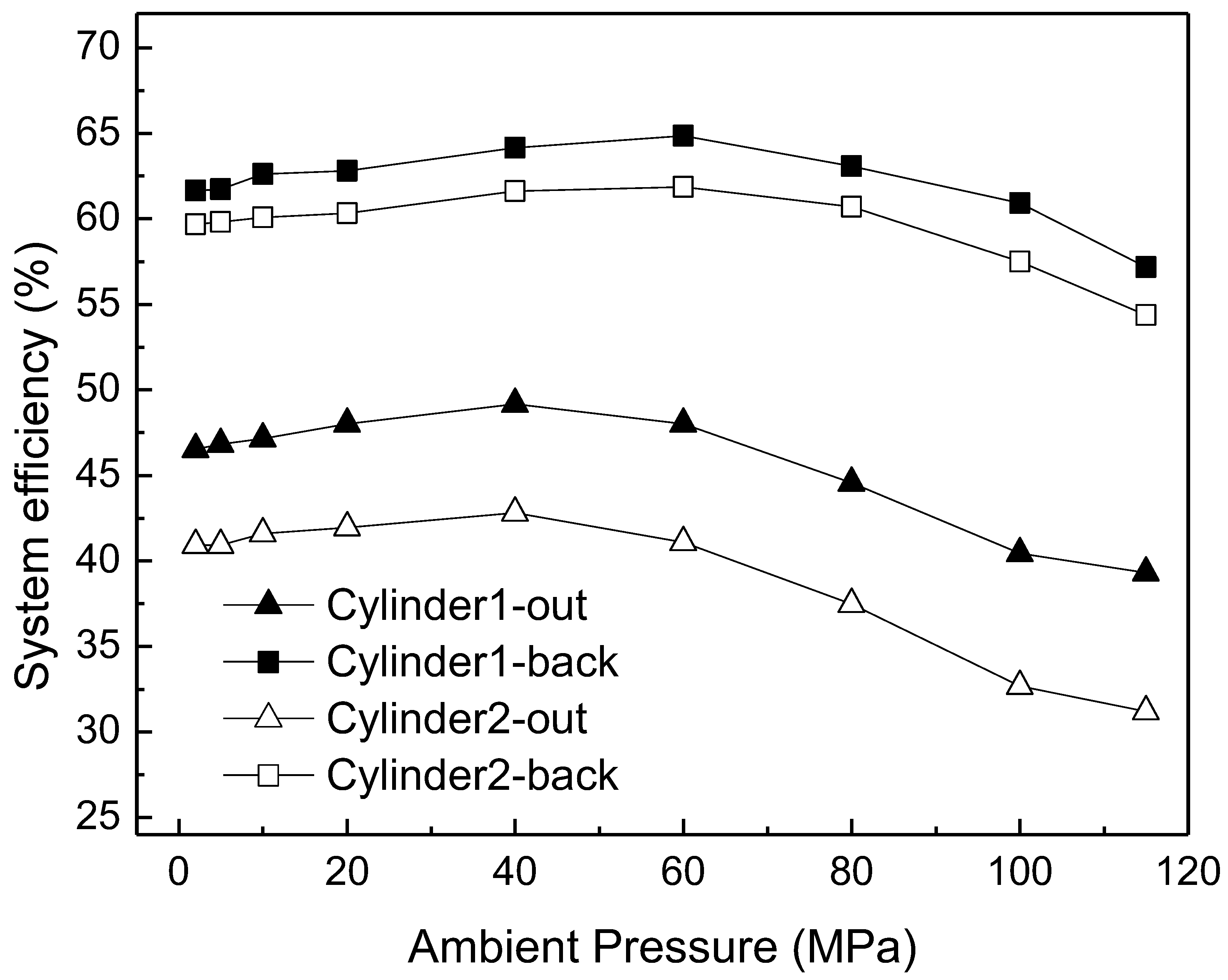
In order to directly reflect the variation of system efficiency under different load pressures, the system efficiency curves under different load pressures are calculated and drawn. During the calculation process, the motor speed and ambient pressure are unchanged. It can be seen from the Figure 26 that, with the same working parameters set, the system efficiency increases gradually with the increase of the load pressure. Therefore, in order to ensure higher system efficiency, the system should work as close as possible to the rated working pressure (21 MPa).

4. Experimental Setup and Result

4.1. Experimental Setup

The full-ocean-depth hydraulic source prototype was tested in two pressure cylinders from Zhejiang University and a research institute in China. The pressure cylinder from Zhejiang University is shown in Figure 27. They can reach the pressure levels of 60 MPa and 210 MPa respectively. The hydraulic source prototype studied in this paper has been tested in two pressure cylinders for two stages. This paper mainly analyzes the experimental data of the final test.

The prototype test system of the full-sea deep hydraulic source is shown in Figure 28. Various sensors and electronic control units are set up in the test system. During the experiment, data acquisition and signal transmission are required. Therefore, PLC is set up as the main control unit in the test system, and is connected with the motor driver and the data acquisition circuit.

The parameters of the pressure sensor used in the prototype are shown in

Table 10. Parameters of the pressure sensor.

Full Scale Sensitivity	Total Error Band	Operating Temperature	Pressure Range (Bar)	Proof Pressure (Bar)	Burst Pressure (Bar)
2.6 mV/V	±0.025%	−40 °C to +218 °C	0–1723	2068	2413

. The maximum ambient pressure in the pressure cylinder test reached 144 MPa, which is within the pressure resistance range of the sensor. Two pressure sensors are set in the system, which are respectively set at the pressure inlet of the solenoid directional valve and the center of the oil tank. The signal of the pressure sensor is amplified by the signal amplifier and input to the signal acquisition system.

Considering that commercially available flowmeters cannot withstand high external pressures, an alternative solution for measuring average flow was devised. An asymmetric hydraulic cylinder is connected to the load circuit, and two travel switches are arranged on the movement path of the extension rod. Considering the corrosion of seawater, the contacts of the selected travel switch are made of silver. By measuring the time difference between the signals, the average flow can be calculated. In order to verify the measurement accuracy of this method, a gear flowmeter is connected to the pressure inlet of the directional valve. The performance parameters are shown in

Table 11. Performance parameters of the gear flowmeter.

Accuracy Error	Linearity Error	Starting Point (L/min)	Measuring Range (L/min)
±0.3%	±0.1%	0.03	0.6–160

. The gear flowmeter calculates the flow rate by calculating the phase difference of the square wave signals of the two channels, and guarantees the linearity error and accuracy of the measurement result.

Under the conditions of cylinder rod extension and retraction, three sets of time differences were measured and averaged. Based on the flow value measured by the flow meter, the error of the calculated average flow rate can be obtained, as shown in Figure 29. It can be seen from the figure that the error of this flow measurement scheme does not exceed ±0.6%. Comparing the data in this figure, it can be seen that the error of the calculated flow is larger when the motor speed is low. This is mainly related to the dimensional error of the travel switch. In general, when the maximum output flow of the gear pump is 16 L/min, the calculated deviation value of the flow is less than 0.06 L/min.

4.2. Experimental Prceoss

The deep-sea hydraulic source prototype is placed at the bottom of the pressure cylinder, and the control systems such as motor drives are placed outside the pressure cylinder. The two are connected by an ultra-high pressure watertight cable. The sensor data from the hydraulic source prototype is transmitted through the watertight cable, and is input into the PLC through the filter circuit for display and storage. The control signals of the motor and the solenoid valve are transmitted from the PLC, and are input to the corresponding electrical components through the motor driver and the watertight cable.

The pressure variation curve of the pressure cylinder is shown in Figure 30. Eight pressure test points were selected in the pressure range of 0~115 MPa. The safe pressurization rate was set as 1 MPa/min in the pressure rise stage. When the test pressure is reached, the pressure cylinder enters the pressure-holding state. After completing the performance test under the ambient pressure of 115 MPa, turn off the motor power. Raise the ambient pressure to 144 MPa and hold the pressure for 30 min. Observe the sensor signal to verify the pressure capability of the system.

In the pressure holding stage of the pressure cylinder, the specific test steps are as follows:

(a) When the ambient pressure reaches the test points, the pressure cylinder enters the pressure holding stage, and turns on the motor power.

(b) After the motor runs stably, close the idler valve. Signal the solenoid directional valve to control the hydraulic cylinder, and complete a movement cycle of extension and retraction.

(c) Record the back pressure of the oil tank, the output pressure of the system, and the input power under different load conditions from the panel on the electrical control box.

(d) The signals of the position sensors are collected by the analog input module of the PLC. Record the calculated average flow from the PLC screen, and observe the displacement of the compensator piston in real time.

(e) Adjust the motor speed and repeat the above steps.

In order to ensure the scientificity of the measurement results, repeat the test process 2–3 times under different ambient pressures.

4.3. Result and Discussion

Figure 31 shows the temperature curve of the oil tank recorded in real-time during the pressure cylinder test. As can be seen from the figure, with the progress of the test, the temperature of the oil tank gradually increased, and then stabilized at around 32 °C. The temperature fluctuation did not exceed ±1 °C. The radiator is placed at the outlet of the relief valve, so the temperature fluctuation is mainly affected by the heating of the load throttle valve.

Comparing with the pressure variation curve of Figure 30, when the temperature of the oil tank rises from 26 °C to 31 °C, the ambient pressure is approximately 20 MPa. Therefore, when the ambient pressure is less than 20 MPa, the test data will be affected not only by the ambient pressure, but also by the temperature change of the oil. As the oil temperature increased to the stable level, the effect of the temperature difference on the test results gradually became weaker. The maximum temperature difference does not exceed 5 °C, so all data will be displayed. However, in order to ensure scientificity, the test data under the ambient pressure of 20 MPa to 115 MPa will be mainly used to verify the calculation results and support the conclusions.

During the holding pressure stage of 115 MPa, the system is always kept in an overflow state. The temperature variation curve in Figure 31 shows that, the heat dissipation efficiency of the selected radiator matches the thermal efficiency of the circuit. In general, during the pressure cylinder test, the temperature of the oil tank can be basically kept stable.

A manual throttle valve was used in the prototype test system. The opening of the throttle valve on each load circuit is fixed. The prototype test system is equipped with multiple load hydraulic cylinders. The effective working areas of the two chambers are different, so when the output flow remains unchanged, the movement speeds of the asymmetric hydraulic cylinders extending and retracting are different. Specifically, the damping coefficient is set as $B_P$, and the dynamic friction force of piston is $F_f$. Considering the stable state of the system, ignoring the inertial term and the nonlinear part of friction resistance, the load-pressure equations can be obtained.

When the hydraulic cylinder extends, $q_1\approx q_P$:

$$p_{P1}={\left(\frac{q_1}{C_d{A}_t}\right)}^2\frac{\rho }{2}+\frac{F_f{A}_1+B_P{q}_1}{A_1^2}$$

(24)

when the hydraulic cylinder retracts, $q_2\approx q_P$:

$$p_{P2}=p_2={\left(\frac{A_1}{A_2}\right)}^3{\left(\frac{q_2}{C_d{A}_T}\right)}^2\frac{\rho }{2}+\frac{F_f{A}_2+B_P{q}_2}{A_2^2}$$

(25)

As can be seen from the equation, the load pressure is greater when the hydraulic cylinder is retracted. Two loads with different throttle valve openings are selected. Among them, the throttle valve opening of the first load circuit (Cylinder1) is smaller, and the load pressure under the same working conditions is larger. The variation of load pressure and load flow with ambient pressure is shown in Figure 32 and Figure 33.

With the increase of ambient pressure and oil viscosity, the output flow under the four working conditions gradually increased. It can be seen from Figure 32 that the output pressure has not reached the opening pressure of the relief valve: 24 MPa. Therefore, the average load flow in Figure 33 can be approximately regarded as the output flow of the gear pump. That is, as the ambient pressure increases, the volumetric efficiency of the gear pump increases gradually. Different from the theoretical calculation, the flow through the throttle valve increases in the test, and the load pressure also increases gradually. The increase in pressure will reduce the volumetric efficiency. Thus, the output flow in Figure 33 is affected by both viscosity and load pressure. However, it can be seen from Figure 33 that within the working pressure range, the oil viscosity has a greater positive effect on the volumetric efficiency of the gear pump. Therefore, the flow curve in Figure 33 can still reflect the variation trend of the volumetric efficiency of the gear pump.

The voltage and current input to the motor can be read from the output port of the motor controller. The input power of the motor and the output power of the prototype can be calculated separately. Further, the total efficiency of the power system (motor + hydraulic system) can be obtained, as shown in Figure 34. It can be seen from the figure that the variation trend of the system efficiency is basically consistent with the calculation results in Figure 25. As the environmental pressure increases, the system efficiency first increases and then decreases. It can be seen from Figure 34 that under the operating conditions of the actuator (load pressure is 15~19 MPa), the efficiency of the power system at an ambient pressure of 115 MPa is reduced by 11.8% compared to the maximum efficiency.

Different from the calculation result in Figure 25, the load pressure in Figure 32 is not constant at 6 MPa and 15 MPa. For a throttle valve with a constant opening, the load pressure will continue to increase as the ambient pressure increases. It can be seen from Figure 32 that under the two working conditions of “cylinder-out”, the amplitude of the load pressure rise is relatively low, and is basically stable at around 4 MPa and 6 MPa. However, in the two working conditions of “cylinder-back”, the change of load pressure is more obvious. Figure 26 shows that under the same ambient pressure, the higher the load pressure, the higher the system efficiency. Therefore, compared with the test curve in Figure 34, when the load pressure is constant, the decreasing trend of the system efficiency curve will be more obvious. Under the same ambient pressure, the value of the system efficiency will also be lower. That is, the power loss caused by viscous friction has a more obvious effect on system efficiency.

In order to measure the oil friction loss of the deep-sea oil-filled motor under different ambient pressures, the idling power of the motor without oil filling was measured under the atmospheric pressure. In order to ensure the consistency of the load condition, the no-load condition means that the idling valve in the hydraulic circuit is opened, and the oil flows directly back to the oil tank without passing through the actuator. According to Equation (5), the input power of the motor is divided into four parts: copper loss, iron loss, friction loss and output power. Therefore, ignoring the wind friction loss, the idling power in the atmospheric environment mainly includes copper loss, iron loss, bearing friction loss and output power. By measuring the idling power of the oil-filled motor under different ambient pressures, the oil friction loss of the rotor under different ambient pressures can be obtained, as shown in Figure 35.

It can be seen from Figure 35 that the variation trend of the measured oil friction loss is consistent with the fluid simulation results, but the measured value is larger. Analyze the reasons for the deviation:

(1) The inner surface of the stator is relatively rough after encapsulation, while the surfaces of the stator and rotor in the simulation model are smooth. In the simulation model, the groove between the permanent magnets and the flow field at the end face are simplified in structure. These factors will increase the oil friction loss.

(2) As the viscosity of the oil increases, the viscous friction loss of the gear pump and hydraulic circuit increases. Under the same working conditions, the output power of the motor will also increase. At the same time, as the armature current increases, the copper loss and iron loss will also increase.

(3) The oil temperature set in fluid simulation is 26 °C. In the pressure cylinder test, when the motor is just started, the oil temperature is consistent with the ambient water temperature (city water supply in winter: 16 °C), and the temperature changes continuously with the running time.

Assuming that the uncertainty caused by temperature on the measurement results is not considered, it can be obtained that the oil friction loss calculated in Figure 35 is larger than the actual value, but the variation trends are consistent.

5. Conclusions

This paper mainly studies the efficiency characteristics of the deep-sea hydraulic source system in the full-sea deep pressure range. Firstly, the effect of ambient pressure on the efficiency characteristics of the motor, pump and hydraulic circuit is analyzed. Moreover, the pressure cylinder was used to simulate the high pressure in the deep sea, and the efficiency characteristic of the hydraulic source prototype was tested. Based on the temperature-viscosity data in the reference, the pressure-viscosity curves of Mobil Nuto H10 hydraulic oil at 25 °C and VELOCITE No. 5 hydraulic oil at 80 °C were fitted, respectively. The deviation of the two fitted curves does not exceed ±0.15%.

When studying the efficiency characteristics of deep-sea oil-filled motors, the variation of oil friction loss with environmental pressure is mainly studied. The theoretical calculation and simulation analysis of the simplified model and the actual model with grooves are carried out respectively. The results show that the oil friction loss of the motor rotor increases gradually with the increase of the ambient pressure. The grooves on the rotor surface disturb the flow field in the gap and significantly increase the oil friction loss.

When studying the efficiency characteristics of the gear pump, the volumetric efficiency and hydraulic-mechanical efficiency as a function of the oil viscosity were mainly studied. Bring in the gear pump’s structure data and plot the ambient pressure-efficiency curve. The results show that the volumetric efficiency and the hydraulic-mechanical efficiency have opposite trends. When the oil viscosity is in the lower range, the volumetric efficiency increases more greatly with the increase of viscosity. Therefore, as the ambient pressure increases, the overall efficiency of the pump first increases and then decreases.

For hydraulic circuits with fixed throttle loads, the effects of friction head loss and local pressure loss on efficiency are mainly studied. The results show that with the increase of ambient pressure, the pressure loss in the pipeline increases continuously. Moreiver, in the deep sea environment with the depth over 6000 m, the influence of pressure loss on the efficiency of the hydraulic circuit increases significantly.

Under ideal conditions, the efficiency characteristic curves of the hydraulic system and power system are calculated and plotted. In the pressure cylinder, the experimental study and data measurement of the hydraulic source prototype were carried out. After processing the test data, the system’s output characteristic curve and the variation curve of the motor’s oil friction loss are obtained. The experimental results are consistent with the theoretical calculation results. When the load is a fixed throttle valve and the motor speed is constant, the system efficiency of the hydraulic source prototype first increases and then decreases with the increase of the ambient pressure. Moreover, the power system efficiency at ambient pressure of 115 MPa is reduced by 11.8% compared to the maximum value.

In summary, when the ambient pressure rises to 100 MPa, the oil viscosity will increase significantly. Therefore, the Nuto H10 hydraulic oil with the lower viscosity was used in the prototype. When the ambient pressure is lower, the system efficiency is more affected by the volumetric efficiency of the gear pump. As the ambient pressure increases, the influence of viscous friction loss on the system efficiency increases continuously, which directly leads to a gradual decrease in the system efficiency.