A Fault Diagnosis Method for the Autonomous Underwater Vehicle via Meta-Self-Attention Multi-Scale CNN

Abstract

Autonomous underwater vehicles (AUVs) are an important equipment for ocean investigation. Actuator fault diagnosis is essential to ensure the sailing safety of AUVs. However, the lack of failure data for training due to unknown ocean environments and unpredictable failure occurrences is challenging for fault diagnosis. In this paper, a meta-self-attention multi-scale convolution neural network (MSAMS–CNN) is proposed for the actuator fault diagnosis of AUVs. Specifically, a two-dimensional spectrogram of the vibration signals obtained by a vibration sensor is used as the neural network’s inputs. The diagnostic model is fitted by executing a subtask-based gradient optimization procedure to generate more general degradation knowledge. A self-attentive multi-scale feature extraction approach is used to utilize both global and local features for learning important parameters autonomously. In addition, a meta-learning method is utilized to train the diagnostic model without a large amount of labeled data, which enhances the generalization ability and allows for cross-task training. Experimental studies with real AUV data collected by vibration sensors are conducted to validate the effectiveness of the MSAMS–CNN. The results show that the proposed method can diagnose the rudder and thruster faults of AUVs in the cases of few-shot diagnosis.

1. Introduction

The oceans contain a great number of natural resources and play a vital role in human development, but  ocean exploration remains challenging. As an efficient way of apprehending ocean exploration and utilization, AUVs have gained wide application in marine ecological research, mineral resource exploitation, scientific exploration, and the military. However, the complex marine environment poses significant challenges to AUV operations. The unknown ocean conditions may cause equipment malfunction, leading to mission failure or even equipment loss. Therefore, for the purpose of ensuring sailing safety, it is important to identify the failures and diagnose the actuator faults of the AUVs.

In recent years, various researchers have conducted a significant number of studies in the field of actuator fault diagnosis of AUVs. The health status of the actuator is diagnosed and identified by machine learning and deep learning methods. Fuzzy logic torque controllers with nonlinear friction compensation are used to improve the deterioration of trajectory tracking performance in rotating tandem elastic actuator systems caused by these nonlinear elements and to optimize trajectory tracking performance [1]. To diagnose thruster faults in AUVs under noisy environments, Sun et al. [2] proposed a thruster fault diagnosis method for AUVs based on deep neural networks and denoising autoencoder. Liu et al. [3] proposed a deep reinforcement learning-based controller in a simulation environment for studying the control performance of the vector thruster. The information that can be measured by the sensors inside the AUVs is used as an input parameter. Tsai et al. [4] proposed a fault diagnosis method for underwater thrusters based on deep convolutional neural networks, where the raw data were transformed from the time domain to the frequency domain by fast Fourier transform and used as the input to the neural network. Chu et al. [5] proposed an underwater thruster fault diagnosis method based on the random forest regression and support vector machine, which mainly solves the problem of insufficient diagnostic accuracy due to sample imbalance. Zhu et al. [6] proposed a fault diagnosis method based on Bayesian networks to solve the problem of difficulty in locating specific faults in the thrusters of autonomous underwater vehicles. A deep belief network is introduced in the multi-sensor information fusion model to identify uncertain and unknown signal, continuously changing the failure modes of deep-sea manned submersible thrusters [7]. The FDI method proposed by Talebi et al. [8] is used to detect, isolate, and identify the severity of actuator failures in the presence of disturbances and fault uncertainty in the model. To improve the performances of thruster fault diagnosis, Tian et al. [9] proposed a possible fuzzy C-means algorithm for thruster fault classification. Omerdic et al. [10] proposed a novel thruster fault diagnosis and adaptation system for open-frame underwater vehicles. The FDS monitors the status of each thruster using a fault detection unit associated with each thruster, which is capable of detecting the internal and external fault states of the thruster. Raanan et al. [11] proposed a Gaussian particle filtering algorithm to estimate the failure model of AUVs. The Bayesian algorithm is used to implement the fault detection of AUV thrusters, and a nearest neighbor classifier is used to accomplish the fault diagnosis. Ji et al. [12] proposed a new sequential convolutional neural network (SeqCNN), where a model-free fault diagnosis method is based on deep learning algorithms. The proposed SeqCNN aims to extract global and local features from state data and classify the extracted information into different fault types. Yeo et al. [13] proposed a system that can monitor the health of AUV thrusters using a convolutional neural network (CNN). The acoustic signal of the thruster was used as input data to achieve the fault diagnosis of the thruster of the AUVs. Tsai et al. [14] proposed a modified CNN based on merging two signals to classify faults. Experimental results show that the proposed multi-signal approach achieves excellent thruster fault diagnosis results. Kim et al. [15] proposed a fault detection system in which new vibration data were generated using a generative adversarial network (GAN) and was applied to a long short-term memory neural network. In the fault detection experiments of the underwater thruster, the vibration characteristics of the vibration sensor data obtained from the experiments and the data generated by the GAN were compared and analyzed using the fast Fourier transform. To study the model-free trajectory tracking control problem of AUVs, Bingul et al. proposed a novel control structure based on the model-free control principle to ensure stable and accurate trajectory tracking of AUVs in complex underwater environments [16].

The rudder is a kind of servo mechanism which is widely used in the control system of aircraft, ships, missiles, navigators, etc. It receives control signals and drives the deflection of the rudder plate to control the navigator’s attitude and trajectory. It is necessary to analyze the state, static, and dynamic parameters of the rudder system during operation to ensure the accurate control of the rudder system. Wang et al. [17] proposed a convolutional neural network combining a particle swarm optimization algorithm and a grayscale optimization algorithm to accomplish the automatic multi-fault classification of rudders. An adaptive sampling algorithm (ASCIN) considering information instances was proposed by Li et al. [18,19] The optimal parameters of ASCIN were searched by the whale optimization algorithm to overcome the limitations of conventional detection devices. Zhou et al. [20] proposed a deep neural network-based health monitoring method. Autoencoders were used to reduce the feature dimensionality and combined with the SoftMax classifier for health monitoring. Ren et al. [21] proposed a fault diagnosis method based on a Back Propagation Neural Network (BPNN), which was optimized using the SODEBBO optimization algorithm to accomplish the automatic classification of multiple faults in rudder testing. Qin et al. [22] optimized the BPNN with particle swarm optimization hybrid fruit fly algorithm to improve the diagnostic performance. Chang et al. [23] proposed a random forest algorithm based on a shuffle frog-jumping algorithm to make the decision-making of the model more efficient and accurate. Xu et al. [24] proposed the combination of a nonlinear unknown input observer with adaptive thresholding, which helps to reduce the effect of model uncertainty. Chang et al. [25] proposed a machine learning method-based optimized decision tree algorithm to solve the common decision difficulties caused by low-precision decisions and high voting competition in tree models. Jiang et al. [26] used finite impulse response and principal component analysis to solve the fault diagnosis problem of AUV actuators under winding failure and improve the overall reliability of underwater vehicles. Xuan et al. [27] proposed a fault diagnosis method based on convolutional neural networks and autoencoders to solve the problem of fault detection and isolation in uncoupled fault modes. Jia et al. [28] proposed an ensemble deep autoencoder based on an extreme learning machine, which has significant advantages in handling imbalanced data.

However, in previous studies, machine learning and data augmentation methods have been widely used for fault analysis and diagnosis. Traditional machine learning, which heavily relies on a priori knowledge, often struggles with selecting appropriate features and can result in poor performance. Data augmentation methods, on the other hand, primarily generate more similar samples to expand the dataset, and while GAN can also perform data augmentation, they inherently require a large amount of data to accurately learn the data distribution of the samples. In practical underwater equipment working environments, the equipment is often expensive, and simulating failures can incur substantial costs, leading to sparse data. Consequently, data augmentation methods also suffer from certain drawbacks.

A fault diagnostic method based on meta-deep learning is thus proposed in this paper to achieve fault identification in the cases of a few-shot diagnosis. Specifically, the mechanical equipment’s vibration signals are first collected to create a two-dimensional spectrogram with time–frequency information. Next, a feature extraction model and classifier are built. This model is optimized using a subtask-based gradient descent optimization approach, in order to extract degraded information that can represent the fault status. Then, a multi-scale self-attentive convolutional neural network is proposed for feature extraction, which allows for the model to locate critical features and obtain various degradation indicators considering both global and local information. The contributions of this work are summarized as follows:

• A diagnostic model that considers both global and local information in feature extraction is developed by introducing the multi-scale deep learning method into the self-attentive mechanism. The extracted features that are more suitable for characterizing the health status of the AUV actuators can be automatically obtained for fault diagnosis and classification.
• The meta-learning approach is incorporated so that the diagnostic model can be trained iteratively with few-shot and converge rapidly. The meta-learning approach enables cross-task training and completes cross-device fault diagnostics by enhancing the generalization abilities without requiring a large amount of labeled data.
• A meta-self-attentive multi-scale deep learning method for actuator fault diagnosis of AUVs is proposed to diagnose the rudder and thruster faults with a few-shot. Experimental studies demonstrate the effectiveness of the proposed method in actuator fault diagnosis of AUVs.

The background information in Section 2 serves as the foundation for the remainder of this essay. Our suggested few-shot identification method is thoroughly explained in Section 3. The AUVs dataset is demonstrated in Section 4 along with a thorough experimental validation that contrasts it with other diagnosis techniques. A summary of this paper and a prognosis for further investigation are provided in Section 5.

2. Background

This section consists of three subsections that introduce the fundamental concepts required to build the model. The first subsection explains the concept of small sample learning and the objective function for model optimization. The second subsection covers the method of meta-learning and the dataset division. Lastly, the third subsection discusses the self-attentive mechanism concept and how to apply it.

2.1. Few-Shot Learning

Few-shot learning attempts to overcome the problem of insufficient data, whereas traditional machine learning and deep learning call for a high number of training samples and will significantly worsen recognition performance in the event of insufficient training samples. Nonetheless, in this instance, few-shot learning also produces good recognition performance. From a learning task $\mathcal{T}$ [27], a small-scale training set $D_{\mathrm{train}}={\left\{(x_i,y_i)\right\}}_{n=1}^N$, and a test set $D_{\mathrm{test}}={\left\{x_i\right\}}_{m=1}^M$, define $P(x,y)$ is the joint probability distribution of x and y, $\stackrel{⌢}{h}$ is the optimal hypothesis from x to y, while less-sample learning can obtained $\stackrel{⌢}{h}$ by learning on $D_{train}$ and testing on $D_{test}$. To approximate $\stackrel{⌢}{h}$, it determines a hypothetical space H consisting of a hypothesis $h(·;\theta )$, which $\theta$ represents all the parameters used by h. It can be thought of as an optimization process that finds H to obtain $\theta$, holding the optimal $h^{*}\in H$ in the training set.

The objective function, which is written as Equation (1), is the function that is typically maximized or minimized to determine the corresponding parameter weights in traditional machine learning and deep learning problems. Equation (2) gives a concrete representation of the loss function.

$$\underset{\theta }{min}{\sum }_{(x_i,y_i)\in D_{train}}Loss(h(x_i;\theta ),y_i)$$

(1)

$$Loss(h(x_i;\theta ),y_i)=-{\sum }_{x^{\left(j\right)},y^{\left(j\right)}\in D}{f}_{\theta }\left(x^{\left(j\right)}\right)log\left(y^{\left(j\right)}\right)$$

(2)

where $\theta$ is defined as the parameter of the less-shot learning model.

The sample size N is much smaller in few-shot learning, leading to more pronounced deviations between target values. The resulting model $h_N$ is likely to be overfitted, so it is crucial to investigate appropriate methods for few-sample learning.

2.2. Meta-Learning

A large amount of data from a certain scenario is generally utilized to train a model in machine learning, and the model needs to be retrained when the scenario changes. However, this is not in line with the law of human learning knowledge, as humans and even infants have the inherent ability to rapidly learn new concepts with a small number of samples and accurately summarize them in unknown situations.

The intelligent recognition models currently established require large-scale data, but the cost of obtaining these data is generally relatively high, resulting in unsatisfactory recognition results. These basic recognition models are all focused on a specific task, and when encountering cross-task situations, they need to acquire a large amount of data in another task domain to retrain the network. This is in stark contrast to humans mastering knowledge and migrating to uncharted territory. However, meta-learning [29] makes it possible to discover prototypes in a given domain under specific tasks and optimize the network by extracting general knowledge of different subtasks. The method can be seen as a solution for few-shot learning, mining more valuable parameters and enhancing its generalization ability among other differently distributed data [27].

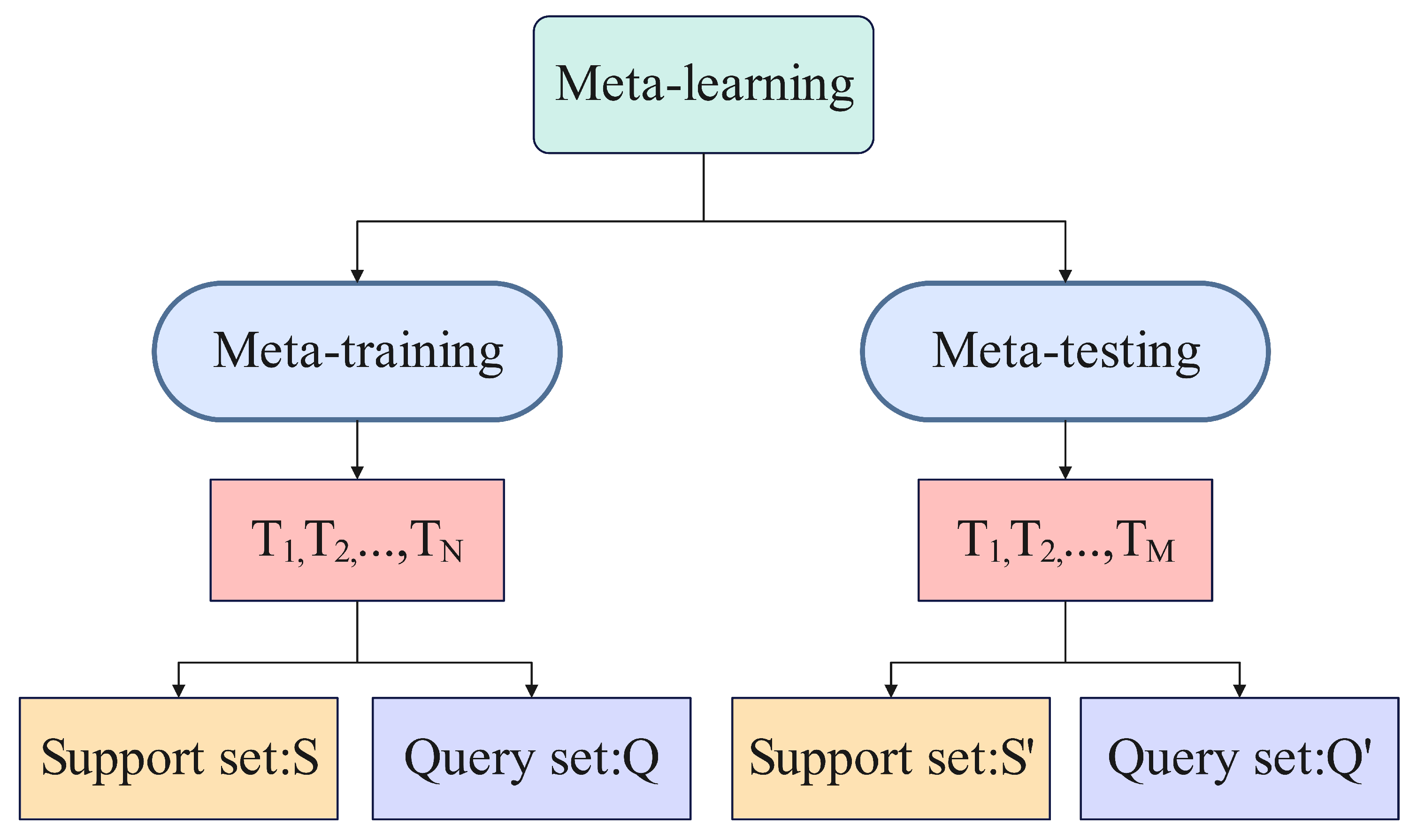
The training unit is the task in meta-learning, which is generally divided into a training task and a testing task. Many subtasks need to be prepared to learn the model, aiming to learn better hyperparameters that are required to fit the new tasks. A learning task $T=\{y,f\}$ consists of two parts: the label space y and the prediction function f. The prediction function is trained on a given feature vector and label pair $\{x_i,y_i\},x_i\in x,y_i\in y$.

2.3. Self-Attentive Mechanism

Attention is a complex cognitive function that is indispensable to humans, which refers to the ability to choose some information while ignoring another. The ability of the human brain to select, consciously or unconsciously, small portions of useful information to focus on from this large amount of input and to ignore other information is known as attention. When using neural networks to process a large amount of input information, you can also learn from the attention mechanism of the human brain and select only some key information inputs for processing to improve the efficiency of neural networks. It is also possible to improve the efficiency of the neural network by drawing on the attention mechanism of the human brain when a neural network is used to process a large amount of input information.

Let us use $X=[x_1,x_2,\cdots ,x_N]\in {\mathbb{R}}^{D\times N}$ to represent N groups of input information, where the D dimensional vector $x_n\in {\mathbb{R}}^D$, $n\in [1,N]$ represents a set of input information. To save computing resources and reduce the amount of calculation, it is not necessary to input all the information into the neural network, but only to select some task-related information from X. The calculation of the attention mechanism can be divided into two steps: one is to calculate the attention distribution on all input information, and the other is to calculate the weighted average of the input information according to the attention distribution. To select task-related information from input vector $[x_1,x_2,\cdots ,x_N]$, a task-related representation called query vector needs to be introduced, and the correlation between each input vector and query vector is calculated through a scoring function.

In order to improve the feature extraction ability of the model, the self-attentive mechanism often adopts the Query-Key-Value (Query-KV) model. Given the query vector $q_n\in Q$, the output vector $h_n$ can be obtained by Equation (4).

$${\alpha }_{n,j}=softmax\left(s(k_j,q_n)\right)$$

(3)

$$h_n=att((K,V),q_n)=\sum _{j=1}^N{\alpha }_{nj}{v}_j$$

(4)

where $n,j\in [1,N]$ is the position of the sequence of output and input vectors, ${\alpha }_{nj}$ denotes the weight of the first output concern to the first input, $s(\cdot )$ denotes the scoring function, $k_j$ denotes the jth element of the value vector, and $v_j$ denotes the jth element of the value vector.

Generally, the scoring function is calculated using the method of scaling the dot product, with the formula is $s(h,q)=\frac{h^{T}q}{\sqrt{D}}$, and the output sequence can be calculated as

$$H=softmax\left(\frac{K^{T}Q}{\sqrt{D_k}}\right)V$$

(5)

where $K,V,Q$ are the key, value, and query matrix, respectively. $\sqrt{D_k}$ is a normalization constant to ensure gradient stability.

3. Proposed Method

This section consists of three subsections that introduce the proposed method and the steps involved in building the network model. The first subsection describes the overall framework and implementation steps for the fault diagnosis of AUV actuators. The second subsection explains the self-attentive multiscale feature extraction method. Lastly, the third subsection explains the meta-learning optimization method in the case of a few-shot.

3.1. Research Steps of Intelligent Fault Diagnosis

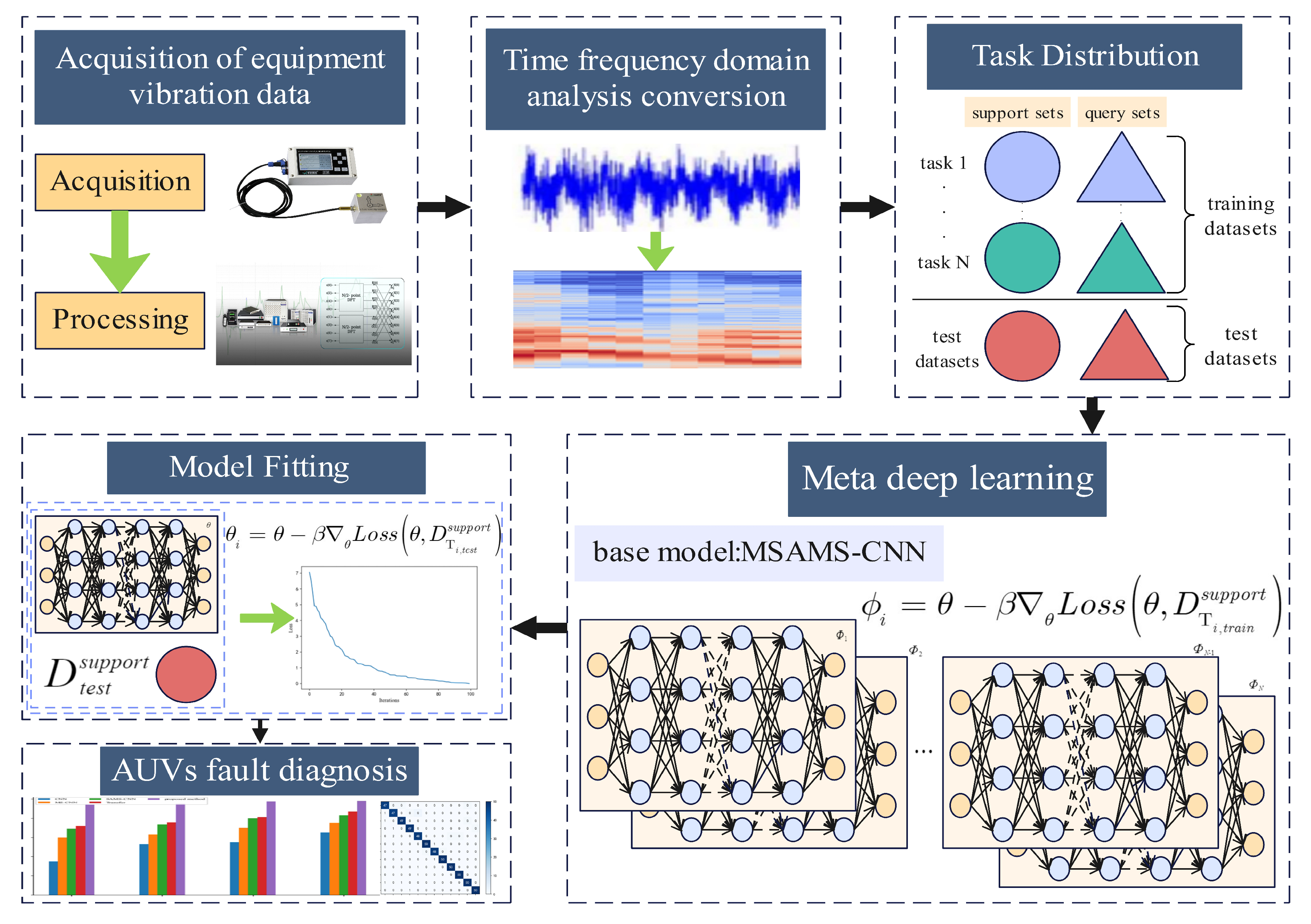
This section proposes a fault diagnosis method based on meta-learning, which is mainly applied to few-shot learning. Figure 1 represents the overall framework of few-shot fault diagnosis consisting of six main steps.

First, the vibration data of the equipment movement are collected as the original signal. The signal is normalized to avoid the presence of singular values that affect the convergence speed of the network.

Then, the short-time Fourier transform is performed on the processed data to obtain a two-dimensional feature map that contains time-domain information and frequency-domain information, which is convenient for the subsequent feature extraction.

Third, in contrast to the traditional deep learning fitting model, the training and testing datasets are redefined to perform model fitting in a subtask-based learning approach. The task-based training approach is to divide the data into two parts: the training task and the testing task. The training dataset is usually a dataset from other related domains, which is used to assist learning. In this part of the data, the support set serves as the learning data for each subtask, while the query set is used for cross-subtask training to learn the meta-knowledge of the model, aiming to obtain more sensitive parameter states of the established meta-multi-scale feature extraction model. The division between the support set and the query set is different in the test dataset. The former is to fine-tune the meta-learning framework that is already fitted by the training task dataset, while the latter is to complete a small number of predictions and verify the feasibility of the established model.

Fourth, a meta-learning model based on self-attentive multi-scale feature extraction is proposed for the fault diagnosis problem of AUVs based on the industrial status of sparse fault data, which can be used to achieve fault identification and health prediction for AUVs.

Fifth, the model is trained and fine-tuned using the data segment in the third step and working on finding the optimal parameters.

Finally, the already fitted meta-learning network is used for fault diagnosis of the autonomous underwater vehicle.

3.2. Fault Diagnosis Model with Self-Attentive Multi-Scale Feature Extraction

In recent years, CNNs have been widely used in the field of fault detection of mechanical equipment, which usually consists of convolutional layers, batch normalization layers, and pooling layers, and has significant capabilities in extracting features. Although CNNs can be found to perform well in this field, in some studies [30,31], the performance of this method needs to be improved in the case of few-shot learning. This section will comprehensively use the knowledge of multi-scale kernel and self-attention mechanism to propose a self-attention multi-scale feature extraction model for the fault diagnosis of AUVs with a few-shot.

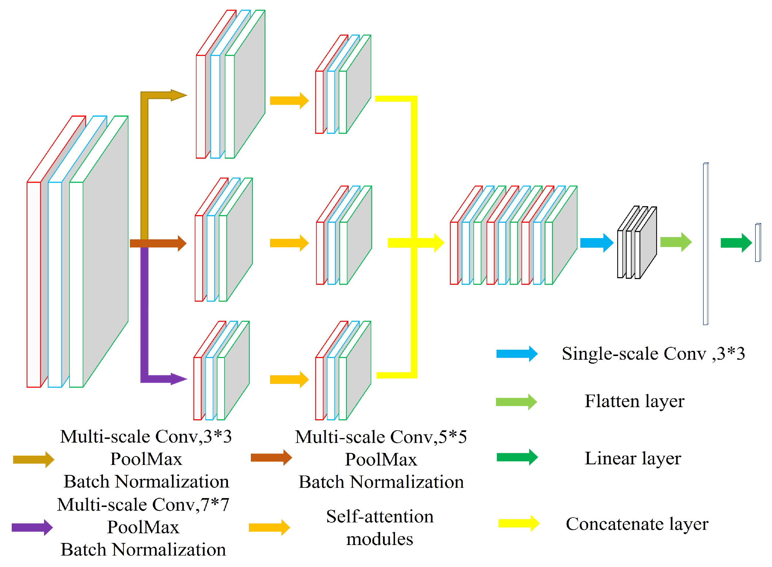
The proposed model contains three branches, i.e., three different convolution kernel sizes. Different convolution kernels are performed on the input data to obtain different types of features, and self-attention modules are added after the features are extracted by each convolution kernel. Multi-scale can take into account both global and local features, and the attention mechanism enables the model to learn important information autonomously and reduce the number of operations. To connect these three branches, a concatenate layer is used directly to connect the three branches. However, the output dimensions of different convolutional kernels are inconsistent, and pooling and batch normalization layers need to be added before the concatenation layer to ensure dimensionality consistency. Overall, the general architecture of the proposed model is shown in Figure 2, and the detailed steps are as follows:

The original data are first subjected to a short-time Fourier transform. The basic idea is to first multiply a function and a window function, then perform a one-dimensional Fourier transform, and obtain a series of spectral information by sliding the window function. These results are successively stitched together to obtain a two-dimensional time–frequency map. The basic operation formula is as follows:

$$X(t,\omega )={\int }_{-\infty }^{+\infty }x\left(t\right)h(t-\omega )e^{-j\omega t}dt$$

(6)

where $x\left(t\right)$ is the time domain signal, $h(t-\omega )$ is the window function, and X is used to represent the result of the short-time Fourier transform.

Input the spectrogram X to the multi-scale convolutional layer for feature extraction, and the convolution calculation formula is as follows:

$$Z_1(u,v)=\sum _{i=-\infty }^{\infty }\sum _{j=-\infty }^{\infty }{x}_{i,j}·k_{(u-i,v-j)}^1$$

(7)

$$Z_2(u,v)=\sum _{i=-\infty }^{\infty }\sum _{j=-\infty }^{\infty }{x}_{i,j}·k_{(u-i,v-j)}^2$$

(8)

$$Z_3(u,v)=\sum _{i=-\infty }^{\infty }\sum _{j=-\infty }^{\infty }{x}_{i,j}·k_{(u-i,v-j)}^3$$

(9)

among them, $k^1,k^2,k^3$ represent three different convolution kernels, and $Z_1,Z_2,Z_3$ represent the results calculated by different convolution kernels.

The results of the multi-scale convolution are down-sampled and normalized. The features are activated in the batch normalization layer using the ReLU activation function. The specific calculation formula is as follows:

$$({\stackrel{⌢}{Z}}_1,{\stackrel{⌢}{Z}}_2,{\stackrel{⌢}{Z}}_3)=maxpool(Z_1,Z_2,Z_3)$$

(10)

$$(A_1,A_2,A_3)=ReLU({\stackrel{⌢}{Z}}_1,{\stackrel{⌢}{Z}}_2,{\stackrel{⌢}{Z}}_3)$$

(11)

where ${\stackrel{⌢}{Z}}_1,{\stackrel{⌢}{Z}}_2,{\stackrel{⌢}{Z}}_3$ denote the result of the pooling operation and $A_1,A_2,A_3$ denote the output after normalization, which is dimensionally consistent throughout the processing.

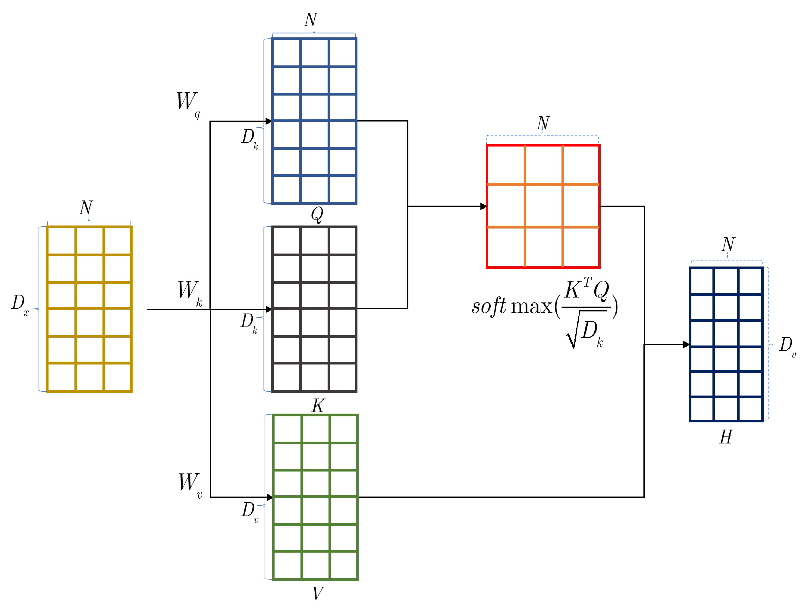
To further extract features, the model is equipped with the ability to extract important features autonomously through the self-attentive module, using $A_1,A_2,A_3$ features as input. Then, the input sequence is $A=[a_1,a_2,\cdots ,a_N]\in {\mathbb{R}}^{D\times N}$ and the output sequence is $H=[h_1,h_2,\cdots ,h_N]\in {\mathbb{R}}^{D_v\times N}$. The specific calculation process is as follows:

Each input $a_i$ is mapped to three different spaces. Figure 3 represents the transformation process to obtain the query vector $q_i\in {\mathbb{R}}^{D_k}$, the key vector $k_i\in {\mathbb{R}}^{D_k}$, and the value vector $v_i\in {\mathbb{R}}^{D_v}$. For the whole input sequence A, the linear mapping process can be abbreviated as Equations (12)–(14):

$$Q=W_{k}A\in {\mathbb{R}}^{D_k\times N}$$

(12)

$$K=W_{k}A\in {\mathbb{R}}^{D_k\times N}$$

(13)

$$V=W_{v}A\in {\mathbb{R}}^{D_v\times N}$$

(14)

where $W_q\in {\mathbb{R}}^{D_k\times D_x}$, $W_k\in {\mathbb{R}}^{D_k\times D_x}$, $W_v\in {\mathbb{R}}^{D_v\times D_x}$ are the parameter matrices of the linear transformation, $Q=[q_1,q_2,\cdots ,q_N]$, $K=[k_1,k_2,\cdots ,k_N]$, $V=[v_1,v_2,\cdots ,v_N]$ denote the matrices composed of query vector, key vector, and value vector, respectively.

For the query vector $q_n\in Q$, the output vector $h_n$ can be obtained by using the key-value pair attention mechanism of Equation (4).

Attention $H_1,H_2,H_3$ can be obtained by Equations (3)–(5) and (11)–(13).

Use a concatenate layer to merge the features of the three branches and turn the channel into a single-channel feature through point convolution, as follows:

$$H=concat(H_1,H_2,H_3)$$

(15)

The output features are further fed into the Softmax classifier for state identification and fault classification after the above operations. For clarity, the detailed parameters of the convolution part are given in

Table 1. Parameters of the convolution part.

Convolution Category		Convolution Kernel (Channel × Width × Height)	Strides
Multi-scale Conv	Conv1	(3,3,3)	(1,1)
	Conv2	(3,5,5)	(1,1)
	Conv3	(3,7,7)	(1,1)
Signal-scale Conv	Conv4	(3,3,3)	(1,1)

.

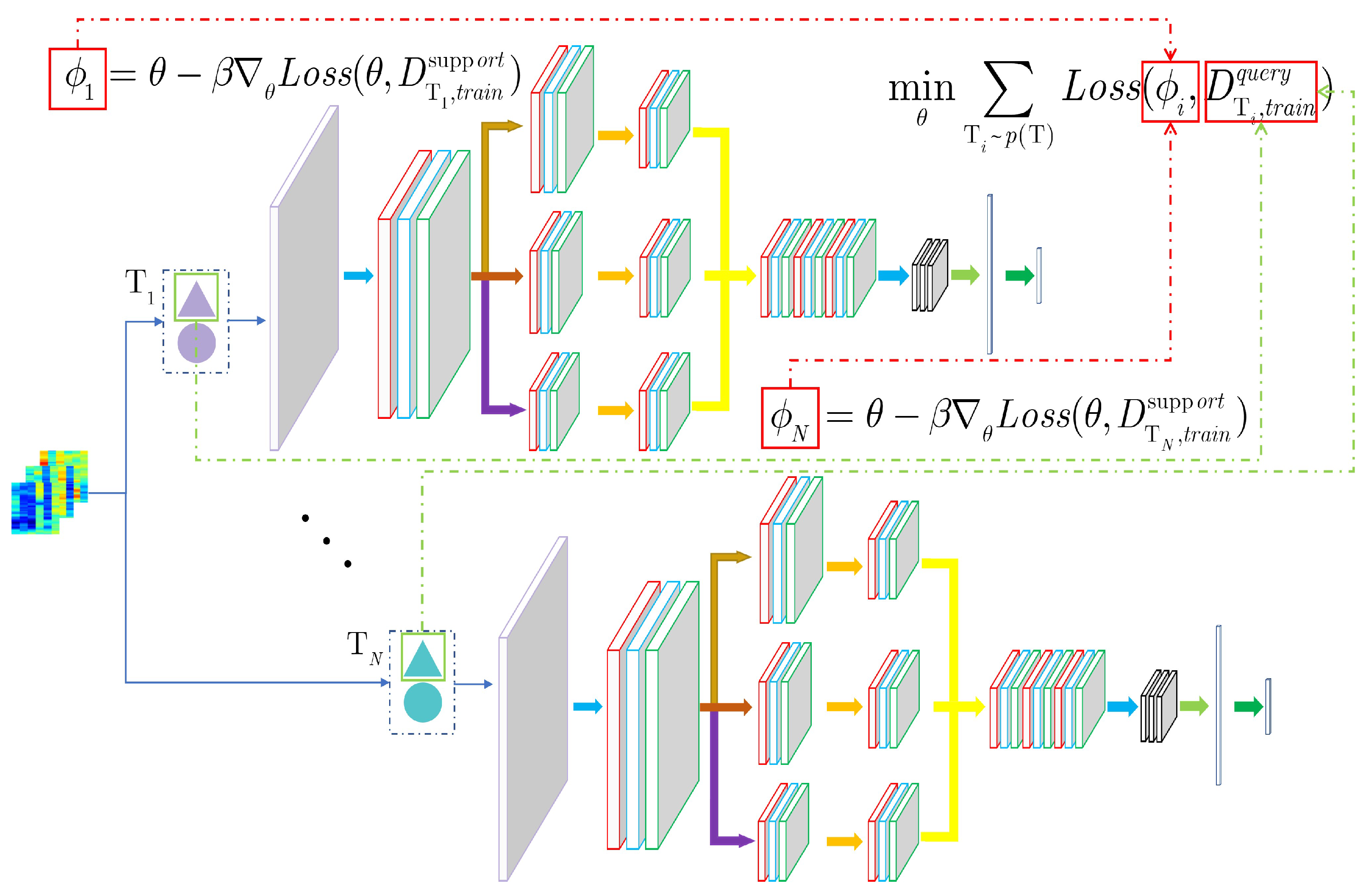
3.3. Meta-Self-Attentive Multi-Scale CNN

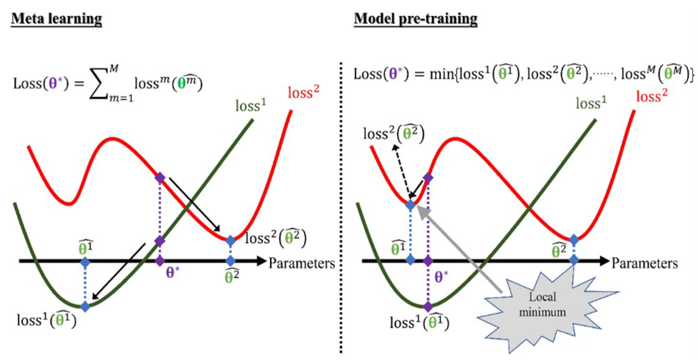
The commonly used methods are meta-learning and transfer learning in cross-domain problems. From the left side of Figure 4, it can be seen that meta-learning summarizes N loss values from N tasks, and then the total loss can be expressed as $loss={\sum }_{n=1}^{N}los{s}^n\left({\widehat{\theta }}^n\right)$. This method takes into account the optimization process of each task. Although the obtained optimal parameter ${\theta }^{*}$ cannot perform well in every task, it can have good generalization capability based on that parameter. A good recognition performance can be obtained by fine-tuning the model with the support set of test samples for each task. The model is trained mainly by obtaining the optimal parameter through the minimum loss function $loss\left({\theta }^{*}\right)=min\{los{s}^1\left({\stackrel{⌢}{\theta }}^1\right),los{s}^2\left({\stackrel{⌢}{\theta }}^2\right),\cdots ,los{s}^N\left({\stackrel{⌢}{\theta }}^N\right)\}$ of the N learning tasks. From the right side of Figure 4, it can be seen that the calculation ${\theta }^{*}$ is only the optimal parameter ${\stackrel{⌢}{\theta }}^1$ for task 1. This will cause the optimization of other tasks to fall into local optimum.

The proposed self-attention multi-scale feature extraction model is described in Section 3.2, which will be trained and learned, since the failure data of autonomous underwater vehicles are very sparse in real-world environments. To cope with the few-shot learning problem, we use a meta-learning strategy to optimize the model. As shown in Figure 1, step 4 aims to generate a meta-deep learning model for generalization to the actual industrial field to implement underwater vehicle actuator fault diagnosis. We need to fit the model through a small number of datasets after establishing the fault diagnosis model, aiming to find the optimal parameters and ensure better performance in the fault diagnosis of underwater vehicles. Thus, the proposed model is trained with the training dataset delineated in step 2 in Figure 1. The training dataset can also be referred to as the source dataset and the test dataset becomes the target dataset; the whole training process is shown in Figure 5.

According to the learning method in Section 2.1, it is necessary to optimize the network by minimizing the objective function, which is expressed as Equation (1).

Expected risk is the global concept that is used to measure the loss of the model concerning the joint distribution $P(x,y)$. Since $P(x,y)$ is unknown, the problem can be transformed into minimizing the expected loss on the training set. The problem then translates into optimizing the model by averaging the losses on the training set, as in Equation (16):

$$R\left(h\right)=R_{emp}\left(h\right)=\frac{1}{N}{\sum }_{n=1}^{N}L(y,h(x;\theta \left)\right)$$

(16)

where $R_{emp}$ is called empirical risk, and this training process is called empirical risk minimization.

In summary, the total error [30] can be decomposed into Equation (19).

$${\epsilon }_{app}\left(H\right)=E[R\left(h^{*}\right)-\underset{f}{argminR\left(h\right)}]$$

(17)

$${\epsilon }_{est}(H,N)=E[R_N\left(h\right)-R\left(h^{*}\right)]$$

(18)

$$E\left[R_N\left(\widehat{h}\right)\right]={\epsilon }_{app}\left(H\right)+{\epsilon }_{est}(H,N)$$

(19)

where the approximation error ${\epsilon }_{app}\left(H\right)$ measures the difference between the predicted and actual values of the few-shot learning model in H. The estimation error ${\epsilon }_{est}(H,N)$ indicates the difference between the estimated and actual coefficients of the model.

The rules for dividing the dataset are shown in Figure 6. We randomly select N subtasks $T=\{T_1,T_2,\cdots ,T_N\}$ from the training set, and the data are divided into the support set and query set in each task $T_i,i\in [1,N]$, represented as $D=\{D^{Support},D^{Query}\}$. Use the support set to complete the iterative optimization of each subtask, and obtain the best parameter ${\theta }^{*}$ by Equation (20), in which i represents the ith task.

$${{\theta }^{*}}^{\left(i\right)}\left(\varphi \right)=argminLos{s}^{task}(\theta ,\varphi ,D_{train}^{Support\left(i\right)})$$

(20)

Using the query set of the training dataset to learn the meta-knowledge, the current optimal parameters ${\varphi }^{*}$ are obtained by Equation (21). Since we are addressing a multi-classification problem, the cross-entropy loss function is used. Equation (22) is the cross-entropy loss function:

$${\varphi }^{*}=\underset{\varphi }{\arg \min }\sum _{i=1}^{N}Los{s}^{meta}({{\theta }^{*}}^{\left(i\right)}\left(\varphi \right),D_{train}^{query\left(i\right)})$$

(21)

$$Loss({\theta }^{*},D^{train})=-{\sum }_{x^{\left(j\right)},y^{\left(j\right)}\in D^{train}}{f}_{{\varphi }_i}\left(x^{\left(j\right)}\right)log\left(y^{\left(j\right)}\right)$$

(22)

where $f_{{\varphi }_i}\left(x^{\left(j\right)}\right)$ represents the trained model, $y^{\left(j\right)}$ represents the sample label, and ${\varphi }_i$ represents the model parameters updated by the ith task.

The performance needs to be tested under the test dataset after the model is fitted under the training dataset. In general, the training data and the test data are from different tasks. Since using the trained model directly on the test set does not work very well, the model parameters are first fine-tuned using the support set of the test dataset. Finally, the model performance is tested using the query set of the test dataset.

$${\theta }^{*}=\underset{\theta }{argmin}(\theta ,{\varphi }^{*},D_{test}^{Support})$$

(23)

For convenience, the above optimization process is organized into a pseudo-code, as described in Algorithm 1.

Algorithm 1: meta-learning strategy

1: while not done do 2: repeat 3:    random sample task $T_i\sim p\left(T\right)$ in total task 4:    for each $T_i$ in $D^{train}$ do do 5:      gain $D_{T_i}^{support}$ by sampling m input-output pairs from $D^{train}$; 6:      evaluate models using cross-entropy loss; 7:      update parameters $\theta$ with gradient optimization of Equation (20); 8:    end for 9:    gain $D_{T_i}^{query}$ by sampling n input-output pairs from $D^{train}$; 10:    update parameters $\varphi$ using $D_{T_i}^{query}$ in Equation (21); 11:    for each $T_i$ in $D^{test}$ do do 12:      gain $D_{T_i}^{support}$ by sampling m input-output pairs from $D^{test}$; 13:      Fine-tuning self-attentive multi-scale model parameters $\widehat{\theta }$ using $D_{T_i}^{support}$ from $D^{test}$; 14:    end for 15:    gain $D_{T_i}^{query}$ by sampling n input-output pairs from $D^{test}$; 16:    test model performance using $D_{T_i}^{query}$ from $D^{test}$; 17: until Accomplish a few-shot fault diagnosis.

4. Experimental Result

4.1. Dataset Introduction

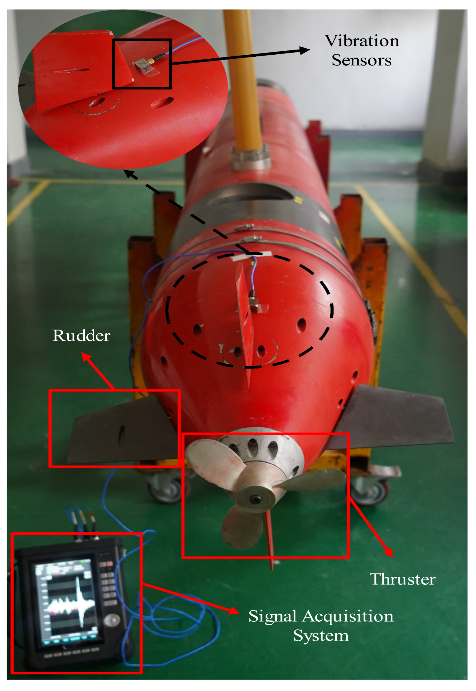
This section uses the vibration data of the AUVs of Northwestern Polytechnical University to verify the proposed actuator fault diagnosis method. Therefore, a high-precision vibration data acquisition experimental platform is established for data acquisition, as shown in Figure 7. The data are divided into rudder vibration data and thruster vibration data, and the sampling frequency is 25,600 Hz. These data are collected in the presence of other device movements, and all data contain noise. Both data types are intended for model training and testing.

The rudder and thruster do not have status feedback in the actual working environment, resulting in an unknown factor regarding whether they operate according to the specified command during operation. Therefore, we need to use the vibration signals to classify the commands of the rudder and thruster, and based on the classification results we can conclude whether the actuator is faulty. The command distribution of the actuator is shown in

Table 2. Distribution of instructions for implementing agencies.

Implementing Agency	Command Distribution	Data Name
Thruster (v)	−1	Thruster 1
	−0.9	Thruster 2
	−0.8	Thruster 3
	−0.7	Thruster 4
	−0.6	Thruster 5
	−0.5	Thruster 6
	−0.4	Thruster 7
	−0.3	Thruster 8
	−0.2	Thruster 9
	−0.1	Thruster 10
	0.1	Thruster 11
	0.2	Thruster 12
	0.3	Thruster 13
	0.4	Thruster 14
	0.5	Thruster 15
	0.6	Thruster 16
	0.7	Thruster 17
	0.8	Thruster 18
	0.9	Thruster 19
	1	Thruster 20
Rudder (°)	0→30→0	Rudder 1
	0→25→0	Rudder 2
	0→20→0	Rudder 3
	0→15→0	Rudder 4
	0→10→0	Rudder 5
	0→5→0	Rudder 6
	0→−5→0	Rudder 7
	0→−10→0	Rudder 8
	0→−15→0	Rudder 9
	0→−20→0	Rudder 10
	0→−25→0	Rudder 11
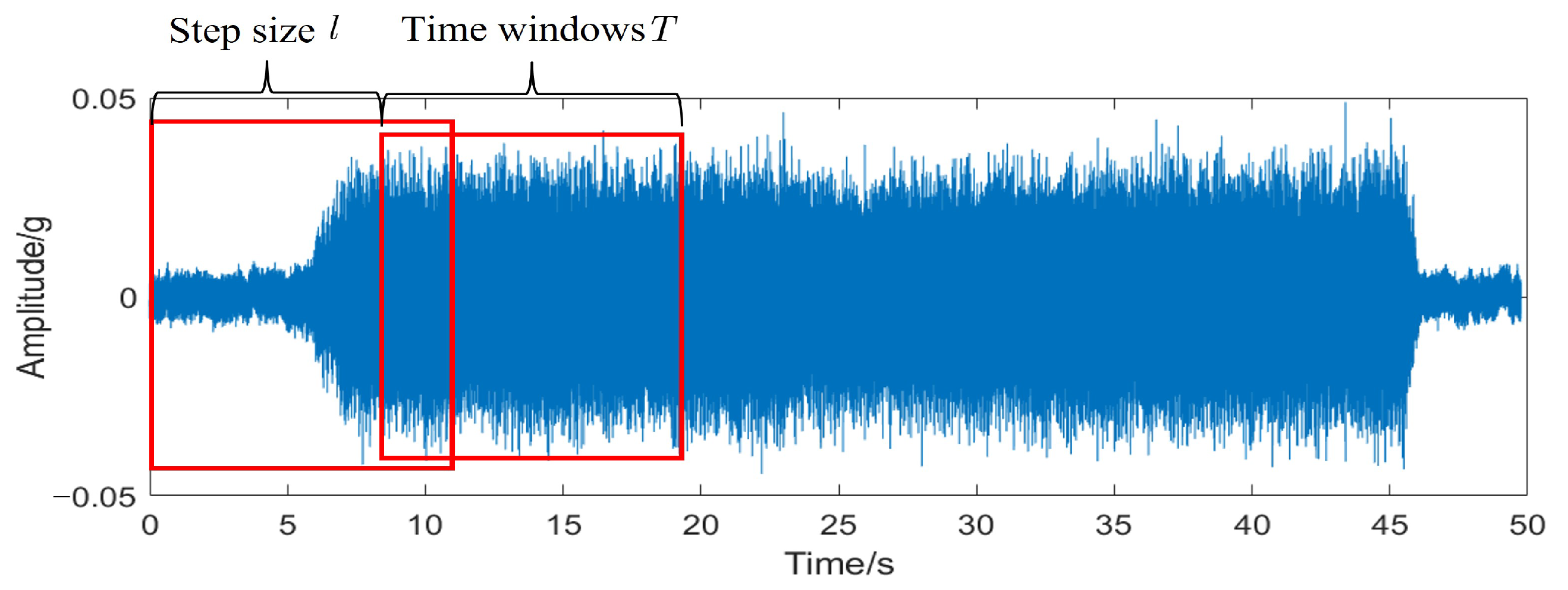
	0→−30→0	Rudder 12

. There are 20 most common commands for thrusters and 12 for rudders, where the minus signs all indicate reverse rotation. To make full use of the vibration data of the actuator, the data are enhanced and resampled in the original data file, using a sliding window with a window size of T and a step size of l. T moves from the start time of the file to the end in step l, and the training and test samples are built. As shown in Figure 8, this article sets T to 2048 and l to 1356.

The typical instructions for the rudder and thruster of the AUV are shown in Table 2 together with the accompanying data files. With the use of these data, we have to produce a meta-training set and meta-test set with various instructions representing various categories, each of which contains some of the samples. The experiment is divided into two cases: Case1 has the thruster as the source domain and the rudder as the target domain; Case 2 has the rudder as the source domain and the thruster as the target domain. The specific dataset partitioning is shown in

Table 3. Divide the data into meta-training sets and meta-test sets.

Datasets		Data File	Number of Samples per Class
Case 1	Meta-training	Thruster	50
	Meta-test	Rudder	50
Case 2	Meta-training	Rudder	50
	Meta-test	Thruster	50

.

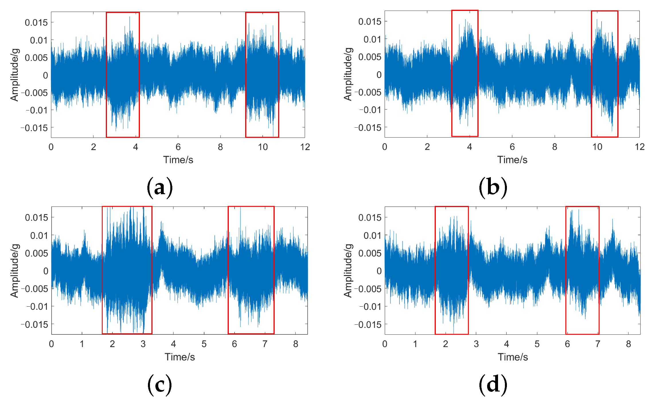
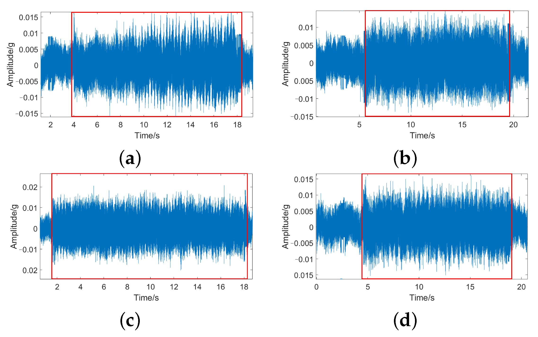
Figure 9 shows part of the time domain waveform of the rudder, which was collected in the operating mode where the rudder and other mechanical devices are operating together. It shows that the vibration signal of the rudder contains background noise, which will be more challenging for the proposed fault diagnosis method. Figure 10 shows part of the time domain waveform of the thruster, where the thruster and the other mechanical devices are also in a commotion mode of operation and the vibration signal contains background noise.

4.2. Benchmark Algorithms

To verify the effectiveness of the proposed actuator fault diagnosis method, four ablation experiments were set up. Both the ablation experiments and the proposed model use the actuator vibration data of the AUVs and are identical except for the different model structures. The following four ablation experiments are presented:

CNN: First, a CNN is used to implement fault detection, and the model consists of two convolutional layers, two pooling layers, two normalization layers, and two fully connected layers. The convolution kernel size of both convolutional layers is 3 × 3.

Multi-scale CNN: The second ablation experiment uses a multi-scale convolutional neural network as a model, consisting of two convolutional layers, two pooling layers, two normalization layers, and two fully connected layers. However, the first convolutional layer no longer uses a single-scale convolution kernel but uses a multi-scale convolution kernel with a convolution kernel size of 3 × 3, 5 × 5, and 7 × 7, respectively. The convolution kernel size of the second convolutional layer is 3 × 3.

Self-attention Multi-scale CNN: Based on the above model, the self-attention mechanism is introduced after the first convolutional layer to further extract more valuable features.

Transfer Network: Based on the above model, the network training is performed using the source domain data, waiting for the model to converge, and then directly using the model for fault diagnosis in the target domain.

Recurrent Neural Networks (RNNs): An RNN classical network with an input layer, hidden layer, and output layer set up to perform fault diagnosis and identification using vibration data from underwater vehicles.

Long Short-Term Memory (LSTM): Based on the RNN network, it changes the way data are transmitted internally by adding input and output gates as well as forgetting gates. This network is used to perform fault diagnosis on the actuators of the underwater vehicle.

4.3. Experimental Results

The previous section introduces the acquisition of datasets, naming of data files, data enhancement operations, and partitioning of meta-training datasets and meta-test datasets using the experimental platform. Then, the meta-training dataset is used to iteratively train the network to converge the model, and the computer software and hardware information used are shown in

Table 4. Main parameters of software and hardware for this study.

CPU	GPU	Memory	Operating System	Deep Learning Architecture
Intel i5-7300HQ	GTX3090	24 GB	Ubuntu 18.04 LTS	Torch 1.11

. The model is fine-tuned using a support set of meta-test data to fit the parameters to the optimal parameters used for the current task. The 100 diagnostic experiments were performed on the query set, mainly to exclude the chance to ensure the generality of the proposed network. The experimental results will be described in detail in Section 4.3.1 and Section 4.3.2.

4.3.1. Case I

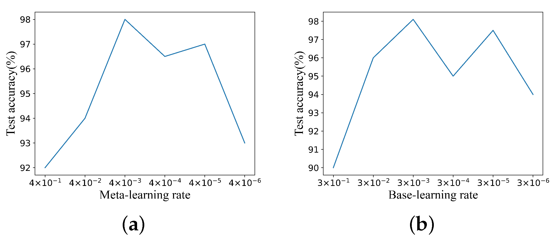
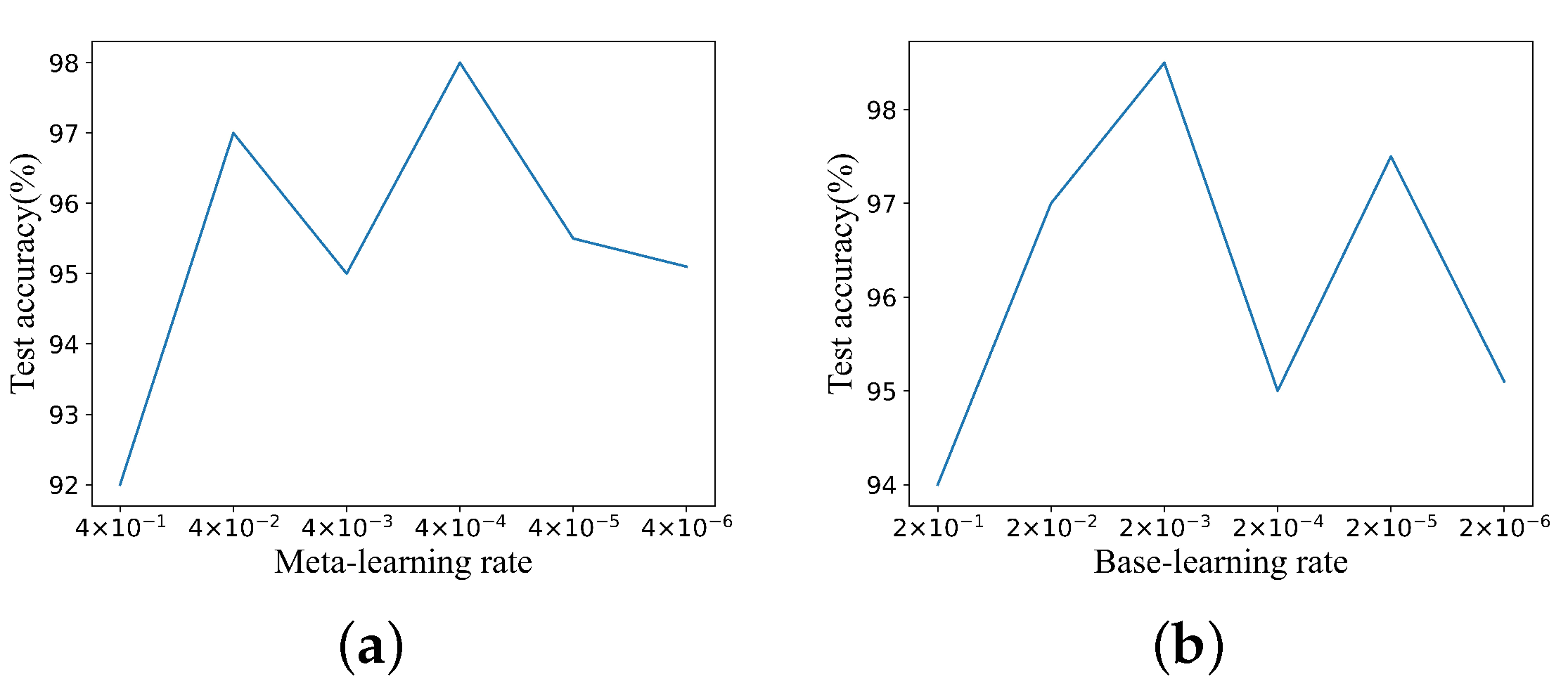
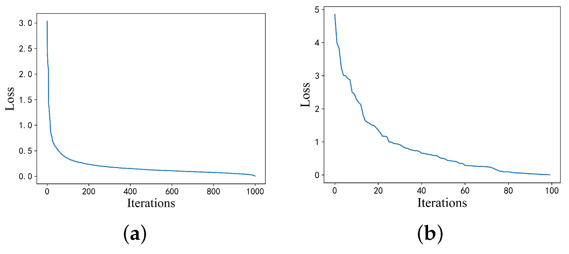
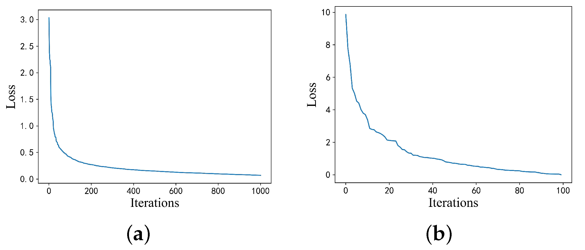
The initial learning rate was discussed and validated by pre-experiments in the diagnostic experiments for Case 1, and the validation results are displayed in Figure 11. Combining the aforementioned findings, $4\times {10}^{-3}$ and $3\times {10}^{-3}$ were chosen as the initial meta-learning rate and initial base learning rate, respectively. The proposed model converged after 1000 iterations on the training dataset. 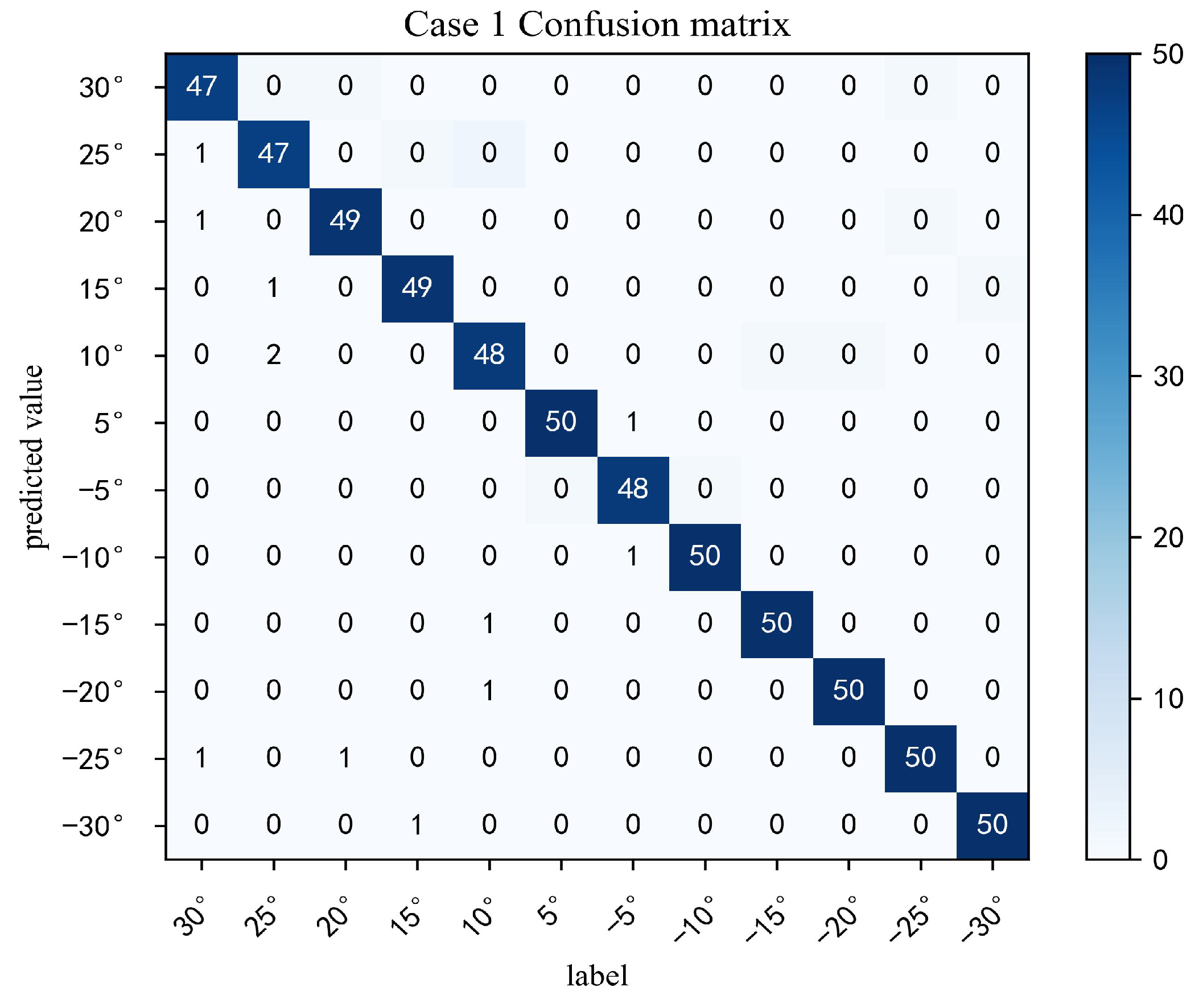The model was then fine-tuned 100 times on the support set of the test dataset, and the loss variation curves of the training and testing processes are shown in Figure 12. A trained model was obtained and tested using the query set of the test set after the fine-tuning of training and testing. From the test results in Figure 13, it can be seen that there are 600 test samples in total, and the number of correctly classified samples is 588, with an accuracy rate of 98%. Among them, the classification accuracy of the six commands 5°, −10°, −15°, −20°, −25°, and −30° was 100%, which produced positive results.

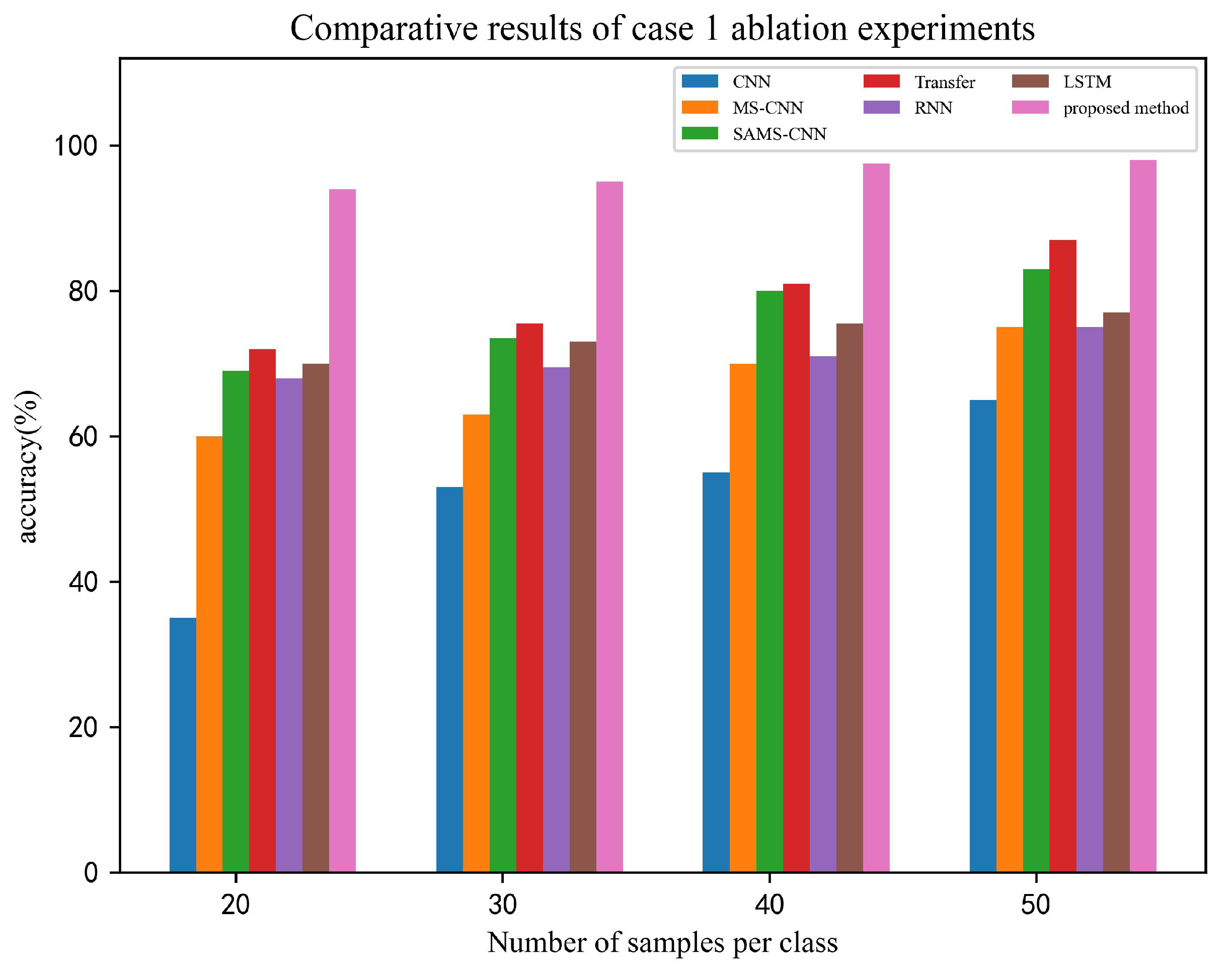
To demonstrate the superiority of the proposed method, six ablation experiments were conducted to classify and identify the vibration data of the underwater vehicle, with the thruster data being the source domain and the rudder data being the target domain. The specific results are shown in Figure 14, which indicates that the proposed method achieves a significant advantage over the other methods. In addressing time-series data, our proposed method outperforms RNN and LSTM, while the recognition ability of the other six methods improves as the number of samples per class increases, but they are still significantly lower than the recognition ability of our proposed method.

4.3.2. Case II

The initial learning rate is discussed and investigated and experimentally validated in the diagnostic experiment of Case 2. According to the results in Figure 15, $4\times {10}^{-4}$, and $2\times {10}^{-3}$ were chosen as the initial meta-learning rate and initial base learning rate, respectively. The loss variation curves of the training process and testing process of the model are shown in Figure 16. A trained network is obtained after training and testing fine-tuning, which is tested using the query set of the test set. 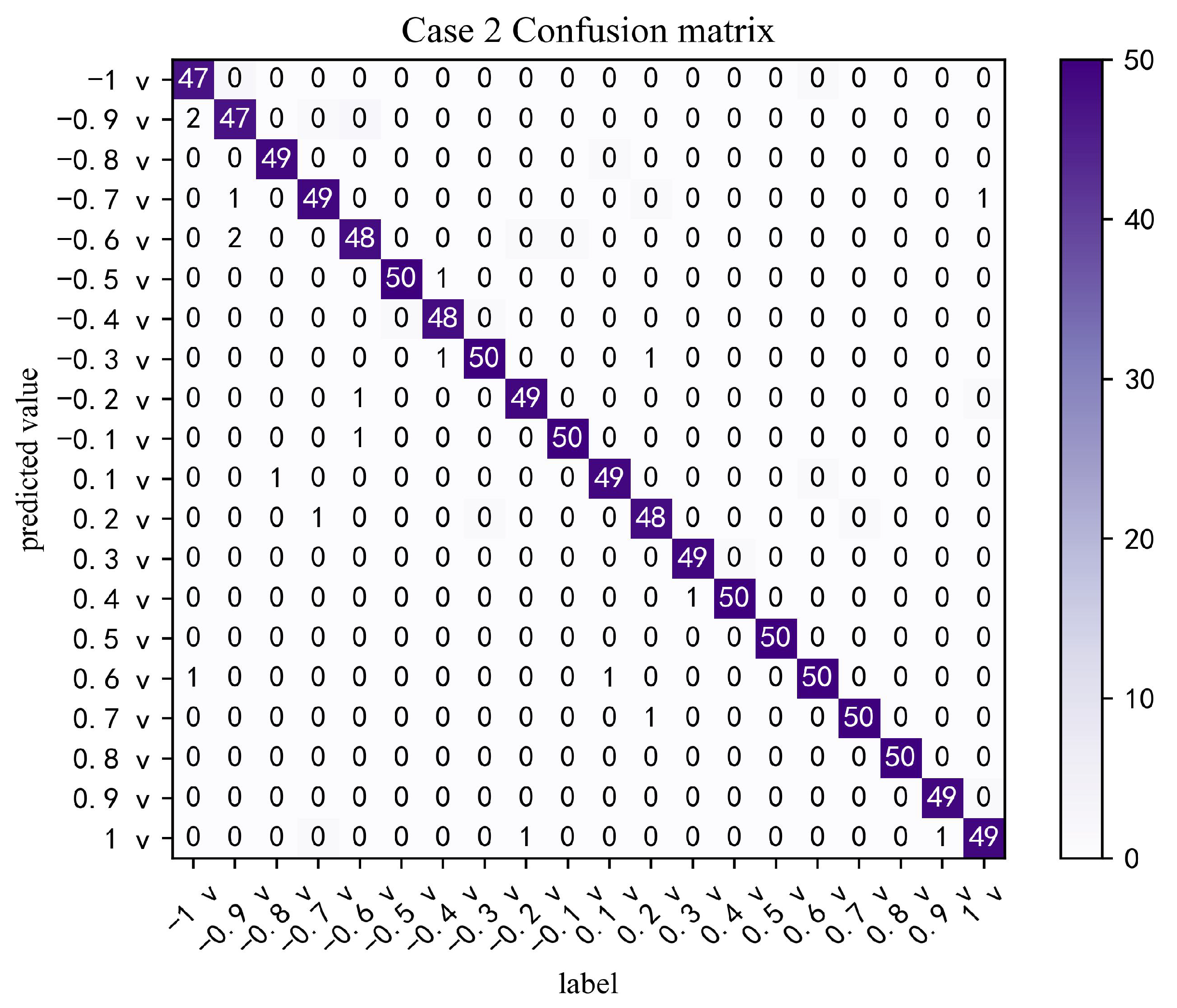From the test results of Figure 17, it can be seen that there are 1000 test samples in total, and the number of correctly classified samples is 979, with an accuracy rate of 97.9%. Among them, the classification accuracy of the eight commands −0.5 v, −0.3 v, −0.1 v, 0.4 v, 0.5 v, 0.6 v, 0.7 v, and 0.8 vs. is 100%, which also produced positive results.

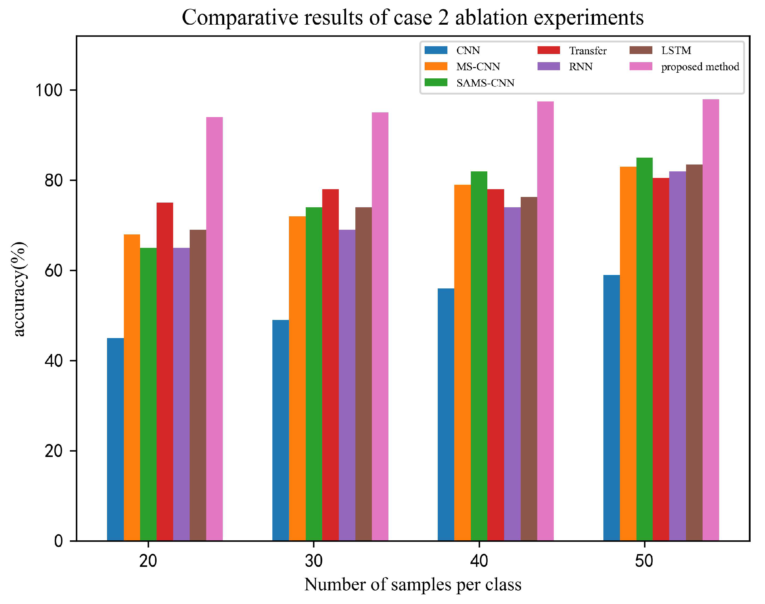
The proposed method’s superiority is demonstrated through six ablation experiments, which aim to classify and identify the vibration data of the AUV, with the source domain being the rudder data and the target being the thruster data. Comparative results of the seven experiments are illustrated in Figure 18, where the proposed method outperforms other methods with a significant advantage. Moreover, the proposed method exhibits better performance in addressing the time-series problem, outperforming RNN and LSTM. Although the recognition ability of the other six methods improves as the number of samples per class increases, they are still significantly lower than the proposed method’s recognition ability. Notably, the proposed method displays less sensitivity to the number of samples, suggesting that it has a distinct advantage in the few-shot problem.

4.4. Discussion of Model Convergence Speed

To demonstrate the rapid convergence property of the proposed method, we compared it with the transfer network, RNN, and LSTM architectures set up in Section 4.2. All variables, except for the network model, were kept consistent and convergence time was utilized as the performance metric for comparison. We conducted the experiments on a computer with the same hardware configuration and used the thruster data as the source domain data and the rudder data as the target domain data. 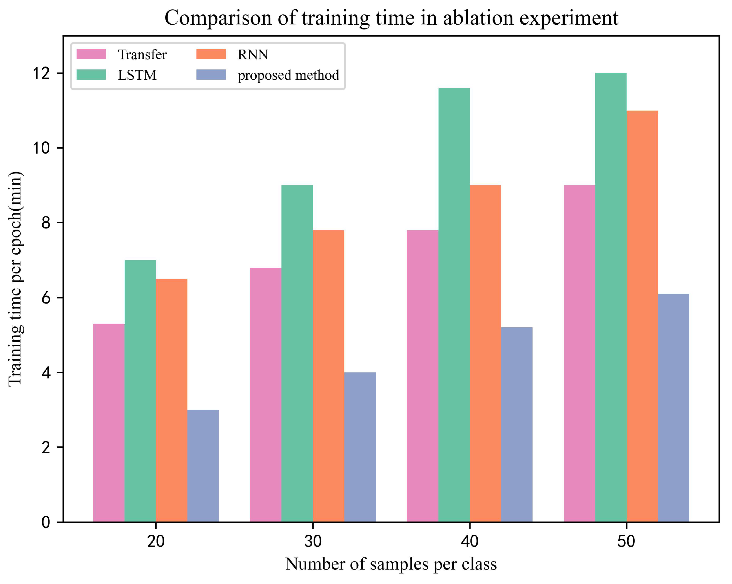The specific results are shown in Figure 19.

Based on the experimental results, it is evident that the proposed method requires the shortest amount of time for each training round, while the LSTM model takes the longest time. This can be attributed to the fact that the proposed method is a shallow model with fewer training parameters, which allows it to learn the optimal parameters more rapidly. Moreover, as highlighted in Section 4.3, the proposed method exhibits fast convergence and superior recognition performance.

5. Conclusions

In this paper, we propose the MSAMS–CNN fault diagnosis method, which can accomplish the fault diagnosis task of autonomous underwater vehicle actuators. Both self-attentive mechanisms and multi-scale approaches are used in extracting vibration data features to ensure that the extracted features can characterize the actuator fault states. Additionally, we utilize a meta-learning training and testing strategy to fit and evaluate the proposed model, effectively overcoming the issue of a limited AUV actuator dataset. Furthermore, the convergence speed of our method is faster in comparison to other approaches. The trained model demonstrates favorable generalization ability and is proficient in accomplishing cross-target fault diagnosis tasks. Experimental results show that the method outperforms the set up ablation experimental model in terms of diagnostic accuracy. In the future, the network needs to be further investigated and improved to enhance the model fitting speed and accuracy and to reduce the dependence on the computer hardware configuration.