Article

A Novel Short-Term Ship Motion Prediction Algorithm Based on EMD and Adaptive PSO–LSTM with the Sliding Window Approach

Key Laboratory of Advanced Marine Communication and Information Technology, College of Information and Communication Engineering, Ministry of Industry and Information Technology, Harbin Engineering University, Harbin 150001, China
*
Author to whom correspondence should be addressed.
J. Mar. Sci. Eng. 2023, 11(3), 466; https://doi.org/10.3390/jmse11030466
Submission received: 19 January 2023 / Revised: 12 February 2023 / Accepted: 15 February 2023 / Published: 21 February 2023
(This article belongs to the Section Ocean Engineering)

Abstract

:
Under the influence of variable sea conditions, a ship will have an oscillating motion comprising six degrees of freedom, all of which are connected to each other. Among these degrees of freedom, rolling and pitching motions have a severe impact on a ship’s maritime operations. An accurate and effective ship motion attitude prediction method that makes the prediction in a short period of time is required to guarantee the safety and stability of the ship’s maritime operations. Traditional methods are based on time domain analysis, such as the autoregressive moving average (ARMA) models. However, these models have limitations when it comes to predicting the nonlinear and nonstationary characteristics of real ship motion attitude data. Many intelligent algorithms continue to be applied in nonlinear and nonstationary ship attitude prediction, such as extreme learning machines (ELMs) and the long short-term memory (LSTM) neural network, as well as other deep learning methods, showing promising results. By using the sliding window approach, the time-varying dynamic characteristics of the ship’s motion attitude can be preserved better. The simulation results demonstrate that the proposed model performs well in terms of predicting the nonlinear and nonstationary ship motion attitude.

1. Introduction

Under the influence of wind [1], waves [2], and other environmental elements, the six degrees of freedom comprising the swaying motion of large ships can become complicated and uncertain [3]. These factors represent a threat to ships’ offshore operations, especially in complex environments. Methods for the short-term prediction of a ship’s motion attitude have been proposed to predict the offshore motion of ships in the next few seconds in real time. Such methods provide decision-making information for the accurate control of a ship’s offshore operations and the selection of the optimal operation time to enhance the safety and efficiency of the offshore operations. In general, there are four types of models for predicting a ship’s motion: physical models based on the ship’s hydrodynamic coefficients and equations, statistical models based on historical data and future data, intelligent models based on time series analysis and intelligent algorithms [4,5], and hybrid models [6,7].
Methods for the short-term prediction of a ship’s motion attitude that were based on linear hydrodynamic motion equations were extensively used in early research. In 1969, Kaplan [8,9] designed a Wiener filter based on the statistical parameters of a ship’s motion power spectrum to predict the ship’s short-term motion. However, this method has the disadvantages of calculation complexity and low accuracy. With the development of modern control theory, a method for the short-term prediction of a ship’s motion attitude based on the Kalman filter was proposed to predict it in real time [10]. However, the accuracy and stability of the prediction method based on the Kalman filter cannot meet the necessary requirements, especially in severe sea environments.
The methods for the short-term prediction of a ship’s motion attitude are based on the time domain analysis approach, which is a data-driven prediction method. It only requires the historical data of a ship’s motion to establish a time series model to predict the ship’s extremely short-term attitude. However, methods, such as AR and ARMA, require the ship’s motion data to be stationary and linear, which is unsuitable for realizing good prediction results of the nonlinear or nonstationary characteristics of the ship’s motion [11]. In the past few years, methods for the short-term attitude prediction of a ship’s motion based on machine learning (ML) models have become very popular in the context of nonlinear or nonstationary characteristics [12,13,14,15,16,17,18,19]. These data-driven prediction methods have gained more attention due to their superior capabilities of learning and modeling complex nonlinear relationships, including artificial neural networks (ANNs) [20], recurrent neural networks (RNNs) [21], support vector machines (SVMs) [22,23], random forest (RF) [24], multi-layer perceptron (MLP) [25], feed-forward neural networks (FNNs), back-propagation neural networks (BPNNs), and extreme learning machines (ELMs) [26,27,28]. Of these, RNNs memorize the previously known information and pass this to the input, which ensures the relation among the input information and achieves good prediction results, especially for periodic sequences. However, relying solely on the above intelligent models may not meet the practical requirements for an accurate prediction. Furthermore, there are some limitations and considerations to be aware of when using a single machine learning model to predict a ship’s motion:
  • Due to having less generalization ability, a single neural network encounters the problems of over-fitting, vanishing gradients, and network training explosions when faced with the complex patterns in a ship’s motion dataset.
  • When dealing with huge datasets, simple neural network models may become unstable and have low efficiency.
To overcome the shortcomings of ML methods, researchers have been inspired to develop a promising methodology: deep learning (DL). DL, as a branch of ML, trains the data model by utilizing multiple processing layers at multiple levels [29]. The performance of DL models is improved by increasing the number of hidden layers, while the deeper architecture increases the number of parameters to be optimized, which further increases the training time of the model. The potential of DL in applications requiring predictions has been highlighted in the recent literature. For time series forecasting, DNN models, such as long short-term memory (LSTM), gated recurrent units (GRUs), and hybrid models have proven to be both powerful and accurate tools. Currently, researchers are considering hybrid models to enhance the performance of DL models. Qin et al. proposed AR-DWT-EMD to solve the problem of the prediction of the nonlinear and nonstationary motion of ships [30]. In [31], the decomposition and the Hilbert spectrum of the inputs (sea waves) were compared with the decomposition and the Hilbert spectrum of the outputs (ship movements, generated by the waves) to study the time–frequency characteristics of the ship’s response. However, we mainly focused on the decomposition of the original nonstationary time series to decrease the effect of noise. The decomposition extracts the important features to improve the accuracy of the prediction. EMD can adaptively perform time–frequency localization analysis to effectively extract the characteristic information of the original signal. Wang et al. proposed the Bi-LSTM TPA hybrid model, which extracts the time features from both the forward and reverse roll angle time series to improve the prediction of the ship’s roll angle [32]. Additionally, hyperparameter inference and optimization procedures in neural networks, such as ant colony optimization [33], PSO [34], and the genetic algorithm [35], are used to improve the prediction performance. Yin et al. proposed a scheme for predicting rolling based on an adaptive sliding window considering the characteristics of the ship’s rolling motion. An online experiment on the prediction of the ship’s rolling was conducted to verify the effectiveness of the adaptive sliding window [36]. In [37], the simulation results showed that the combination of LSTM and PSO improved the accuracy of the prediction of the ship’s motion. Z. Nie et al. conducted a simulation experiment on the prediction results of support vector regression (SVR) algorithms based on four commonly used kernel functions and compared the effectiveness and practicality of these kernel functions in the prediction of the ship’s motion [38]. Zeguo Zhang et al. proposed a prediction algorithm based on GPSO-ANFIS and applied it to the real-time prediction of the ship’s rolling. The simulation results showed the advantage of the method regarding its accuracy, stability, and real-time performance [39]. In summary, the following issues need to be noted for the short-term prediction of a ship’s motion:
  • To complete the short-term prediction, a few seconds of ship motion attitude data are derived by the proposed model.
  • The sliding window technique is introduced to turn time series predictions into supervised learning for ML methods. Each window is utilized to train and update the model. After each computation is completed, the window shifts to a new position by one step.
  • Because of the nonstationary characteristics of time-series data, the prediction accuracy is affected by the unstable mean and variance of datasets. Therefore, to obtain better prediction results, the present work needs to use a data pre-processing method to reduce the effect of nonstationary characteristics.
  • Considering the practicality of predictive models, the proposed model needs to guarantee high-accuracy results when faced with multi-step-ahead predictions.
In this paper, aiming to reduce the nonlinear and nonstationary ship motion characteristics and obtain the optimal parameter of the neural network, a hybrid multi-step prediction model is proposed by combining the LSTM model with EMD, and adaptive PSO is proposed to predict ship motion attitude in a few seconds. The EMD method is employed for dealing with nonlinear and nonstationary time series, and the LSTM approach is used for training and predicting the derived ship attitude, while the parameter optimization algorithm based on PSO is utilized to maximize the performance of the prediction model by adjusting the parameters of the LSTM neural network. Additionally, time series datasets can be framed into supervised learning for multi-step predictions by utilizing the sliding window technique.
The rest of this paper is organized as follows. Section 2 gives a brief description of EMD and the sliding window approach. In Section 3, the hybrid ship attitude prediction model is established by EMD and the LSTM neural network with the sliding window approach. In Section 4, the proposed model is implemented in a real-time ship motion attitude data experiment, and the model’s performance is tested using at different datasets. Conclusions are derived in Section 5.

2. Basic Knowledge

2.1. Empirical Mode Decomposition Method

Affected by various random and uncertain factors, noise exists in the measured ship motion data and interferes with the valid signals. It overlays and obscures the best-expected results when processing the original observation data. Therefore, it is crucial to apply denoising techniques to the raw data prior to the ship motion attitude prediction processing in order to enhance the accuracy of the subsequent forecast. EMD decomposes the signal into a finite number of eigenmode functions (IMFs), discards the noisy IMFs, and reconstructs the remaining IMFs to denoise the raw data. Since EMD is based on the time-scale characteristics of the data itself and does not require a given basis function in advance, it has obvious advantages when dealing with nonsmooth and nonlinear time series. The process of decomposition involves the following steps:
  • Find all maximum and minimum points of the time series x ( t ) and then fit a curve with a cubic spline function to obtain the upper and lower envelope of x ( t ) , which can be represented, respectively, as u ( t ) and l ( t ) .
  • Calculate the average of u ( t ) and l ( t ) to obtain the mean envelope m x , which is shown as Equation (1):
    m x = u ( t ) + l ( t ) 2 .
  • New time series h x can be calculated as
    h x = x ( t ) m x .
  • Judge if h x is satisfied with the condition of IMFs. Repeat Steps (1), (2), and (3) if it is not satisfied until the mean envelope tends to zero. Then, the first intrinsic modal function i m f 1 is obtained.
  • By subtracting i m f 1 from the original time series x ( t ) , the new time series r x 1 without high frequency is derived.
  • By repeating the above process, the intrinsic modal function i m f 2 , i m f 3 , , i m f n is obtained. When the r x n cannot be decomposed, it is represented as the residual of x ( t ) .
After the above steps, the original time series x ( t ) can be represented as
x ( t ) = i = 1 n i m f i + r x n ,
where r x n represents the trend of x ( t ) , and it is without a high-frequency component.
During the whole process of EMD, one of the cyclic processes is the shifting process in which the optimal time of shifting and decomposition needs to be considered. Additionally, the two termination criteria include the component termination condition and the decomposition termination condition.
The shifting is the process of obtaining the IMF component, and the basic method is to continuously find extreme points from the original signal and continue shifting according to the decomposition steps until a certain condition is met. The purpose of this process is to reduce the asymmetry of the signal so that the waveform tends to be symmetric around the zero mean line, so as to meet the basic characteristics of the component. Additionally, the instantaneous frequency can be calculated by transformation. In order to ensure that the components obtained by the decomposition have sufficient original physical significance of frequency modulation (FM) and amplitude modulation (AM), the number of shifting cycles should not be excessive. Too many cycles will over-smooth the component and make it a constant amplitude FM signal, which loses the original physical meaning. On the other hand, too few shifting cycles will make the resulting component not entirely meet the basic characteristics of the component and do not obtain accurate instantaneous and meaningful frequency.

2.2. Sliding Window Approach

A sliding window is a fixed-size window that will circle the values around a point in the time series to obtain an interval that is used to calculate statistical indicators for data of a specified length. The sliding window width has an immediate effect on the model prediction. The window length is used to weigh the amount of input data and the length of historical information included. However, too much input data will lead to complex calculations and slow down the training of the neural network. Less input data tend to include less historical information, making it difficult to reflect the cycle pattern. The application of the sliding window technique in multi-steps is shown in Figure 1.
Datasets can be framed into supervised learning for prediction by sliding windows, and data from each window are utilized to train and update the model. After completing each computation, the window shifts to the next new position.
Since the selection of the key parameters of LSTM has a great influence on the accuracy of ship motion attitude forecasting, these parameters need to be selected reasonably. The particle swarm optimization (PSO) algorithm has the advantages of simple structure, high precision, fast convergence speed, and ability to deal with nonlinear and multivariable problems, which are effective tools for the selection of LSTM model parameters.

3. Short-Term Ship Motion Prediction Algorithm based on EMD and Adaptive PSO–LSTM

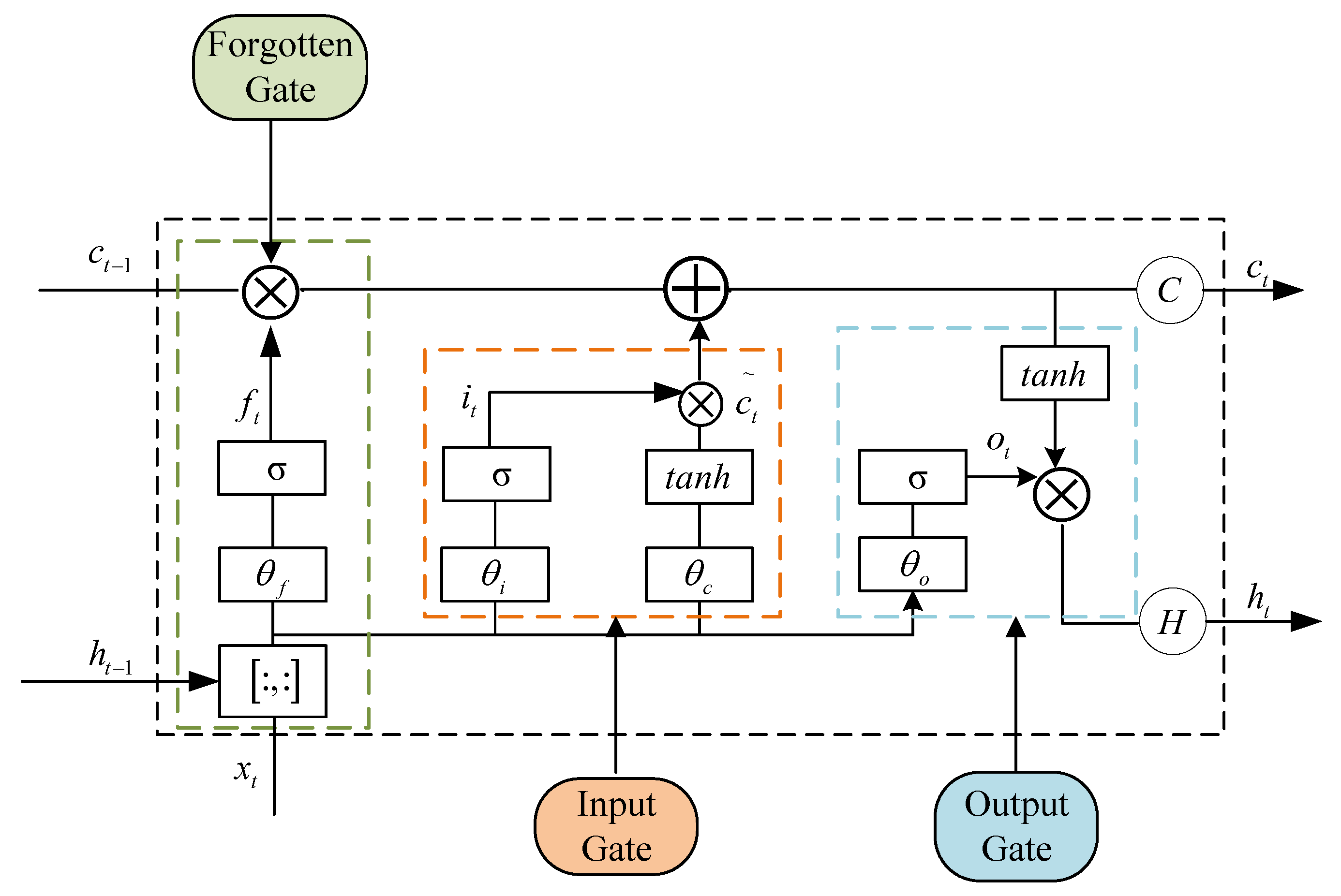
3.1. LSTM Neural Network Parameter Optimization for Ship Attitude Prediction

The long short-term memory (LSTM) neural network, which is a novel recurrent neural network, was proposed by Hochreiter and Schmidhuber [40]. As a deep learning model, LSTM learns the pattern from historical data accurately by utilizing the selective memory capability of machine learning and digging into the intrinsic patterns of known time series to achieve its short-term forecasting of time series. The advantage of LSTM is to solve the problem of gradient disappearance compared with other types of recurrent neural networks by introducing the concept of state units and gates into the neural network. As a result, it has better adaptability in data analysis compared with the RNN network. The structure of the LSTM unit is shown in Figure 2:
Each neural unit contains three gate control structures which are forgotten gate, input gate, and output gate. The selective transmission of data information is controlled by these gates, and the output of the sigmoid layer is a value between zero and one, which describes the ratio of information transmission. The valid information at the last epoch in f t is discarded and retained by the forgotten gate. Current valid information i t is stored in the input gate, which determines the update of the cell state. The output layer determines the information that needs to be output as o t in the LSTM neural unit. The output value of the hidden layer h t and the unit state c t at the current epoch are determined by the output value of the hidden layer at the previous epoch h t 1 , the unit state c t 1 , and the input value at the current epoch x t .
Since the input is determined by the output of the previous epoch h t 1 , the input of the network at the current epoch x t and the activation function sigmoid control the information transfer ratio. The calculation process of the forget gate is shown as follows.
f t = σ ( W f h t 1 + U f x t + b f ) ,
where W f and U f represent the weight matrix, b f denotes the bias term, and σ is the activation function. Since the input of the sigmoid function is determined by the output at the previous epoch h t 1 and the input of the network at the current epoch x t , the calculation process of the input gate is shown as follows.
i t = σ ( W i h t 1 + U i x t + b i ) ,
where i t represents output, W i , U i represent the weight matrix, and b i denotes the bias term. The tanh function is utilized to update the cell state and create a new candidate vector in the input gate. Then, the input of the memory cell c ˜ t is obtained as follows:
c t ˜ = tanh ( W c h t 1 + U c x t + b c ) ,
where W c , U c represent the weight matrix, and b c is the bias term. Since the input is determined by the output of the previous moment h t 1 and the input of the network at the current moment x t , the output of gate o t is obtained from the activation function sigmoid. The output gate is calculated as follows.
o t = σ ( W o h t 1 + U o x t + b o ) ,
where W o , U o represent the weight matrix, and b o denotes the bias term. We combine the partial information retained in the forget gate with the input gate to form a new cell unit c t as follows.
c t = f t c t 1 + i t c t .
Next, c t will be sent to the tanh function through the output gate to determine the output value of the hidden layer at the current epoch h t , which can be derived by h t = o t tanh ( c t ) , where ⊙ denotes the element-wise vector product. In general, LSTM includes two kinds of hidden states: a slow state c t to solve the vanishing gradient problem and a fast state h t to make complex decisions over short periods of time.
The PSO algorithm is an appropriate method for parameter selection in the LSTM model, thanks to its benefits, such as straightforward structure, high accuracy, fast convergence rate, and the capacity to address nonlinear and multivariable problems. PSO describes the members of the group as particles, and the fitness of all particles is determined in space through a fitness function. In the early stage of evolution, both the position and speed of each particle are initialized randomly. The particles cooperate with each other during the flight and adjust their speed and positions in time according to the motion state of themselves and their companions in order to land on a better position. However, each particle is a solution of the solution space in PSO. Each particle knows its own position and the information of other particles. It adjusts its position and speed through its optimal position and area of the group, and then the global optimal solution is derived. The speed and position of the PSO are updated as follows:
v i , j t + 1 = w v i , j t + c 1 r 1 ( y i , j t x i , j t ) + c 2 r 2 ( y j t * x i , j t ) ,
x i , j t + 1 = x i , j t + v i , j t + 1 ,
where w is the inertia weight, c 1 and c 2 are learning factors, r 1 and r 2 are independent random numbers distributed between zero and one, and v i , j t , x i , j t , y i , j t , and y j t * are the velocity component, position component, individual optimal value, and group global optimal value of the i-th particle in the j-th dimension in the t-th iteration, respectively.
The value of w affects the model’s optimization ability. In order to avoid premature convergence of the model, an adaptive PSO method is adopted in this paper. It adaptively adjusts the inertia weight as follows.
w = w min ( w max w min ) ( f f min ) f a v g f min , f f a v g w max , f > f a v g ,
where w max , w min are maximum and minimum of w, respectively; f is the current fitness value of the particle; f min and f a v g represent the current minimum fitness of all particles and the average fitness value, respectively.
Since ship motion data have the characteristics of instability, nonlinearity, and periodic uncertainty, an adaptive PSO–LSTM is proposed in this paper. In the novel model, an adaptive PSO is utilized to optimize the network hyperparameters. The whole process of the adaptive PSO–LSTM method is shown as follows.
  • Preprocess the ship historical movement data.
  • Initialize the particle swarm parameters, including the determination of the population size, number of iterations, learning factors, and limited intervals for particle position and velocity.
  • Initialize the LSTM network structure, which refers to the determination of the number of neurons in each layer of the network and the number of hidden layers. It also divides the data into training samples, validation samples, and test samples.
  • Determine the fitness function and select the optimal particle fitness value by calculating and comparing the fitness value of each particle. The fitness value f i t i of population individuals x i with LSTM model parameters is defined as Equation (12).
    f i t i = 1 2 ( 1 M m = 1 m y m y m y m + 1 N n = 1 n y n y n y n ) ,
    where M and N represent the number of training samples and verification samples, respectively; y m and y m represent the true value and the prediction value of the training sample, respectively; y n and y n represent the true value and the prediction value of verification samples, respectively.
  • Calculate and evaluate the particle fitness value according to the difference of the particle fitness value. The global optimal position and the local optimal position of the particle are both determined.
  • Update the velocity and position of the particles based on Equations (9) and (10).
  • Determine whether the particles meet the conditions for the iteration termination. If the maximum number of iterations is reached, the optimal parameters are assigned to the LSTM, and the training is performed and outputs the short-term ship motion prediction value. Otherwise, it returns to Step 5 to continue execution until the termination condition is met.
  • The optimal results obtained are assigned to the connection weights of the LSTM network, and this prediction model is trained to output the optimal solution for time series prediction.
The flowchart of the adaptive PSO–LSTM method is shown in Figure 3.
Most previous studies have only used the fitting error of the training sample as the fitness value and ignored the effect of the testing sample data, which results in over-fitting in the neural network. This leads to the model prediction result not being optimal. Therefore, the fitting error of the training sample and the verification error of the verification sample should be considered in the fitness function.

3.2. EMD–LSTM Model Based on Sliding Window Approach

The ship motion time series is regarded as a nonlinear signal sequence. EMD has certain advantages in dealing with the end effect and reducing the effect of system noise. Therefore, it was selected to decompose the original sequence before prediction, which improves the model’s fitting performance. This part of the prediction is based on the LSTM neural network with the sliding window. The adaptive PSO is used to optimize the value of network hyperparameters in the LSTM model, which cannot be selected objectively and scientifically. As a result, the whole process is summarized as follows:
  • Decompose the raw ship motion sequence into multiple specific subsequences by utilizing the EMD algorithm.
  • Divide the dataset into the training set and the testing set and predict each sub-model component separately with a sliding window and optimized LSTM neural network.
  • Weight and reconstruct the prediction of each sub-model to obtain the final prediction results.
The flowchart is shown in Figure 4:

4. Experiment Results and Analysis

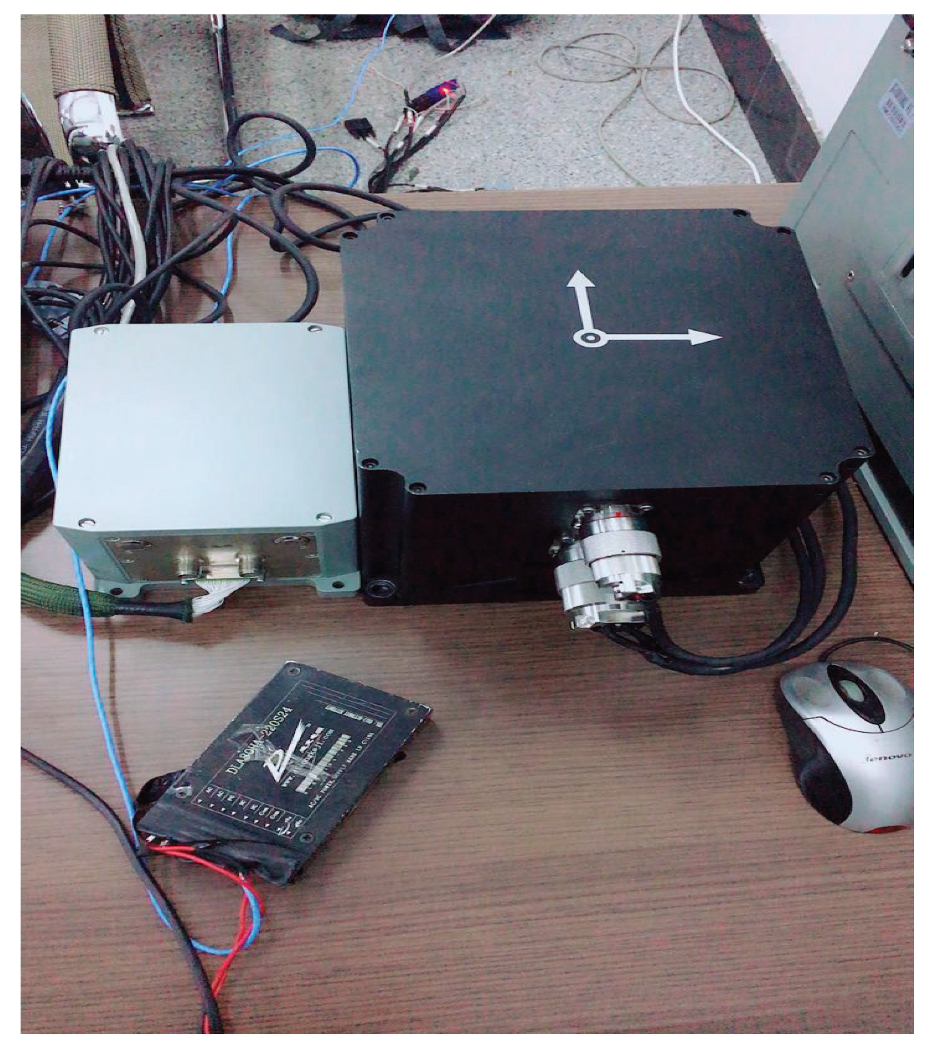
4.1. Experiment Design and Parameter Settings

Experiments were conducted to verify the effectiveness of the prediction model proposed in this paper. The experimental data used in this study were collected from an inertial measurement unit (IMU) installed on a large ship and divided into two categories in total: static state data set and motion state data set. The “static state” and “motion state” represent the state of the ship when we measured the experimental data of ship attitude. “Static state” means that the ship is docked at the port. “Motion state” means that the ship is sailing at a certain speed. To ensure the reliability and accuracy of the proposed algorithm, it was necessary to select the datasets in different states and different timestamps. The detailed description of the datasets is shown in Table 1. The sampling frequency of the IMU was 4 Hz. The scene of raw data acquisition is shown in Figure 5. The first 80% of the data was used for training and the rest was used for testing. Figure 6, Figure 7, Figure 8, Figure 9 and Figure 10 show the different datasets of raw roll angle and pitch angle of the ship.

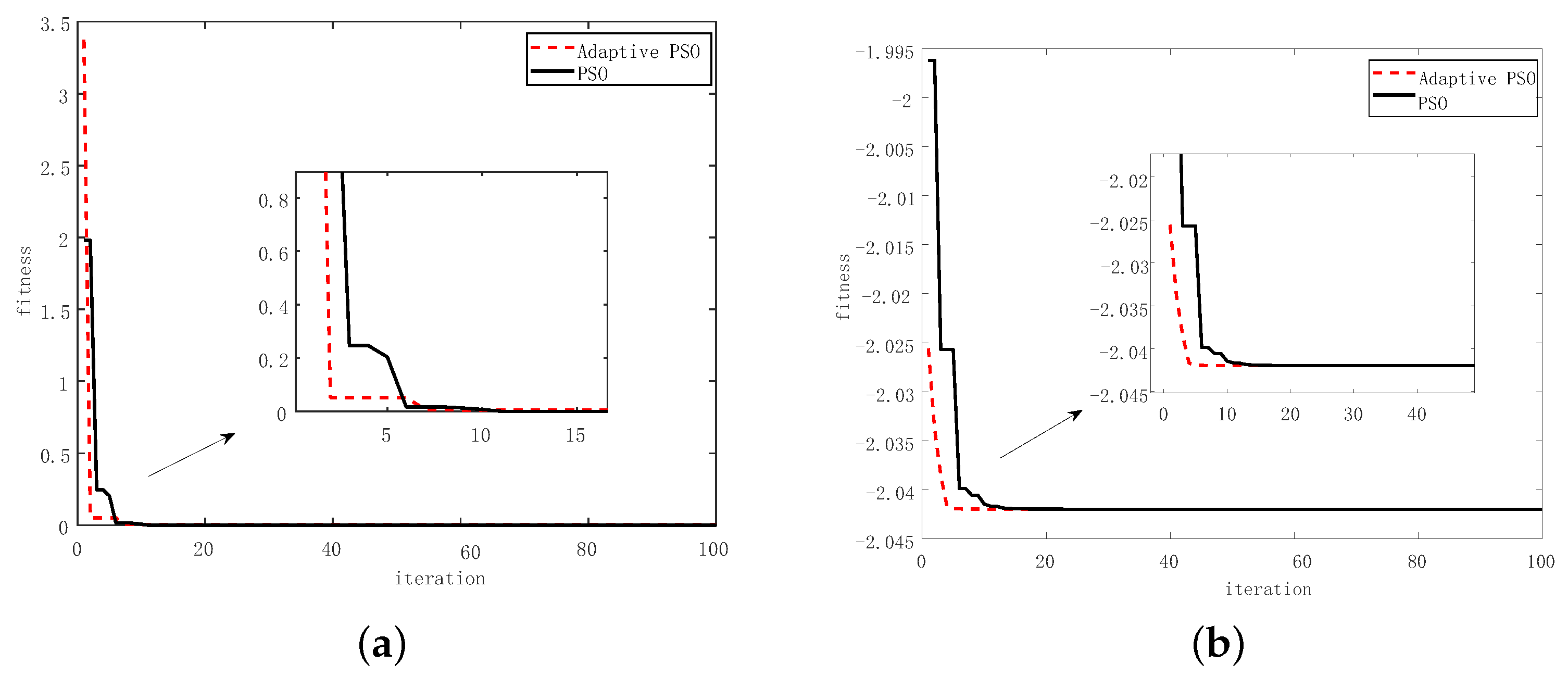
4.2. Prediction Performance Evaluation of Adaptive PSO Algorithm and Hybrid Model

To test the performance of the adaptive PSO algorithm, two standard test functions were chosen for both PSO and adaptive PSO. The two functions are expressed in Table 2.
The Griewank function has local minima, the number of which is related to the dimensionality of the problem, and the minimum is obtained at (0, 0 …0). It is a nonlinear multimodal function with a very wide search space and can be used to test particle swarm algorithms.
The Rosenbrock function is a nonconvex function used to test the performance of the optimization algorithm. Each contour of the Rosenbrock function is roughly parabolic in shape, and its full-domain minimum is also located in a parabolic-shaped valley (a banana-shaped valley). It is easy to find this valley, but it is quite difficult to find the minimum value of the full domain because the values within the valley do not vary much. Its full domain minimum is located at the point ( x , y ) = ( 1 , 1 ) with the value f ( x , y ) = 0 . Sometimes, the coefficient of the second term is different, but it does not affect the location of the full domain minimum.
The parameters in PSO and adaptive PSO were set as follows. The maximum population size was 100; the maximum number of iterations was 100; maximum particle velocity V max = 5 ; learning factors were set as c max = 2.1 , c min = 0.8 ; and inertia weight was w max = 0.9 , w min = 0.4 , respectively. Figure 11 indicates the optimization results of the above test functions. It is obvious that the adaptive PSO algorithm showed better performance in finding the best individual fitness with less iteration and faster convergence.
The ship motion varies greatly due to the environment at sea. Dense and highly fluctuating data may obscure the less fluctuating parts, resulting in missing details. Therefore, the data need to be normalized to eliminate the dimensional difference between different dataset inputs and scale them according to a certain ratio within the set interval. Both the sample set and target set should use the same normalization standard to ensure the consistency of neural network training and prediction. The formula of normalization is as follows:
X N = x i x min x max x min ( b a ) + a ,
where X N is normalized data, x max and x min represent max and minimum of the data sequence x i , respectively. Here, x i can be set from a to b. It is set in the range from 0 to 1 in this paper.
Once the ship motion prediction is completed, it needs to be de-normalized, as indicated in Equation (14):
x i = ( x max x min ) X N + x min .
Mean absolute error (MAE), mean absolute percentage error (MAPE), and root mean square error (RMSE) were utilized to evaluate the fitting performance of the established model between the true value and the prediction value, respectively. These three kinds of evaluation indexes are shown as
M A E = 1 n i = 1 n | x i x i | ,
M A P E = 1 n i = 1 n | x i x i | x i × 100 % ,
R M S E = 1 n i = 1 n ( x i x i ) 2 .
For the purpose of evaluating the prediction performance of this model, the difference between the target sequence and prediction sequence is presented to evaluate the performance of the hybrid model.

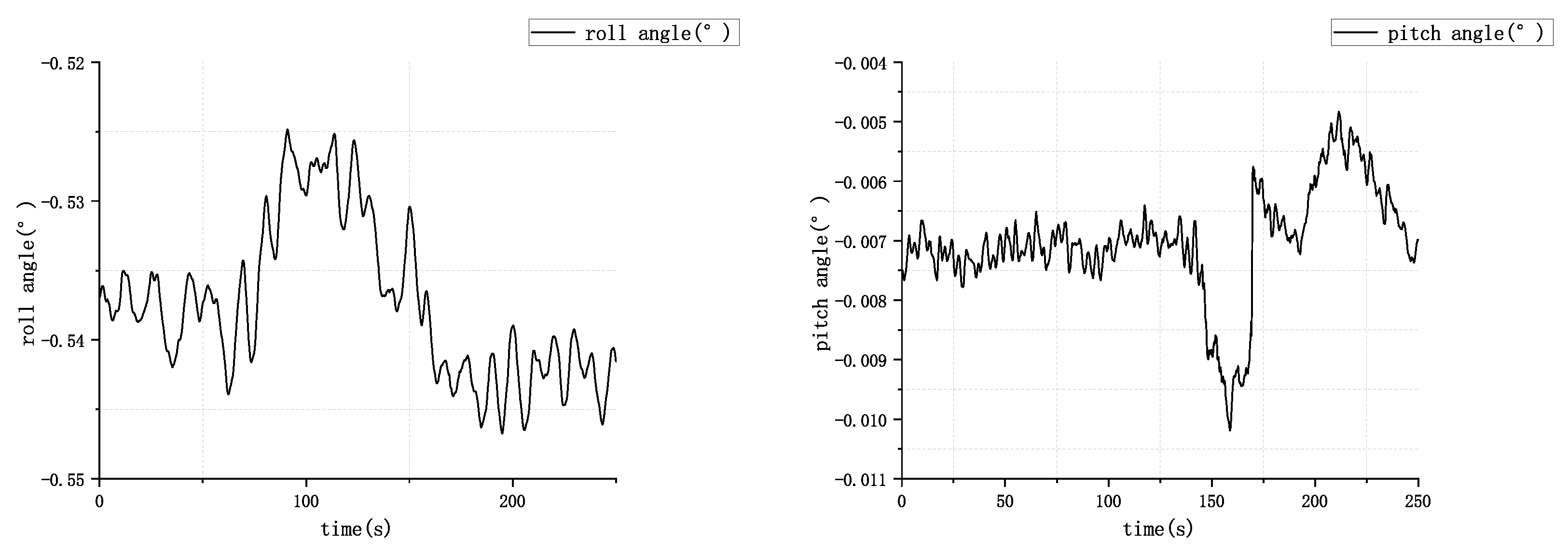
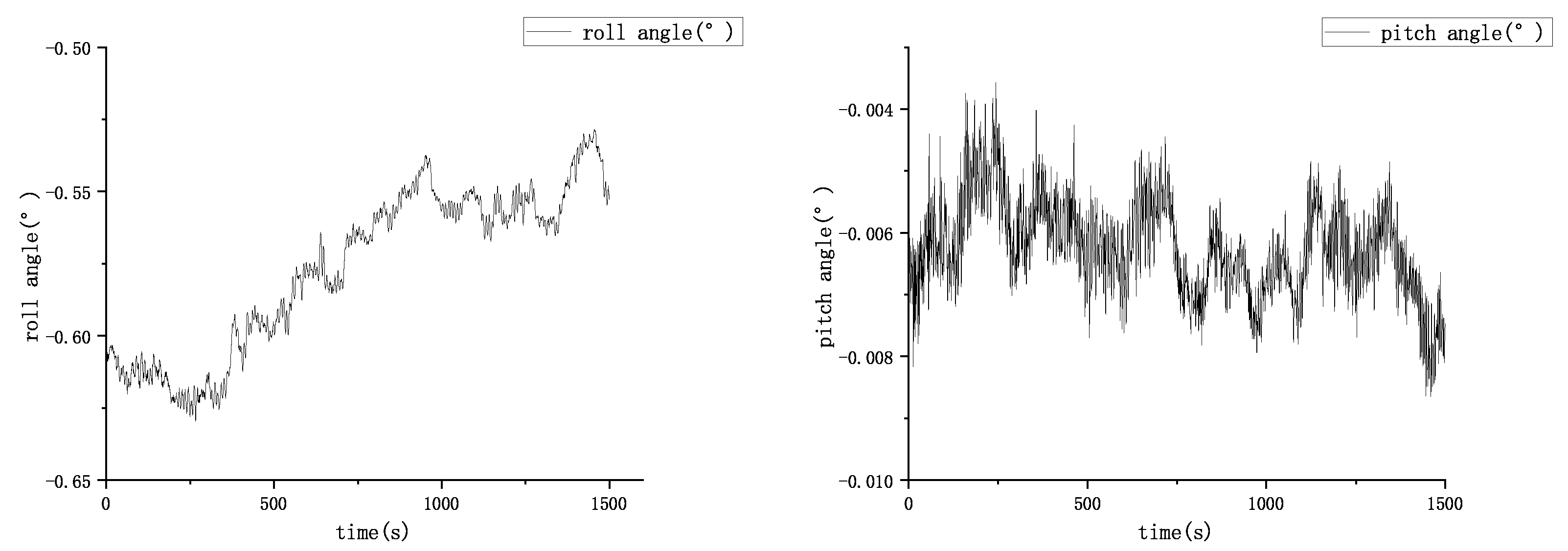
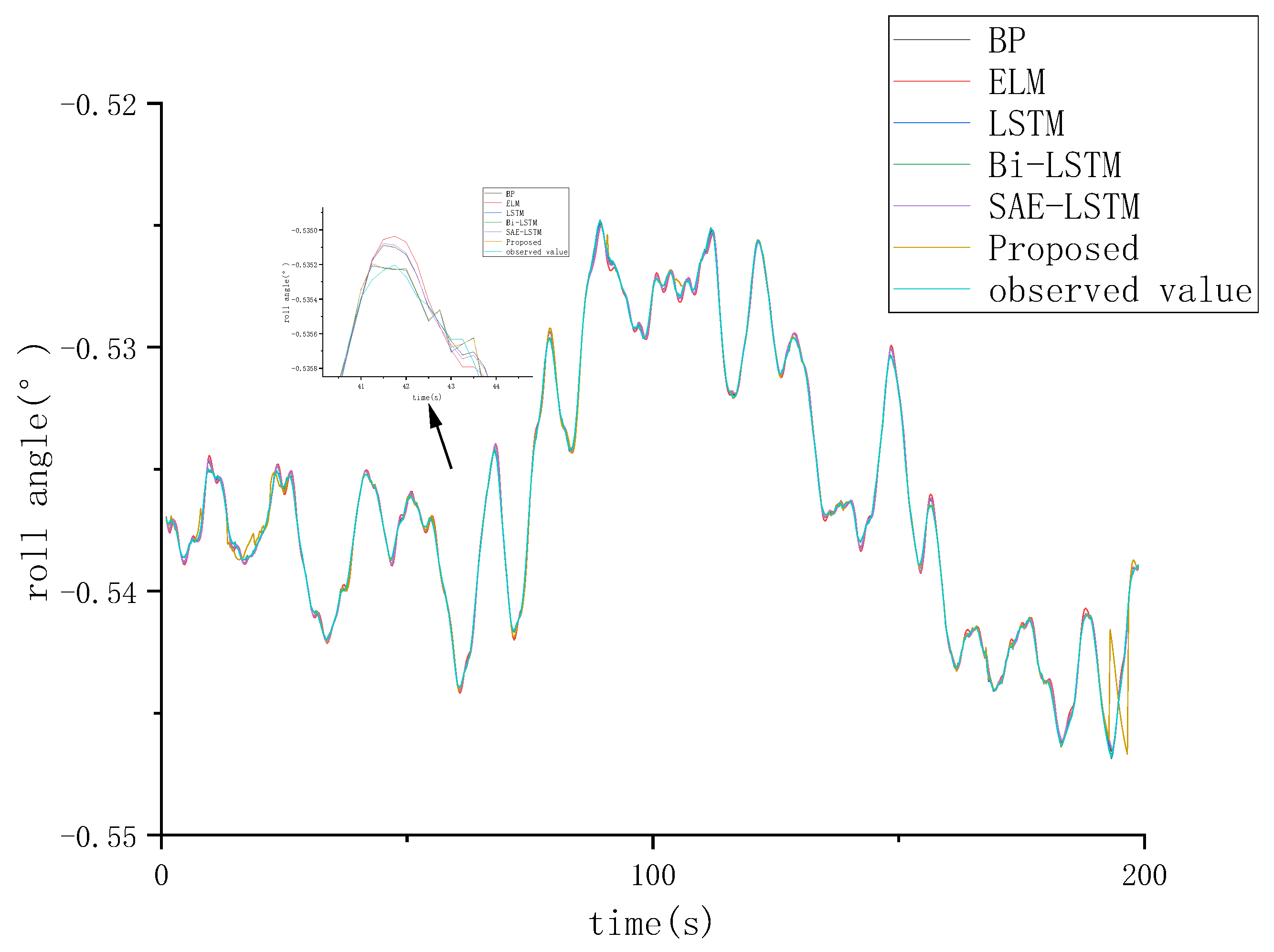
4.3. Roll Angle Prediction Results and Analysis

To ensure the fairness of the experiment, the initial parameters are set to remain the same, and the detailed model parameter settings are listed in Table 3. In order to prove the effectiveness of the hybrid prediction model proposed in this paper, adaptive PSO–LSTM and EMD–LSTM were selected as comparison models. Additionally, the BP neural network, ELM, LSTM, and its variant neural networks were selected to prove the effectiveness in short-term ship motion attitude prediction.
Taking Dataset 1 as an example, different benchmark models of roll angle prediction are shown in Figure 12 and Figure 13. It is obvious that LSTM and its variant neural networks have better performance compared with the BP neural network and ELM, which proves the superiority of the deep learning method and that the LSTM neural network has higher accuracy. The errors between the predicted values and the recorded values for each method are shown in Figure 14 and Figure 15. Additionally, the statistical results of errors in Dataset 1 are shown in Table 4, where LSTM, EMD–LSTM, and the adaptive PSO–LSTM method were selected to make comparisons with the proposed method to prove that EMD and adaptive PSO improved the LSTM neural network and had better adaptability. Although the input of the dataset is changed, the network structure can also be changed at the same time to achieve the best prediction performance. However, the above results are for one-step predictions. In practical engineering applications, short-term prediction of ship motion attitude generally requires multi-step-ahead predictions. This result means the prediction error ahead of different steps is based on the former observed value and current prediction value and has error accumulation, which is inevitable.
In this paper, one-step, two-step, and three-step-ahead predictions were set aiming at all the datasets. The roll angle prediction errors of different models are shown in Table 5. As for dataset 1, ELM and the proposed method indicate the obvious error accumulation phenomenon, and the error result shows that almost all the datasets using the selected methods showed error accumulation as the number of predicted steps increases. Theoretically speaking, error accumulation is inevitable, but in practical prediction, not all neural networks demonstrate such situations, especially when using different datasets.
Figure 16 and Figure 17 show the error distribution of one-step-ahead, two-step-ahead, and three-step-ahead predictions with different models in a more visual way. The ELM method and BP neural network had a higher error in the three-step-ahead prediction, which may be due to the simple network structures.

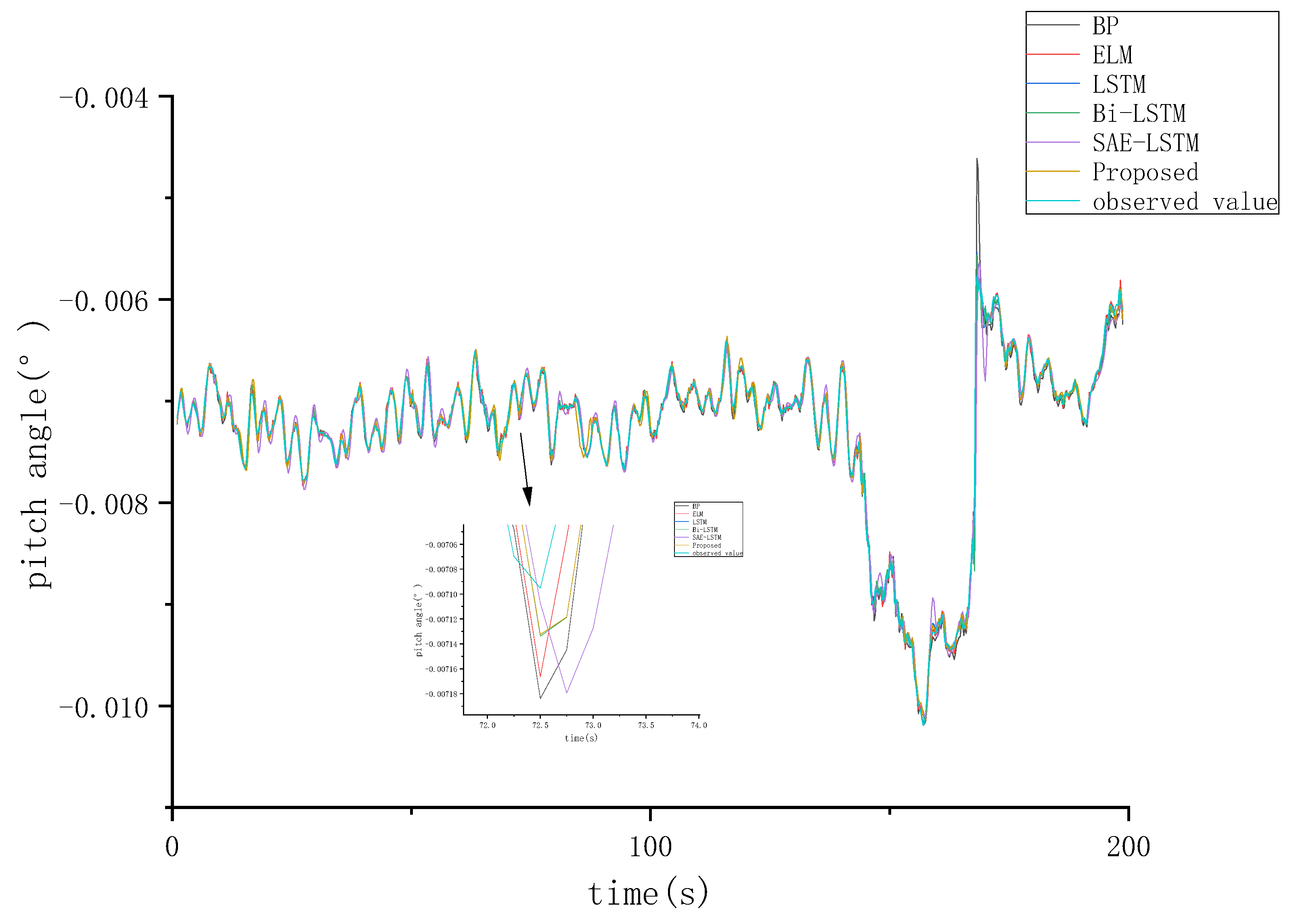
4.4. Pitching Angle Prediction Results and Analysis

Taking Dataset 1 as an example, different benchmark models for pitching angle prediction results are shown in Figure 18 and Figure 19. Figure 18 indicates prediction results in 200 s, and Figure 19 shows the testing data in 50 s. It can be seen that LSTM and BiLSTM had better fitting performance. In order to prove that EMD and adaptive PSO are both effective methods in improving LSTM for short-term ship attitude prediction, EMD–LSTM and adaptive PSO–LSTM were chosen for comparison, and the statistical results of errors are shown in Table 6. As a whole, adaptive PSO–LSTM had lower MAE and RMSE compared with EMD–LSTM, which means that adaptive PSO improves adaptability by adjusting network parameters dynamically and has more accurate results. Although the MAPE result is different from the MAE and RMSE results, the two method prediction results are similar and can be ignored. EMD is mainly used to reduce the nonstationary characteristic before dividing fixed window length time series data into training and testing datasets. The proposed model had the lowest error results and can further prove the validity of short-term prediction. The error results between the prediction and the recorded values for each method are shown in Figure 20 and Figure 21. Similar to roll angle prediction experiments, pitching angle prediction of all the datasets is shown in Table 7, which shows that the proposed model outperforms the other methods in terms of one-step-ahead, two-step-ahead, and three-step-ahead prediction with the lowest error results. Still, the error accumulation is obvious.
Both Figure 22 and Figure 23 show the error distribution of the one-step-ahead, two-step-ahead, and three-step-ahead predictions of pitching angle with different models in a more visual way, and MAPE distribution shows an increasing trend. Compared with the previous model, the BP neural network still had the higher error results in multi-step-ahead predictions. It is worth noting that the SAELSTM method also had poor prediction performance, which demonstrates that complex networks do not always result in better predictions. On the contrary, this may cause a long overall prediction time.

5. Conclusions

To improve the predicted performance of roll and pitch angles in the short term, a novel hybrid EMD-adaptive PSO–LSTM model with the sliding window approach was proposed in this paper. Firstly, in order to solve the problem of nonlinear and nonstationary data affecting the prediction accuracy, an EMD-based denoising method was proposed to smooth the original ship motion time series data. Secondly, an adaptive PSO algorithm was proposed to optimize the number of hidden units in the LSTM neural network to improve the accuracy of ship motion attitude prediction. To properly evaluate the performance of the proposed model, five sets of sea trial data were used for verification. The experimental results show the superiority of the proposed algorithm.

Author Contributions

X.G.; Conceptualization, methodology, software, writing—original draft, Y.L.; supervision, formal analysis, mathematical check, writing—review and editing, Q.S. All authors have read and agreed to the published version of the manuscript.

Funding

This work is supported by the Foundation of National Defense Key Laboratory(2021-JCJQ-LB-066-12), National Natural Science Foundation of China (No.52271311), Heilongjiang Touyan Innovation Team Program.

Institutional Review Board Statement

Not applicable.

Informed Consent Statement

Not applicable.

Data Availability Statement

The data presented in this study are available on request from the corresponding author due to privacy restrictions.

Conflicts of Interest

The authors declare no conflict of interest.

References

  1. Tang, G.; Wu, Y.; Li, C.; Wong, P.K.; Xiao, Z.; An, X. A novel wind speed interval prediction based on error prediction method. IEEE Trans. Ind. Inform. 2020, 16, 6806–6815. [Google Scholar] [CrossRef]
  2. Ali, M.; Prasad, R. Significant wave height forecasting via an extreme learning machine model integrated with improved complete ensemble empirical mode decomposition. Renew. Sustain. Energy Rev. 2019, 104, 281–295. [Google Scholar] [CrossRef]
  3. Wang, Z.; Zou, Z.; Soares, C.G. Identification of ship manoeuvring motion based on nu-support vector machine. Ocean Eng. 2019, 183, 270–281. [Google Scholar] [CrossRef]
  4. Wei, W.W.S. Time series analysis. In The Oxford Handbook of Quantitative Methods in Psychology; Oxford Library: Oxford, UK, 2006; Volume 2. [Google Scholar]
  5. Majnarić, D.; Šegota, S.B.; Lorencin, I.; Car, Z. Prediction of main particulars of container ships using artificial intelligence algorithms. Ocean Eng. 2022, 265, 112571. [Google Scholar] [CrossRef]
  6. Kumari, P.; Toshniwal, D. Long short term memory–Convolutional neural network based deep hybrid approach for solar irradiance forecasting. Appl. Energy 2021, 295, 117061. [Google Scholar] [CrossRef]
  7. Sarıca, B.; Eğrioxgxlu, E.; Barış, A. A new hybrid method for time series forecasting: Ar–anfis. Neural Comput. Appl. 2018, 29, 749–760. [Google Scholar] [CrossRef]
  8. Khan, A.; Bil, C.; Marion, K.E. Ship motion prediction for launch and recovery of air vehicles. In Proceedings of the OCEANS 2005 MTS/IEEE, Washington, DC, USA, 17–23 September 2005; pp. 2795–2801. [Google Scholar]
  9. Kaplan, P. A study of prediction techniques for aircraft carrier motions at sea. J. Hydronautics 1969, 3, 121–131. [Google Scholar] [CrossRef]
  10. Fossen, T.I.; Perez, T. Kalman filtering for positioning and heading control of ships and offshore rigs. Control. Syst. IEEE 2009, 29, 32–46. [Google Scholar]
  11. Wang, W.; Chau, K.; Xu, D.; Chen, X. Improving forecasting accuracy of annual runoff time series using arima based on eemd decomposition. Water Resour. Manag. 2015, 29, 2655–2675. [Google Scholar] [CrossRef]
  12. ElMoaqet, H.; Tilbury, D.M.; Ramachandran, S.K. Ramachandran. Multi-step ahead predictions for critical levels in physiological time series. IEEE Trans. Cybern. 2016, 46, 1704–1714. [Google Scholar] [CrossRef]
  13. Liu, X.M.; Zhang, Y.Y.; Feng, X.Y.; Wang, Q.X. A novel method for hull’s three dimensional deformation measurement. Appl. Mech. Mater. Trans. Technol. Publ. 2013, 344, 93–98. [Google Scholar] [CrossRef]
  14. Xu, D.; Wang, Y.; Peng, P.; Beilun, S.; Deng, Z.; Guo, H. Real-time road traffic state prediction based on kernel-knn. Transportmetrica 2020, 16, 104–118. [Google Scholar] [CrossRef]
  15. Xiao, X.; Duan, H.; Wen, J. A novel car-following inertia grey model and its application in forecasting short-term traffic flow. Appl. Math.l Modell. 2020, 87, 546–570. [Google Scholar] [CrossRef]
  16. Yang, Y.; Tu, H.; Song, L.; Chen, L.; Xie, D.; Sun, J. Research on accurate prediction of the container ship resistance by rbfnn and other machine learning algorithms. J. Mar. Sci. Eng. 2021, 9, 376. [Google Scholar] [CrossRef]
  17. Sun, Q.; Tian, Y.; Diao, M. Cooperative localization algorithm based on hybrid topology architecture for multiple mobile robot system. IEEE Internet Things J. 2018, 2018, 1. [Google Scholar] [CrossRef]
  18. Sun, Q.; Tang, Z.; Gao, J.; Zhang, G. Short-term ship motion attitude prediction based on lstm and gpr. Appl. Ocean Res. 2022, 118, 118. [Google Scholar] [CrossRef]
  19. Ye, F.; Chen, J.; Tian, Y.; Jiang, T. Cooperative multiple task assignment of heterogeneous uavs using a modified genetic algorithm with multi-type-gene chromosome encoding strategy. J. Intell. Robot. Syst. 2020, 100, 1–13. [Google Scholar] [CrossRef]
  20. Babu, C.N.; Reddy, B.E. A moving-average filter based hybrid arima–ann model for forecasting time series data. Appl. Soft Comput. 2014, 23, 27–38. [Google Scholar] [CrossRef]
  21. Moreira, L.; Soares, C.G. Simulating ship manoeuvrability with artificial neural networks trained by a short noisy data set. J. Mar. Sci. Eng. 2023, 11, 1. [Google Scholar] [CrossRef]
  22. Li, J.; Dai, Q.; Ye, R. A novel double incremental learning algorithm for time series prediction. Neural Comput. Appl. 2019, 31, 6055–6077. [Google Scholar] [CrossRef]
  23. Dai, X.; Sheng, K.; Shu, F. Ship power load forecasting based on pso-svm. Math. Biosci. Eng. 2022, 19, 4547–4567. [Google Scholar] [CrossRef] [PubMed]
  24. Saha, A.; Basu, S.; Datta, A. Random forests for spatially dependent data. J. Am. Stat. Assoc. 2021, 1–19. [Google Scholar] [CrossRef]
  25. Liu, H.; Tian, H.; Chen, C.; Li, Y. An experimental investigation of two wavelet-mlp hybrid frameworks for wind speed prediction using ga and pso optimization. Int. J. Electr. Power Energy Syst. 2013, 52, 161–173. [Google Scholar] [CrossRef]
  26. Atiquzzaman, M.; Kandasamy, J. Robustness of extreme learning machine in the prediction of hydrological flow series. Comput. Geosci. 2018, 120, 105–114. [Google Scholar] [CrossRef]
  27. Wang, H.; Liu, X.; Song, P.; Tu, X. Sensitive time series prediction using extreme learning machine. Int. J. Mach. Learn. Cybern. 2019, 10, 3371–3386. [Google Scholar] [CrossRef]
  28. Huang, G.; Zhu, Q.; Siew, C. Extreme learning machine: Theory and applications. Neurocomputing 2006, 70, 489–501. [Google Scholar] [CrossRef]
  29. Mahdi, K.; Wang, J. Spatio-temporal graph deep neural network for short-term wind speed forecasting. IEEE Trans. Sustain. Energy 2018, 2, 1. [Google Scholar]
  30. Qin, S.-Q.; De, J.; Wu, W. A hybrid ar-dwt-emd model for the short-term prediction of nonlinear and nonstationary ship motion. In Proceedings of the IEEE 2016 Chinese Control and Decision Conference (CCDC), Yinchuan, China, 28–30 May 2016; pp. 4042–4047. [Google Scholar]
  31. Veltcheva, A.; Soares, C.G. Analysis of wave-induced vertical ship responses by hilbert-huang transform method. Ocean Eng. 2023, 269, 113533. [Google Scholar] [CrossRef]
  32. Wang, Y.; Wang, H.; Zou, D.; Fu, H. Ship roll prediction algorithm based on bi-lstm-tpa combined model. J. Mar. Sci. Eng. 2021, 9, 387. [Google Scholar] [CrossRef]
  33. El Said, A.; El Jamiy, F.; Higgins, J.; Wild, B.; Desell, T. Optimizing long short-term memory recurrent neural networks using ant colony optimization to predict turbine engine vibration. Appl. Soft Comput. 2018, 73, 969–991. [Google Scholar] [CrossRef] [Green Version]
  34. Peng, X.; Zhang, B.; Zhou, H. An improved particle swarm optimization algorithm applied to long short-term memory neural network for ship motion attitude prediction. Trans. Inst. Meas. Control. 2019, 41, 4462–4471. [Google Scholar] [CrossRef]
  35. Qian, L.; Wang, W.; Chen, G.; Yu, M. A fetal electrocardiogram signal extraction method based on long short term memory network optimized by genetic algorithm. J. Biomed. Eng. 2021, 38, 257–267. [Google Scholar]
  36. Yin, J.; Wang, N.; Perakis, A.N. A real-time sequential ship roll prediction scheme based on adaptive sliding data window. IEEE Trans. Syst. Man Cybern. Syst. 2017, 48, 2115–2125. [Google Scholar] [CrossRef]
  37. Yao, Y.; Han, L.; Wang, J. Lstm-pso: Long short-term memory ship motion prediction based on particle swarm optimization. In Proceedings of the 2018 IEEE CSAA Guidance, Navigation and Control Conference (CGNCC), Xiamen, China, 10–12 August 2018; pp. 1–5. [Google Scholar]
  38. Nie, Z.; Yuan, Y.; Xu, D.; Shen, F. Research on support vector regression model based on different kernels for short-term prediction of ship motion. In Proceedings of the IEEE 2019 12th International Symposium on Computational Intelligence and Design (ISCID), Hangzhou, China, 14–15 December 2019; Volume 1, pp. 61–64. [Google Scholar]
  39. Zhang, Z.; Yin, J.; Hu, J.; Liu, C. Ship rolling motion prediction and analysis based on grey pso-anfis model. Sci. Technol. Eng. 2016, 16, 124–129. [Google Scholar]
  40. Hochreiter, S.; Schmidhuber, J. Long short-term memory. Neural Comput. 1997, 9, 1735–1780. [Google Scholar] [CrossRef] [PubMed]
Figure 1. Sliding window approach for multi-step.
Jmse 11 00466 g001
Figure 2. LSTM cell structure.
Jmse 11 00466 g002
Figure 3. The flowchart of adaptive PSO–LSTM prediction method.
Jmse 11 00466 g003
Figure 4. The overall structure of the proposed hybrid prediction model.
Jmse 11 00466 g004
Figure 5. The scene of raw data acquisition.
Jmse 11 00466 g005
Figure 6. Dataset 1: The raw roll and pitch angle of the ship.
Jmse 11 00466 g006
Figure 7. Dataset 2: The raw roll and pitch angle of the ship.
Jmse 11 00466 g007
Figure 8. Dataset 3: The raw roll and pitch angle of the ship.
Jmse 11 00466 g008
Figure 9. Dataset 4: The raw roll and pitch angle of the ship.
Jmse 11 00466 g009
Figure 10. Dataset 5: The raw roll and pitch angle of the ship.
Jmse 11 00466 g010
Figure 11. Optimization iteration results of different test functions: (a) Rosenbrock test function; (b) Griewank test function.
Jmse 11 00466 g011
Figure 12. Roll angle prediction results in the training set of Dataset 1.
Jmse 11 00466 g012
Figure 13. Roll angle prediction results in the testing set of Dataset 1.
Jmse 11 00466 g013
Figure 14. Roll angle prediction error results in the training set of Dataset 1.
Jmse 11 00466 g014
Figure 15. Roll angle prediction error results in the testing set of Dataset 1.
Jmse 11 00466 g015
Figure 16. Roll angle prediction error distribution of Dataset 1.
Jmse 11 00466 g016
Figure 17. Roll angle prediction error distribution of Dataset 2.
Jmse 11 00466 g017
Figure 18. Pitch angle prediction results in the training set of Dataset 1.
Jmse 11 00466 g018
Figure 19. Pitch angle prediction results in the testing set of Dataset 1.
Jmse 11 00466 g019
Figure 20. Pitch angle prediction error results in the training set of Dataset 1.
Jmse 11 00466 g020
Figure 21. Pitch angle prediction error results in the testing set of Dataset 1.
Jmse 11 00466 g021
Figure 22. Pitch angle prediction error distribution of Dataset 1.
Jmse 11 00466 g022
Figure 23. Pitch angle prediction error distribution of Dataset 2.
Jmse 11 00466 g023
Table 1. The description of different raw datasets.
DatasetThe Start Time of Record DataDuration (s)Roll Angle (°)Pitch Angle (°)
Average ValueMaximum ValueMinimum ValueAverage ValueMaximum ValueMinimum Value
#120 December 2014 12:10:21.000250−0.543618911−0.530798−0.553233−0.00710956−0.004698−0.010346
#220 December 2014 16:30:59:000250−0.560047567−0.543898−0.579896−0.006100966−0.004592−0.007791
#320 December 2014 12:30:00:0001500−0.621413551−0.534555−0.636779−0.006321536−0.003541−0.00883
#411 March 2015 12:48:22:2503000.7299846178.2649−6.5716−0.047186850.8845−0.9738
#519 April 2016 16:12:56:0273000.4378979831.6867−1.2942−0.738008183−0.3692−1.1086
Table 2. Test functions to test the performance of the adaptive PSO algorithm.
NameTest Function Expression
Rosenbrock f ( x , y ) = ( 1 x ) 2 + 100 ( y x 2 ) 2
Griewank f ( x i ) = i = 1 N x i 2 4000 i = 1 N cos x i i + 1
Table 3. Settings of different model parameters.
ModelParametersValues
BPNumber of Hidden Neurons10
ELMTransfer Functionsine function
Number of Hidden Neurons10
LSTMHidden Units10
MaxEpochs250
Initial learning rate0.01
numFeatures1
numResponse1
droprate0.2
activation functionsigmoid, tanh
MiniBatchSize128
OptimizerAdam
Bi-LSTMNumber of Hidden Neurons10
Activation functionsigmoid, tanh
SAE-LSTMSparsityProportion0.6
Number of Hidden Neurons10
ProposedEMD decomposition7Imfs + res.(take roll angle in dataset1 as an example)
Sliding window length10
LSTM layerthe same as LSTM model
Table 4. Statistical results of roll angle prediction errors in Dataset 1.
MethodMAE ( × 10 5 )MAPE ( × 10 6 )RMSE ( × 10 5 )
LSTM2.856.424.63
adaptive PSO–LSTM2.514.602.79
EMD–LSTM2.745.003.06
proposed1.402.601.62
Table 5. The roll angle prediction errors of different models.
DatasetModelRMSE ( × 10 5 )MAE ( × 10 5 )MAPE ( × 10 5 )
1 Step2 Steps3 Steps1 Step2 Steps3 Steps1 Step2 Steps3 Steps
#1BP13.986510.950417.712011.41208.120114.23600.10630.07680.1345
ELM21.959630.667632.062017.787624.430325.53100.16570.23110.2414
LSTM6.56316.56196.82075.22095.21045.52770.04860.04920.0522
Bi-LSTM6.880518.90877.80665.489115.23016.03380.05110.14410.0570
SAE-LSTM16.209715.430717.726012.957912.568514.37100.12080.11890.1360
Proposed1.62002.25002.89301.40003.85203.90500.02620.02540.0295
#2BP24.184124.600128.341018.072719.955023.51700.16350.18310.4260
ELM21.053442.206577.090227.066433.935846.41720.170.31100.0753
LSTM24.053324.160415.708014.845217.394418.21500.13460.15730.2160
Bi-LSTM22.556325.763329.26615.917817.095122.9810.1440.15970.2109
SAE-LSTM55.675926.950144.321818.766521.560035.36440.16380.19790.3240
Proposed15.521118.42619.725613.254214.981217.31580.028450.032490.03674
#3BP16.257416.511217.21547.83798.43299.12451.92802.62202.6270
ELM15.311316.254818.75128.17298.21468.75121.92203.51403.2140
LSTM8.37129.21409.74516.15356.84217.15000.10060.19200.5320
Bi-LSTM11.318012.054112.95426.16786.98747.54130.12300.36100.6210
SAE-LSTM18.705119.012421.02446.61677.15938.17360.18300.62700.8240
Proposed6.24517.62149.02155.21545.92416.83140.09800.16700.3450
#4BP55.125055.812556.012421.215422.437523.45712.98533.04273.6125
ELM50.512051.032151.874223.645123.946124.65182.41272.46722.6523
LSTM37.012037.620038.312415.224316.021416.95721.12451.24511.3526
Bi-LSTM40.152042.015842.654716.275116.954217.95121.42671.51341.5142
SAE-LSTM47.042048.321947.012416.958517.956118.64121.34211.40001.4873
Proposed25.045026.012727.654114.321414.954615.31250.87130.89711.0821
#5BP51.01752.427552.978122.812423.124523.99712.64522.94513.8451
ELM50.42351.437953.124521.464822.987523.78152.12522.32152.4025
LSTM38.04238.451239.412417.514517.451618.91551.46521.48241.6715
Bi-LSTM42.02442.372143.751217.689117.981518.67851.34251.65411.7512
SAE-LSTM43.12744.128945.012418.751218.791219.15440.98421.02451.6522
Proposed32.04532.781833.158715.421515.975416.32420.94211.01341.6452
Table 6. Statistical results of pitch angle prediction errors in Dataset 1.
MethodMAE ( × 10 5 )MAPE ( × 10 5 )RMSE ( × 10 5 )
LSTM2.361.543.76
adaptive PSO–LSTM0.590.810.76
EMD–LSTM1.440.201.82
proposed0.3660.490.46
Table 7. The pitch angle prediction errors of different models.
DatasetModelRMSE ( × 10 4 )MAE ( × 10 4 )MAPE ( × 10 4 )
1 Step2 Steps3 Steps1 Step2 Steps3 Steps1 Step2 Steps3 Steps
#1BP2.48802.31173.16141.93401.83542.42251.47791.44341.8784
ELM2.39141.07851.20831.42250.75630.86801.09490.60070.6957
LSTM1.29501.70181.70270.98891.30261.30120.76231.01371.0121
Bi-LSTM1.10731.51011.42170.84231.15471.07810.65270.90160.8431
SAE-LSTM2.06352.07842.39061.58001.60441.85531.22901.24871.4431
Proposed1.02051.54262.43520.75020.96420.98520.70520.85430.9548
#2BP0.49260.50040.50210.39160.3960.39700.32990.33940.3409
ELM0.49860.52850.52950.39670.41530.42100.33420.35510.3604
LSTM0.40790.42240.43210.34740.32720.33460.27970.28610.2932
Bi-LSTM0.44780.45010.45210.35950.36440.36380.30430.31280.3118
SAE-LSTM0.85500.77290.8690.72170.69850.61430.52070.60020.6103
Proposed0.30520.35640.42150.30250.33450.35010.20150.23410.2654
#3BP3.12473.45214.04212.32102.39542.95251.64211.75121.7834
ELM3.45413.64223.98752.04232.32122.62151.04551.42451.4625
LSTM2.31242.42152.51241.04251.32511.42360.64210.66780.8451
Bi-LSTM2.64522.78122.98151.34511.36421.42030.84510.89450.9451
SAE-LSTM2.42152.64512.98751.62541.63551.85330.83420.86430.8965
Proposed1.45211.67511.72350.93451.04211.34250.64210.65120.7345
#4BP7.15157.64218.45124.04514.31254.54212.64252.75622.7865
ELM7.12457.52457.61543.45123.64273.98542.45142.64522.7635
LSTM4.45124.64575.04212.45122.56342.87541.45161.46341.6552
Bi-LSTM4.61244.78154.98712.94513.01243.01251.64211.75421.7954
SAE-LSTM5.15445.34255.21542.87542.98453.01241.67841.97802.0451
Proposed3.24513.64523.98751.94582.01432.13451.34511.36491.4535
#5BP7.91468.12468.95784.04144.32154.94852.58612.67842.7625
ELM7.81248.04518.65244.61524.97815.01452.54632.64582.8451
LSTM5.64125.72155.98413.01543.46143.84521.65351.68541.7058
Bi-LSTM5.98426.24516.37583.12453.24813.45851.67841.65241.7815
SAE-LSTM6.51677.01247.62553.46253.64214.04581.67361.75441.8065
Proposed4.56714.68754.95872.84512.98453.01421.16431.42681.3815
Disclaimer/Publisher’s Note: The statements, opinions and data contained in all publications are solely those of the individual author(s) and contributor(s) and not of MDPI and/or the editor(s). MDPI and/or the editor(s) disclaim responsibility for any injury to people or property resulting from any ideas, methods, instructions or products referred to in the content.

