
Southern South China Sea Dynamics: Sea Level Change from Coupled Model Intercomparison Project Phase 6 (CMIP6) in the 21st Century
 , , , , , ,
Abstract
:1. Introduction
2. Materials and Methods
3. Results
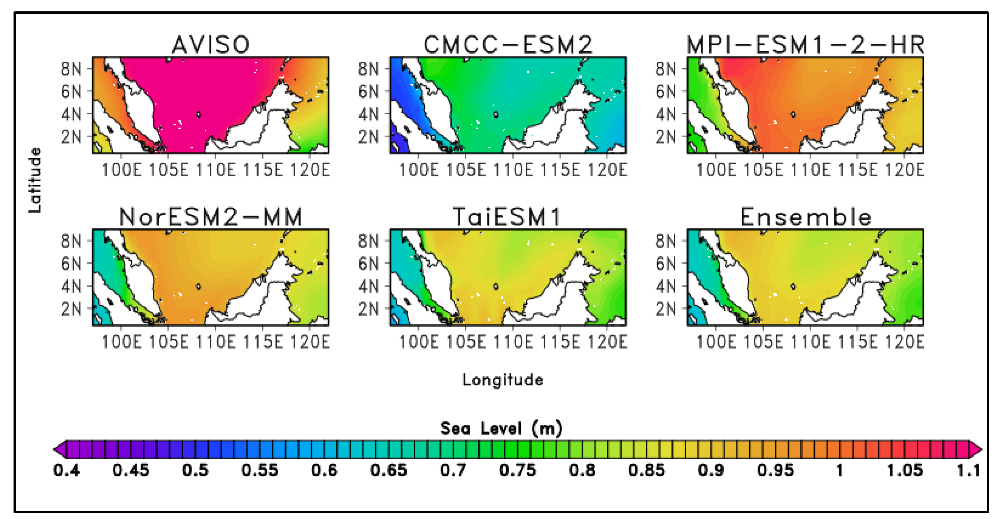
3.1. Historical Spatial Analysis of Sea Levels around Malaysia
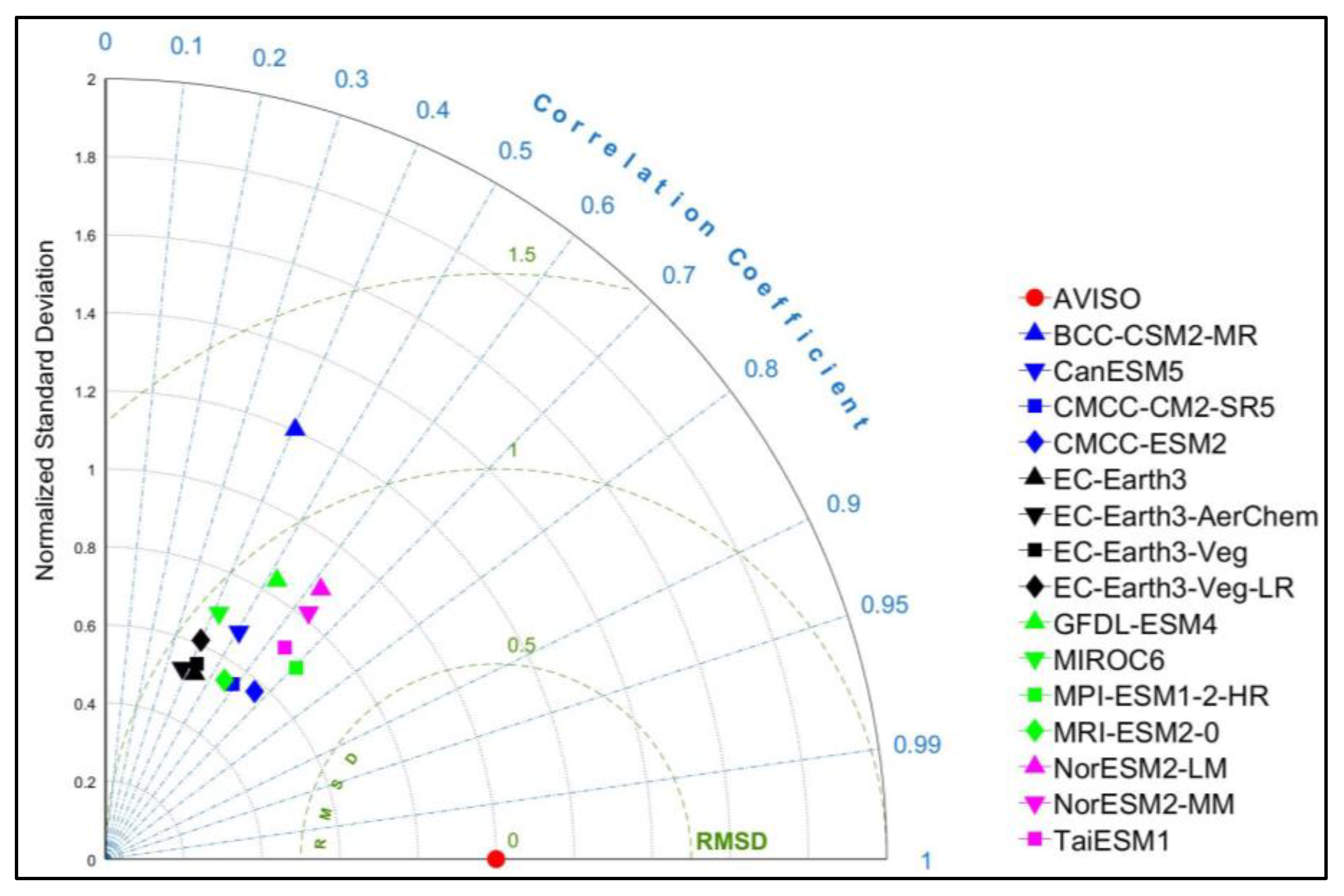
3.2. Selection of Models Based on Spatial Analysis
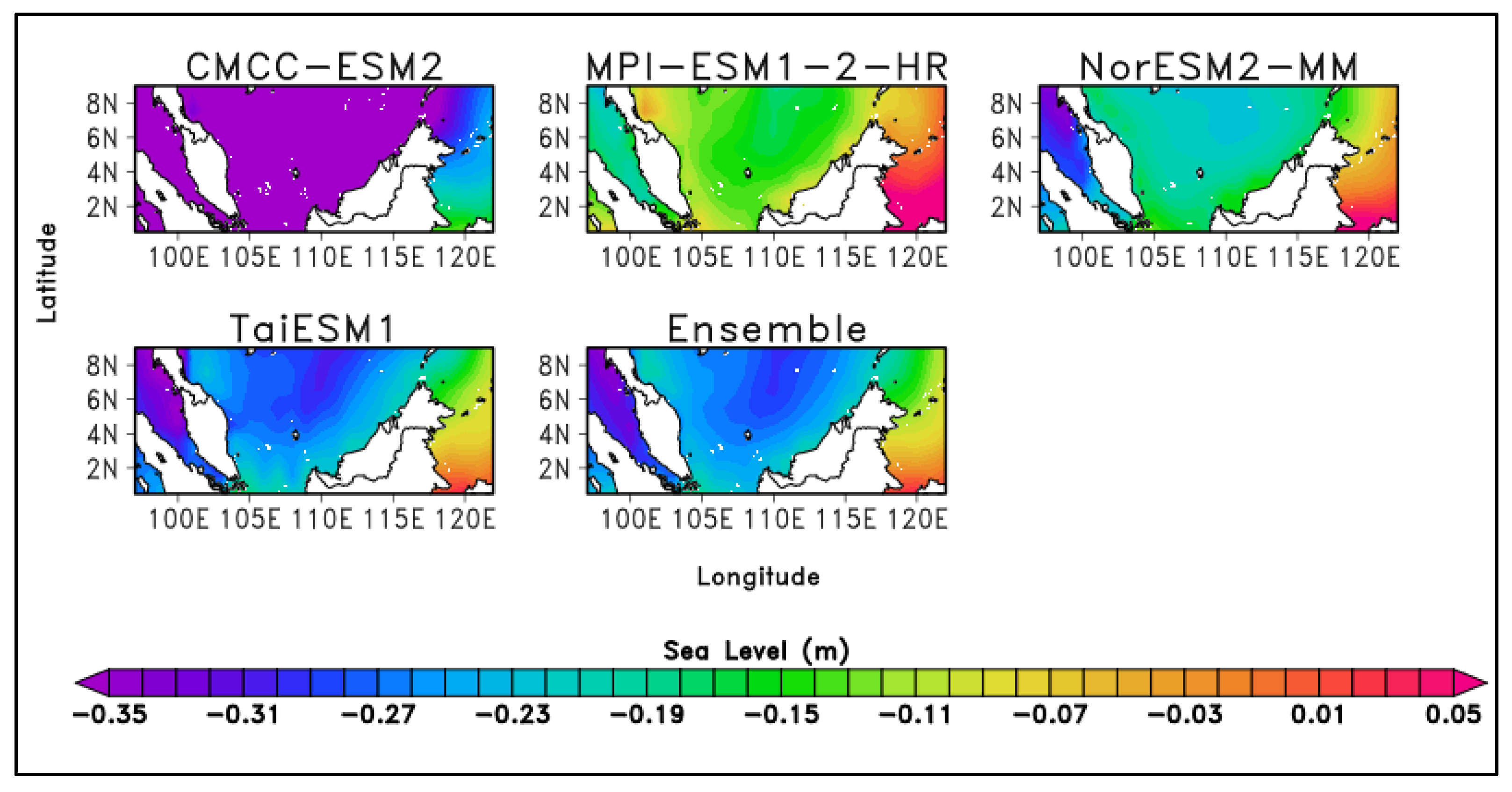
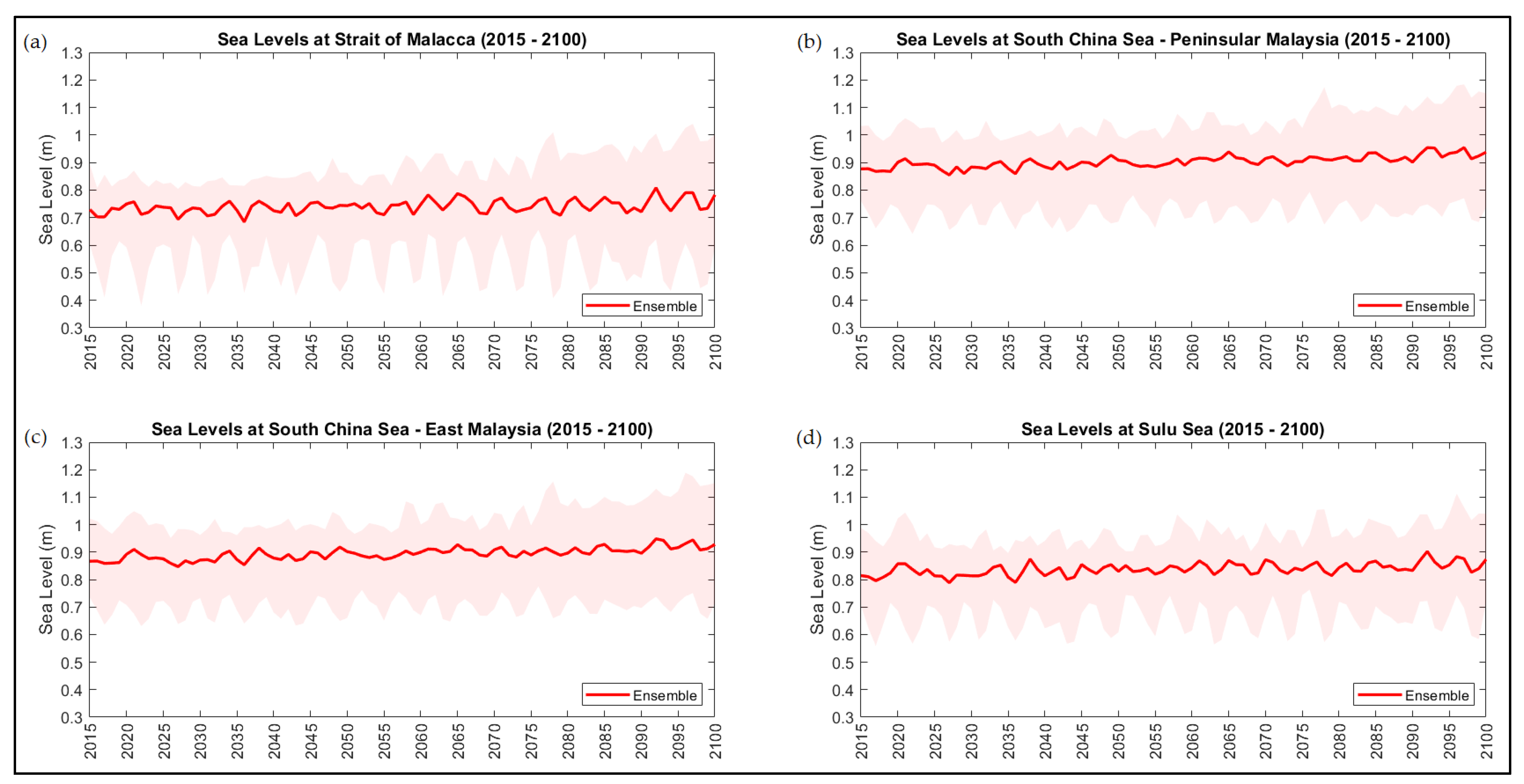
3.3. Sea Level Projection for Malaysian Seas
4. Discussion
Sea Level Projection for Malaysian Seas
5. Conclusions
Author Contributions
Funding
Institutional Review Board Statement
Informed Consent Statement
Data Availability Statement
Acknowledgments
Conflicts of Interest
References
- Chen, D.; Rojas, M.; Samset, B.H.; Cobb, K.; Diongue Niang, A.; Edwards, P.; Emori, S.; Faria, S.H.; Hawkins, E.; Hope, P.; et al. Framing, Context, and Methods. In Climate Change 2021: The Physical Science Basis. Contribution of Working Group I to the Sixth Assessment Report of the Intergovernmental Panel on Climate Change; Masson-Delmotte, V., Zhai, P., Pirani, A., Connors, S.L., Péan, C., Berger, S., Caud, N., Chen, Y., Goldfarb, L., Gomis, M.I., Eds.; Cambridge University Press: Cambridge, UK, 2021; pp. 147–286. [Google Scholar] [CrossRef]
- Sarkar, M.; Kabir, S.; Begum, R.A.; Pereira, J.J.; Jaafar, A.H.; Saari, M.Y. Impacts of and adaptations to sea level rise in Malaysia. Asian J. Water Environ. Pollut. 2014, 11, 29–36. [Google Scholar]
- Nicholls, R.J.; Cazenave, A. Sea-level rise and its impact on coastal zones. Science 2010, 328, 1517–1520. [Google Scholar] [CrossRef] [PubMed]
- Warrick, R.A.; Warrick, R.A.; Barrow, E.M.; Wigley, T.M.L. Climate and Sea Level Change: Observations, Projections and Implications; Cambridge University Press: Cambridge, UK, 1993. [Google Scholar]
- Milliman, J.D.; Broadus, J.M.; Gable, F. Environmental and economic implications of rising sea level and subsiding deltas: The Nile and Bengal examples. Ambio 1989, 18, 340–345. [Google Scholar]
- Barth, M.C.; Titus, J.G. Greenhouse Effect and Sea Level Rise: A Challenge for This Generation; Van Nostrand Reinhold: New York, NY, USA, 1984; p. 325. [Google Scholar]
- Sung, H.M.; Kim, J.; Lee, J.H.; Shim, S.; Boo, K.O.; Ha, J.C.; Kim, Y.H. Future changes in the global and regional sea level rise and sea surface temperature based on cmip6 models. Atmosphere 2021, 12, 90. [Google Scholar] [CrossRef]
- Grinsted, A.; Jevrejeva, S.; Riva, R.E.M.; Dahl-Jensen, D. Sea level rise projections for northern Europe under RCP8. 5. Clim. Res. 2015, 64, 15–23. [Google Scholar] [CrossRef] [Green Version]
- Christensen, J.H.; Hewitson, B.; Busuioc, A.; Chen, A.; Gao, X.; Held, I.; Jones, R.; Kolli, R.K.; Kwon, W.-T.; Laprise, R.; et al. Regional Climate Projections 2007, Chapter 11. Available online: https://www.ipcc.ch/site/assets/uploads/2018/02/ar4-wg1-chapter11-1.pdf (accessed on 7 April 2022).
- Jennath, A.; Krishnan, A.; Paul, S.K.; Bhaskaran, P.K. Climate projections of sea level rise and associated coastal inundation in atoll islands: Case of Lakshadweep Islands in the Arabian Sea. Reg. Stud. Mar. Sci. 2021, 44, 101793. [Google Scholar] [CrossRef]
- Ghazali, N.H.M. Coastal erosion and reclamation in Malaysia. Aquat. Ecosyst. Health Manag. 2006, 9, 237–247. [Google Scholar] [CrossRef]
- Ehsan, S.; Begum, R.A.; Nor, N.G.M.; Maulud, K.N.A. Current and potential impacts of sea level rise in the coastal areas of Malaysia. IOP Conf. Ser. Earth Environ. Sci. 2019, 228, 12023. [Google Scholar] [CrossRef]
- Nicholls, R.J. Planning for the impacts of sea level rise. Oceanography 2011, 24, 144–157. [Google Scholar] [CrossRef] [Green Version]
- Lyu, K.; Zhang, X.; Church, J.A. Regional Dynamic Sea Level Simulated in the CMIP5 and CMIP6 Models: Mean Biases, Future Projections, and Their Linkages. J. Clim. 2020, 33, 6377–6398. [Google Scholar] [CrossRef]
- Oppenheimer, M.; Glavovic, B.; Hinkel, J.; van de Wal, R.; Magnan, A.K.; Abd-Elgawad, A.; Cai, R.; Cifuentes-Jara, M.; Deconto, R.M.; Ghosh, T. Sea Level Rise and Implications for Low-Lying Islands, Coasts and Communities. 2019. Available online: https://www.ipcc.ch/srocc/chapter/chapter-4-sea-level-rise-and-implications-for-low-lying-islands-coasts-and-communities/ (accessed on 3 September 2021).
- Overpeck, J.T.; Otto-bliesner, B.L.; Miller, G.H.; Muhs, D.R.; Alley, R.B.; Kiehl, J.T. Paleoclimatic Evidence for Future Ice-Sheet Instability and Rapid Sea-Level Rise. Science 2006, 311, 1747–1750. [Google Scholar] [CrossRef] [PubMed] [Green Version]
- Passeri, D.L.; Hagen, S.C.; Medeiros, S.C.; Bilskie, M.V.; Alizad, K.; Wang, D. The dynamic effects of sea level rise on low-gradient coastal landscapes: A review. Earth’s Future 2015, 3, 159–181. [Google Scholar] [CrossRef]
- De Almeida, B.; Mostafavi, A. Resilience of infrastructure systems to sea-level rise in coastal areas: Impacts, adaptation measures, and implementation challenges. Sustainability 2016, 8, 1115. [Google Scholar] [CrossRef] [Green Version]
- Snow, M.M.; Snow, R.K. Modeling, monitoring, and mitigating sea level rise. Manag. Environ. Qual. Int. J. 2009, 20, 422–433. [Google Scholar] [CrossRef]
- Cook, B.I.; Mankin, J.S.; Marvel, K.; Williams, A.P.; Smerdon, J.E.; Anchukaitis, K.J. Twenty-first century drought projections in the CMIP6 forcing scenarios. Earth’s Future 2020, 8, e2019EF001461. [Google Scholar] [CrossRef] [Green Version]
- Griffies, S.M.; Greatbatch, R.J. Physical processes that impact the evolution of global mean sea level in ocean climate models. Ocean. Model. 2012, 51, 37–72. [Google Scholar] [CrossRef]
- Griffies, S.M.; Danabasoglu, G.; Durack, P.J.; Adcroft, A.J.; Balaji, V.; Böning, C.W.; Chassignet, E.P.; Curchitser, E.; Deshayes, J.; Drange, H.; et al. OMIP contribution to CMIP6: Experimental and diagnostic protocol for the physical component of the Ocean Model Intercomparison Project. Geosci. Model Dev. 2016, 9, 3231–3296. [Google Scholar] [CrossRef] [Green Version]
- Kopp, R.E.; Mitrovica, J.X.; Griffies, S.M.; Yin, J.; Hay, C.C.; Stouffer, R.J. The impact of Greenland melt on regional sea level: A preliminary comparison of dynamic and static equilibrium effects. Clim. Change Lett. 2010, 103, 619–625. [Google Scholar] [CrossRef]
- Milne, G.A.; Gehrels, W.R.; Hughes, C.W.; Tamisiea, M.E. Identifying the causes of sea-level change. Nat. Geosci. 2009, 2, 471–478. [Google Scholar] [CrossRef] [Green Version]
- Mitrovica, J.X.; Tamisiea, M.E.; Davis, J.L.; Milne, G.A. Recent mass balance of polar ice sheets inferred from patterns of global sea-level change. Nature 2001, 409, 1026–1029. [Google Scholar] [CrossRef]
- Eyring, V.; Bony, S.; Meehl, G.A.; Senior, C.A.; Stevens, B.; Stouffer, R.J.; Taylor, K.E. Overview of the Coupled Model Intercomparison Project Phase 6 (CMIP6) experimental design and organization. Geosci. Model Dev. 2016, 9, 1937–1958. [Google Scholar] [CrossRef] [Green Version]
- Deng, K.; Azorin-Molina, C.; Yang, S.; Hu, C.; Zhang, G.; Minola, L.; Chen, D. Changes of Southern Hemisphere westerlies in the future warming climate. Atmos. Res. 2022, 270, 106040. [Google Scholar] [CrossRef]
- O’Neill, B.C.; Tebaldi, C.; Van Vuuren, D.P.; Eyring, V.; Friedlingstein, P.; Hurtt, G.; Knutti, R.; Kriegler, E.; Lamarque, J.-F.; Lowe, J.; et al. The scenario model intercomparison project (ScenarioMIP) for CMIP6. Geosci. Model Dev. 2016, 9, 3461–3482. [Google Scholar] [CrossRef] [Green Version]
- Taylor, K.E. Summarizing multiple aspects of model performance in a single diagram. J. Geophys. Res. Atmos. 2001, 106, 7183–7192. [Google Scholar] [CrossRef]
- Mohamed Rashidi, A.H.; Jamal, M.H.; Hassan, M.Z.; Mohd Sendek, S.S.; Mohd Sopie, S.L.; Abd Hamid, M.R. Coastal structures as beach erosion control and sea level rise adaptation in malaysia: A review. Water 2021, 13, 1741. [Google Scholar] [CrossRef]
- Mohammad Razi, M.A.; Mahamud, M.; Hashim, S.A.; Mokhtar, A. Integrated Approach for Shoreline Management Plan for Coastline of Sarawak. 2020. Available online: https://www.researchgate.net/publication/338005429_Water_and_Environmental_Engineering_Vol3 (accessed on 2 February 2023).
- Chen, H.; He, Z.; Xie, Q.; Zhuang, W. Performance of CMIP6 models in simulating the dynamic sea level: Mean and interannual variance. Atmos. Ocean. Sci. Lett. 2022, 16, 100288. [Google Scholar] [CrossRef]
- Richter, I.; Tokinaga, H. An overview of the performance of CMIP6 models in the tropical Atlantic: Mean state, variability, and remote impacts. Clim. Dyn. 2020, 55, 2579–2601. [Google Scholar] [CrossRef]
- Lovato, T.; Peano, D.; Butenschön, M.; Materia, S.; Iovino, D.; Scoccimarro, E.; Fogli, P.G.; Cherchi, A.; Bellucci, A.; Gualdi, S.; et al. CMIP6 Simulations With the CMCC Earth System Model (CMCC-ESM2). J. Adv. Model. Earth Syst. 2022, 14, e2021MS002814. [Google Scholar] [CrossRef]
- Cherchi, A.; Fogli, P.G.; Lovato, T.; Peano, D.; Iovino, D.; Gualdi, S.; Masina, S.; Scoccimarro, E.; Materia, S.; Bellucci, A.; et al. Global mean climate and prominent patterns of variability in the CMCC-CM2 coupled model. J. Adv. Model. Earth Syst. 2019, 11, 185–209. [Google Scholar] [CrossRef] [Green Version]
- Müller, W.A.; Jungclaus, J.H.; Mauritsen, T.; Baehr, J.; Bittner, M.; Budich, R.; Bunzel, F.; Esch, M.; Ghosh, R.; Haak, H.; et al. A higher-resolution version of the max planck institute earth system model (MPI-ESM1. 2-HR). J. Adv. Model. Earth Syst. 2018, 10, 1383–1413. [Google Scholar] [CrossRef]
- Gutjahr, O.; Putrasahan, D.; Lohmann, K.; Jungclaus, J.H.; von Storch, J.-S.; Brüggemann, N.; Haak, H.; Stössel, A. Max planck institute earth system model (MPI-ESM1. 2) for the high-resolution model intercomparison project (HighResMIP). Geosci. Model Dev. 2019, 12, 3241–3281. [Google Scholar] [CrossRef] [Green Version]
- Seland, Ø.; Bentsen, M.; Olivié, D.; Toniazzo, T.; Gjermundsen, A.; Graff, L.S.; Debernard, B.; Gupta, A.K.; He, Y.; Kirkevåg, A.; et al. Overview of the Norwegian Earth System Model ( NorESM2 ) and key climate response of CMIP6 DECK, historical, and scenario simulations. Geosci. Model Dev. 2020, 13, 6165–6200. [Google Scholar] [CrossRef]
- Bentsen, M.; Bethke, I.; Debernard, J.B.; Iversen, T.; Kirkevåg, A.; Seland, Ø.; Drange, H.; Roelandt, C.; Seierstad, I.A.; Hoose, C.; et al. The Norwegian earth system model, NorESM1-M--Part 1: Description and basic evaluation. Geosci. Model Dev. 2012, 5, 2843–2931. [Google Scholar] [CrossRef]
- Iversen, T.; Bentsen, M.; Bethke, I.; Debernard, J.B.; Kirkevåg, A.; Seland, Ø.; Drange, H.; Kristjansson, J.E.; Medhaug, I.; Sand, M.; et al. The Norwegian earth system model, NorESM1-M--Part 2: Climate response and scenario projections. Geosci. Model Dev. 2013, 6, 389–415. [Google Scholar] [CrossRef] [Green Version]
- Wang, Y.; Hsu, H.; Chen, C.; Tseng, W. Performance of the Taiwan Earth System Model in Simulating Climate Variability Compared With Observations and CMIP6 Model Simulations. J. Adv. Model. Earth Syst. 2021, 2, e2020MS002353. [Google Scholar] [CrossRef]
- Wu, T.; Lu, Y.; Fang, Y.; Xin, X.; Li, L.; Li, W.; Jie, W.; Zhang, J. The Beijing Climate Center Climate System Model ( BCC-CSM ): The main progress from CMIP5 to CMIP6. Geosci. Model Dev. 2019, 12, 1573–1600. [Google Scholar] [CrossRef] [Green Version]
- Liu, Y.-W.; Zhao, L.; Tan, G.-R.; Shen, X.-Y.; Nie, S.-P.; Li, Q.-Q.; Zhang, L. Evaluation of multidimensional simulations of summer air temperature in China from CMIP5 to CMIP6 by the BCC models: From trends to modes. Adv. Clim. Change Res. 2022, 13, 28–41. [Google Scholar] [CrossRef]
- Le, P.V.V.; Guilloteau, C.; Mamalakis, A.; Foufoula-Georgiou, E. Underestimated MJO variability in CMIP6 models. Geophys. Res. Lett. 2021, 48, e2020GL092244. [Google Scholar] [CrossRef]
- Ahn, M.-S.; Kim, D.; Kang, D.; Lee, J.; Sperber, K.R.; Gleckler, P.J.; Jiang, X.; Ham, Y.-G.; Kim, H. MJO propagation across the Maritime Continent: Are CMIP6 models better than CMIP5 models? Geophys. Res. Lett. 2020, 47, e2020GL087250. [Google Scholar] [CrossRef]
- Orbe, C.; Van Roekel, L.; Adames, Á.F.; Dezfuli, A.; Fasullo, J.; Gleckler, P.J.; Lee, J.; Li, W.; Nazarenko, L.; Schmidt, G.A.; et al. Representation of modes of variability in six US climate models. J. Clim. 2020, 33, 7591–7617. [Google Scholar] [CrossRef]
- Tebaldi, C.; Debeire, K.; Eyring, V.; Fischer, E.; Fyfe, J.; Friedlingstein, P.; Knutti, R.; Lowe, J.; O’Neill, B.; Sanderson, B.; et al. Climate model projections from the scenario model intercomparison project (ScenarioMIP) of CMIP6. Earth Syst. Dyn. 2021, 12, 253–293. [Google Scholar] [CrossRef]
- IPCC. Climate Change 2021: The Physical Science Basis. Contribution of Working Group I to the Sixth Assessment Report of the Intergovernmental Panel on Climate Change; Masson-Delmotte, V., Zhai, P., Pirani, A., Connors, S.L., Péan, C., Berger, S., Caud, N., Chen, Y., Goldfarb, L., Gomis, M.I., Eds.; Cambridge University Press: Cambridge, UK; New York, NY, USA, 2021. [Google Scholar] [CrossRef]
- Adebisi, N.; Balogun, A.-L. A deep-learning model for national scale modelling and mapping of Sea level rise in Malaysia: The past, present, and future. Geocarto Int. 2021, 37, 6892–6914. [Google Scholar] [CrossRef]
- Cai, Z.; You, Q.; Wu, F.; Chen, H.W.; Chen, D.; Cohen, J. Arctic warming revealed by multiple CMIP6 models: Evaluation of historical simulations and quantification of future projection uncertainties. J. Clim. 2021, 34, 4871–4892. [Google Scholar] [CrossRef]
- Bellprat, O.; Kotlarski, S.; Lüthi, D.; Schär, C. Exploring perturbed physics ensembles in a regional climate model. J. Clim. 2012, 25, 4582–4599. [Google Scholar] [CrossRef]
- Giorgi, F. Simulation of regional climate using a limited area model nested in a general circulation model. J. Clim. 1990, 3, 941–963. [Google Scholar] [CrossRef]
- Van Westen, R.M.; Dijkstra, H.A.; van der Boog, C.G.; Katsman, C.A.; James, R.K.; Bouma, T.J.; Kleptsova, O.; Klees, R.; Riva, R.E.M.; Slobbe, D.C.; et al. Ocean model resolution dependence of Caribbean sea-level projections. Sci. Rep. 2020, 10, 14599. [Google Scholar] [CrossRef]
- Zuo, X.; Su, F.; Yu, K.; Wang, Y.; Wang, Q.; Wu, H. Spatially Modeling the Synergistic Impacts of Global Warming and Sea-Level Rise on Coral Reefs in the South China Sea. Remote Sens. 2021, 13, 2626. [Google Scholar] [CrossRef]
- Mohan, S.; Vethamony, P. Interannual and long-term sea level variability in the eastern Indian Ocean and South China Sea. Clim. Dyn. 2018, 50, 3195–3217. [Google Scholar] [CrossRef]
- Soumya, M.; Vethamony, P.; Tkalich, P. Inter-annual sea level variability in the southern South China Sea. Glob. Planet. Change 2015, 133, 17–26. [Google Scholar] [CrossRef]
- Huang, C.; Qiao, F. Sea level rise projection in the South China Sea from CMIP5 models. Acta Oceanol. Sin. 2015, 34, 31–41. [Google Scholar] [CrossRef]
- Mohamad, M.F.; Abd Hamid, M.R.; Awang, N.A.; Shah, A.M.; Hamzah, A.F. Impact of sea level rise due to climate change: Case study of Klang and Kuala Langat districts. Int. J. Eng. Technol. 2018, 10, 59–65. [Google Scholar] [CrossRef] [Green Version]
- Ghazali, N.H.M.; Awang, N.A.; Mahmud, M.; Mokhtar, A. Impact of sea level rise and tsunami on coastal areas of north-West Peninsular Malaysia. Irrig. Drain. 2018, 67, 119–129. [Google Scholar] [CrossRef]
- Bagheri, M.; Zaiton Ibrahim, Z.; Bin Mansor, S.; Abd Manaf, L.; Badarulzaman, N.; Vaghefi, N. Shoreline change analysis and erosion prediction using historical data of Kuala Terengganu, Malaysia. Environ. Earth Sci. 2019, 78, 477. [Google Scholar] [CrossRef]
- Awang, N.A.; Anuar, N.M.; Hamid, M.R.A.; Mohamad, M.; iCOREConsultant, P.L.T.; Alam, S. Modification of design parameters for coastal protection structures in view of future sea level rise for Terengganu Coast, Peninsular Malaysia. In Proceedings of the Australian Coasts Ports Conference, Hobart, Tasmania, Australia, 10–13 September 2019; 40, p. 62. [Google Scholar]
- Hamid, A.I.A.; Din, A.H.M.; Hwang, C.; Khalid, N.F.; Tugi, A.; Omar, K.M. Contemporary sea level rise rates around Malaysia: Altimeter data optimization for assessing coastal impact. J. Asian Earth Sci. 2018, 166, 247–259. [Google Scholar] [CrossRef]


|
|
|
|
|
|
|
|
|
|
|
|
| Model | Coupled Model Name | Nominal Resolution | Grid Info |
|---|---|---|---|
| BCC-CSM2-MR | Beijing Climate Centre | 100 km | 360 × 232 |
| CanESM5 | Canadian Earth System Model version 5 | 100 km | 360 × 291 |
| CMCC-CM2-SR5 | The Euro-Mediterranean Centre on Climate Change | 100 km | 362 × 292 |
| CMCC-ESM2 | The Euro-Mediterranean Centre on Climate Change | 100 km | 362 × 292 |
| EC-Earth3 | European Centre Earth Model version 3 | 100 km | 362 × 292 |
| EC-Earth3-AerChem | European Centre Earth Model version 3 | 100 km | 362 × 292 |
| EC-Earth3-Veg | European Centre Earth Model version 3 | 100 km | 362 × 292 |
| EC-Earth3-Veg-LR | European Centre Earth Model version 3 | 100 km | 362 × 292 |
| GFDL-ESM4 | Geophysical Fluid Dynamics Laboratory | 50 km | 720 × 576 |
| MIROC6 | Model for Interdisciplinary Research on Climate version 6 | 100 km | 360 × 256 |
| MPI-ESM1-2-HR | Max Planck Institute Earth System Model | 50 km | 802 × 404 |
| MRI-ESM2-0 | The Meteorological Research Institute Earth System Model Version 2 | 100 km | 360 × 363 |
| NorESM2-LM | The Norwegian Earth System Model | 100 km | 360 × 385 |
| NorESM2-MM | The Norwegian Earth System Model | 100 km | 360 × 385 |
| TaiESM1 | Taiwan Earth System Model | 100 km | 320 × 384 |
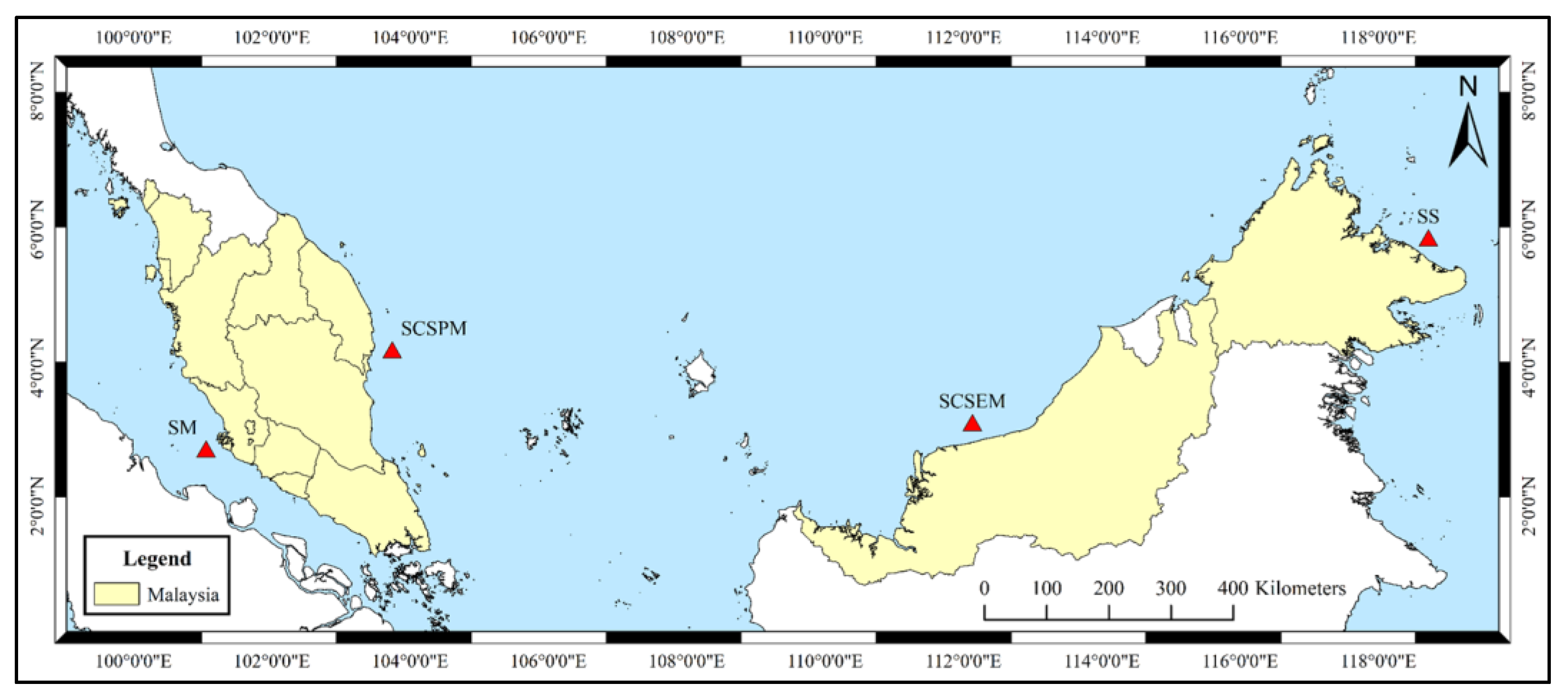
| Point | Location | Longitude | Latitude |
|---|---|---|---|
| SM | Malacca Strait | 101°3’8.57” E | 2°49’38.36” N |
| SCSPM | SCS—Peninsular | 103°44’34.45” E | 4°15’34.30” N |
| SCSEM | SCS—Sarawak | 112°7’52.34” E | 3°12’31.81” N |
| SS | Sulu Sea | 118°43’30.36” E | 5°52’49.73” N |
| Warming | Year | Strait of Malacca | SCS—Peninsular Malaysia | SCS—East Malaysia | Sulu Sea | ||||||||
|---|---|---|---|---|---|---|---|---|---|---|---|---|---|
| Sea Level (m) | Sea Level Change (mm) | Trend (mm/Year) | Sea Level (m) | Sea Level Change (mm) | Trend (mm/Year) | Sea Level (m) | Sea Level Change (mm) | Trend (mm/Year) | Sea Level (m) | Sea Level Change (mm) | Trend (mm/Year) | ||
| 1.5 °C | 2028 | 0.752 | 4.5 | 1.0 | 0.908 | 16.0 | 1.5 | 0.895 | 14.5 | 1.1 | 0.838 | 9.2 | 0.6 |
| 2.0 °C | 2043 | 0.757 | 10.0 | 0.5 | 0.912 | 20.2 | 0.6 | 0.903 | 21.5 | 0.7 | 0.844 | 15.4 | 0.5 |
| 2080 | 0.783 | 36.3 | 0.6 | 0.950 | 57.7 | 0.8 | 0.934 | 53.2 | 0.7 | 0.869 | 40.1 | 0.6 | |
| 2100 | 0.806 | 58.8 | 0.8 | 0.975 | 83.1 | 1.0 | 0.963 | 81.7 | 0.9 | 0.894 | 65.2 | 0.8 | |
Disclaimer/Publisher’s Note: The statements, opinions and data contained in all publications are solely those of the individual author(s) and contributor(s) and not of MDPI and/or the editor(s). MDPI and/or the editor(s) disclaim responsibility for any injury to people or property resulting from any ideas, methods, instructions or products referred to in the content. |
© 2023 by the authors. Licensee MDPI, Basel, Switzerland. This article is an open access article distributed under the terms and conditions of the Creative Commons Attribution (CC BY) license (https://creativecommons.org/licenses/by/4.0/).
Share and Cite
Azran, N.I.; Jeofry, H.; Chung, J.X.; Juneng, L.; Ali, S.A.S.; Griffiths, A.; Ramli, M.Z.; Ariffin, E.H.; Miskon, M.F.; Mohamed, J.; et al. Southern South China Sea Dynamics: Sea Level Change from Coupled Model Intercomparison Project Phase 6 (CMIP6) in the 21st Century. J. Mar. Sci. Eng. 2023, 11, 458. https://doi.org/10.3390/jmse11020458
Azran NI, Jeofry H, Chung JX, Juneng L, Ali SAS, Griffiths A, Ramli MZ, Ariffin EH, Miskon MF, Mohamed J, et al. Southern South China Sea Dynamics: Sea Level Change from Coupled Model Intercomparison Project Phase 6 (CMIP6) in the 21st Century. Journal of Marine Science and Engineering. 2023; 11(2):458. https://doi.org/10.3390/jmse11020458
Chicago/Turabian StyleAzran, Noah Irfan, Hafeez Jeofry, Jing Xiang Chung, Liew Juneng, Syamir Alihan Showkat Ali, Alex Griffiths, Muhammad Zahir Ramli, Effi Helmy Ariffin, Mohd Fuad Miskon, Juliana Mohamed, and et al. 2023. "Southern South China Sea Dynamics: Sea Level Change from Coupled Model Intercomparison Project Phase 6 (CMIP6) in the 21st Century" Journal of Marine Science and Engineering 11, no. 2: 458. https://doi.org/10.3390/jmse11020458