State Compensation for Maritime Autonomous Surface Ships’ Remote Control

Abstract

With the development of emerging techniques, maritime autonomous surface ships (MASS) have attracted much attention, and the remote control ships’ future seems promising. However, due to communication issues, ship–shore transmission faces the challenge of time delay. The use of the transmitted information without compensation could reduce the effectiveness of controlling or could cause the remote control to be unstable. To eliminate the negative effects of uncertain delays during navigation, an Augmented State Cubature Kalman Filter (AS-CKF) is proposed. First, the uncertainty of the transmission delays is modeled using a probability density function (PDF). Second, the ship’s states are updated and estimated using the delayed observed data, and then the real state of the ship is simultaneously corrected in the augmented state vector. In this way, the delay compensation problem becomes a one-step prediction problem. To test the proposed AS-CKF for MASS, we simulate scenarios with the remote control ship under different communication time delays. The results show improvements compared to the traditional CKF, EKF, or AS-EKF, which indicates the potential of the proposed methods in remote control MASS.

1. Introduction

With the development of artificial intelligence technologies, intelligent vehicles that integrate computer science, automation technology, and communication technology have become the research frontier in the field of high tech [1,2,3]. As an intelligent surface vehicle, maritime autonomous surface ships (MASS) are considered to be a useful platform in waterborne transportation, ocean surveying and mapping, and maritime security, among other fields [4,5]. Remote control ships that can be controlled by operators shoreside provide operators and managers with convenient, efficient, and free operation options, which have received much attention in recent years [6,7]. However, there may be challenges in implementing MASS remote control due to varying communication time delays. These time delays are frequently caused by issues such as with the status of the communication network or the communication distance between remote controllers and MASS [8]. In such cases, the signals obtained by the remote controllers cannot truly reflect the current state of the ship, thereby reducing the experience of controlling the ship or causing the ship to be unstable. Therefore, it is necessary to compensate for the delay in the navigation of MASS.

Many techniques have been proposed to estimate the system states, e.g., a family of Kalman Filters (KF). Extended Kalman Filter (EKF) is the most common filtering algorithm used to estimate the navigation state. EKF is used when KF cannot be applied to nonlinear systems. EKF maintains a low computational complexity, but the negligibility of higher-order terms of the nonlinear system in EKF will degrade the estimation accuracy [9,10]. Unscented Kalman Filter (UKF) and Cubature Kalman Filter (CKF) are two other popular methods for sampling filtering. UKF uses a series of sigma points to propagate the states and covariance matrix [9,11]. CKF computes integrals, such as nonlinear function times for Gaussian density [12,13]. Unlike UKF, which uses 2n + 1 unscented points to propagate the state and covariance matrix, CKF propagates the state and covariance matrix with 2n Cubature points. CKF thereby has a relatively lower computational load than UKF when the same matrix decomposition methods, such as singular value decomposition or the Cholesky method, are applied to UKF and CKF. For high-level systems, CKF has better stability and higher accuracy [14]. However, these filters do not consider the delay of the system in the design. When there is a delayed observation of the sensor, CKF cannot be applied.

In general, it is assumed that the measurement time is consistent with the filter time, but there is a time delay during the transmission of the filter measurement in some cases, such as remote control MASS. In such cases, the communication network quality and regional bandwidth, among other factors, cause a time delay during transmission of the measurement data collected by on-board sensors to the shore-based control center (SCC). The issue of delayed filter measurement availability is referred to as Out Of Sequence Measurement (OOSM) [15,16].

In order to solve the issue of estimation in the case of time-delayed observation, scholars have conducted related work. For a time delay that is known, the past state can be predicted by applying backward prediction of the current state. In such cases, Hua [17] proposed a multiple linear regression method to predict the network delay jitter for a networked teleoperation system, with the effectiveness of the proposed method being verified by simulation. Bar-Shalom [18] proposed an optimal and suboptimal algorithm for one-step delayed measurement. Chen et al. [19] improved the method so that it can be used in the case of multi-step delayed measurements. The literature verified that algorithms that work for one-step-lag OOSM also work for multi-step-lag OOSM.

For the time delay that is unknown, Kyuman Lee [20] estimated the delay of measurement by incorporating a parameter estimation technique into state estimation. However, since the delay itself is random, it is difficult to obtain a converged delay estimate in practical applications. Shijie Zhang [21] proposed a state estimation error compensation method to solve the decrease in positioning accuracy caused by communication delay in multi-robot systems. This study, however, only considers the invariable time delay. Choi, M [22] solved these delayed measurement problems with an augmented state Kalman filter, and the uncertainty of the delayed time was resolved based on the probability distribution of the delay. Considering the actual situation, an augmented EKF was proposed by Das B [23], and the method was applied to a telepresence robot system. Adachi R [24] proposed a maximum-likelihood estimation method for delay compensation, which addressed the delay problem by writing the observation equation as an observation with experiments and an observation equation without delay. This method was an augmented-matrix method. When augmenting the state, the state corresponding to the maximum delay needs to be calculated, which will cause the augmented state vector to widen. Furthermore, calculations with a large-sized vector may require additional extensive computational effort.

In order to reduce the computational complexity of the algorithm, and to improve its adaptability to the nonlinearity of the system, AS-CKF is proposed. AS-CKF is combined with the ideas of CKF and state augmentation in this paper. First, the augmented state is used to replace the original state, and the past state is updated through delayed observation. Second, the new predicted value of the current state is obtained from the corrected past state. To overcome dimension challenges, the uncertain delay is replaced by the distributed expectation, which reduces the extensive computational effort. Third, a set of simulation experiments is designed to simulate the performance of the algorithm when the uncertain time delay obeys the Gaussian distribution.

The rest of the paper is organized as follows: In Section 2, the state compensation for MASS is described and modelled. In Section 3, the original CKF and the CKF considering the uncertainty of time delay are introduced. Section 4 introduces the methodology for delayed measurement. In Section 5, the experimental framework is presented and the experiment results are analyzed and evaluated. Then, Section 6 concludes the paper.

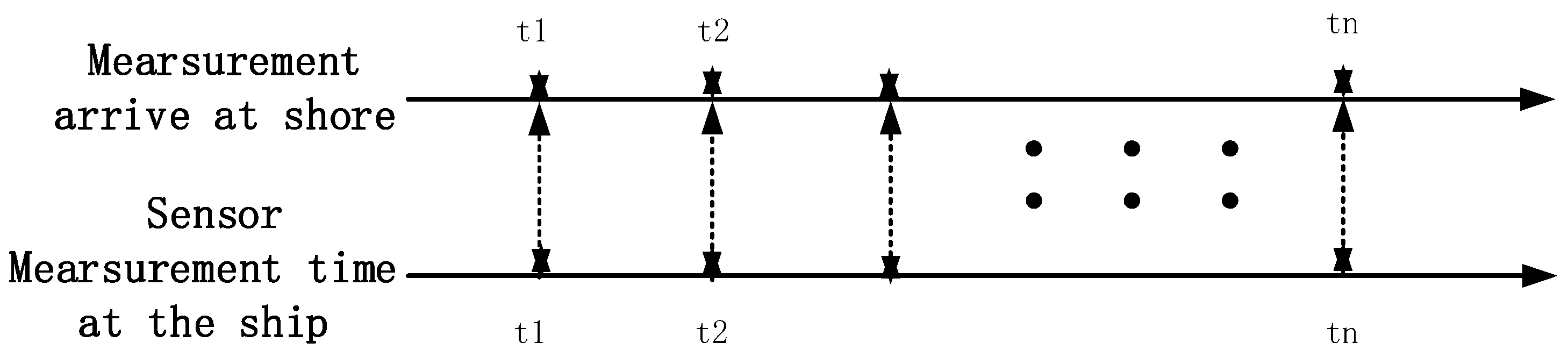
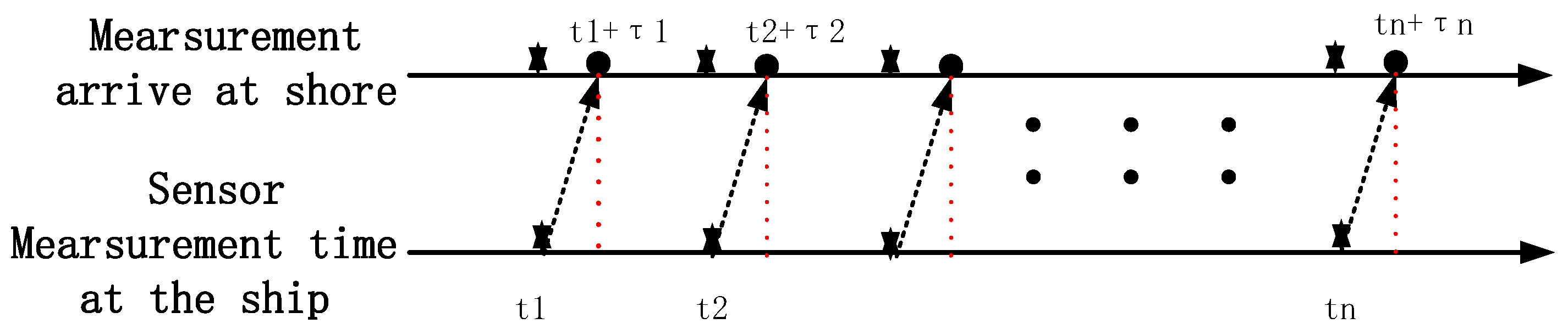
2. Problem Statement

When the MASS is remotely controlled, the ship’s movement status is not timely because of the communication delay due to network quality, communication distance, etc., causing challenges for the controllers and thus compromising their ability to control the ship safely. The kinematic model of a ship is defined as follows:

$$x_k=x_{k-1}+T_s(u_k\cos ({\psi }_k)-v\sin ({\psi }_k))$$

(1)

$$y_k=y_{k-1}+T_s(u_k\sin ({\psi }_k)+v\cos ({\psi }_k))$$

(2)

$${\psi }_k={\psi }_{k-1}+T_{s}r$$

(3)

where $x_k$,$y_k$ are the Cartesian coordinates of the ship, $u_k$ is surge velocity and $v_k$ is sway velocity, ${\psi }_k$ is yaw, $r$ is yaw rate, and $T_s$ is discrete sampling time.

In this study, we aim to estimate the motion state of the intelligent ship. For the general nonlinear discrete system, the system equation can be established as follows:

$$\{\begin{array}{c}{x}_k=f(x_{k-1},w_{k-1})\\ z_k=h(x_k,v_k)\end{array}$$

(4)

where $x_k\in R^n$ is a $n\times 1$ state vector, $z_k\in R^m$ is an $m\times 1$ observation vector, $w_{k-1}\in R^n$ is system noise, and $v_k\in R^m$ is an observation vector; both noises are assumed to be Gaussian white noise sequences with zero mean. Additionally, $E\left[w_{k-1}{w}_{k-1}^T\right]=Q_{k-1}$, $E\left[v_k{v}_k^T\right]=R_k$; $f(•)$ is the dynamics model of the system; and $h(•)$ is the measurement function.

It can be seen from the observation equation in Equation (4) that the observation vector $z_k$ contains information about $x_k$. It also shows that the timing of the state information perceived by the sensor is consistent with the time at which the information is used for filtering (as shown in Figure 1). However, this may not be the case in the remote control scenario.

When the ship is remotely controlled by a shoreside control center (SCC), the perceived information by ship-side sensors may not be used simultaneously in the SCC due to the time delay. The delay arises from the communication time between the ship and the SCC and the algorithm processing time, among other factors. Therefore, measurement time will be different from filter time, as shown in Figure 2. In this case, the measurement equation is rewritten as follows:

$$z_k=h(x_{k-{\tau }_k},v_{k-{\tau }_k})$$

(5)

where ${\tau }_k$ represents the step of the delay of measurement data. The measurement $z_k$ is related to the step before ${\tau }_k$; the current state cannot be corrected by the received measurement data. If the delay time is precise, the state corresponding to the measurement can be estimated. However, in a real state, the time delays ${\tau }_k$ may not be precisely measured due to various delays, namely, feedback delay and transmission delay, and data packet drop-outs over the Internet. Hence, the arrival time in filter measurement time durations will be random, as shown in Figure 3.

3. Improved Cubature Kalman Filter Considering Uncertain Delays

3.1. Original Cubature Kalman Filter

The derivation of the Cubature Kalman Filter (CKF) utilizes the third-degree spherical–radial cubature rule, and the detailed derivation process can be found in [13,25]. This article only gives a brief introduction to the algorithm. For a nonlinear system, e.g., Equation (4), the CKF is calculated with the following steps:

Step 1: Initialization

$${\widehat{x}}_0=E[x_0],P_0=E[(x_0-{\widehat{x}}_0){(x_0-{\widehat{x}}_0)}^T]$$

(6)

where $E$ is the expectation operator.

Step 2: Time update

$$S_{k-1/k-1}=chol(P_{k-1/k-1})$$

(7)

$$X_{i,k-1/k-1}=S_{k-1/k-1}{\xi }_i+{\widehat{x}}_{k-1/k-1}i=1,2,3,\cdots ,2n$$

(8)

where chol represents the Cholesky decomposition method, $S$ is the square root of covariance matrix $P$, ${\widehat{x}}_{k-1/k-1}$ is the estimated value of the previous, i is the Cubature point serial number, and ${\xi }_i$ stands for column i of $\xi$ that is formulated as:

$$\xi =\sqrt{n}\left[\begin{array}{cccccccc}1& & & & -1& & & \\ & 1& & & & -1& & \\ & & \ddots & & & & \ddots & \\ & & & 1& & & & -1\end{array}\right]$$

In matrix $\xi$, only one element in each column is 1 or −1, and the other elements are 0.

$$X_{i,k/k-1}^{\ast }=f(X_{i,k-1/k-1})$$

(9)

$${\widehat{x}}_{k/k-1}=\frac{1}{2n}{\displaystyle \sum _{i=1}^{2n}{X}_{{}_{i,k/k-1}}^{*}}$$

(10)

$$P_{k/k-1}=\frac{1}{2n}{\displaystyle \sum _{i=1}^{2n}(X_{i,k/k-1}^{*}{X}_{i,k/k-1}^{*T}}-{\widehat{x}}_{k/k-1}{\widehat{x}}_{k/k-1}^T)+Q_{k-1}$$

(11)

where $X_{i,k/k-1}^{}$ is the Cubature point generated from states, ${(•)}_{i,k/k-1}^{}$ represents the one-step prediction of relevant parameters, and the symbol ${\displaystyle \sum _{}^{}}$ represents the accumulation operation.

Step 3: Measurement update

$$P_{k/k-1}=S_{k/k-1}{S}^T{}_{k/k-1}$$

(12)

$$X_{i,k/k-1}=S_{k/k-1}{\xi }_i+{\widehat{x}}_{k/k-1}$$

(13)

$$Z_{i,k/k-1}=h(X_{i,k/k-1})$$

(14)

$${\widehat{z}}_{k/k-1}=\frac{1}{2n}{\displaystyle \sum _{i=1}^{2n}{Z}_{i,k/k-1}}$$

(15)

$${\eta }_k=Z_k-{\widehat{z}}_{k/k-1}$$

(16)

$$P_{zz,k/k-1}=\frac{1}{2n}{\displaystyle \sum _{i=1}^{2n}(Z_{i,k/k-1}^{}{Z}_{i,k/k-1}^T}-{\widehat{z}}_{k/k-1}{\widehat{z}}_{k/k-1}^T)+R_k$$

(17)

$$P_{xz,k/k-1}=\frac{1}{2n}{\displaystyle \sum _{i=1}^{2n}(X_{i,k/k-1}^{}{Z}_{i,k/k-1}^T}-{\widehat{x}}_{k/k-1}{\widehat{z}}_{k/k-1}^T)$$

(18)

where $Z_{i,k/k-1}^{}$ represents the Cubature point generated from measurements.

Step 4: State update

$$K_k=P_{zz,k/k-1}{P}^{-1}{}_{xz,k/k-1}$$

(19)

$${\widehat{x}}_{k/k}={\widehat{x}}_{k/k-1}+K_k(z_k-{\widehat{z}}_{k/k-1})$$

(20)

$$P_{k/k}=P_{k/k-1}-K_k{P}_{zz,k/k}{K}_k^T$$

(21)

where $K_k$ is the gain of the CKF, ${\widehat{x}}_{k/k}$ is the state after updating, and $P_{k/k}$ is the error-covariance of state ${\widehat{x}}_{k/k}$.

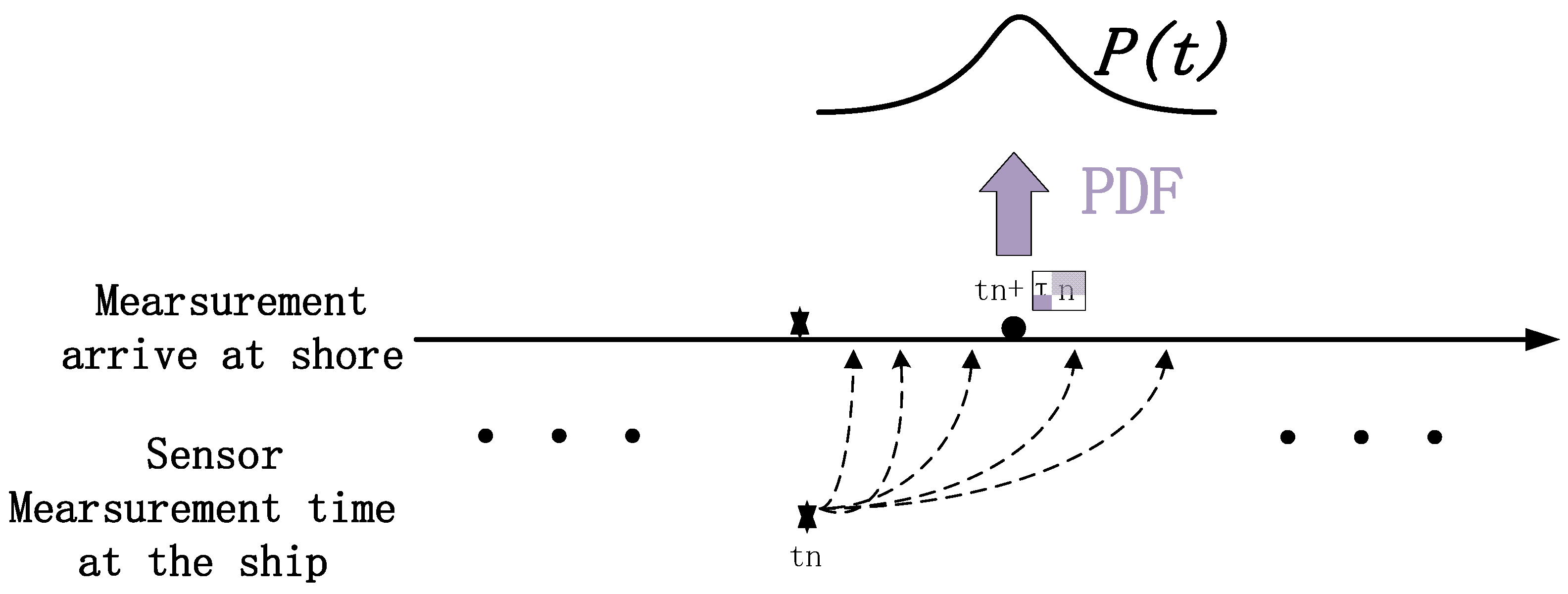
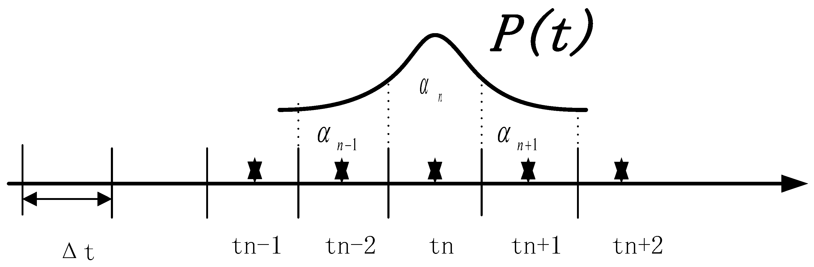
3.2. Improved CKF Considering Uncertain Time Delay

The delay time is modeled as a PDF to solve the issue that the delay cannot be accurately obtained and is random. When a measurement arrives in the filter, the probability of a step of time delay can be calculated by integrating the PDF.

The probability that the measured value is in the n-th time step can be calculated as:

$$\begin{array}{cc}{\alpha }_n& =P((t_n-\frac{\Delta t}{2})\le t\le (t_n+\frac{\Delta t}{2}))\hfill \\ & ={\displaystyle {\int }_{t_n-\frac{\Delta t}{2}}^{t_n+\frac{\Delta t}{2}}p(t)}dt\hfill \end{array}$$

(22)

where $P(•)$ means a probability, and $p(•)$ is the probabilistic density functions. Suppose that the measurement value $z(k)$ is given, and a correspondence $c_n$ means that the value $z(k)$ is in the n-th time step, a probability that represents the measurement is in the n-th step is written as:

$$P(c_n|z(k))={\alpha }_n$$

(23)

Considering the correspondence $c_n$, a state estimator can be derived:

$$\begin{array}{cc}{\widehat{x}}_{k/k}& =E\left\{x(k)|z(k)\right\}\hfill \\ & ={\displaystyle \sum _{n}P(c_n|z(k))}E\left\{x(k)|z(k),c_n\right\}\hfill \\ & ={\displaystyle \sum _n{\alpha }_n}E\left\{x(k)|z(k),c_n\right\}\hfill \end{array}$$

(24)

${\widehat{x}}_{k/k}$ is the expectation of the current state when there is a delay in the measurement $z(k)$. From Figure 4, we can see that the total number of $c_i$ will affect the computation of the algorithm. To reduce the amount of computation, we consider such average delay (modeled by PDF) as a continuous input to the system, which will allow us to calculate only one $E$, i.e., one status update and corresponding multiple one-step predictions. Based on the framework of CKF, the current state can be calculated by augmenting several steps of the past state. The detailed calculation process is provided in Section 4.2.

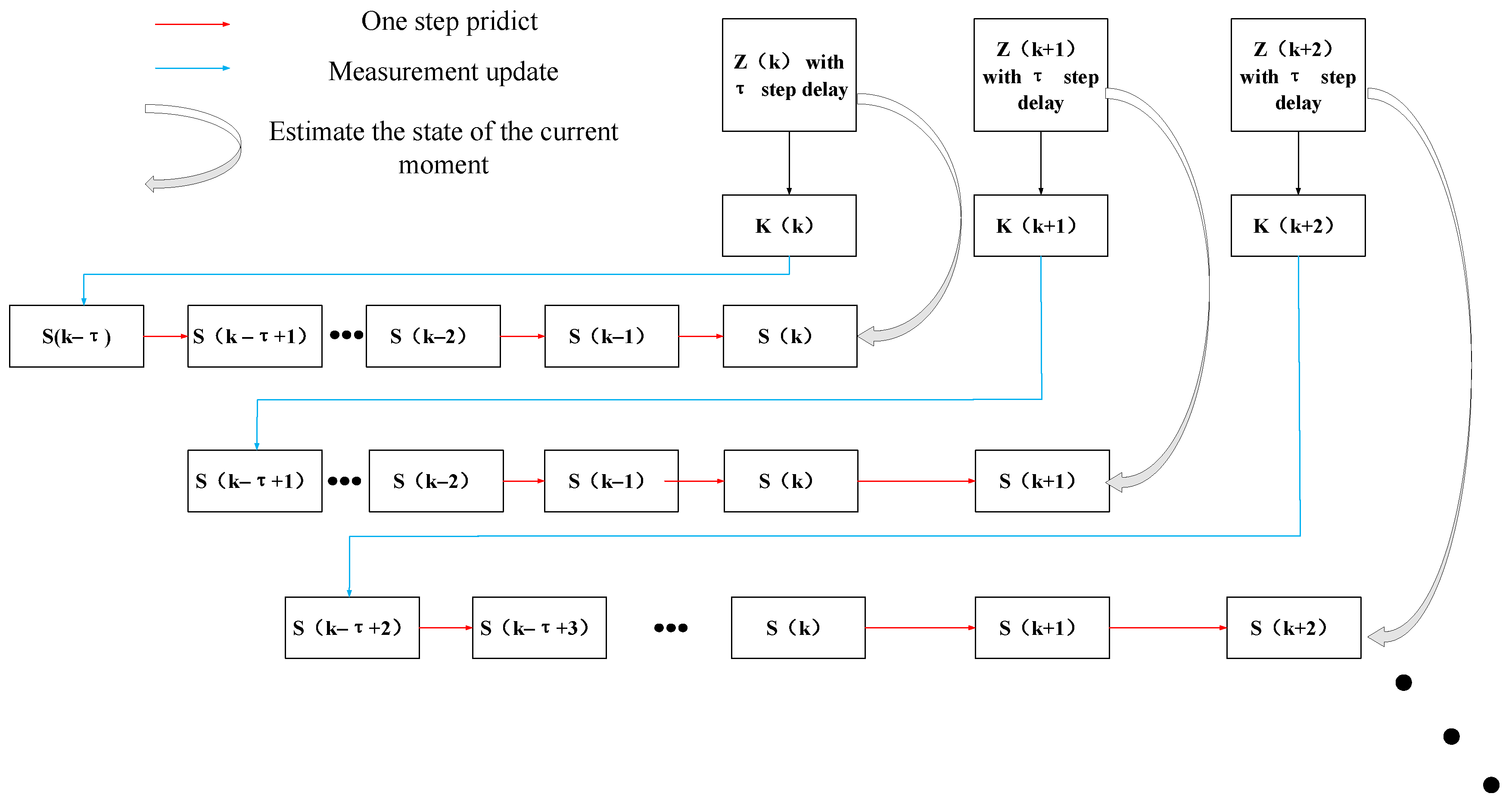
4. Delay-Compensated State Estimation for MASS

4.1. Framework of Method

In the scenario of remote control, the information on the MASS movement status received by the shore-based controller may not be synchronized with the information generated by the MASS. The currently received measurement information cannot directly estimate the current state. Thus, the present state and the past states are combined into several augmented state vectors, which are used to estimate the ship’s true position.

Figure 5 illustrates a flow diagram of the proposed algorithm. The current measurement state, which contains information on the past states, directly corrects the augmented state vector. In this way, the past state is updated using the delayed measurement data and the current state is simultaneously corrected in the augmented state vector. The estimation of current state consists of two parts: the first part is the estimation of the corresponding past state, and the other part is given by multiple one-step predictions. Figure 5 illustrates a flow diagram of the proposed algorithm.

4.2. Augmented State Cubature Kalman Filter (AS-CKF)

We solve the problem of ship-state estimation under observation delay using an augmented state CKF. We combine the current state and past state into a new system state to estimate the true position of the ship. In a time-delay system, by updating the augmented state with the measured value of the past state information, the past state can be updated directly, and then the current state can be further corrected according to the updated past state. Taking one-step delay as an example, the system equation is rewritten as follows:

$$x_{k-1}^{aug}=\left[\begin{array}{c}{x}_k\\ x_{k-1}\end{array}\right]=\left[\begin{array}{c}f(x_{k-1},w_{k-1})\\ x_{k-1}\end{array}\right]=\left[\begin{array}{cc}{\Phi }_{k/k-1}& 0\\ 0& {\Phi }_{k-1/k-2}\end{array}\right]\left[\begin{array}{c}{x}_{k-1}\\ x_{k-2}\end{array}\right]+\left[\begin{array}{cc}{\Gamma }_{k/k-1}& 0\\ 0& {\Gamma }_{k-1/k-2}\end{array}\right]\left[\begin{array}{c}{w}_{k/k-1}\\ w_{k-1/k-2}\end{array}\right]$$

(25)

where ${()}_{}^{aug}$ is the augmented state vector, ${\Phi }_{k/k-1}=\frac{\partial f(x,w)}{\partial x}{|}_{x=x_{k-1}}$, ${\Gamma }_{k/k-1}=\frac{\partial f(x,w)}{\partial w}{|}_{w=w_{k-1}}$. Similarly, ${\Phi }_{k-1/k-2}$, ${\Gamma }_{k-1/k-2}$ can be calculated using the following measurement equation:

$$z_{k-1}^{aug}=\left[\begin{array}{c}0\\ z_{k-1}\end{array}\right]=h([0,I]\left[\begin{array}{c}{x}_k\\ x_{k-1}\end{array}\right],\left[\begin{array}{c}{v}_k\\ v_{k-1}\end{array}\right])=\left[\begin{array}{cc}0& 0\\ 0& H_{k-1/k-2}\end{array}\right]\left[\begin{array}{c}{x}_{k-1}\\ x_{k-2}\end{array}\right]+\left[\begin{array}{c}0\\ w_{k-1/k-2}\end{array}\right]$$

(26)

where $H_{k-1/k-2}=\frac{\partial h(x,w)}{\partial x}{|}_{x=x_{k-2}}$.

For the system represented by Equations (25) and (26), Equations (5) and (7) are rewritten as follows:

$$P_{k-1/k-1}^{aug}=\left[\begin{array}{cc}{S}_{k-1/k-1}& 0\\ A& S_{k-2/k-2}\end{array}\right]\left[\begin{array}{cc}{S}_{{}_{k-1/k-1}}^T& A^T\\ 0& S_{{}_{k-2/k-2}}^T\end{array}\right]$$

(27)

$$X_{i,k-1/k-1}^{aug}=\left[\begin{array}{cc}{S}_{k-1/k-1}& 0\\ A& S_{k-2/k-2}\end{array}\right]{\xi }_i^{aug}+\left[\begin{array}{c}{\widehat{x}}_{k-1/k-1}\\ {\widehat{x}}_{k-1/k-2}\end{array}\right],{\xi }_{}^{aug}=\sqrt{2n}\left|\begin{array}{cccc}{I}_{n\times n}& 0& -I_{n\times n}& 0\\ 0& I_{n\times n}& 0& -I_{n\times n}\end{array}\right|$$

(28)

If let $X_{k-1/k-1}^{aug}=\left[\begin{array}{cccc}{X}_{1,k-1/k-1}^{aug}& X_{2,k-1/k-1}^{aug}& •••& X_{i,k-1/k-1}^{aug}\end{array}\right]$,then have:

$$X_{k-1/k-1}^{aug}=\left[\begin{array}{cc}{\left[\begin{array}{c}{\widehat{x}}_{k-1/k-1}\\ {\widehat{x}}_{k-1/k-2}\end{array}\right]}_n+\left[\begin{array}{cc}{S}_{k-1/k-1}& 0\\ A& S_{k-2/k-2}\end{array}\right]& {\left[\begin{array}{c}{\widehat{x}}_{k-1/k-1}\\ {\widehat{x}}_{k-1/k-2}\end{array}\right]}_n-\left[\begin{array}{cc}{S}_{k-1/k-1}& 0\\ A& S_{k-2/k-2}\end{array}\right]\end{array}\right]$$

where ${\left[X\right]}_n$ represents an $n\times n$-dimensional matrix constructed by repeating $n$times column vector, and $X$, $X_{i,k-1/k-1}^{aug}$ represents the i-th column vector of $X_{k-1/k-1}^{aug}$.

Combining Equations (9) and (25), we get:

$$X_{i,k/k-1}^{\ast aug}=\left[\begin{array}{c}{X}_{{}_{i,k/k-1}}^{*}\\ X_{{}_{i,k-1/k-2}}^{*}\end{array}\right]=\left[\begin{array}{cc}{\Phi }_{k/k-1}& 0\\ 0& {\Phi }_{k-1/k-2}\end{array}\right]X_{i,k-1/k-1}^{aug}$$

(29)

$${\widehat{x}}_{k/k-1}^{aug}=\frac{1}{2n}{\displaystyle \sum _{i=1}^{2n}\left[\begin{array}{c}{X}_{{}_{i,k/k-1}}^{*}\\ X_{{}_{i,k-1/k-2}}^{*}\end{array}\right]}=\left[\begin{array}{c}{\widehat{x}}_{k/k-1}\\ {\widehat{x}}_{k-1/k-2}\end{array}\right]$$

(30)

So, we can calculate time update:

$$P_{k/k-1}^{aug}=\frac{1}{2n}{\displaystyle \sum _{i=1}^{2n}(X_{i,k/k-1}^{aug}{X}_{i,k/k-1}^{augT}}-{\widehat{x}}_{k/k-1}^{aug}{\widehat{x}}_{k/k-1}^{augT})+Q_{k-1}^{aug}$$

(31)

$${\widehat{x}}_{k/k-1}^{aug}=\frac{1}{2n}{\displaystyle \sum _{i=1}^{2n}\left[\begin{array}{c}{X}_{{}_{i,k/k-1}}^{*}\\ X_{{}_{i,k-1/k-2}}^{*}\end{array}\right]}=\left[\begin{array}{c}{\widehat{x}}_{k/k-1}\\ {\widehat{x}}_{k-1/k-2}\end{array}\right]$$

(32)

Pay attention to the change of the size of dimension n in the calculation. Since a new augmented state is constructed and the historical state is included in the state, the dimension of the new augmented state should be twice the original state, that is, n will also be doubled. Combining Equations (12)–(21) and (26), a state update can be calculated:

$$\begin{array}{cc}{P}_{{}_{zz,k/k-1}}^{aug}& =\frac{1}{2n}{\displaystyle \sum _{i=1}^{2n}\left[\begin{array}{c}0\\ Z_{i,k/k-1}^{}\end{array}\right]\left[\begin{array}{cc}{0}^T& Z_{i,k/k-1}^T\end{array}\right]}-\left[\begin{array}{c}0\\ {\widehat{z}}_{k/k-1}\end{array}\right]\left[\begin{array}{cc}{0}^T& {\widehat{z}}_{k/k-1}^T\end{array}\right]+\left[\begin{array}{cc}0& 0\\ 0& R_{k-1}\end{array}\right]\hfill \\ & =\left[\begin{array}{cc}0& 0\\ 0& P_{zz,k-1/k-2}\end{array}\right]\hfill \end{array}$$

(33)

$$K_k^{aug}=\left[\begin{array}{cc}0& 0\\ 0& K_{k-1}\end{array}\right]$$

(34)

$${\widehat{x}}_{k/k}^{aug}=\left[\begin{array}{c}{\widehat{x}}_k\\ {\widehat{x}}_{k-1}\end{array}\right]=\left[\begin{array}{c}{\widehat{x}}_{k/k-1}\\ {\widehat{x}}_{k-1/k-2}\end{array}\right]+\left[\begin{array}{c}0\\ K_{k-1}(z_k-{\widehat{z}}_{k/k-1})\end{array}\right]$$

(35)

It can be seen from the equation of state update that after the past state is updated with the time-delay observation, a one-step prediction is performed to estimate the current state.

5. Simulation and Analysis

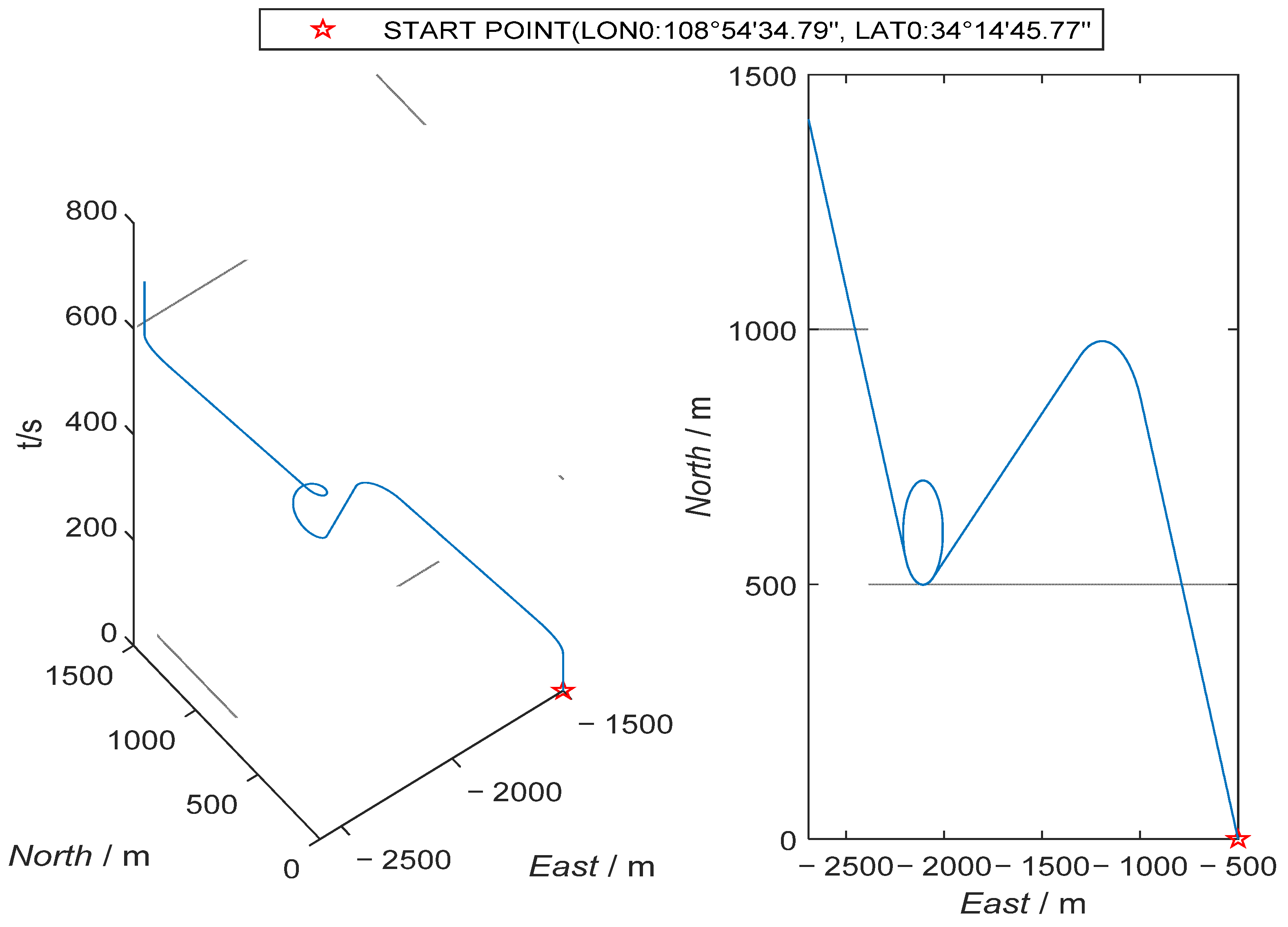
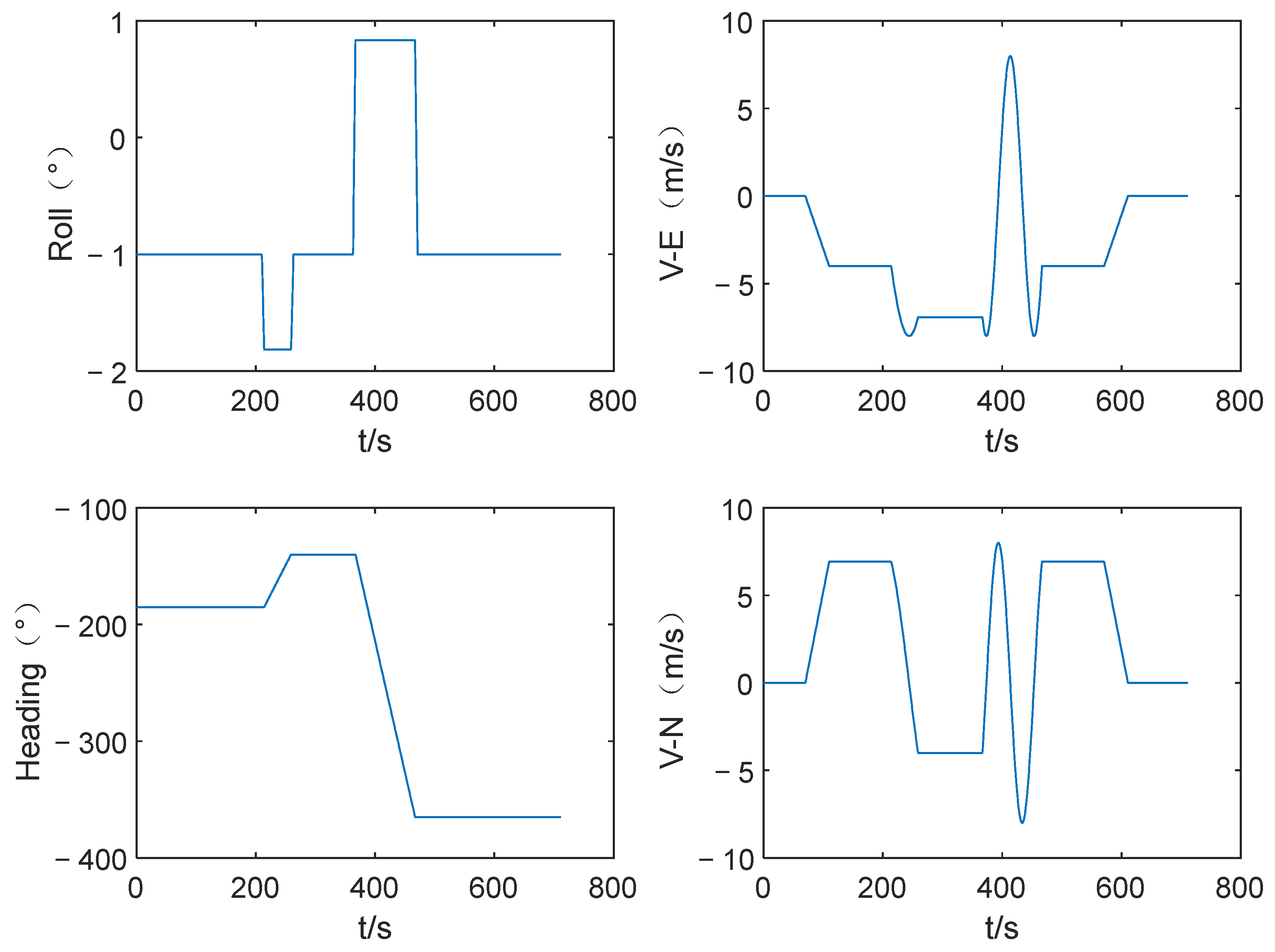
5.1. Setups

In this section, a set of simulation experiments will be used to verify that the proposed algorithm can track the ship within various maneuvering states under the condition of time delay. When simulating the running track and motion state of the ship, the common motion behaviors of the ship are considered, including acceleration, deceleration, uniform speed, left rotation, right rotation, etc. The ship’s general maneuvering characteristics are considered in the design of the simulation experiment, and the maximal sailing speed and turning radius of the ship are limited. In this simulation, the simulated ship has maximal speed of 16 knots, and the length of ship is 40 m.

Table 1. Ship motion state and related parameter design.

Time (s)	Status of Smart Ships	Changes in Motion Parameters
(0,70]	System initialization and initial alignment	-
(70,110]	Accelerate (m/s2)	Forward acceleration = 0.2 m/s2
(110,200]	Straight ahead	Forward acceleration = 0 m/s2
(200,204]	Rolling left (°/s)	Roll rate = −1.836°/s
(204,249]	Turning left (°/s)	Heading rate = 2°/s Roll rate = 0°/s
(249,253]	Rolling right (°/s)	Heading rate = 0°/s Roll rate = 1.836°/s
(253,343]	Straight ahead (°/s)	Roll rate = 0°/s
(343,347]	Rolling right (°/s)	Roll rate = 4.12°/s
(347,447]	Turning right (°/s)	Heading rate = 4.5°/s Roll rate = 0°/s
(447,451]	Rolling left (°/s)	Heading rate = 0°/s Roll rate = −4.12°/s
(451,541]	Straight ahead (°/s)	Roll rate = 0°/s
(541,581]	Decelerate (m/s2)	Forward acceleration = −0.2 m/s2
(581,661]	Still	Forward acceleration = 0 m/s2

shows the specific process of trajectory simulation, and its motion trajectory is shown in Figure 6. Figure 7 presents the ship’s changes of velocity and attitude. In this simulation experiment, the sampling frequency of IMU is set to 50 Hz, the sampling frequency of GPS is 1 Hz, and other parameter settings are shown in

Table 2. Simulation parameter.

	Parameter	Value
Initial position error	East (m) North (m)	1 1
Initial speed error	East (m/s) North (m/s)	0.1 0.1
Initial attitude error	Roll (arcsec)	30
	Pitch (arcsec)	−30
	Heading (arcmin)	30
Parameters of the gyroscope	Constant bias (°/h) Random walk ($°/\sqrt{\mathrm{h}}$)	0.05 0.005
Parameters of accelerometer	Constant bias (ug) Random walk (ug/$\sqrt{\mathrm{HZ}}$)	400 20
GPS noise	Noise of Position (m) Noise of velocity (m/s)	(1, 1, 3) (0.1, 0.1, 0.1)
Delay parameter setting	Gaussian distribution (μ,σ)	Μ = (10, 20, 40, 100), σ = 1/5μ

. By superimposing the time delay of the IMU and GPS data generated by the simulation to simulate the time when the remote driver obtains the sampled data, five groups of time delays are introduced, which obey the following Gaussian distribution: N(μ, σ), where σ = 1/5μ, μ = (10,20,40,100).

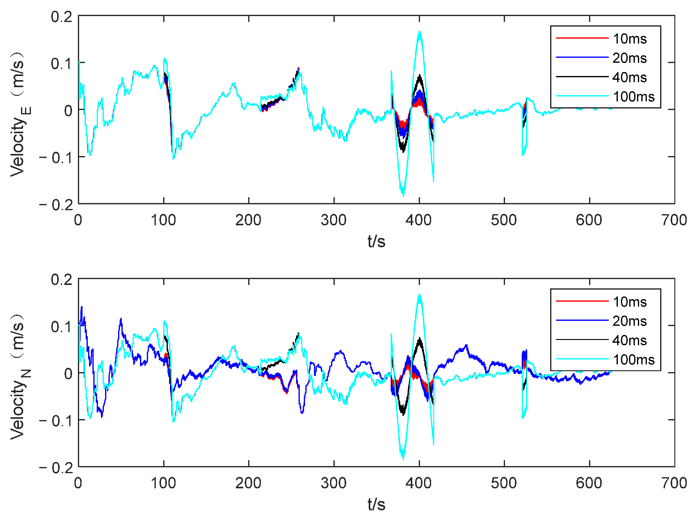
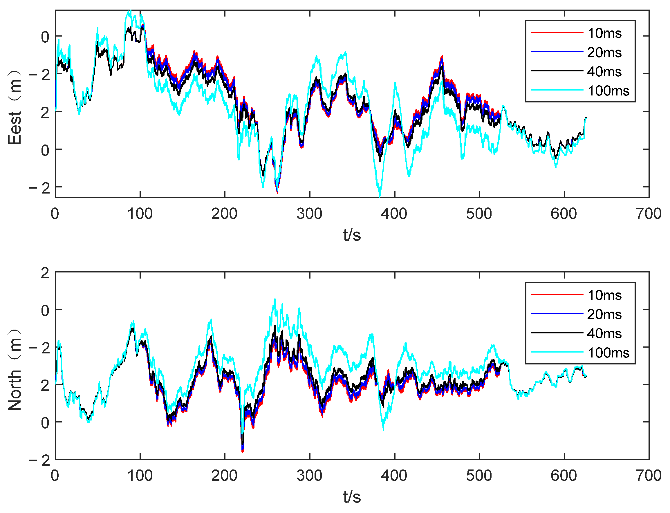
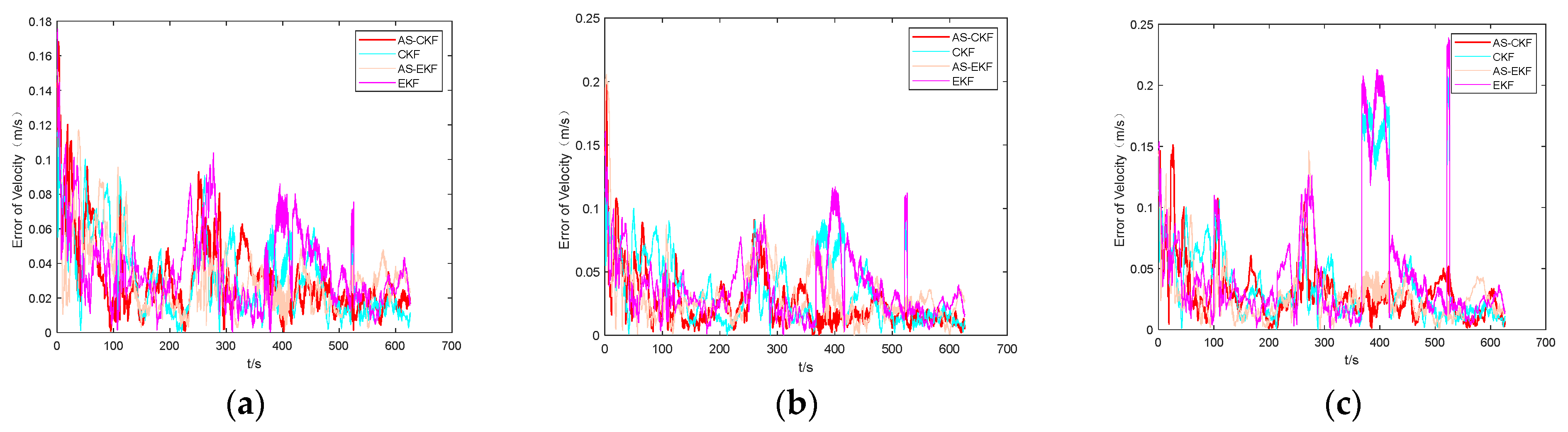
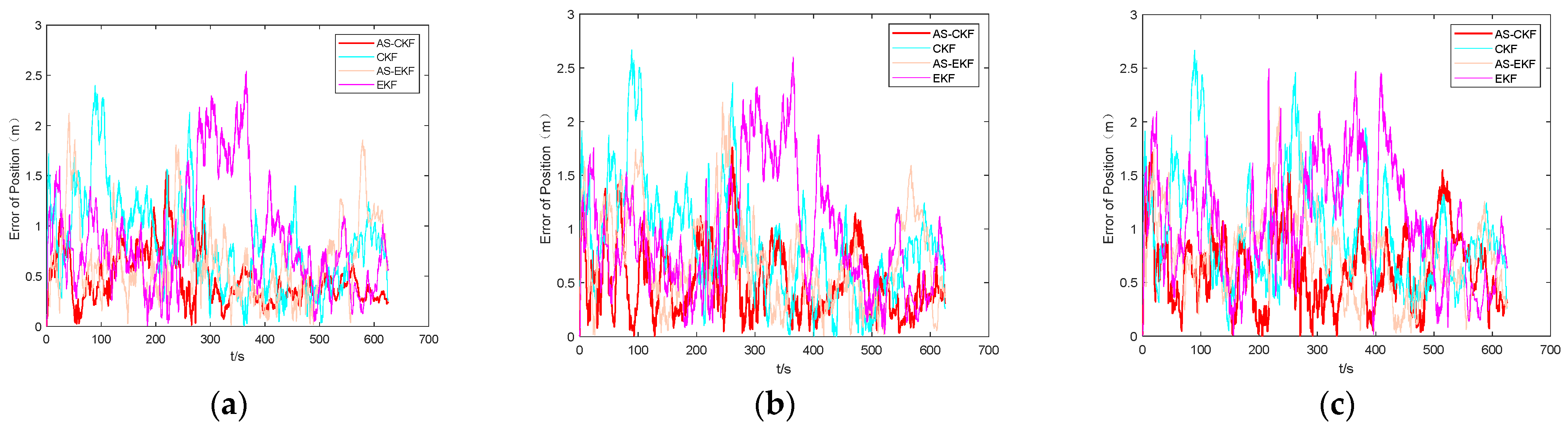
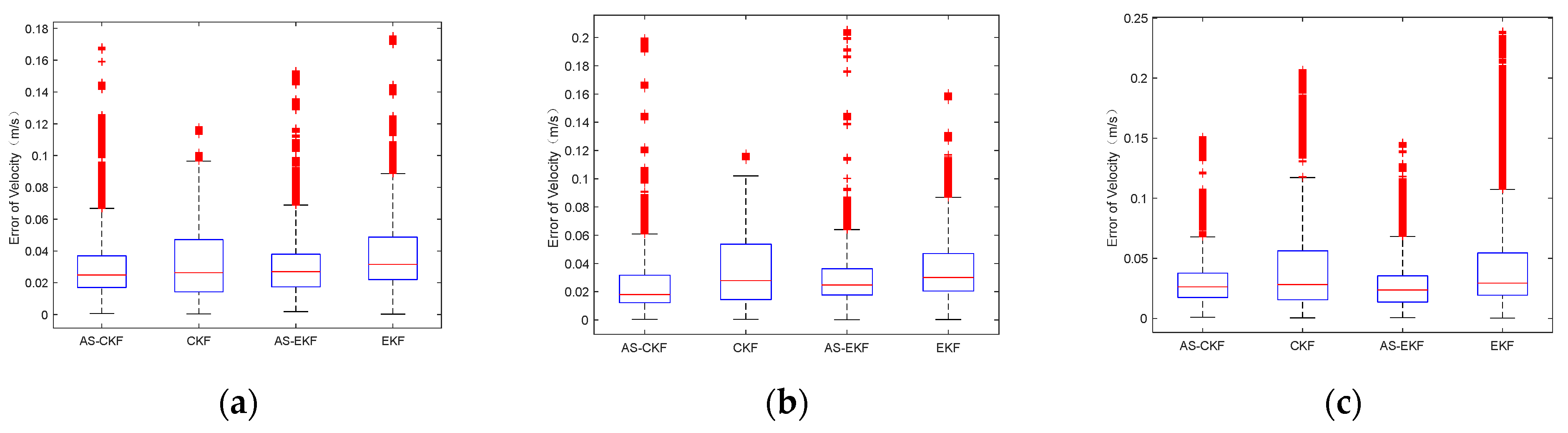
5.2. Simulation Results

Figure 8 and Figure 9 show the filtering conditions of the Cubature Kalman filter under different delay conditions. It can be seen from the results that the CKF cannot handle the error caused by the delay very well. It is actually an estimation of a certain state in the past, where the existence of time delay will introduce new errors. At (70, 110], (353,451], and (541,581], there is a significant increase in error, and it continues to maneuver at 360~470. In this case, the error increases significantly, which shows that the delay error reduces the dynamic performance of the system. With the aforementioned method, the past state is updated through the observation with time delay, and then the current state is predicted to solve the influence of the time delay on the filtering state.

The AS-CKF proposed in this paper is used to estimate the state of MASS under delay τ = 20 ms, 40 ms, and 100 ms, and is compared with the filtering results of CKF, EKF, and AS-EKF. The results are shown in Figure 10, Figure 11, Figure 12 and Figure 13. It can be seen from the results that the all algorithms can accurately estimate the state of velocity and position under the condition of uniform linear motion. This is because the speed of the ship does not change when the ship is moving in a straight line at a constant speed. In this case, updating the current state with delayed measurements will not introduce new errors. However, when accelerating or continuously turning, errors will be introduced in the system if we directly use the delayed measurement. It can be seen that estimation of CKF and EKF have obvious errors when the ship makes a circular motion. AS-EKF and the algorithm proposed in this paper can still ensure an accurate estimation of speed in the same scenario. In terms of the comparison of position accuracy, the proposed method in this paper is superior to other algorithms in the accuracy of position estimation, which is most obvious at 100 ms.

The root mean square errors (RMSE) of the three algorithms, CKF, AS-EKF, and AS-CKF, for position and speed are compared, as shown in

Table 3. RMSE error of velocity (m/s).

Average Delay in Time (ms)	RMSE			Improvement	Improvement
	CKF	AS-EKF	AS-CKF	Compared with CKF (%)	Compared with AS-EKF (%)
20	0.02122	0.0200	0.0194	9.38	<5
40	0.02530	0.0199	0.0187	28.06	6.9
100	0.02690	0.0210	0.0190	26.92	10.52

and

Table 4. RMSE error of velocity(m).

Average Delay in Time (ms)	RMSE			Improvement	Improvement
	CKF	AS-EKF	AS-CKF	Compared with CKF (%)	Compared with AS-EKF (%)
20	0.5033	0.4389	0.4379	13.01	<5
40	0.5798	0.4577	0.4424	23.78	<5
100	0.6395	0.4845	0.4254	33.41	13.89

. Both AS-EKF and the proposed algorithm can estimate the real state of the ship in a time-delay scenario, but the latter has higher accuracy. The proposed algorithm can maintain an error of 0.02 m/s in velocity and within 0.5 m in position estimation. When the delay is 20 ms, the accuracy of the algorithm is improved minimally compared to AS-EKF. When the delay reaches 100 ms, the accuracy of the proposed algorithm is significantly better than AS-EKF, and the accuracy of positioning and velocity are both improved by more than 10%. Compared with the CKF algorithm, the algorithm proposed in this paper has a greater improvement. Specifically, the accuracy of positioning and velocity estimation are improved by 9.38% and 11.01%, respectively. The estimation accuracy of positioning and speed with 40 ms delay are improved by 28.06% and 27.04%, respectively. The estimation accuracy of positioning and speed with 100 ms delay are improved by 26.96% and 33.41%, respectively. The accuracy of positioning and velocity estimation at 40 ms and 100 ms are increased mainly because the error of CKF algorithm increases under this condition.

5.3. Discussion

The delay-compensated state estimation approach successfully estimated the ship’s true position during navigation and compensated for the time delay from the measurement data as described in preceding sections. During the experiments we used the ship’s original simulation parameters, and the general maneuvering characteristics of the ship were considered in the design of the simulation experiment, so that the algorithm proposed in this paper is applicable to the remote control ship scenario.

We combined the current state and the past state into a new system state to estimate the true position of the ship. The current measurement state, which contains information on the past states, directly corrects the augmented state vector. In this way, the past state was updated using the delayed measurement data, and the current state was simultaneously corrected in the augmented state vector.

By comparing it with the existing EKF, CKF, and AS-EKF techniques for estimating a ship’s true position, we showed that our delay-compensated AS-CKF approach improves the estimation of ship positions in scenarios with delayed noisy sensor measurements. The traditional state estimation methods, such as EKF and CKF, are not suitable when there is time delay in the system’s observation. Estimating the current state through time-delayed observations will produce a large error, especially if the ship is maneuvering. Compared to AS-EKF, the CKF framework enables the method proposed in this paper to obtain a better dynamic performance in nonlinear systems.

The application of this method requires us to assume prior information, such as the expectation of delay distribution and use that expectation to address the delay uncertainty. Applying the algorithm proposed in this paper requires less delay. Otherwise, the dimension of the augmented state will be substantial, which is difficult to achieve in engineering. This method does not discuss the performance of the sensing device in different usage scenarios. For example, when the carrier is maneuvering, the accuracy of the sensing value will decrease with the increase in the nonlinearity of the system, which will directly affect the filtering accuracy.

The proposed algorithm can effectively estimate the state of the ship under the condition of time delay. By enlarging the states, we can update the past states with the observation quantity and time delay and estimate the current states with the updated state quantity and maintain a high estimation accuracy for the uncertain delay.

6. Conclusions

In this paper, a delay-compensated state estimation approach for a remote control ship with uncertain delayed navigation measurement was presented. By augmenting the state in CKF and introducing the historical state into the state, the historical state can be updated through the observation with delay. The current state then can be predicted through the updated historical state. Modeling the uncertain delay means the algorithm does not need to explicitly know the delay at each moment to achieve the state estimation, and by using the average of the modeled delay as the input of the system, the challenge of calculating too many states is avoided and the computational complexity of the algorithm is reduced. To demonstrate and verify this method, scenarios with varying transmission time delays were simulated and it was shown that the proposed method reduced the observed errors compared to the original CKF, EKF, and AS-EKF.

This study made some assumptions, such as the white noise assumption, the accurate delay distribution modeling, etc. To apply the proposed method in practical scenarios, further studies are needed. For instance, the performance of AS-CKF has been insufficiently explored, ship dynamics are unknown, and sensing device errors are unknown.

References

1. Felski, A.; Zwolak, K. The Ocean-Going Autonomous Ship-Challenges and Threats. J. Mar. Sci. Eng. 2020, 8, 41. [Google Scholar] [CrossRef] [Green Version]
2. Huang, Y.M.; Chen, L.Y. Generalized velocity obstacle algorithm for preventing ship collisions at sea. Ocean Eng. 2019, 173, 142–156. [Google Scholar] [CrossRef]
3. Chang, C.H.; Kontovas, C.; Yu, Q.; Yang, Z.L. Risk assessment of the operations of maritime autonomous surface ships. Reliab. Eng. Syst. Saf. 2021, 207, 107324. [Google Scholar] [CrossRef]
4. Fan, C.L.; Wrobel, K.; Montewka, J.; Gil, M.; Wan, C.P.; Zhang, D. A framework to identify factors influencing navigational risk for Maritime Autonomous Surface Ships. Ocean. Eng. 2020, 202, 107188. [Google Scholar] [CrossRef]
5. Wang, C.; Zhang, X.; Li, R.; Dong, P. Path Planning of Maritime Autonomous Surface Ships in Unknown Environment with Reinforcement Learning. In Proceedings of the 4th International Conference on Cognitive Systems and Information Processing (ICCSIP), Beijing, China, 29 November–1 December 2022; pp. 127–137. [Google Scholar]
6. Hoyhtya, M.; Martio, J. Integrated Satellite-Terrestrial Connectivity for Autonomous Ships: Survey and Future Research Directions. Remote Sens. 2020, 12, 2507. [Google Scholar] [CrossRef]
7. Lamm, A.; Piotrowski, J.A.; Hahn, A. Shore based Control Center Architecture for Teleoperation of Highly Automated Inland Waterway Vessels in Urban Environments. In Proceedings of the 19th International Conference on Informatics in Control, Automation and Robotics (ICINCO), Lisbon, Portugal, 14–16 July 2022; pp. 17–28. [Google Scholar]
8. Xing, Y.C.; Zhang, F.T.; IEEE. Compensation and Simulation of Uncertain Time Delay in Remote Haptic Interface. In Proceedings of the 2nd International Conference on Frontiers of Sensors Technologies (ICFST), Shenzhen, China, 14–16 April 2017; pp. 440–443. [Google Scholar]
9. Gustafsson, F.; Hendeby, G. Some Relations Between Extended and Unscented Kalman Filters. Ieee Trans. Signal Process. 2012, 60, 545–555. [Google Scholar] [CrossRef] [Green Version]
10. Li, M.; Mourikis, A.I. High-precision, consistent EKF-based visual-inertial odometry. Int. J. Robot. Res. 2013, 32, 690–711. [Google Scholar] [CrossRef]
11. Julier, S.J.; Uhlmann, J.K. Unscented filtering and nonlinear estimation. Proc. IEEE 2004, 92, 401–422. [Google Scholar] [CrossRef] [Green Version]
12. Jia, B.; Xin, M.; Cheng, Y. High-degree cubature Kalman filter. Automatica 2013, 49, 510–518. [Google Scholar] [CrossRef]
13. Arasaratnam, I.; Haykin, S. Cubature Kalman Filters. IEEE Trans. Autom. Control. 2009, 54, 1254–1269. [Google Scholar] [CrossRef] [Green Version]
14. Zhao, Y.W. Performance evaluation of Cubature Kalman filter in a GPS/IMU tightly-coupled navigation system. Signal Process. 2016, 119, 67–79. [Google Scholar] [CrossRef]
15. Shi, Y.F.; Qayyum, S.; Memon, S.A.; Khan, U.; Imtiaz, J.; Ullah, I.; Dancey, D.; Nawaz, R. A Modified Bayesian Framework for Multi-Sensor Target Tracking with Out-of-Sequence-Measurements. Sensors 2020, 20, 3821. [Google Scholar] [CrossRef] [PubMed]
16. Wang, X.G.; Qin, W.T.; Bai, Y.L.; Cui, N.G. Cooperative target localization using multiple UAVs with out-of-sequence measurements. Aircr. Eng. Aerosp. Technol. 2017, 89, 112–119. [Google Scholar] [CrossRef]
17. Hua, J.N.; Cui, Y.J.; Yang, Y.H.; Li, H.Y.; IEEE. Analysis and Prediction of Jitter of Internet One-Way Time-Delay for Teleoperation Systems. In Proceedings of the 11th IEEE International Conference on Industrial Informatics (INDIN), Bochum, Germany, 29–31 July 2013; pp. 612–617. [Google Scholar]
18. Bar-Shalom, Y. Update with out-of-sequence measurements in tracking: Exact solution. IEEE Trans. Aerosp. Electron. Syst. 2002, 38, 769–778. [Google Scholar] [CrossRef]
19. Bar-Shalom, Y.; Chen, H.M.; Mallick, M. One-step solution for the multistep out-of-sequence-measurement problem in tracking. IEEE Trans. Aerosp. Electron. Syst. 2004, 40, 27–37. [Google Scholar] [CrossRef]
20. Lee, K.; Johnson, E.N.; IEEE. State and Parameter Estimation Using Measurements with Unknown Time Delay. In Proceedings of the 1st Annual IEEE Conference on Control Technology and Applications, Kohala, HI, USA, 27–30 August 2017; pp. 1402–1407. [Google Scholar]
21. Zhang, S.J.; Cao, Y. Cooperative Localization Approach for Multi-Robot Systems Based on State Estimation Error Compensation. Sensors 2019, 19, 3842. [Google Scholar] [CrossRef] [Green Version]
22. Choi, M.; Choi, J.; Chung, W.K. State estimation with delayed measurements incorporating time-delay uncertainty. Iet Control Theory Appl. 2012, 6, 2351–2361. [Google Scholar] [CrossRef]
23. Das, B.; Dobie, G. Delay compensated state estimation for Telepresence robot navigation. Robot. Auton. Syst. 2021, 146, 103890. [Google Scholar] [CrossRef]
24. Adachi, R.; Yamashita, Y.; IEEE. Delay-Compensated Maximum Likelihood Estimation Method for Quadrotor UAV. In Proceedings of the IEEE Conference on Control and Applications (CCA), Sydney, Australia, 21–23 September 2015; pp. 601–606. [Google Scholar]
25. Lu, J.; Darmofal, D.L. Higher-dimensional integration with Gaussian weight for applications in probabilistic design. Siam J. Sci. Comput. 2004, 26, 613–624. [Google Scholar] [CrossRef] [Green Version]
Figure 1. The ship–shore sensor measurement without delay.
Jmse 11 00450 g001
Figure 2. The ship–shore sensor measurement with communication delay.
Jmse 11 00450 g002
Figure 3. The time delay is modeled using a probability density function.
Jmse 11 00450 g003
Figure 4. The probability density function of uncertainty.
Jmse 11 00450 g004
Figure 5. Flow diagram of the proposed algorithm.
Jmse 11 00450 g005
Figure 6. Simulated trajectory of the MASS.
Jmse 11 00450 g006
Figure 7. Simulated angle and velocity information.
Jmse 11 00450 g007
Figure 8. Error velocity of CKF filter under different delay conditions.
Jmse 11 00450 g008
Figure 9. Error situation of CKF filter under different delay conditions.
Jmse 11 00450 g009
Figure 10. Velocity error comparison of AS-CKF, CKF, AS-EKF, and EKF estimation in delayed time: (a) represents the time delay τ = 20 ms, (b) represents the time delay τ = 40 ms, and (c) represents the time delay τ = 100 ms.
Jmse 11 00450 g010
Figure 11. Position error comparison of AS-CKF, CKF, AS-EKF, and EKF estimation in delayed time: (a) represents the time delay τ = 20 ms, (b) represents the time delay τ = 40 ms, and (c) represents the time delay τ = 100 ms.
Jmse 11 00450 g011
Figure 12. Velocity error boxplots of different algorithms under different delay conditions: (a) represents the time delay τ = 20 ms, (b) represents the time delay τ = 40 ms, and (c) represents the time delay τ = 100 ms.
Jmse 11 00450 g012
Figure 13. Position error boxplots of different algorithms under different delay conditions: (a) represents the time delay τ = 20 ms, (b) represents the time delay τ = 40 ms, and (c) represents the time delay τ = 100 ms.
Jmse 11 00450 g013