An Integrated Complete Ensemble Empirical Mode Decomposition with Adaptive Noise to Optimize LSTM for Significant Wave Height Forecasting

Abstract

In recent years, wave energy has gained attention for its sustainability and cleanliness. As one of the most important parameters of wave energy, significant wave height (SWH) is difficult to accurately predict due to complex ocean conditions and the ubiquitous chaotic phenomena in nature. Therefore, this paper proposes an integrated CEEMDAN-LSTM joint model. Traditional computational fluid dynamics (CFD) has a long calculation period and high capital consumption, but artificial intelligence methods have the advantage of high accuracy and fast convergence. CEEMDAN is a commonly used method for digital signal processing in mechanical engineering, but has not yet been used for SWH prediction. It has better performance than the EMD and EEMD and is more suitable for LSTM prediction. In addition, this paper also proposes a novel filter formulation for SWH outliers based on the improved violin-box plot. The final empirical results show that CEEMDAN-LSTM significantly outperforms LSTM for each forecast duration, significantly improving the prediction accuracy. In particular, for a forecast duration of 1 h, CEEMDAN-LSTM has the most significant improvement over LSTM, with 71.91% of RMSE, 68.46% of MAE and 6.80% of NSE, respectively. In summary, our model can improve the real-time scheduling capability for marine engineering maintenance and operations.

1. Introduction

Surface gravity waves are an important physical phenomenon to be considered in activities such as marine engineering [1,2], renewable energy [3,4], navigation [5,6], scour protection [7,8], offshore wind foundations [9,10] and breakwaters [11,12]. Especially, significant wave height (SWH) is a commonly used statistical wave height in engineering construction [13]. The results of SWH prediction can be used as a reference and support for many marine engineering operations. For example, short-term roll and sway predictions of semi-submersible [14], and ship motion trajectory predictions [15]. Consequently, real-time forecasting of random waves is essential in marine engineering and renewable wave energy [16].

So far, a number of important wave height prediction models have been developed by experts and scholars in various countries. From the early analysis of wave heights from a mathematical and statistical perspective, it was argued that wave height data obeyed the Rayleigh distribution [17]. There is also the importance of estimating and testing the parameters of the distribution in statistical models [18]. Subsequently, numerical simulations based on computational fluid dynamics (CFD) became popular [19]. However, its long calculation period and high capital consumption limit the application of CFD for SWH prediction. In recent years, time series models have been applied to the prediction of wave height history series [20,21].

In order to solve the non-linear prediction problem in SWH, some wave height prediction models based on linear or non-linear artificial intelligence or hybrid models have been proposed and have been widely used and accepted in engineering practice. Özger aimed to propose a forecasting scheme that enables forecasts up to 48 h ahead of time [22]. The group method of data handling as a data learning machine method is used to forecast the SWH for the next 3, 6 and 12 h [23]. Ali et al. designed and evaluated a machine learning model to forecast SWH for the eastern coastal zones of Australia [24]. Kim et al. proposed a method for a real-time One-week Wave Forecast of Nearshore Waves (OWFNW) at 13 stations on the Japanese coast [25]. Camus et al. explored the potential of a state-of-the-art seasonal forecast system to predict wave conditions, particularly SWH [26]. Raj et al. used features of ocean waves, such as the zero-up crossing wave period, peak energy wave period, sea surface temperature and significant lags, for SWH forecasting [27]. Zilong et al. proposed a new data-driven model that uses deep learning for the effective spatio-temporal prediction of wave heights in important areas of the western Pacific. The data-driven model shows good potential in accurately capturing fuzzy patterns and features in both spatial and temporal dimensions, and has a significant advantage over numerical wave models in terms of computational efficiency [28]. Other experts and scholars have used different models for prediction [29,30]. The results show that wave prediction is better using a hybrid training model compared to a single neural network model [31,32,33].

For non-linear and non-stationary waves, pre-processed data train models with higher accuracy than unprocessed ones. Therefore, a hybrid integrated model combining pre-processing techniques with a single prediction model becomes a better method for predicting waves [34]. Ali and Prasad were able to improve the wave height prediction model by combining the extreme learning machine (ELM) model with the improved complete ensemble empirical mode decomposition method with adaptive noise (ICEEMDAN) to design the ICEEMDAN-ELM model [24]. Luo et al. proposed the Bi-LSTM with attention (BLA) model to predict wave heights in the Atlantic hurricane region. By comparing the BLA model with Bi-LSTM, LSTM and LSTM with attention models, it was found that the BLA model had the best and most stable prediction performance [35]. Liu et al. designed a deep-learning wave prediction (deep-WP) model based on probabilistic strategies for the short-term prediction of random waves by processing sequences with probabilistic strategies. The validation results show that the deep-WP model has the ability to predict non-linear random waves in real time [36].

For non-linear and non-stationary problems such as wave height prediction, a data pre-processing technique called Complete Ensemble Empirical Mode Decomposition with Adaptive Noise (CEEMDAN) performs well in analyzing non-linear and non-smooth datasets. Several studies have been conducted on the incorporation of the surface CEEMDAN method for air quality index [37], solar radiation prediction [38], wind speed sequence [39], and so on, with good improvements. These showed that CEEMDAN technology can handle non-linear and non-stationary sequences very well when compared with Recurrent Neural Networks (RNN),

Therefore, to avoid the shortcomings of existing wave height prediction methods, the SWH sequence is pre-processed using the CEEMDAN method. Compared with RNN models, long short-term memory (LSTM) inherits the advantages of the RNN model and effectively solves the problem of gradient explosion and gradient disappearance in RNN by using the unique structure of gates. Consequently, the LSTM is combined with the CEEMDAN algorithm to build an integrated CEEMDAN-LSTM prediction model to predict the SWH of non-stationary waves at ShiDao monitoring station along the east coast of China. Section 2 introduces the principles of LSTM, CEEMDAN, the integrated CEEMDAN-LSTM model and model error evaluation indicators. Section 3 presents the dataset and the pre-processing of data through statistics. In Section 4, we propose new filter formulations for SWH outliers based on improved violin box plots. This includes the pre-processing of data based on the CEEMDAN algorithm and performing non-stationary analysis on the data. In Section 5, numerical simulations are carried out with the integrated CEEMDAN-LSTM prediction method, and the prediction results are discussed and analyzed. In Section 6, concluding remarks are presented.

2. Theories for CEEMDAN to Optimize LSTM

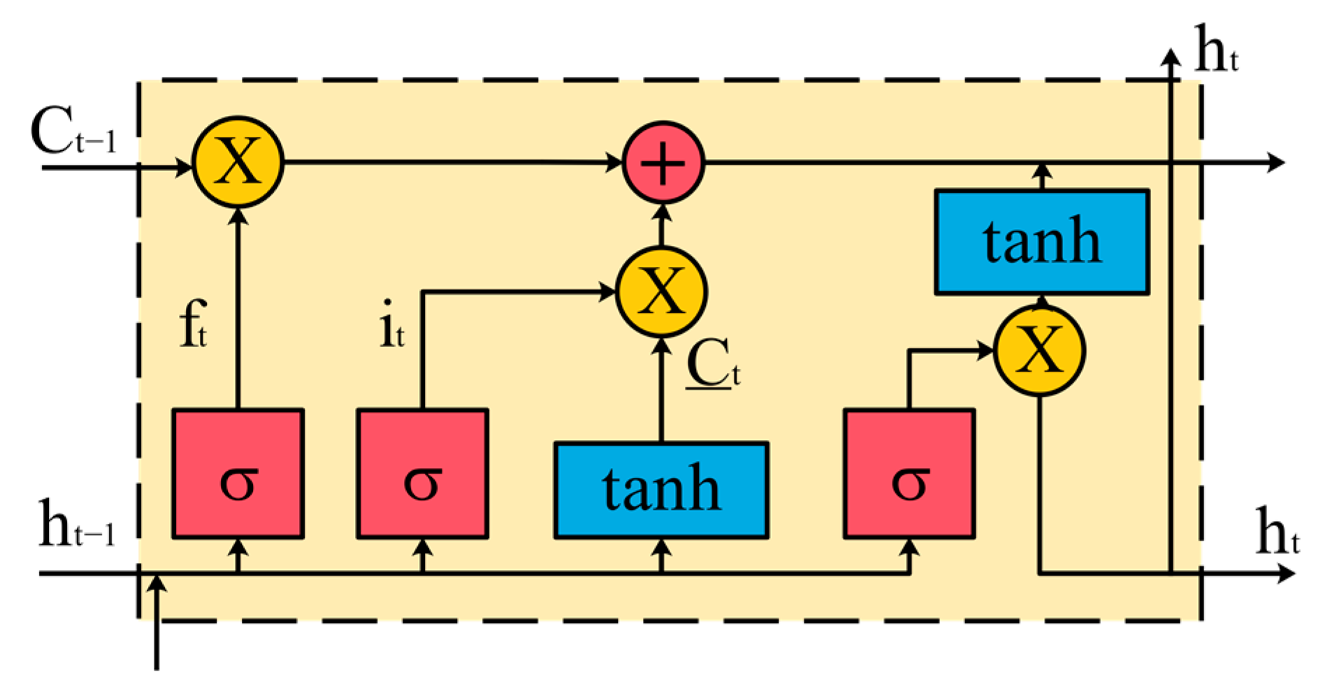
2.1. Long Short-Term Memory (LSTM)

As an improved Recurrent Neural Network (RNN), long short-term memory (LSTM) inherits the advantages of the RNN model and effectively solves the problem of gradient explosion and gradient disappearance in the RNN by using the unique structure of gates [40].

The LSTM consists of multiple cyclic cells, the inputs of which contain the input data at the current moment, the state vector of cyber cells at the previous moment and the hidden layer output vector. LSTM first calculates the discarded information of the cell through the forgetting gate, as shown in Equation (1).

$$f_t=\sigma \left(W_f\cdot \left[h_{t-1},X_t\right]+b_f\right)$$

(1)

where, $W_f$ is the weight matrix of the forgetting gate; into a longer vector; $\left[h_{t-1},X_t\right]$ means connecting two vectors into a longer vector; $b_f$ is the offset term; $f_t$ is the output of the forgetting gate.

The forgetting gate reads $X_t$ and $h_{t-1}$, the size of the output value represents the degree of forgetting and assigns a value to the cell state $C_{t-1}$. The size of $f_t$ is between [0, 1]. The smaller the value is, the higher the degree of forgetting is.

The input gate is partially obtained from the input $X_t$ and $h_{t-1}$ to obtain the current $i_t$, which generates the updated neuron state information $C_t$. The current state information $h_t$ is also calculated from the inputs $X_t$ and $h_{t-1}$ [41]. The input gate is calculated following Equation (2).

$$\{\begin{array}{c}{i}_t=\sigma \left(W_i\cdot \left[h_{t-1},X_t\right]+b_i\right)\\ \widetilde{C_t}=tanh\left(W_c\cdot \left[h_{t-1},X_t\right]+b_c\right)\\ C_t=f_t{C}_{t-1}+i_t\widetilde{C_t}\end{array}$$

(2)

where $W_i$ and $W_c$ are the weight matrix of the input gate, $b_i$ and $b_c$ are the deviation vectors of the output gates, $\widetilde{C_t}$ is the current input cell state. The network structure diagram of LSTM is shown in Figure 1.

Figure 1 shows the forgetting gates and the input gates going to the output gates after a cell state update. Due to its optimized structure, the LSTM can selectively remember the important information and forget the unimportant information. The gradient vanishing problem of the RNN is improved.

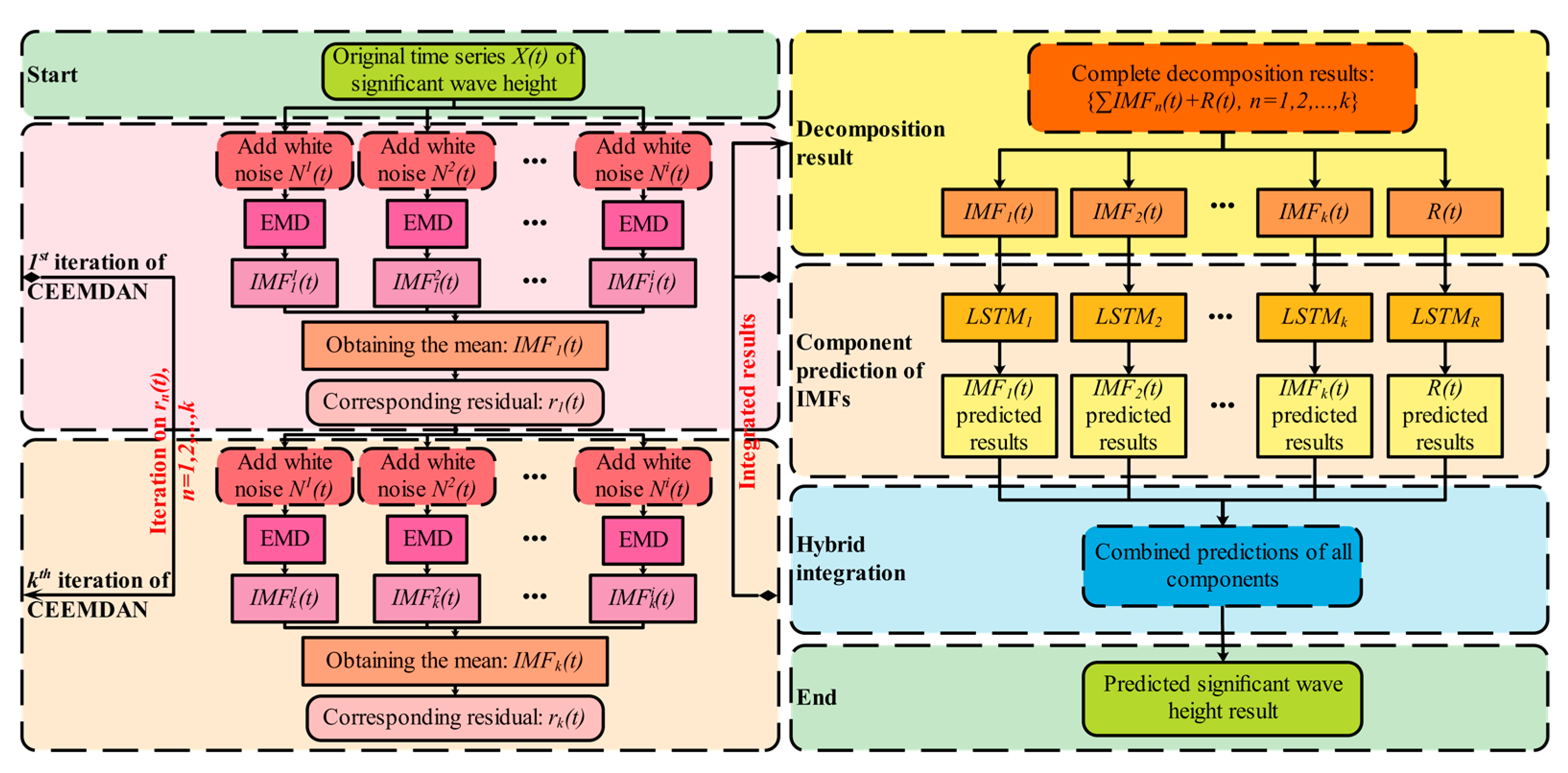
2.2. Complete Ensemble Empirical Mode Decomposition with Adaptive Noise (CEEMDAN)

Huang et al. proposed an empirical mode decomposition (EMD) method for transforming a non-linear sequence into a set of smooth sequences consisting of multiple intrinsic mode functions (IMFs) and a residual [42]. However, the EMD method may lead to mode confounding, and Wu et al. proposed ensemble empirical mode decomposition (EEMD) [43]. The CEEMDAN algorithm obtains the final first-order IMF by performing an average calculation after obtaining the first-order IMF [44]. This operation is repeated for the residual part of the signal, effectively avoiding the transfer of noise from high to low frequencies and overcoming the large reconstruction error in the EEMD algorithm [45,46]. The process of CEEMDAN is described as follows:

• Let $X\left(t\right)$ be the original significant wave height (SWH) of ShiDao effective data, and add white noise $N^i\left(t\right)$ to the load data to form a signal comprising the noise, as shown in Equation (3),

  $$X^i\left(t\right)=X\left(t\right)+X_0{N}^i\left(t\right),i=1,2,\dots ,n$$

  (3)

  where $t$ is various points in time, $i$ represents the $i^{th}$ white noise added to original data, $X_0$ is the standard noise deviation, $N^i\left(t\right)$ is Gaussian white noise, $X^i\left(t\right)$ is the newly generated signal.
• Decompose the $X^i\left(t\right)$ by Equations (4) and (5) to obtain the $1^{st}$ IMF and calculate the corresponding residual $r_1\left(t\right)$.

  $$IM{F}_1\left(t\right)=\frac{1}{n}{{\displaystyle \sum }}_{i=1}^{n}IM{F}_1^i\left(t\right)$$

  (4)

  $$r_1\left(t\right)=X\left(t\right)-IM{F}_1\left(t\right)$$

  (5)
• Gaussian white noise $N^i\left(t\right)$ is added to the residual $r_1\left(t\right)$. The residual expression of adding white noise for the $i^{th}$ time is $r_1^i\left(t\right)=r_1\left(t\right)+N^i\left(t\right)$. The second-order IMF component is determined. EMD decomposes $r_1^i\left(t\right)$ with white noise for the $i^{th}$ time to obtain $IM{F}_2^i\left(t\right)$. The $IM{F}_2\left(t\right)$ is expressed as Equations (6) and (7).

  $$IM{F}_2\left(t\right)=\frac{1}{n}{{\displaystyle \sum }}_{i=1}^{n}IM{F}_2^i\left(t\right)$$

  (6)

  $$r_2\left(t\right)=r_1\left(t\right)-IM{F}_2\left(t\right)$$

  (7)
• Similarly, the $k^{th}$ IMF of CEEMDAN and the $k^{th}$ residual $r_k\left(t\right)$ can be obtained as Equations (8) and (9).

  $$IM{F}_k\left(t\right)=\frac{1}{n}{{\displaystyle \sum }}_{i=1}^{n}IM{F}_k^i\left(t\right)$$

  (8)

  $$r_k\left(t\right)=r_k\left(t\right)-IM{F}_k\left(t\right)$$

  (9)
• The decomposition process will iterate until it reaches a point where the residual is a monotonic function that cannot be decomposed. Whereas $R\left(t\right)$ is the final residual, as shown in Equation (10).

  $$X\left(t\right)={{\displaystyle \sum }}_{n=1}^{k}IM{F}_n\left(t\right)+R\left(t\right)$$

  (10)

2.3. Numerical Algorithms of the Integrated CEEMDAN-LSTM Joint Model

In natural seas, a wave is a time series with non-stationary characteristics and complex irregular non-linear variations. In general, irregular waves are a difficult analytical problem in marine and offshore engineering, and can be numerically solved by computational fluid dynamics (CFD), but they also have the disadvantage of long computational cycles and huge capital expenditure [47].

The combination of CEEMDAN and LSTM models provides an effective method for predicting non-smooth and irregular non-linear waves. The process of wave forecasting using the CEEMDAN-LSTM method is summarized as consisting of three main steps, as shown in Figure 2. The first step is to decompose the wave height time series data with missing values removed into several sets of simple, smooth intrinsic mode functions (IMFs) and residuals based on the CEEMDAN algorithm. The second step is to separately predict each IMF component using the LSTM model. Finally, the predictions for each component are aggregated to obtain the final prediction. The significant wave height forecasts were made based on forecast windows of 1, 3, 6 and 24 h.

2.4. Error Evaluation Indicators

In order to reasonably evaluate the performance of the forecasting model, three metrics, Root Mean Square Error (RMSE), Mean Absolute Error (MAE) and Nash-Sutcliffe Efficiency Coefficient (NSE), are used in this paper to assess the performance of the model. Of these, the RMSE and MAE are more sensitive to the response to errors in very large or very small values in the series, and the NSE provides an assessment of the goodness of fit of the predicted and actual values. The smaller the value of RMSE and MAE, the better the prediction. NSE is between negative infinity and 1, with NSE close to 1 indicating accurate and credible model results; NSE close to 0 indicates that the model results are close to the mean level of the observed values, but with large process errors; and when NSE is much less than 0, the model is not credible.

$$\mathrm{RMSE}=\sqrt{{\frac{1}{n}{{\displaystyle \sum }}_{i=1}^n\left(X_i-X_i^{\prime }\right)}^2},$$

(11)

$$\mathrm{MAE}=\frac{1}{n}{{\displaystyle \sum }}_{i=1}^n\left|X_i-X_i^{\prime }\right|,$$

(12)

$$\mathrm{NSE}=1-\frac{{{\displaystyle \sum }}_{i=1}^n{\left(X_i-X_i^{\prime }\right)}^2}{{{\displaystyle \sum }}_{i=1}^n{\left(X_i-{\overline{X}}_i\right)}^2},$$

(13)

where $X_i$ and $X_i^{\prime }$ are the actual and predicted values of this time series in time period $i$, and $n$ is the number of testing samples.

3. Study Area and Data

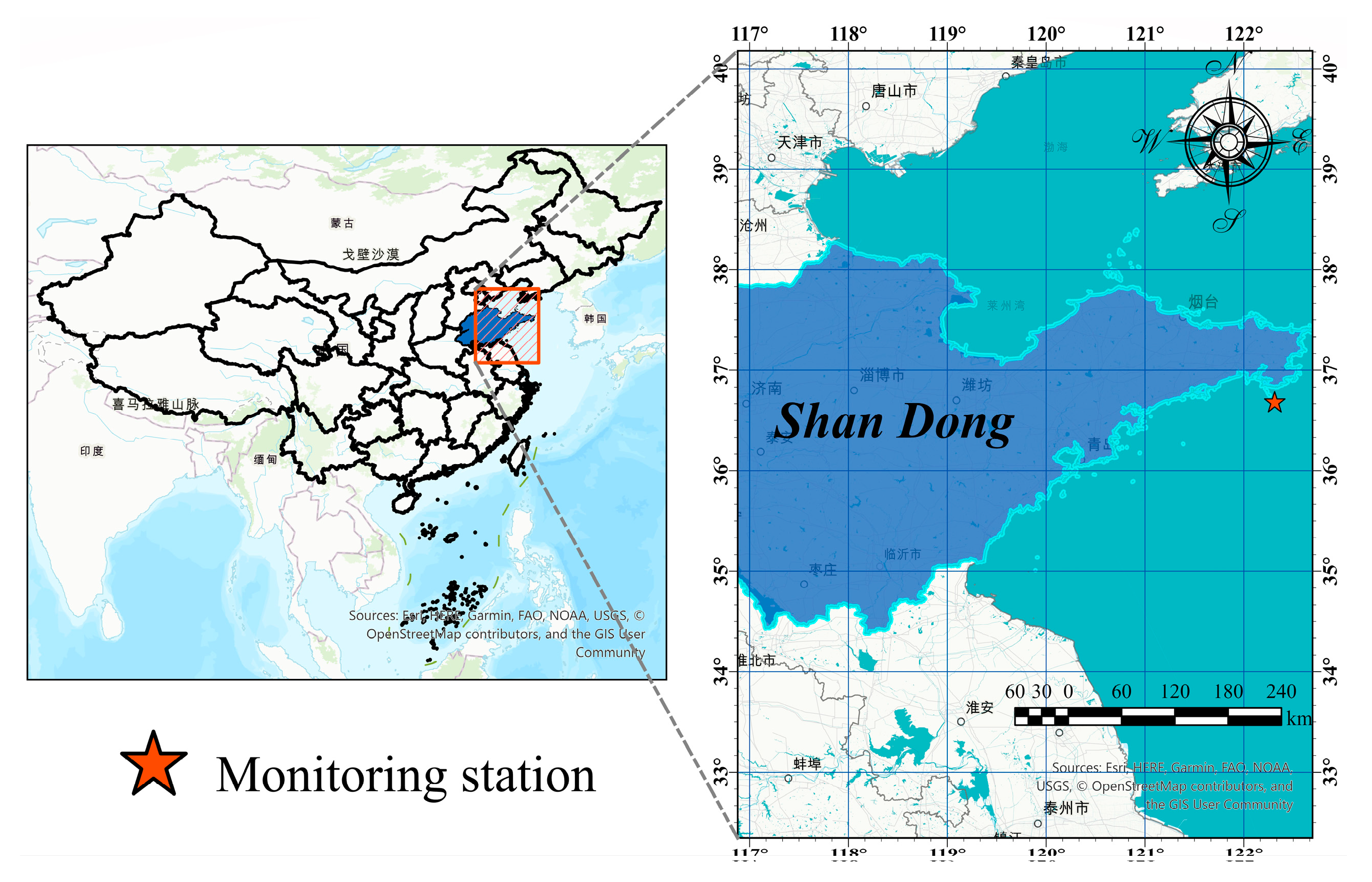
3.1. Description of Study Area

To investigate the wave effects of forecast models with different statistical characteristics, we used the National Marine Data Center, National Science and Technology Resource Sharing Service Platform of China (http://mds.nmdis.org.cn/, accessed on 8 November 2022) to obtain significant wave height (SWH) data from the ShiDao site in Shandong province along the east coast of China. The locations of the east coast of China measured in this paper are shown in Figure 3.

The data from the Shidao site used in this paper covers the period 2013.1.1–2022.7.31, with 73,819 data items. The measured data from the National Marine Data Center, National Science and Technology Resource Sharing Service Platform of China were used. Due to measurement instrumentation and recording bias, we removed missing and extreme outlier values from the data and obtained 68,068 effective data.

Table 1. Spatial location and data statistics.

Monitoring Station	Positon	Data Duration	Dataset	Effective Data
ShiDao	36.89° N 122.43° E	2013.1.1–2022.7.31	73,819	68,068

lists the locations of the measured waves and the data information.

In this paper, the integrated CEEMDAN-LSTM joint model is validated using data from ShiDao monitoring station in this table as input.

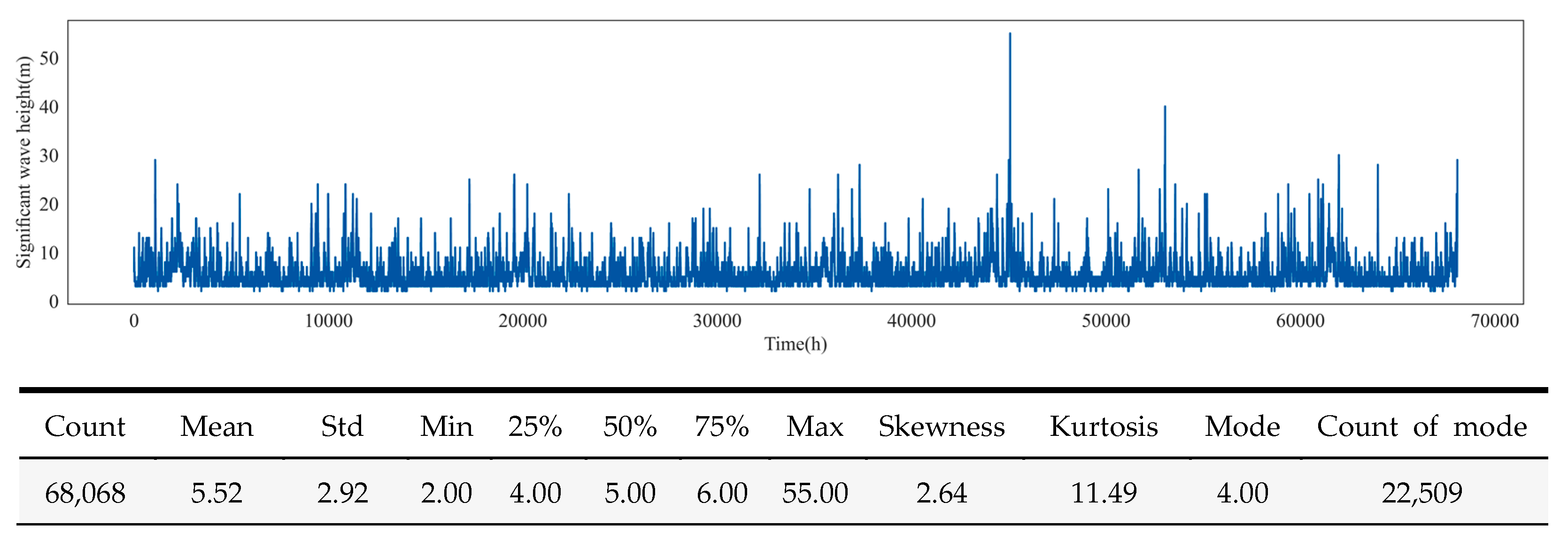
3.2. Significant Wave Height Datasets Preprocessing

The theoretical foundations of both CEEMDAN and LSTM have been established. In order to avoid training errors in the training set being mixed with the test set, which ultimately results in prediction errors. The first 90% of the dataset was classified as the training set and the last 10% was classified as the test set. For the ShiDao dataset, there were 61252 and 6806 data, respectively. Figure 4 shows the time history data and statistical information of significant wave height for ShiDao monitoring station.

As in Figure 4, the mean value of the ShiDao dataset is 5.52, the standard deviation is 2.92 and the mode is 4.00, with a total of 22,509.00 values. The kurtosis value 11.49 is much larger than 3.00, and the probability density distribution curve is sharper and the shape of the peak is steeper than the normal distribution. This indicates, on the one hand, that the distribution of the SWH data has a large number of extreme values. On the other hand, all but the extreme values are concentrated around the mode value of 4.00. The steeper distribution of SWH also poses greater difficulty in terms of prediction. The skewness value is well above 0.00, indicating that the SWH data distribution is positively skewed (right skewed). Consequently, SWH data greater than the mean value of 5.52 accounts for more than half of the data, while the right-hand side of the curve trails off for a long time due to a few outliers being too large.

4. Research Results of the Integration Section

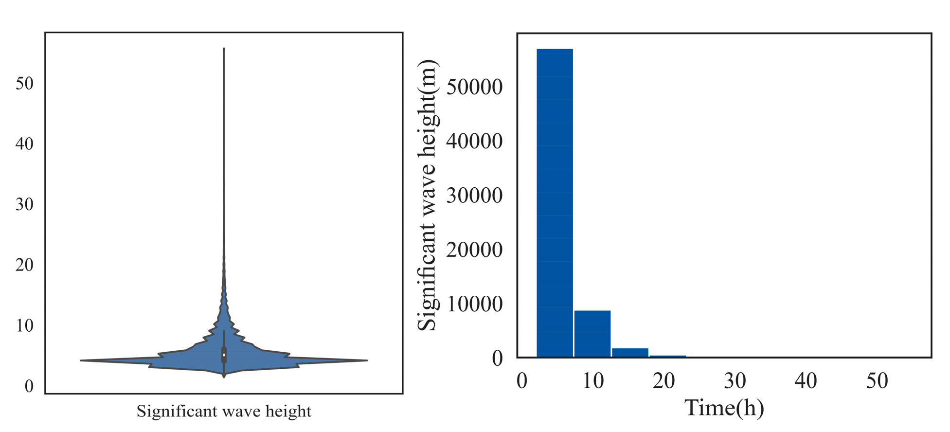
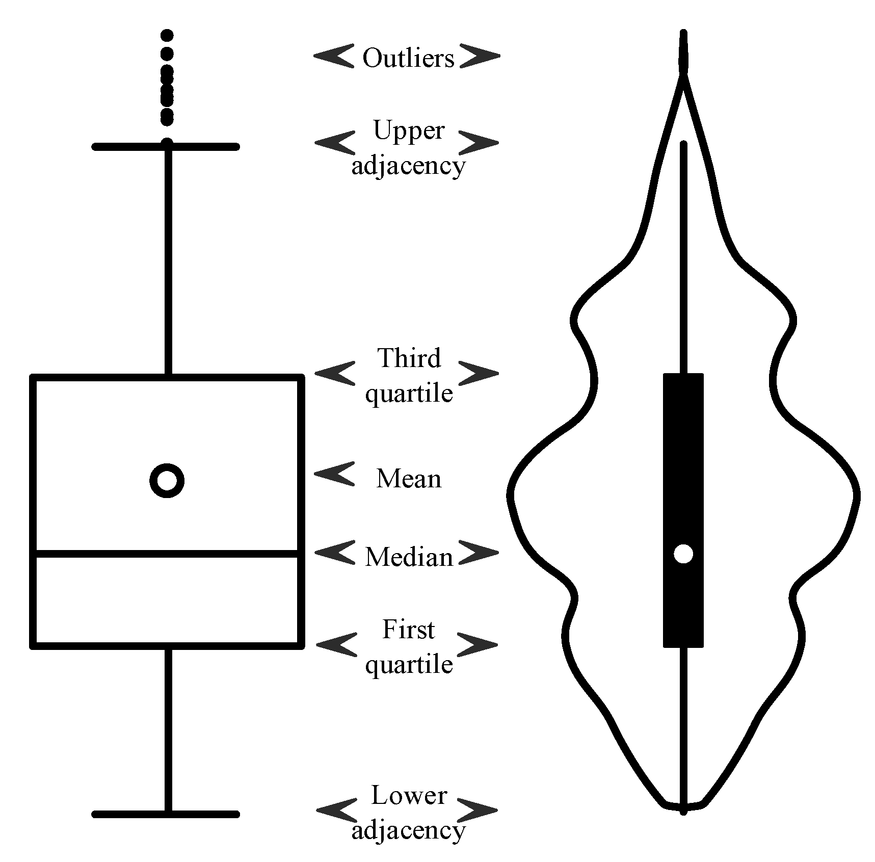
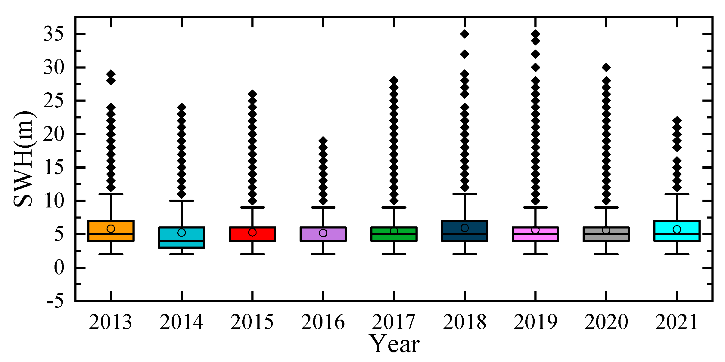
4.1. Novel Filter Formulation for SWH Outliers with Improved Violin-Box Plot

For machine learning and data analysis, the quality of the data is very important. The data in this paper are obtained from actual buoy observations, which are then transmitted in delayed mode and recorded in ASCII character format. As a result, problems such as buoy sensor failures or data transmission errors are inevitable. In order to better characterize the data, a novel filter formulation for SWH outliers is proposed. We first visualized the data using a violin plot and frequency distribution histogram, as shown in Figure 5.

In Figure 5, the violin plot is a combination of a box plot and a kernel density plot, providing us with a way to identify outliers. The white dots on the violin plot represent the median, the thick black bars represent the interquartile range, and the narrow black bars represent the upper and lower adjacencies. Furthermore, the shape of the violin plot shows the overall distribution of the data, which is similar to the results of the frequency distribution histogram. The differences between the specific violin and box plots are shown in Figure 6.

From Figure 6, the violin and box plots give similar information, with the box plot giving additional mean values and the violin plot giving additional information on the distribution of the data. Although normally for machine learning values above the upper and lower adjacency can be considered as outliers and discarded. However, due to the non-linear and non-stationary nature of the SWH data, the volatility is much more dramatic than in normal statistics. The upper bound amplitude is much higher than the upper adjacency of the common statistical range and is real. It is very unjustified to simply discard some data in a crude manner. Therefore, a novel filter formulation for SWH outliers is proposed in this paper by manually checking the measured data from ShiDao monitoring station to remove the missing and extreme outlier values. The box plot of SWH effective data over the years is shown in Figure 7.

The SWH effective data from 2013 to 2021, measured in the field and manually calibrated, is shown in Figure 7. There is no need to assume in advance that the data obey a specific form of distribution. Without any restrictions, the data can be visualized as raw shapes and some common features can be obtained. The data for 2022 is not presented as an effective analysis as it is not yet complete. We can observe that the upper and lower adjacency of the SWH data for all years are around 11 m and 2 m. The mean is around 6 m and the median is less than the mean by about 5 m. The remaining small portion of the data is between 11 m and 35 m. Accordingly, a novel filter formulation for SWH outliers with an improved violin-box plot is proposed to check and modify the SWH outliers, and the procedure is as follows.

$$\{\begin{array}{c}{P}_{25\%}-PD\le y_i\le P_{75\%}+15PD\\ y_i<P_{25\%}-PD\\ y_i>P_{75\%}+25PD\end{array} \begin{array}{c}{Y}_i=y_i\\ Y_i=P_{50\%}-y_{min}\\ Y_i=y_{max}-5P_{50\%}\end{array},$$

(14)

where, $P_{25\%}$, $P_{50\%}$ and $P_{75\%}$ are the 25% quantile, 50% quantile and 75% quantile, respectively, $y_i$ and $Y_i$ are the actual and corrected data, $y_{max}$ and $y_{min}$ are the maximum and minimum values, respectively, and let $PD=P_{75\%}-P_{25\%}$.

The above novel filter formulation works extremely well for positive deviations in SWH data. It may also be applicable for SWH data from other areas of the eastern coast of China. Furthermore, the procedure proposed in the formula is of great interest for other non-linear or non-stationary data.

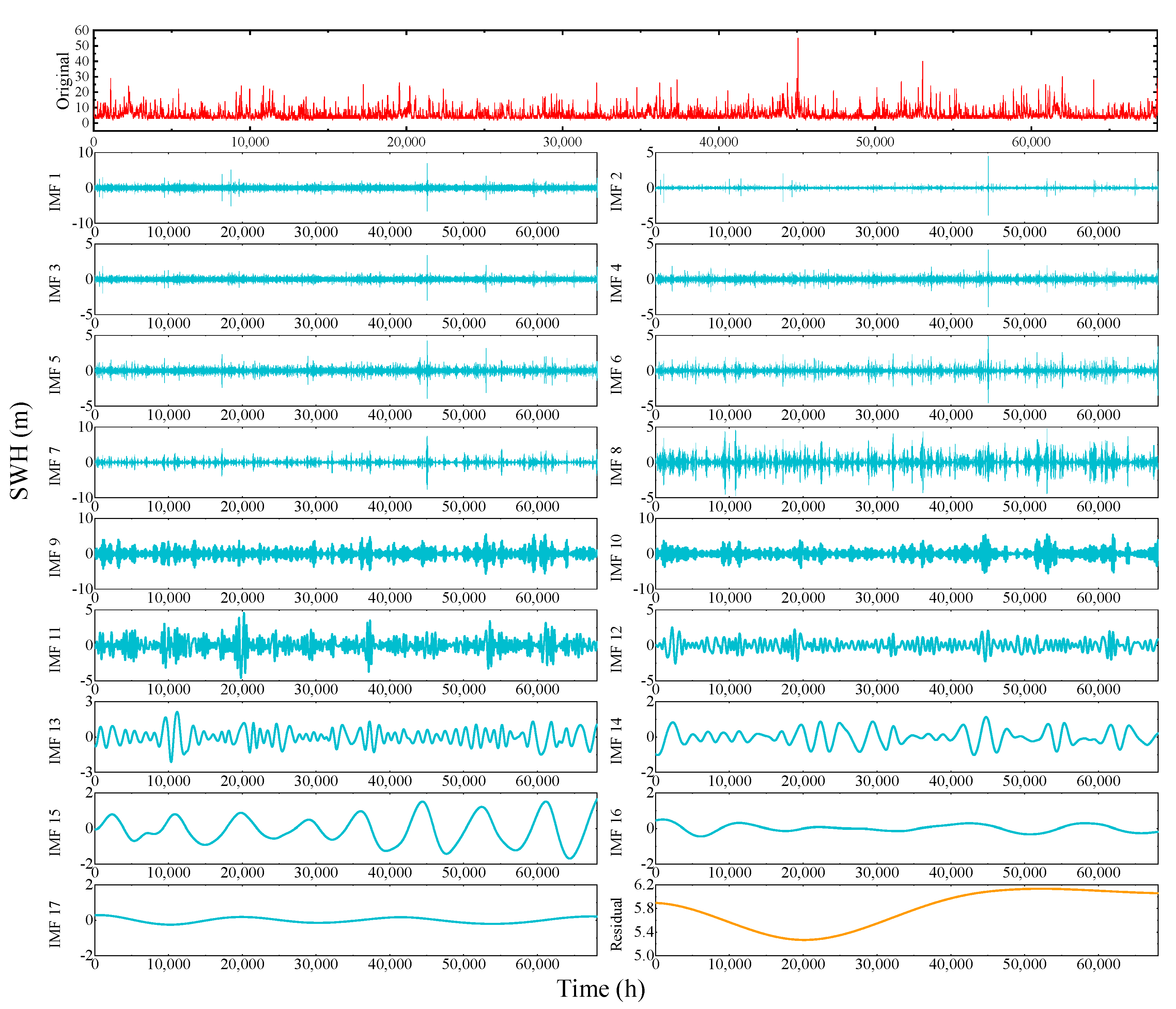
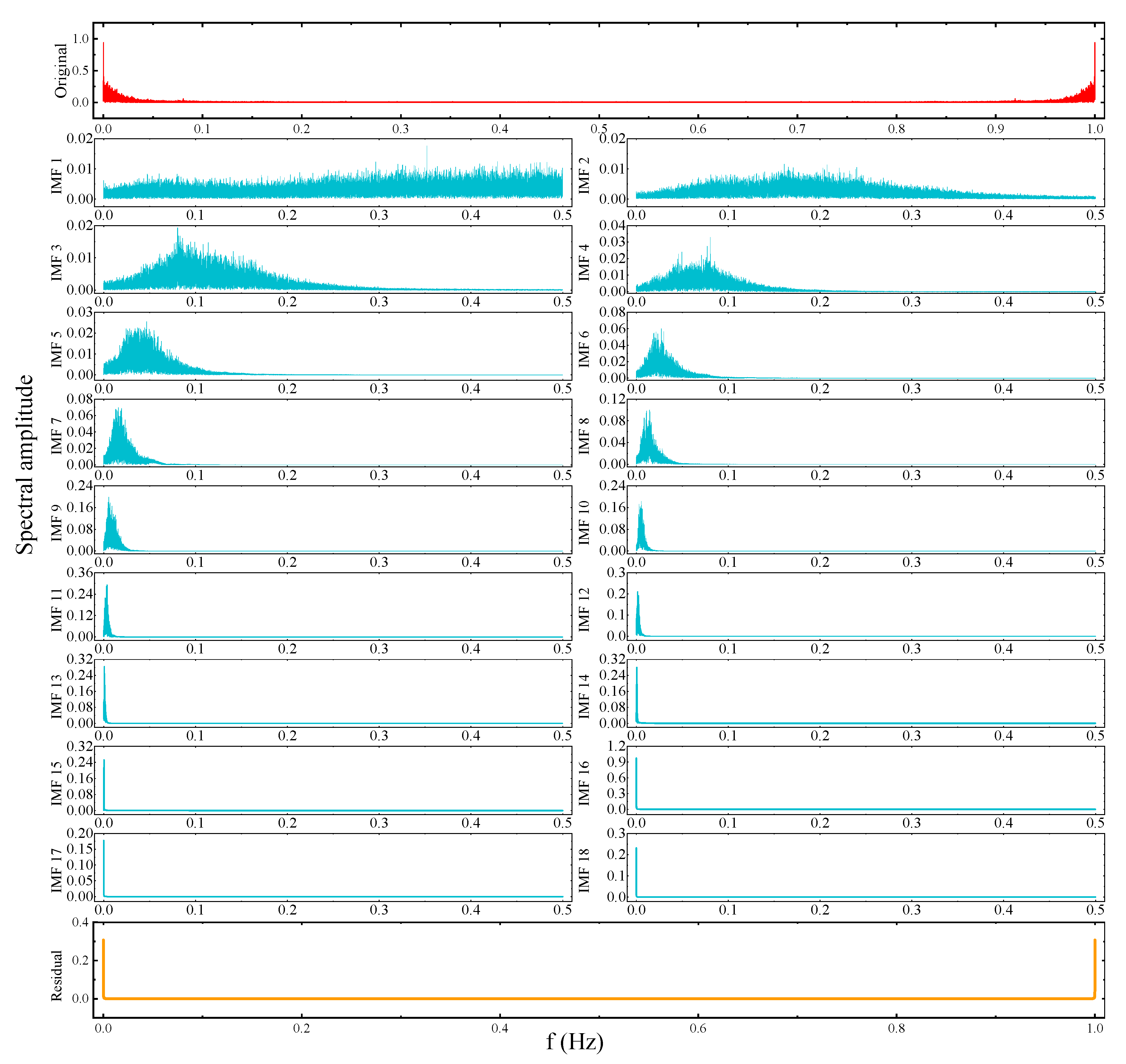
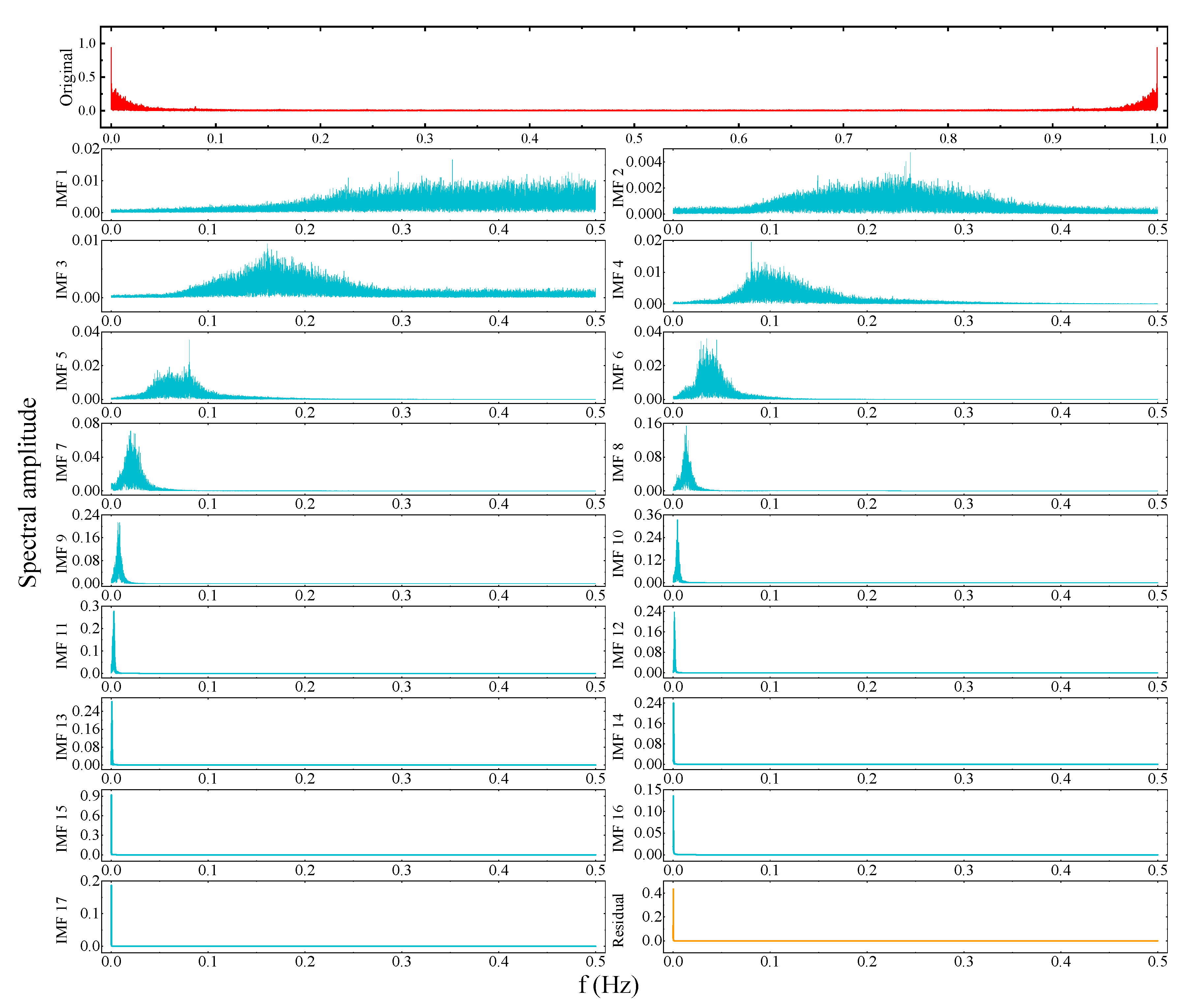
4.2. Decomposition Results of CEEMDAN

The results of the EMD decomposition algorithm are shown in Figure 8. The EEMD and CEEMD decomposition algorithms reduce the modal aliasing of EMD decomposition by adding pairs of positive and negative Gaussian white noise to the signal to be decomposed. However, these two algorithms will always leave a certain amount of white noise in the eigenmode component of the decomposed signal, which affects the subsequent analysis and processing of the signal. The CEEMDAN is an improvement on the EMD and avoids the problem of residual white noise in IMFs of EEMD and CEEMD, as shown in Figure 9.

Figure 8 and Figure 9 show the SWH time history data after processing by EMD and CEEMDAN. There are eighteen IMFs and one residual for EMD and seventeen IMFs and one residual for CEEMDAN. For the ShiDao effective data, we can obtain some conclusions from Figure 8 and Figure 9.

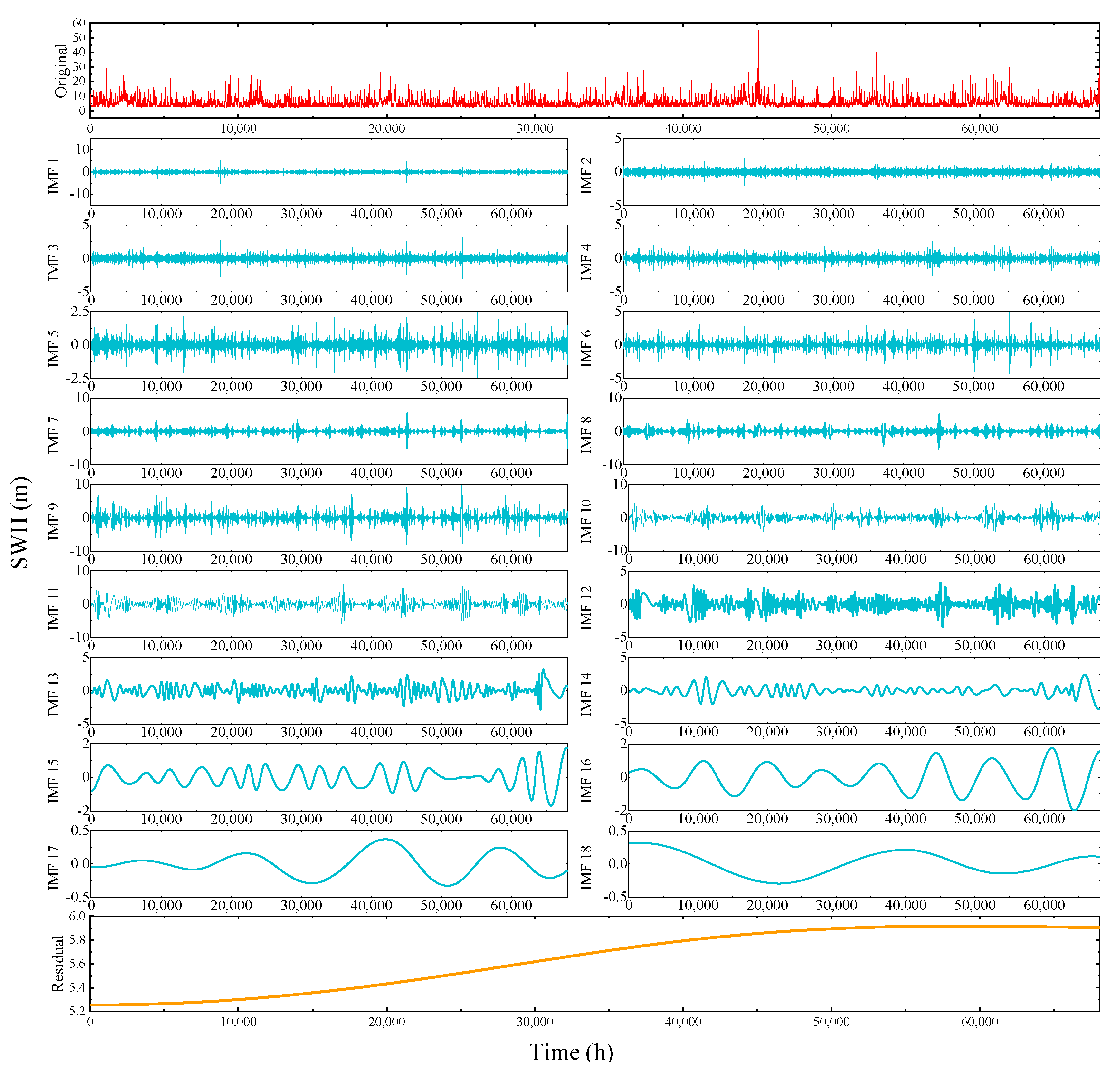
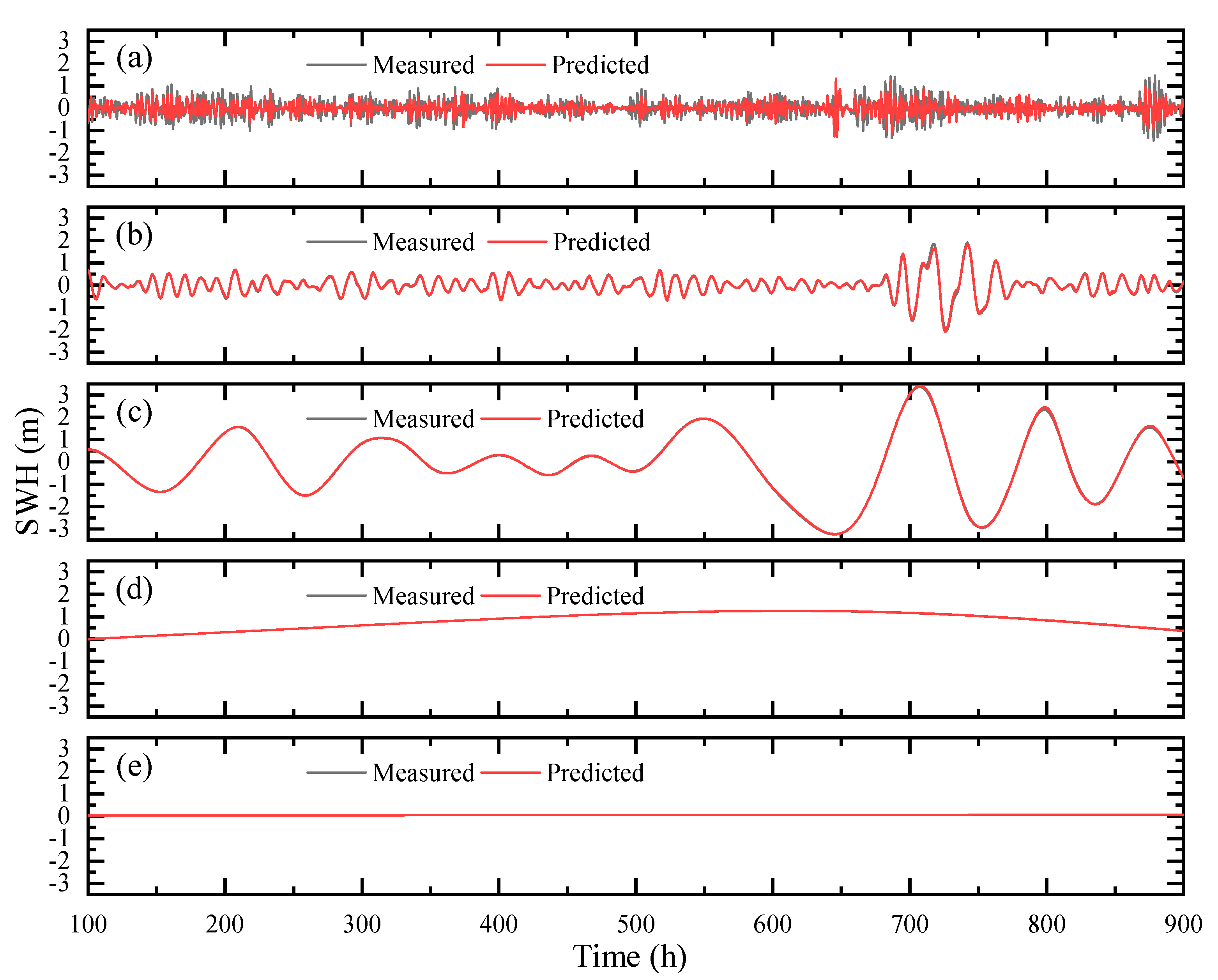
• In Figure 9, the CEEMDAN decomposition of IMF1-IMF7 contains high frequency sinusoidal intermittent signals. IMF8-IMF13 are intermediate frequency sinusoidal intermittent signals. IMF14-IMF17 and the residual are low frequency broad period signals. In this way the signals can be classified. Similarly, the EMD algorithm divides the IMFs components into IMF1-IMF8, IMF9-IMF14 and IMF15-IMF18, respectively.
• From IMF14 onwards, in Figure 9, the signal period increases and gets larger. Local signal surges from a global perspective disappear and the curve becomes increasingly smooth. It can be said that IMF14-IMF17 contain almost no noise at high and medium frequencies. This shows that CEEMDAN has a good processing effect on SWH sequences. A similar phenomenon is observed from IMF15 of EMD onwards. This indicates that CEEMDAN can obtain noise-free IMF components with fewer decomposition steps compared to EMD.
• For the EMD, divergence occurs at the end. For example, IMF13, IMF14 and IMF15 in Figure 8. Whereas, in Figure 9, on the other hand, this does not occur for all IMF components. This indicates that CEEMDAN handles data boundaries much better than EMD. Consider the fact that the upper (lower) envelope of the decomposition process is obtained from the local extremely large (small) values of the signal by three times spline interpolation. However, it is not possible for the endpoints of the signal to be at either a very large or a very small value at the same time. As a result, the upper and lower envelopes diverge at both ends of the data sequence and this divergence gradually increases as the operation proceeds, which is why divergence is a common problem with IMF14-16 in EMD. As the scatter in the decomposition makes the results less scientific, we suspect that this also has a negative impact on the accuracy of the prediction results. However, CEEMDAN does not suffer from such a shortcoming.

The results of the IMFs obtained by EMD and CEEMDAN for the ShiDao effective data in the frequency domain are shown in Figure 10 and Figure 11.

According to Figure 10 and Figure 11, it can be seen that the individual IMFs obtained after EMD and CEEMDAN can be distributed at different frequencies. In Figure 10, we find that the EMD decomposed components show a more pronounced modal mixing: specifically, the peaks of the individual IMF components’ spectra all overlap. This is evident in IMF1-IMF8 in Figure 10. On the contrary, after the CEEMDAN decomposition, it can be seen from Figure 11 that the peaks of all IMF components do not overlap and that all IMF peaks correspond to different frequencies. This shows that the CEEMDAN algorithm can improve and avoid the modal mixing phenomenon in the EMD algorithm. Thus, the original SWH data are decomposed into high frequency sinusoidal intermittent signals, intermediate frequency sinusoidal intermittent signals and low frequency broad period signals.

Consider that the data is monitored in real time on an hourly basis at the ShiDao monitoring station. Therefore, in terms of physical significance:

• The high frequency sinusoidal intermittent signals IMF1-IMF7 can reflect the essential characteristics of SWH data. For example, a tidal cycle (approximately 24 h and 50 min) is accompanied by a high tide and a low tide, which is reflected in one cycle of the high frequency sinusoidal interval signal.
• The intermediate frequency sinusoidal intermittent signals IMF8-IMF13 reflect the medium- and long-term meteorological influences of the monsoon and ocean currents on the SWH data, alternating between weekly and monthly cycles.
• In the modeling and analysis processes, the low frequency signals IMF14-IMF17 can be seen as a very small energy loss of the high frequency intermittent signals.

5. Analysis of Substantiation Results

Although LSTM, as a particular type of RNN, has been widely used for time series prediction due to its powerful ability to selectively remember and forget information. However, LSTM, like all methods, is limited by its mathematical basis and the inability of science to fully observe physical phenomena. Therefore, it is necessary to add other tools. In this paper, we test the LSTM and integrated CEEMDAN-LSTM models with SWH effective data obtained from the ShiDao monitoring station off the east coast of China using the National Marine Data Center, National Science and Technology Resource Sharing Service Platform of China. The first 90% of the dataset was classified as the training set and the last 10% was classified as the test set. For the ShiDao effective dataset, there were 61,252 and 6806 data, respectively. The model uses a rolling mechanism to iteratively predict n future values from the input data (n = 1,3,6,24 corresponding to 1, 3, 6 and 24 h ahead, respectively). The real SWH data from the next iteration step is then used as the known input to the model to continue the prediction with a rolling forecast. Due to the large amount of data, overfitting is less likely to occur. However, in order to increase the applicability of the model and further reduce the possibility of overfitting, a dropout layer was set up with 50% random discarding used to prevent overfitting [48].

5.1. Summary of Model Parameter Settings

In order to make the article scientifically sound and reproducible, we list the parameters of the CEEMDAN-LSTM. For the CEEMDAN algorithm: the sampling frequency is set to 1, the standard deviation of the additional Gaussian noise is set to 0.2, the number of times the signal is averaged is 100 and the maximum number of iterations is set to 1000.

The prediction accuracy of a neural network can be improved by adding more layers or more neurons. However, in some cases, adding more layers and neurons is not conducive to improving the accuracy of a neural network while increasing the training time. In this study, the number of layers of hidden neurons in the LSTM network structure model was set to 2. The first layer of the LSTM hidden layer contained 200 neurons and the second layer contained 100 neurons. The hidden layer of the first LSTM outputs $h_t$, which is passed as input to the second LSTM layer, and into the hidden layer of the second LSTM layer. This is followed by a dropout, where 50% of the neural network units are randomly discarded to prevent overfitting. Finally, there is a fully connected layer with only one neuron, and the output size of the fully connected layer is equal to the size of the prediction result. The regression layer computes the half-mean-square-error loss to check the convergence of the network.

The model was implemented using the MATLAB Deep Learning Toolbox. In this network, training was performed based on the adaptive moment estimation (Adam) optimizer. For the three datasets in this paper, the number of iterations of the maximum Epochs is 500 and the mini Batch Size is 16. The initial learn rate, learn rate drop factor and learn rate drop period were 0.005, 0.2 and 100, respectively, with a piecewise learn rate schedule.

5.2. Error Evaluation Indicators Quantify the Degree of Improvement

Using the error evaluation indicators in Equations (11)–(13), we were able to quantify the improvement of CEEMDAN-LSTM over LSTM.

Table 2. Comparison of ShiDao measured and predicted values by error evaluation indicators between CEEMDAN-LSTM and LSTM with degree of improvement for the 1-, 3-, 6- and 24-h forecast windows.

Forecast Durations (h)	LSTM			CEEMDAN-LSTM			Degree of Improvement
	RMSE (m)	MAE (m)	NSE	RMSE (m)	MAE (m)	NSE	RMSE (%)	MAE (%)	NSE (%)
1	0.7693	0.1096	0.9312	0.2162	0.0346	0.9946	71.90%	68.46%	6.80%
3	0.8297	0.1154	0.9234	0.2693	0.0430	0.9916	68.75%	62.70%	7.39%
6	0.8940	0.1206	0.9167	0.3225	0.0515	0.9879	66.17%	57.29%	7.76%
24	0.9720	0.1290	0.9016	0.4825	0.0770	0.9729	53.44%	40.31%	7.91%

presents the results of the error evaluation indicators analysis to determine the effectiveness of LSTM and CEEMDAN-LSTM for 1-, 3-, 6- and 24-h forecast windows.

By expanding the prediction window, it can be easily observed from Table 2: The RMSE and MAE of both LSTM and CEEMDAN-LSTM are steadily increasing, while the NSE is decreasing. This all indicates that model performance gradually decreases as the forecast duration increases. However, using any of RMSE, MAE or NSE to measure the performance of CEEMDAN-LSTM is significantly higher than the predictions of LSTM at each forecast duration. The extent of the improvement of CEEMDAN-LSTM over LSTM clearly demonstrates that over increasingly longer time scales, the integrated CEEMDAN-LSTM joint model is able to slow down error growth and maintain a good correlation with the observations. At 1 h, the error evaluation indicators showed the most significant increase, corresponding to 71.90% for RMSE, 68.46% for MAE and 6.80% for NSE. Even with a 24-h advance, CEEMDAN-LSTM still improves by 53.44%, 40.31% and 7.91% over LSTM in terms of RMSE, MAE and NSE. Consequently, the impact of CEEMDAN-LSTM on the results of short-term forecasts is significant.

5.3. Statistical Tests of Prediction Results

The Friedman test [49] and post hoc Nemenyi test [50] were added to ensure the rationality of the results. The Friedman test is a non-parametric test of whether there are significant differences between multiple overall distributions using rank. The main hypothesis of the principle is that there is no significant difference in the distribution of multiple populations from multiple pairing samples [51]. Before performing the Friedman test, the data was first tested for normal distribution. Due to the large volume of data, the Kolmogorov-Smirnov test was used. If the data did not conform to a normal distribution, then the Friedman test could be used; otherwise the ANOVA was used. The post hoc Nemenyi test could be followed up with multiple comparisons.

After testing, the sample N were greater than 5000 using the K-S test, the significance p-value was 0.001, which presented significance at the level and rejected the original hypothesis. Therefore,

Table 3. The Friedman test results using LSTM.

Serial Number	Variable Name	Sample Size	Median	Standard Deviation	Statistical Quantities	p	Cohen’s f Value
①	Measurement	6806	5.000	2.934	6967.366	0.001	0.020
②	Prediction (1 h)	6806	4.679	2.833
③	Prediction (3 h)	6806	4.645	2.824
④	Prediction (6 h)	6806	4.491	2.788
⑤	Prediction (24 h)	6806	4.541	2.711

,

Table 4. The post hoc Nemenyi test using LSTM for multiple comparisons.

Pairing Variables	Median ± Standard Deviation			Statistical Quantities	p	Cohen’s d
	Pairing 1	Pairing 2	Pairing Difference (Pairing 1–Pairing 2)
① pairing ②	5.000 ± 2.934	4.679 ± 2.833	0.321 ± 0.101	51.686	0.001	0.015
① pairing ③	5.000 ± 2.934	4.645 ± 2.824	0.355 ± 0.109	25.375	0.001	0.009
① pairing ④	5.000 ± 2.934	4.491 ± 2.788	0.509 ± 0.146	60.732	0.001	0.041
① pairing ⑤	5.000 ± 2.934	4.541 ± 2.711	0.459 ± 0.223	10.234	0.001	0.010
② pairing ③	4.679 ± 2.833	4.645 ± 2.824	0.034 ± 0.009	26.311	0.001	0.007
② pairing ④	4.679 ± 2.833	4.491 ± 2.788	0.188 ± 0.045	112.418	0.001	0.058
② pairing ⑤	4.679 ± 2.833	4.541 ± 2.711	0.138 ± 0.123	41.452	0.001	0.026
③ pairing ④	4.645 ± 2.824	4.491 ± 2.788	0.154 ± 0.036	86.108	0.001	0.051
③ pairing ⑤	4.645 ± 2.824	4.541 ± 2.711	0.104 ± 0.114	15.141	0.001	0.020
④ pairing ⑤	4.491 ± 2.788	4.541 ± 2.711	0.050 ± 0.078	70.967	0.001	0.033

where Cohen’s d value indicates the effect size. 0.20 or below indicates a small effect, 0.20 to 0.50 indicates a small effect, 0.50 to 0.80 indicates a large effect, and 0.80 or above indicates a large effect.

,

Table 5. The Friedman test results using CEEMDAN-LSTM.

Serial Number	Variable Name	Sample Size	Median	Standard Deviation	Statistical Quantities	p	Cohen’s f Value
①	Measurement	6806	5.000	2.934	6.223	0.183	0.001
②	Prediction (1 h)	6806	4.752	2.922
③	Prediction (3 h)	6806	4.694	2.921
④	Prediction (6 h)	6806	4.65	2.921
⑤	Prediction (24 h)	6806	4.627	2.926

and

Table 6. The post hoc Nemenyi test using CEEMDAN-LSTM for multiple comparisons.

Pairing Variables	Median ± Standard Deviation			Statistical Quantities	p	Cohen’s d
	Pairing 1	Pairing 2	Pairing Difference (Pairing 1–Pairing 2)
① pairing ②	5.000 ± 2.934	4.752 ± 2.922	0.248 ± 0.012	2.775	0.285	0.002
① pairing ③	5.000 ± 2.934	4.694 ± 2.921	0.306 ± 0.013	2.775	0.285	0.002
① pairing ④	5.000 ± 2.934	4.650 ± 2.921	0.350 ± 0.013	2.821	0.268	0.002
① pairing ⑤	5.000 ± 2.934	4.627 ± 2.926	0.373 ± 0.008	2.783	0.282	0.002
② pairing ③	4.752 ± 2.922	4.694 ± 2.921	0.058 ± 0.001	0.000	0.900	0.000
② pairing ④	4.752 ± 2.922	4.650 ± 2.921	0.102 ± 0.001	0.046	0.900	0.000
② pairing ⑤	4.752 ± 2.922	4.627 ± 2.926	0.125 ± 0.004	0.008	0.900	0.000
③ pairing ④	4.694 ± 2.921	4.650 ± 2.921	0.044 ± 0.000	0.046	0.900	0.000
③ pairing ⑤	4.694 ± 2.921	4.627 ± 2.926	0.067 ± 0.005	0.008	0.900	0.000
④ pairing ⑤	4.650 ± 2.921	4.627 ± 2.926	0.023 ± 0.005	0.038	0.900	0.000

show the results of the mathematical statistics tests, the data did satisfy the normal distribution and could be subjected to the Friedman test, the results of which are shown in Table 3 and Table 5. Then, the post hoc Nemenyi test was used to carry out two-by-two multiple comparisons, the results of which are shown in Table 4 and Table 6.

The results of the Friedman test include the median, statistic and Cohen’s f-value. When the p-value is significant (p < 0.05), the original hypothesis is rejected, indicating that there is a significant difference between the two sets of data and that the difference can be analyzed on the basis of median ± standard deviation, and vice versa, indicating that the data do not show variability. Cohen’s f-value was used to indicate the effect size, with the threshold for differentiation of small, medium and large effect sizes being: 0.1, 0.25 and 0.40, respectively.

The table of results analyzed using Friedman’s test shows that the significant p-value is 0.001. Therefore, the statistical result is significant, indicating that there is a significant difference between the individual Variable names. The magnitude of the difference Cohen’s f value was: 0.02, a very small degree of difference.

The post hoc Nemenyi test was used to compare two variables, and all the results showed a p-value of 0.001, showing significance at the level and rejecting the original hypothesis; therefore, there is a significant difference between the two variables. For CEEMDAN-LSTM, the same test procedure as above was used.

The results of the Friedman test analysis showed that the significant p-value was 0.183, and therefore, the statistical results were not significant. It means that there is no significant difference between Measurement, Prediction (1 h), Prediction (3 h), Prediction (6 h) and Prediction (24 h). The magnitude of the difference Cohen’s f value was: 0.001, a very small degree difference.

The post hoc Nemenyi test was used to compare two variables. From Table 6, it can be seen that the significance p-values are 0.285, 0.268,0.282 and 0.900, which present insignificance at the level. The original hypothesis cannot be rejected, and therefore, there is no significant difference between the two variables. From the results of the Friedman test and post hoc Nemenyi test, the LSTM prediction results were tested to be significant at the p-value level, while the CEEMDAN-LSTM prediction results were tested to be non-significant at the p-value level. This indicates that CEEMDAN-LSTM significantly improved the prediction performance.

5.4. Analysis of Substantiation Results through Data Visualization

A fixed sliding data window with a sample size of 800 h SWH records was designed as the model identification sample, and the corresponding 800 h data was taken for experimental validation. The results are realistic in Figure 12, the effectiveness of LSTM-based and CEEMDAN-LSTM predictions of SWH for 1-, 3-, 6- and 24-h windows can be examined.

From Figure 12, it is easy to see that CEEMDAN-LSTM predicts the change in SWH trend significantly better than LSTM. The difference in prediction accuracy between the two methods was small at 1 h of prediction, and it was not easy to distinguish between the two as being clearly superior or inferior. However, the prediction errors of the LSTM sharply accumulated over time, as observed in the later forecast durations. For example, in Figure 12b–d, the forecast durations are set to 3, 6 and 24 h. The LSTM and CEEMDAN-LSTM forecasts are progressively inconsistent with the observations, and the forecasts become progressively worse. The deviation in the LSTM predictions (blue line) from the measured values can be clearly seen in Figure 12d. This is particularly true in the case of large SWH measured values; for example, for peaks around 700 h.

Therefore, we have zoomed in on the 640-h to 760-h window. The advantages of the CEEMDAN-LSTM can be seen more clearly in Figure 12e–h. The CEEMDAN-LSTM (red line) tries to fit the local oscillations in the SWH measured values around 640 h, whereas the LSTM (blue line) is fitted with a smooth curve averaging the amplitude of the oscillation region. Thus, we believe that the CEEMDAN-LSTM responds more aggressively to local oscillatory mutations and that the LSTM does not try to fit such oscillations. Hence, the CEEMDAN-LSTM is clearly the best at predicting the 3 h in Figure 12e. As the forecast duration increases, the CEEMDAN-LSTM results are larger in magnitude compared to the measured values, while the LSTM continues to make no effort to fit any oscillations. A similar phenomenon is observed for the peak at 710 h.

All of the above demonstrates that the LSTM itself cannot accurately predict SWH values. However, the CEEMDAN-LSTM is better adapted to the prediction of extreme value points when the SWH is rapidly changing.

In order to compare the prediction effectiveness of the two methods more objectively, the prediction error histogram is shown in Figure 13. Errors larger than 4 m are grouped together, while errors smaller than −4 m are grouped together, and the total frequency of each occurrence (the number of occurrences of an error of a particular magnitude) is shown.

As the forecast duration progresses (as shown in Figure 13a–d, where forecast errors are given for 1-, 3-, 6- and 24-h windows in turn), the forecast errors for both methods gradually increase. The error distribution of the LSTM shows a normal distribution, although these errors are generally concentrated between ±2 m and especially between ±0.5 m. However, it is clear that the frequency of ±0.5 m errors also decreases with time. This implies that the LSTM prediction effect rapidly diminishes with forecast duration. Unlike the normal distribution of LSTM, the distribution of CEEMDAN-LSTM forecast errors is more concentrated and is around ±0.5 m in Figure 13a–c. The number of CEEMDAN-LSTM errors greater than ±0.5 m under a Figure 13d forecast duration of 24 h is also much smaller than that of LSTM. This shows that the integrated CEEMDAN-LSTM joint model not only has a significantly higher prediction accuracy than the LSTM, but also performs better in terms of the distribution of cumulative errors.

The measured and predicted values in the high, intermediate and low frequency IMFs are depicted in Figure 14. For reasons pertaining to space, only five IMFs are plotted.

It can be seen from Figure 14a that the prediction of the high frequency (HF) component IMF1 is slightly worse, but the subsequent intermediate and low frequency components are almost in line with the measured value, as in Figure 14b–e. However, the fact that the predicted values of IMF1 also capture the main trend of the measured value is an important reason why CEEMDAN-LSTM has better prediction results compared to LSTM. Comparing the negative fit of the LSTM model to the fluctuating trend of the data in Figure 12e–h, the CEEMDAN-LSTM handles the situation much better. Therefore, it can be concluded that the CEEMDAN-LSTM model can significantly improve prediction quality. The main reason for this is that the LSTM is unable to capture HF signals, but after CEEMDAN decomposes a given signal into IMFs components, the underlying trend of the data can be separated from the HF signal in the form of intermediate and low frequencies, thus significantly improving the predictive power. In the case of HF IMFs, studies have shown that they may contain wind direction and speed information. Further research on HF signals may therefore improve the accuracy of SWH forecasts [52,53]. This provides a direction for improving the interpretability of the integrated CEEMDAN-LSTM joint model and for further improvements.

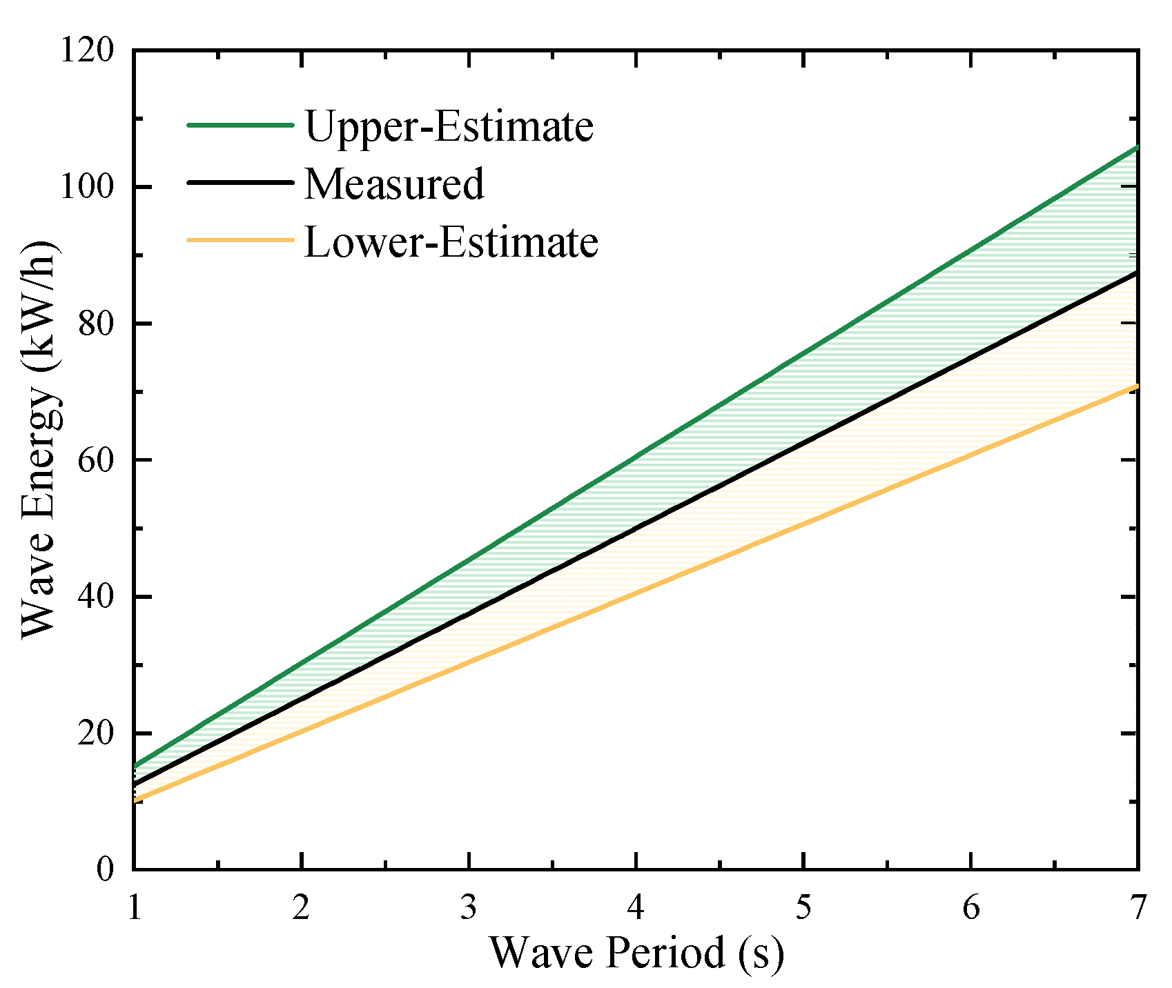
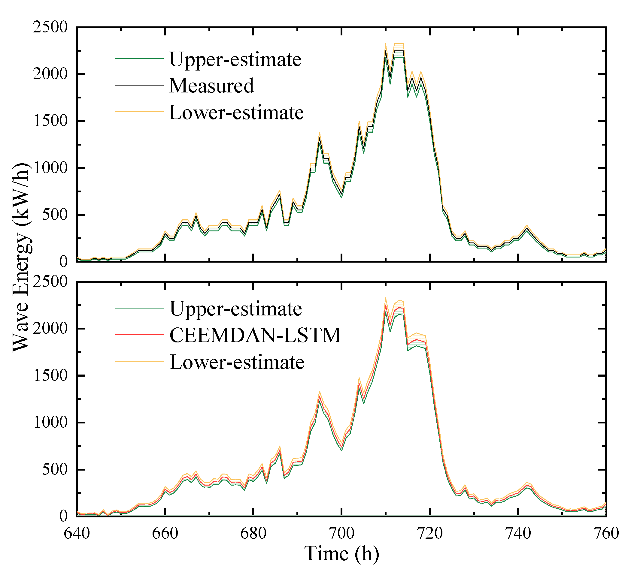
5.5. Performance of SWH Predictions on Wave Energy

As an important source of clean energy, wave energy estimation has considerable sensitivity to SWH (which is $W\propto H_s^2·\mathrm{Tp}$) [54]. Here, the predictions of the integrated CEEMDAN-LSTM joint model can be substituted into $H_s^2$ to estimate wave energy. Slight deviations in the resulting predictions have a corresponding two times the deviation from the total energy estimate. As the CEEMDAN-LSTM outperforms the LSTM for the 1-, 3-, 6- and 24-h cases, and has an outstanding prediction performance for the 1-h forecast duration, its accurate prediction is crucial for the development and commercial viability of wave energy conversion as a clean energy source.

Figure 15 provides an example of a wave energy estimate. Here, the SWH measured values (black) are 5 m, the wave period is 2–6 s and the upper-estimate and lower-estimate offsets are about 0.5 m.

It can be seen from Figure 15 that, for a wave period of 1 m, the estimated wave energy is between 10 and 15 kW/m. Similarly, for a wave period of 2 m, the estimated wave energy is between 20 and 30 kW/m. Applying a similar example from Figure 15 to the predicted results of the integrated CEEMDAN-LSTM joint model, wave energy estimates can be made from our model. The results of wave energy estimation by CEEMDAN-LSTM for the Figure 12e–h subplot time window (640–760 h) are plotted against the measured values in Figure 16 here so that the wave period is 5 s. It can be seen that the wave energy obtained from the CEEMDAN-LSTM prediction of the SWH prediction is almost identical to that obtained from the measured values, especially in the 710-h peak region. This proves that it is feasible to use the results of the integrated CEEMDAN-LSTM joint model for wave energy estimation.

6. Comparison with the Work of Peers

We believe that comparison with peer work is important, and therefore, here we have chosen two models to compare with our CEEMDAN-LSTM, MFRFNN [55] and VMD-MFRFNN [56]. We chose to uniformly use the RMSE at 1 h ahead to evaluate the performance of the models. The results are shown in

Table 7. Comparison of the performance of CEEMDAN-LSTM with other models.

Source	Model	Forecast Durations (h)	RMSE (m)
The research work of Nasiri and Ebadzadeh	MFRFNN	1	0.5493
	VMD-MFRFNN	1	0.2182
Our research work	LSTM	1	0.7693
	CEEMDAN-LSTM	1	0.2163

.

Table 7 shows that the performance of MFRFNN is superior to that of the traditional LSTM. The two integrated algorithms, VMD-MFRFNN and CEEMDAN-LSTM, are very similar in performance. The CEEMDAN-LSTM proposed in our study is slightly better. Given that both MFRFNN and VMD-MFRFNN are very high performing prediction algorithms, we can conclude that the integrated CEEMDAN-LSTM joint model still performs reasonably well compared to the advanced prediction models. Therefore, CEEMDAN-LSTM has important implications for SWH forecasting.

7. Conclusions

The prediction of SWH is crucial for the development and exploitation of marine energy, the construction and maintenance of marine projects and maritime activities. Making accurate SWH forecasts is not only a challenging problem for predicting nonlinear and nonstationary series, but it is also highly relevant to the development of marine energy and the conduct of marine engineering and maritime activities. It is for this reason that an equally wide range of physically based numerical fluctuation and statistical models have been developed to implement short- and long-term SWH predictions. In this paper, we developed an integrated CEEMDAN-LSTM joint model to improve the predictions of the single LSTM model by comparing it with the SWH model, in terms of the symbiotic relationship between CEEMDAN and LSTM networks and the different responses to data fitting. This was used to improve the single LSTM model predictions. The contributions of this research paper are as follows.

• This paper proposes a novel filter formulation for SWH outliers based on an improved violin-box plot, which is able to filter SWH data with positive skewed distribution. It may also be applicable to SWH data from other regions along the eastern coast of China. In addition, the process proposed in this formulation is also of great interest for other nonlinear or nonstationary data.
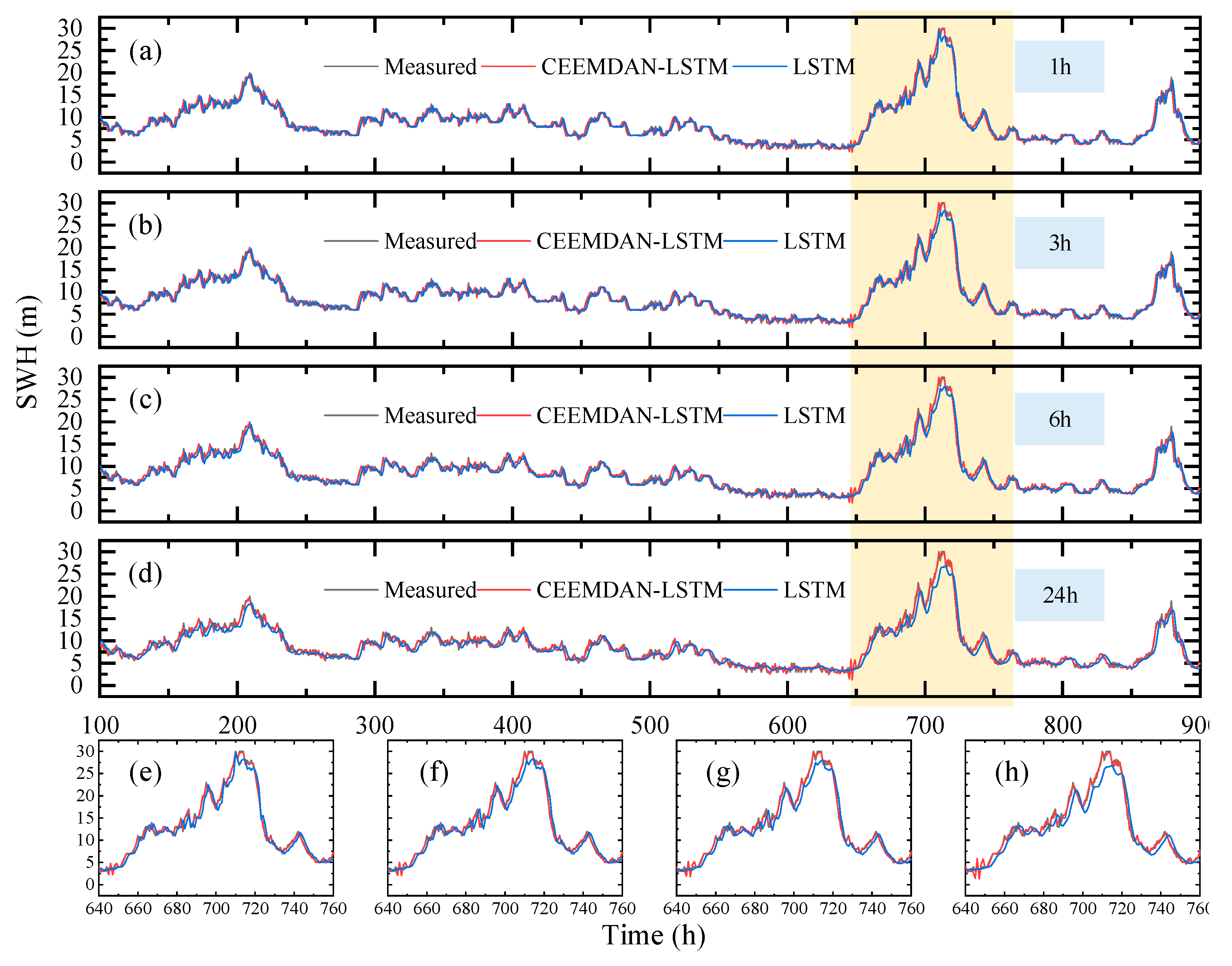
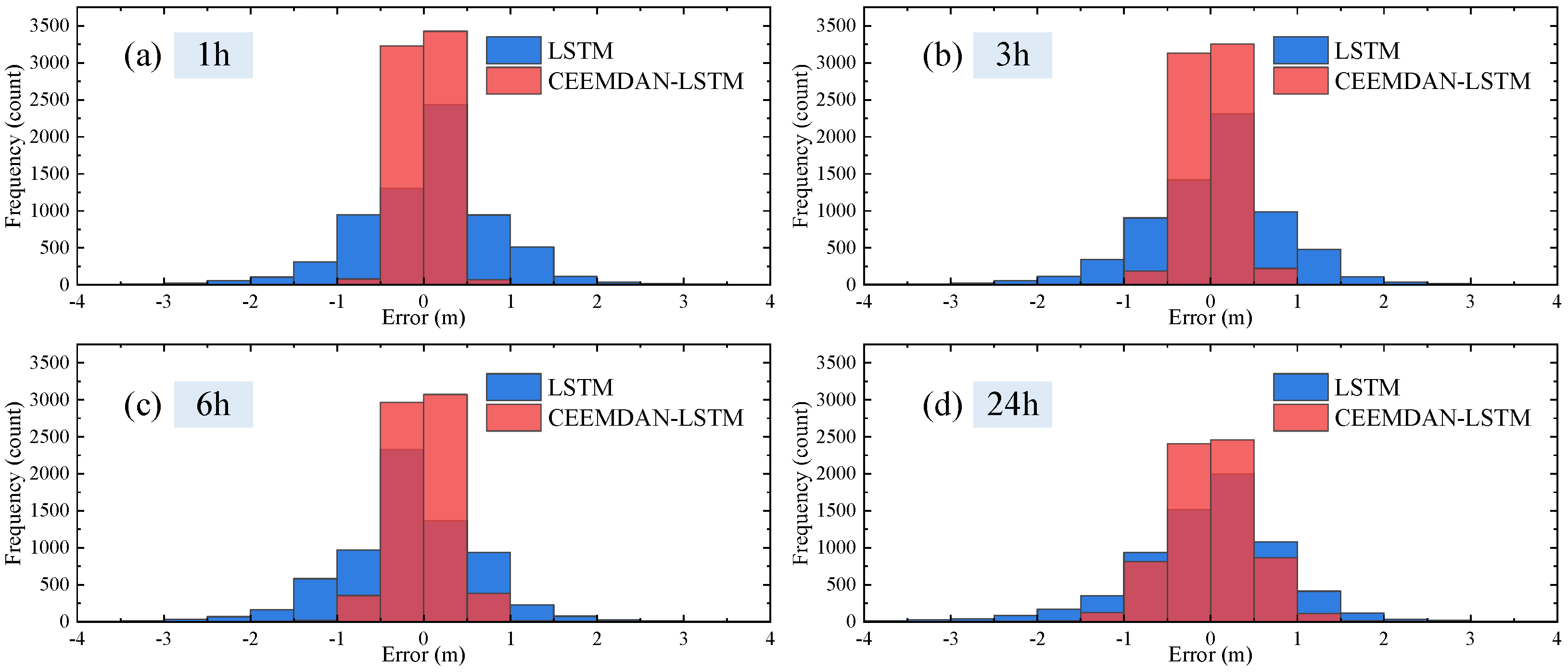
• When the CEEMDAN-LSTM model is used for SWH forecasting, the forecasts show the general trend of the waves and better capture fluctuations in local peaks and troughs, and the forecast accuracy is greatly improved.
• Through the CEEMDAN algorithm, the original SWH data is decomposed into high frequency sinusoidal intermittent signals, intermediate frequency sinusoidal intermittent signals and low frequency broad period signals.
• The integrated CEEMDAN-LSTM joint model outperforms the LSTM in terms of accuracy, as CEEMDAN is able to decompose the original nonlinear and nonstationary SWH into various IMFs, thus enabling the LSTM to better capture changes in trends.
• When the forecast duration is 1 h, CEEMDAN-LSTM has the most significant improvement over LSTM, with 71.91% of RMSE, 68.46% of MAE and 6.80% of NSE, respectively.
• Even with a 24-h advance, CEEMDAN-LSTM still improves 53.44%, 40.31% and 7.91% over LSTM in terms of RMSE, MAE and NSE. CEEMDAN-LSTM is still substantially better than LSTM.
• Accurate SWH predictions are crucial for the development and commercial viability of wave energy conversion as a clean energy source. The results of the CEEMDAN-LSTM predictions have also been discussed for this paper, and the results were satisfactory.

However, the LSTM still fails to make effective predictions for rapid changes in high frequency (HF) IMFs. This is because the HF component still contains the original undecomposed SWH signal, which can interfere with the accuracy of the model. This may be due to the fact that the predictions do not take into account factors such as ocean currents, sea breeze wind speed and wind direction. Further improvements can therefore be made to the model in this respect. Despite the abovementioned advantages of our model, we do not take into account information on the geographical location of the ShiDao in this paper. This means that the integrated CEEMDAN-LSTM joint model only models the temporal information, not the spatial information. Furthermore, the waves in all regions of the earth are not independent of each other; there is some coupling between them. Further research from the perspective of extracting spatial information can be continued in the future.

In summary, the integrated CEEMDAN-LSTM joint model can provide more accurate SWH predictions, which can improve real-time scheduling for fishing vessel operations, wave energy generation or other marine engineering maintenance and operations.

References

1. Taylor, J.W.; Jeon, J. Probabilistic forecasting of wave height for offshore wind turbine maintenance. Eur. J. Oper. Res. 2018, 267, 877–890. [Google Scholar] [CrossRef]
2. Guillou, N.; Lavidas, G.; Chapalain, G. Wave Energy Resource Assessment for Exploitation—A Review. J. Mar. Sci. Eng. 2020, 8, 705. [Google Scholar] [CrossRef]
3. Wimalaratna, Y.P.; Hassan, A.; Afrouzi, H.N.; Mehranzamir, K.; Ahmed, J.; Siddique, B.M.; Liew, S.C. Comprehensive review on the feasibility of developing wave energy as a renewable energy resource in Australia. Clean. Energy Syst. 2022, 3, 100021. [Google Scholar] [CrossRef]
4. Guillou, N.; Chapalain, G. Annual and seasonal variabilities in the performances of wave energy converters. Energy 2018, 165, 812–823. [Google Scholar] [CrossRef] [Green Version]
5. Chen, C.; Sasa, K.; Prpić-Oršić, J.; Mizojiri, T. Statistical analysis of waves’ effects on ship navigation using high-resolution numerical wave simulation and shipboard measurements. Ocean. Eng. 2021, 229, 108757. [Google Scholar] [CrossRef]
6. Saetre, C.; Tholo, H.; Hovdenes, J.; Kocbach, J.; Hageberg, A.A.; Klepsvik, I.; Aarnes, O.J.; Furevik, B.R.; Magnusson, A.K. Directional wave measurements from navigational buoys. Ocean. Eng. 2023, 268, 113161. [Google Scholar] [CrossRef]
7. Figueiredo, R.; Fazeres-Ferradosa, T.; Chambel, J.; Rosa Santos, P.; Taveira Pinto, F. How does the selection of wave hindcast datasets and statistical models influence the probabilistic design of offshore scour protections? Ocean. Eng. 2022, 266, 113123. [Google Scholar] [CrossRef]
8. Wu, M.; De Vos, L.; Arboleda Chavez, C.E.; Stratigaki, V.; Whitehouse, R.; Baelus, L.; Troch, P. A study of scale effects in experiments of monopile scour protection stability. Coast. Eng. 2022, 178, 104217. [Google Scholar] [CrossRef]
9. Zhang, Y.; Chen, Y.; Qi, Z.; Wang, S.; Zhang, J.; Wang, F. A hybrid forecasting system with complexity identification and improved optimization for short-term wind speed prediction. Energy Convers. Manag. 2022, 270, 116221. [Google Scholar] [CrossRef]
10. Zheng, C.-w.; Li, X.-h.; Azorin-Molina, C.; Li, C.-y.; Wang, Q.; Xiao, Z.-n.; Yang, S.-b.; Chen, X.; Zhan, C. Global trends in oceanic wind speed, wind-sea, swell, and mixed wave heights. Appl. Energy 2022, 321, 119327. [Google Scholar] [CrossRef]
11. Fazeres-Ferradosa, T.; Taveira-Pinto, F.; Vanem, E.; Reis, M.T.; Neves, L.D. Asymmetric copula–based distribution models for met-ocean data in offshore wind engineering applications. Wind. Eng. 2018, 42, 304–334. [Google Scholar] [CrossRef] [Green Version]
12. Fazeres-Ferradosa, T.; Welzel, M.; Schendel, A.; Baelus, L.; Santos, P.R.; Pinto, F.T. Extended characterization of damage in rubble mound scour protections. Coast. Eng. 2020, 158, 103671. [Google Scholar] [CrossRef]
13. Duan, W.Y.; Han, Y.; Huang, L.M.; Zhao, B.B.; Wang, M.H. A hybrid EMD-SVR model for the short-term prediction of significant wave height. Ocean. Eng. 2016, 124, 54–73. [Google Scholar] [CrossRef]
14. Ye, Y.; Wang, L.; Wang, Y.; Qin, L. An EMD-LSTM-SVR model for the short-term roll and sway predictions of semi-submersible. Ocean. Eng. 2022, 256, 111460. [Google Scholar] [CrossRef]
15. Nie, Z.; Shen, F.; Xu, D.; Li, Q. An EMD-SVR model for short-term prediction of ship motion using mirror symmetry and SVR algorithms to eliminate EMD boundary effect. Ocean. Eng. 2020, 217, 107927. [Google Scholar] [CrossRef]
16. Janssen, P.A.E.M. Progress in ocean wave forecasting. J. Comput. Phys. 2008, 227, 3572–3594. [Google Scholar] [CrossRef]
17. Myrhaug, D.; Fouques, S. A joint distribution of significant wave height and characteristic surf parameter. Coast. Eng. 2010, 57, 948–952. [Google Scholar] [CrossRef]
18. Sezer, A.; Asma, S. Statistical power of an information-based test and its application to wave height data. Comput. Geosci. 2010, 36, 1316–1324. [Google Scholar] [CrossRef]
19. Nam, B.W.; Kim, J.-S.; Hong, S.Y. Numerical investigation on hopf bifurcation problem for nonlinear dynamics of a towed vessel in calm water and waves. Ocean. Eng. 2022, 266, 112661. [Google Scholar] [CrossRef]
20. Zhao, L.; Li, Z.; Qu, L. Forecasting of Beijing PM2.5 with a hybrid ARIMA model based on integrated AIC and improved GS fixed-order methods and seasonal decomposition. Heliyon 2022, 8, e12239. [Google Scholar] [CrossRef]
21. Yang, S.; Deng, Z.; Li, X.; Zheng, C.; Xi, L.; Zhuang, J.; Zhang, Z.; Zhang, Z. A novel hybrid model based on STL decomposition and one-dimensional convolutional neural networks with positional encoding for significant wave height forecast. Renew. Energy 2021, 173, 531–543. [Google Scholar] [CrossRef]
22. Özger, M. Significant wave height forecasting using wavelet fuzzy logic approach. Ocean. Eng. 2010, 37, 1443–1451. [Google Scholar] [CrossRef]
23. Shahabi, S.; Khanjani, M.J. Modelling of significant wave height using wavelet transform and GMDH. In Proceedings of the 36th IAHR World Congress, Hague, The Netherlands, 28 June 2015. [Google Scholar]
24. Ali, M.; Prasad, R. Significant wave height forecasting via an extreme learning machine model integrated with improved complete ensemble empirical mode decomposition. Renew. Sustain. Energy Rev. 2019, 104, 281–295. [Google Scholar] [CrossRef]
25. Kim, S.; Takeda, M.; Mase, H. GMDH-based wave prediction model for one-week nearshore waves using one-week forecasted global wave data. Appl. Ocean. Res. 2021, 117, 102859. [Google Scholar] [CrossRef]
26. Camus, P.; Herrera, S.; Gutiérrez, J.M.; Losada, I.J. Statistical downscaling of seasonal wave forecasts. Ocean. Model. 2019, 138, 1–12. [Google Scholar] [CrossRef]
27. Raj, N.; Brown, J. An EEMD-BiLSTM Algorithm Integrated with Boruta Random Forest Optimiser for Significant Wave Height Forecasting along Coastal Areas of Queensland, Australia. Remote Sens. 2021, 13, 1456. [Google Scholar] [CrossRef]
28. Zilong, T.; Yubing, S.; Xiaowei, D. Spatial-temporal wave height forecast using deep learning and public reanalysis dataset. Appl. Energy 2022, 326, 120027. [Google Scholar] [CrossRef]
29. Deka, P.C.; Prahlada, R. Discrete wavelet neural network approach in significant wave height forecasting for multistep lead time. Ocean. Eng. 2012, 43, 32–42. [Google Scholar] [CrossRef]
30. Ma, J.; Xue, H.; Zeng, Y.; Zhang, Z.; Wang, Q. Significant wave height forecasting using WRF-CLSF model in Taiwan strait. Eng. Appl. Comput. Fluid Mech. 2021, 15, 1400–1419. [Google Scholar] [CrossRef]
31. Gao, R.; Li, R.; Hu, M.; Suganthan, P.N.; Yuen, K.F. Dynamic ensemble deep echo state network for significant wave height forecasting. Appl. Energy 2023, 329, 120261. [Google Scholar] [CrossRef]
32. Yao, J.; Wu, W. Wave height forecast method with multi-step training set extension LSTM neural network. Ocean. Eng. 2022, 263, 112432. [Google Scholar] [CrossRef]
33. Li, X.; Cao, J.; Guo, J.; Liu, C.; Wang, W.; Jia, Z.; Su, T. Multi-step forecasting of ocean wave height using gate recurrent unit networks with multivariate time series. Ocean. Eng. 2022, 248, 110689. [Google Scholar] [CrossRef]
34. Sun, Z.; Zhao, M.; Zhao, G. Hybrid model based on VMD decomposition, clustering analysis, long short memory network, ensemble learning and error complementation for short-term wind speed forecasting assisted by Flink platform. Energy 2022, 261, 125248. [Google Scholar] [CrossRef]
35. Luo, Q.-R.; Xu, H.; Bai, L.-H. Prediction of significant wave height in hurricane area of the Atlantic Ocean using the Bi-LSTM with attention model. Ocean. Eng. 2022, 266, 112747. [Google Scholar] [CrossRef]
36. Liu, Y.; Zhang, X.; Chen, G.; Dong, Q.; Guo, X.; Tian, X.; Lu, W.; Peng, T. Deterministic wave prediction model for irregular long-crested waves with Recurrent Neural Network. J. Ocean. Eng. Sci. 2022. [Google Scholar] [CrossRef]
37. Ji, C.; Zhang, C.; Hua, L.; Ma, H.; Nazir, M.S.; Peng, T. A multi-scale evolutionary deep learning model based on CEEMDAN, improved whale optimization algorithm, regularized extreme learning machine and LSTM for AQI prediction. Environ. Res. 2022, 215, 114228. [Google Scholar] [CrossRef]
38. Zhang, C.; Hua, L.; Ji, C.; Shahzad Nazir, M.; Peng, T. An evolutionary robust solar radiation prediction model based on WT-CEEMDAN and IASO-optimized outlier robust extreme learning machine. Appl. Energy 2022, 322, 119518. [Google Scholar] [CrossRef]
39. Hu, C.; Zhao, Y.; Jiang, H.; Jiang, M.; You, F.; Liu, Q. Prediction of ultra-short-term wind power based on CEEMDAN-LSTM-TCN. Energy Rep. 2022, 8, 483–492. [Google Scholar] [CrossRef]
40. Wang, N.; Nie, J.; Li, J.; Wang, K.; Ling, S. A compression strategy to accelerate LSTM meta-learning on FPGA. ICT Express 2022, 8, 322–327. [Google Scholar] [CrossRef]
41. Mushtaq, E.; Zameer, A.; Umer, M.; Abbasi, A.A. A two-stage intrusion detection system with auto-encoder and LSTMs. Appl. Soft Comput. 2022, 121, 108768. [Google Scholar] [CrossRef]
42. Huang, N.; Shen, Z.; Long, S.; Wu ML, C.; Shih, H.; Zheng, Q.; Yen, N.-C.; Tung, C.-C.; Liu, H. The empirical mode decomposition and the Hilbert spectrum for nonlinear and non-stationary time series analysis. Proc. R. Soc. London. Ser. A Math. Phys. Eng. Sci. 1998, 454, 903–995. [Google Scholar] [CrossRef]
43. Wu, Z.; Huang, N.E. Ensemble Empirical Mode Decomposition: A Noise-Assisted Data Analysis Method. Adv. Data Sci. Adapt. Anal. 2009, 1, 1–41. [Google Scholar] [CrossRef]
44. Xu, K.; Niu, H. Do EEMD based decomposition-ensemble models indeed improve prediction for crude oil futures prices? Technol. Forecast. Soc. Change 2022, 184, 121967. [Google Scholar] [CrossRef]
45. Ran, P.; Dong, K.; Liu, X.; Wang, J. Short-term load forecasting based on CEEMDAN and Transformer. Electr. Power Syst. Res. 2023, 214, 108885. [Google Scholar] [CrossRef]
46. Li, K.; Huang, W.; Hu, G.; Li, J. Ultra-short term power load forecasting based on CEEMDAN-SE and LSTM neural network. Energy Build. 2023, 279, 112666. [Google Scholar] [CrossRef]
47. Vardaroglu, M.; Gao, Z.; Avossa, A.M.; Ricciardelli, F. Validation of a TLP wind turbine numerical model against model-scale tests under regular and irregular waves. Ocean. Eng. 2022, 256, 111491. [Google Scholar] [CrossRef]
48. Koivu, A.; Kakko, J.-P.; Mäntyniemi, S.; Sairanen, M. Quality of randomness and node dropout regularization for fitting neural networks. Expert Syst. Appl. 2022, 207, 117938. [Google Scholar] [CrossRef]
49. Röhmel, J. The permutation distribution of the Friedman test. Comput. Stat. Data Anal. 1997, 26, 83–99. [Google Scholar] [CrossRef]
50. Ma, J.; Xia, D.; Wang, Y.; Niu, X.; Jiang, S.; Liu, Z.; Guo, H. A comprehensive comparison among metaheuristics (MHs) for geohazard modeling using machine learning: Insights from a case study of landslide displacement prediction. Eng. Appl. Artif. Intell. 2022, 114, 105150. [Google Scholar] [CrossRef]
51. Berčič, G. The universality of Friedman’s isoconversional analysis results in a model-less prediction of thermodegradation profiles. Thermochim. Acta 2017, 650, 1–7. [Google Scholar] [CrossRef]
52. Bozorgzadeh, L.; Bakhtiari, M.; Shani Karam Zadeh, N.; Esmaeeldoust, M. Forecasting of Wind-Wave Height by Using Adaptive Neuro-Fuzzy Inference System and Decision Tree. J. Soft Comput. Civ. Eng. 2019, 3, 22–36. [Google Scholar]
53. Chen, S.-T.; Wang, Y.-W. Improving Coastal Ocean Wave Height Forecasting during Typhoons by using Local Meteorological and Neighboring Wave Data in Support Vector Regression Models. J. Mar. Sci. Eng. 2020, 8, 149. [Google Scholar] [CrossRef] [Green Version]
54. Zhou, S.; Bethel, B.J.; Sun, W.; Zhao, Y.; Xie, W.; Dong, C. Improving Significant Wave Height Forecasts Using a Joint Empirical Mode Decomposition–Long Short-Term Memory Network. J. Mar. Sci. Eng. 2021, 9, 744. [Google Scholar] [CrossRef]
55. Nasiri, H.; Ebadzadeh, M.M. MFRFNN: Multi-Functional Recurrent Fuzzy Neural Network for Chaotic Time Series Prediction. Neurocomputing 2022, 507, 292–310. [Google Scholar] [CrossRef]
56. Nasiri, H.; Ebadzadeh, M.M. Multi-step-ahead Stock Price Prediction Using Recurrent Fuzzy Neural Network and Variational Mode Decomposition. arXiv 2022, arXiv:2212.14687. [Google Scholar]
Figure 1. The network structure diagram of LSTM.
Jmse 11 00435 g001
Figure 2. Flowchart of the integrated CEEMDAN-LSTM joint prediction model.
Jmse 11 00435 g002
Figure 3. Distribution of ShiDao monitoring station on the east coast of China.
Jmse 11 00435 g003
Figure 4. Significant wave height time series of ShiDao effective data.
Jmse 11 00435 g004
Figure 5. Violin plot and frequency distribution histogram of effective data.
Jmse 11 00435 g005
Figure 6. Comparison of the components of the violin and box plots.
Jmse 11 00435 g006
Figure 7. Box plot of SWH effective data for calendar year.
Jmse 11 00435 g007
Figure 8. Comparison of ShiDao effective data in the time domain for the IMFs component of SWH sequence by EMD algorithm.
Jmse 11 00435 g008
Figure 9. Comparison of ShiDao effective data in the time domain for the IMFs component of SWH sequence by CEEMDAN algorithm.
Jmse 11 00435 g009
Figure 10. Comparison of ShiDao effective data in the frequency domain for the IMFs component of SWH sequence by EMD algorithm.
Jmse 11 00435 g010
Figure 11. Comparison of ShiDao effective data in the frequency domain for the IMFs component of SWH sequence by CEEMDAN algorithm.
Jmse 11 00435 g011
Figure 12. Comparison of LSTM (blue) and CEEMDAN-LSTM (red) SWH (m) forecasts with (a) 1-, (b) 3-, (c) 6- and (d) 24-h window measured values (black). Subplots provide a closer examination of the offset between measured and predicted values in (e) 1-, (f) 3-, (g) 6- and (h) 24-h windows.
Jmse 11 00435 g012
Figure 13. Comparison of ShiDao measured and predicted values by LSTM (blue) and CEEMDAN-LSTM (red) SWH (m) forecasts with (a) 1-, (b) 3-, (c) 6- and (d) 24-h window.
Jmse 11 00435 g013
Figure 14. Comparison of measured (black) and CEEMDAN-LSTM predicted (red) values with SWH forecasts of (a) IMF1, (b) IMF5, (c) IMF9, (d) IMF13 and (e) IMF17 in 1-h window.
Jmse 11 00435 g014
Figure 15. Wave energy estimate results of upper-estimate (green) and lower-estimate (yellow) with 5-m SWH measured values (black) in 2–6-s wave period.
Jmse 11 00435 g015
Figure 16. Wave energy estimate results of upper-estimate (green) and lower-estimate (yellow) of CEEMDAN-LSTM prediction (red) in comparison with measured values (black) in 5-s wave period.
Jmse 11 00435 g016