A Lightweight Network Model Based on an Attention Mechanism for Ship-Radiated Noise Classification

Abstract

Recently, deep learning has been widely used in ship-radiated noise classification. To improve classification efficiency, avoiding high computational costs is an important research direction in ship-radiated noise classification. We propose a lightweight squeeze and excitation residual network 10 (LW-SEResNet10). In ablation experiments of LW-SEResNet10, the use of ResNet10 instead of ResNet18 reduced 56.1% of parameters, while the accuracy is equivalent to ResNet18. The improved accuracy indicates that the ReLU6 enhanced the model stability, and an attention mechanism captured the channel dependence. The ReLU6 activation function does not introduce additional parameters, and the number of parameters introduced by the attention mechanism accounts for 0.2‰ of the model parameters. The 3D dynamic MFCC feature performs better than MFCC, Mel-spectrogram, 3D dynamic Mel-spectrogram, and CQT. Moreover, the LW-SEResNet10 model is also compared with ResNet and two classic lightweight models. The experimental results show that the proposed model achieves higher classification accuracy and is lightweight in terms of not only the model parameters, but also the time consumption. LW-SEResNet10 also outperforms the state-of-the-art model CRNN-9 by 3.1% and ResNet by 3.4% and has the same accuracy as AudioSet pretrained STM, which achieves the trade-off between accuracy and model efficiency.

1. Introduction

Ship-radiated noise includes airborne noise and underwater noise. Airborne noise mainly influences human health [1,2]. For military and security reasons, we pay more attention to underwater noise. At present, deep learning methods applied to Ship-radiated noise featuring learning and classification has become a hot research topic [3,4,5,6,7,8]. Ship-radiated noise featuring learning and classification is an important research direction of underwater acoustic target recognition. From the perspective of sound generation mechanisms, the target radiated noise is considered to be mainly composed of mechanical noise, propeller noise, and hydrodynamic noise [9]. The difference in the target radiated noise of different types can be reflected in the following aspects: (1) mechanical noise generated by different shipborne mechanical equipment; (2) propeller radiation characteristics being different due to different propeller parameters; and (3) the difference in hydrodynamic noise caused by different hull structures. Therefore, the ship-radiated noise can reflect ship attributes and be used to classify ship categories. Compared with shallow models, deep neural networks can learn more abstract and invariant features from a large dataset [10,11]. Therefore, deep learning can not only automatically learn feature representations from the raw signal, but can also perform further deep feature extraction and even feature fusion based on some artificial feature parameters such as Mel Frequency Cepstrum Coefficient (MFCC) [12], constant Q transform (CQT) [13], wavelet feature [14,15], DEMON spectrum and LOFAR spectrum [16], and high-order spectral features [17,18]. Those traditional feature analysis methods effectively reduce information redundancy and the computational cost of the back-end model.

Due to the difficulty and high cost of marine experiments, the effective samples of ship-radiated noise data are insufficient [19]. The insufficient data would lead to over-fitting of the large-scale deep network model, which is difficult to converge, ultimately affecting the classification accuracy [20]. To solve this problem, Gao et al. [21] used a deep convolutional generative adversarial network (DCGAN) to expand the training set, improving the classification effect. Jiang et al. [22] proposed the modified DCGAN model to augment data for targets with a small sample size. Using GAN to generate ship-radiated noise data can effectively solve the problem of scarcity of samples, but the training of generative networks is time-consuming. Yang et al. [12] proposed an improved competitive deep belief network (DBN), which addresses the problem of insufficient training samples by pre-training the DBN with a large amount of unlabeled ship-radiated noise. Jin et al. [23] used a CNN pre-trained on the ImageNet dataset [24] and fine-tuned the network with fish image data with a small sample size to effectively solve the underwater image classification problem. These pre-training methods as transfer learning methods require considering the similarity between data, tasks, or models and need preload model parameters. A measurement of similarity needs to be defined. The negative transfer may occur when the source domain data and target domain data are not similar or when the deep model is not good enough to find a transferable feature. For our study, a lightweight network is designed to improve classification accuracy in a small sample condition.

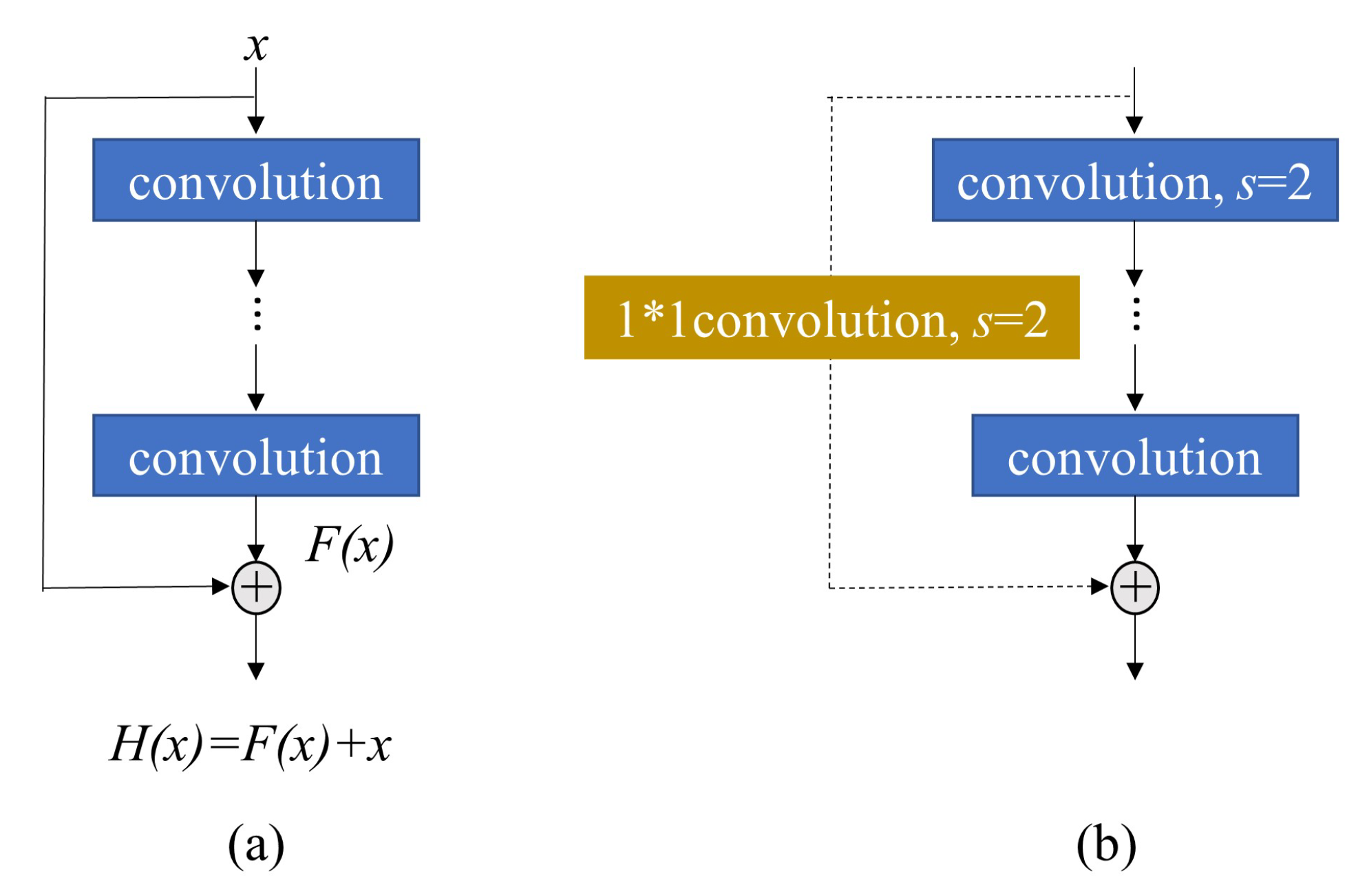
The large-scale residual network (ResNet) [25] is redundant in the field of computer vision. Gao et al. [26] randomly removed many layers of ResNet during the training process, which did not affect the convergence of the algorithm, and the removal of the middle layers had little effect on the final results, illustrating that ResNet has redundancy. For underwater acoustic target recognition, a depth search experiment for a multiscale residual deep neural network (MSRDN) [27] was conducted. The results prove that the original MSRDN with 101 depths is redundant. Xue et al. [28] observed that the recognition rate will decrease by increasing the number of residual layers, which indicates the redundancy of ResNet. Therefore, it is feasible to reduce the model parameters while maintaining the model performance. For our work, a reduction of the model parameter is realized by shrinking the number of residual units in ResNet.

Meanwhile, large-scale deep models have the problem of high computation costs [29]. For practical applications, the trade-off between accuracy and model efficiency is necessary. The efficiency is defined with lower computation cost or time cost. To develop efficient deep models, recent works in the field of computer vision usually focus on structural design [30,31], low-rank factorization [32], and knowledge distillation [33,34]. For underwater acoustic target recognition, Lei et al. [35] proposed that avoiding high computational costs is an important future direction of underwater acoustic information processing. Jiang et al. 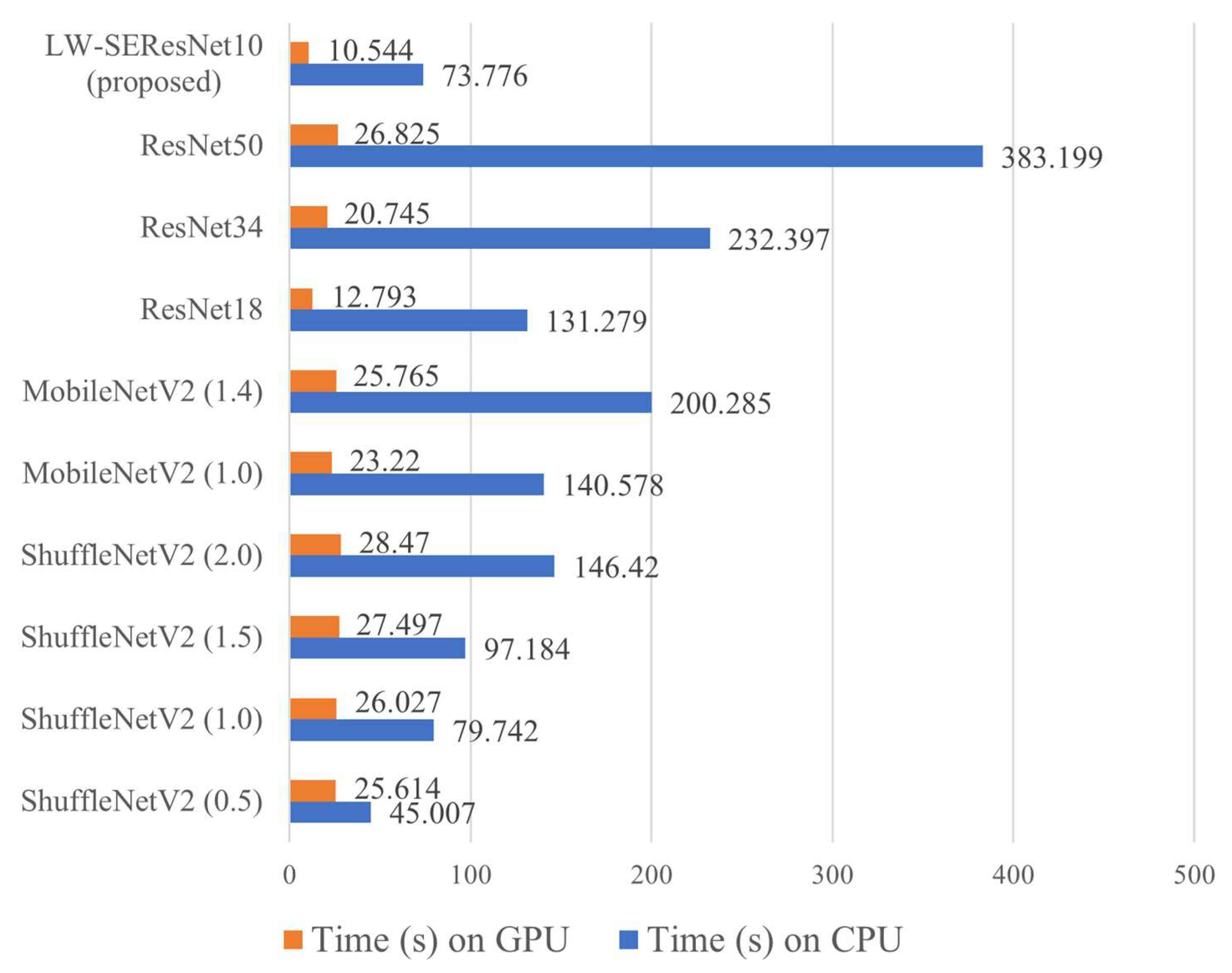[22] proposed the S-ResNet model to obtain good classification accuracy while significantly reducing the complexity of the model and achieving a good trade-off between classification accuracy and model complexity. Meanwhile, the parameters and floating-point operations (FLOPs) of the model are used to measure the model’s complexity. However, on the actual equipment, due to a variety of optimization calculation operations, the theoretical parameters and FLOPs cannot accurately measure the actual time consumption of the model [31]. Therefore, for our study, in addition to using the theoretical parameters, we will also measure the complexity of the model according to the actual time consumption. Tian et al. [36] designed a lightweight MSRDN using lightweight network design techniques, in which 64.18% of parameters and 79.45% of FLOPs are reduced from the original MSRDN with a small loss of accuracy. Meanwhile, the time cost under the same hardware and software platforms was conducted. For our study, we will measure time costs on different platforms.

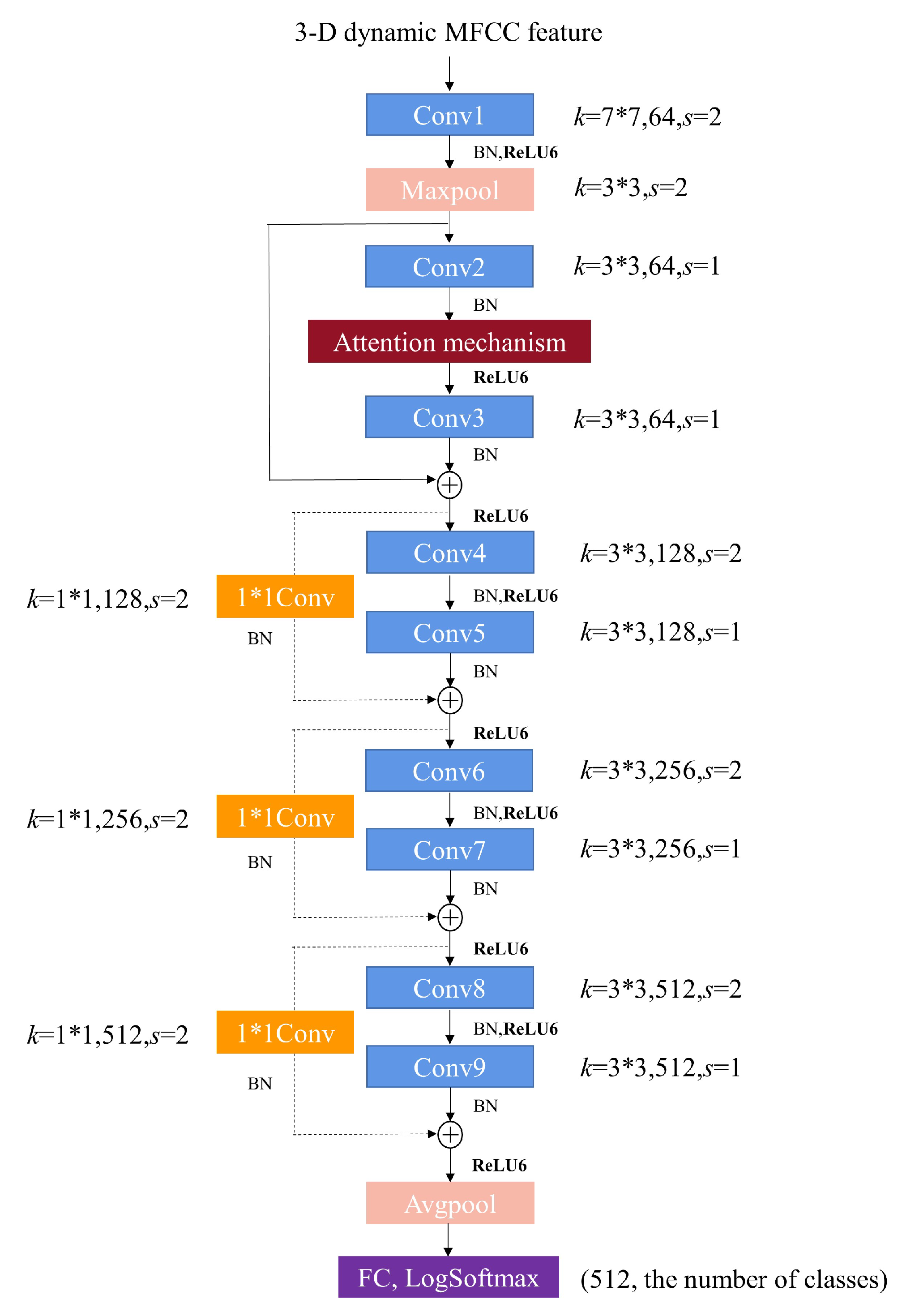
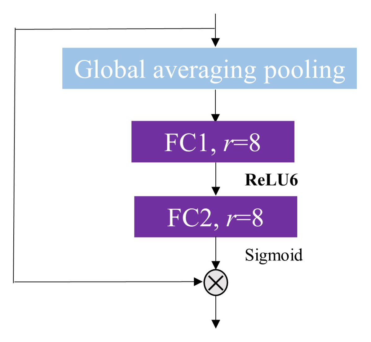
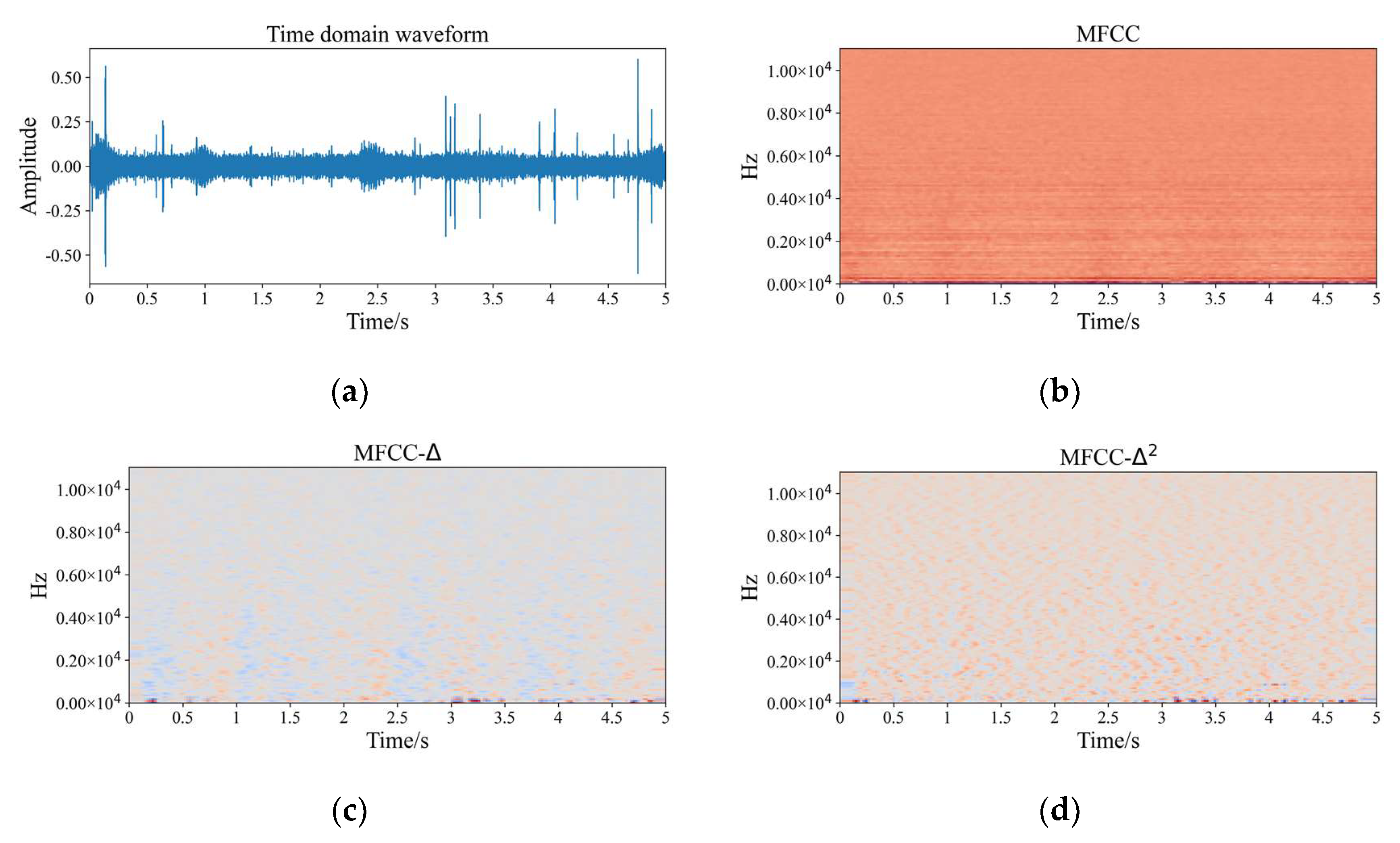
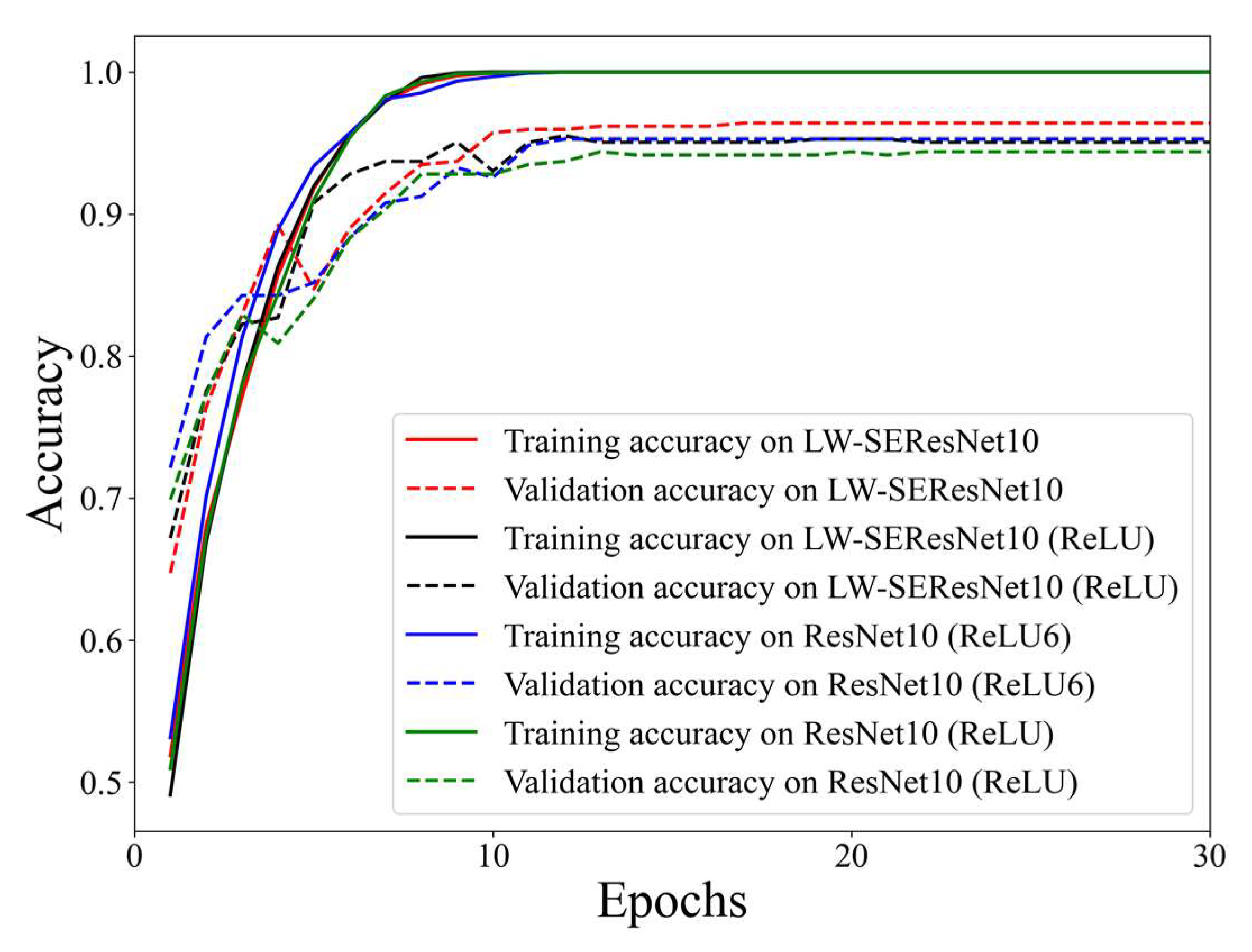
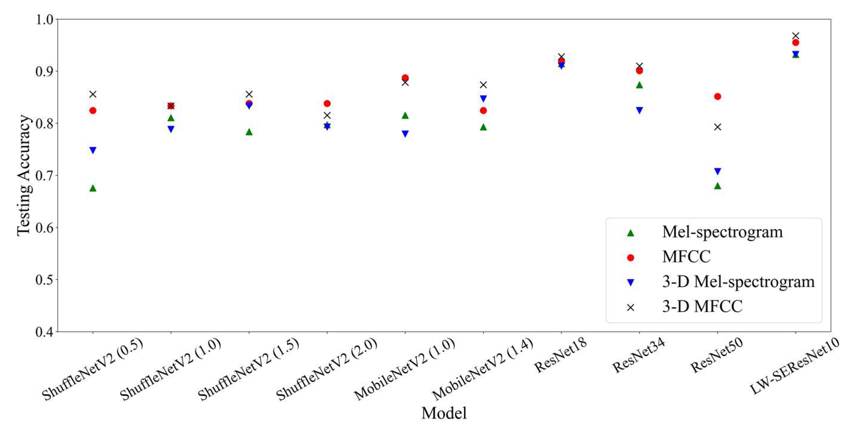
Our study utilizes the structural design technique to design our lightweight network. Lightweight networks are defined as having fewer model parameters or faster run times. The proposed model, namely lightweight squeeze and excitation residual network 10 (LW-SEResNet10), aims to inhibit overfitting and achieve high accuracy and high efficiency. Firstly, shrinking the number of residual units in the ResNet reduces the number of parameters. Secondly, the attention mechanism called “squeeze-excitation” (SE) block [37] with low parameters is introduced into the proposed model. The attention mechanism [38] can help the network give different weights to each part of the input features, extracting more critical and important information. The attention mechanism is integrated into a residual unit structure, which helps to capture the correlation between features, and the representation generated by convolution networks can be strengthened. 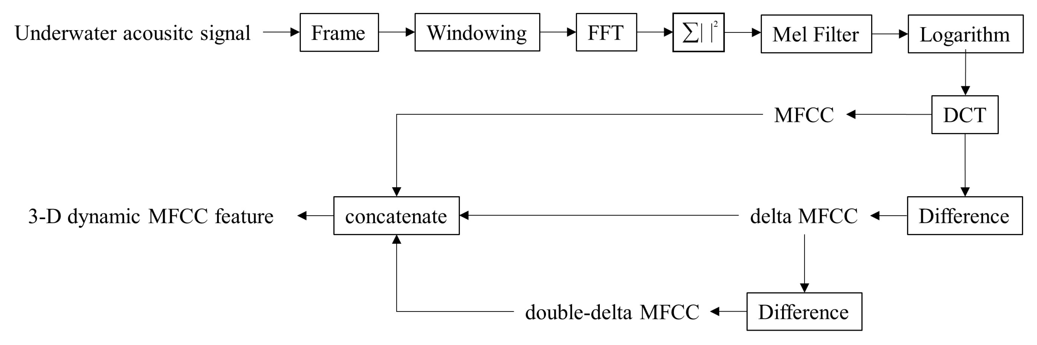Thirdly, the ReLU6 activation function [39] is employed to increase the model stability. The ReLU6 activation function does not introduce additional parameters. Moreover, the 3D dynamic MFCC feature is used as the input of the proposed model. The 3D dynamic MFCC feature effectively compresses the raw time-domain information of the target radiated noise signal, while extracting the higher-order dynamic time information of the signal. To verify the lightweight nature and superiority of our proposed model, we compare the proposed model with the ResNet and the classical lightweight network models MobileNet V2 [30] and ShuffleNet V2 [31] in the field of computer vision in terms of parameters, time consumption, accuracy, and noise mismatch.

The remainder of this article is organized as follows. Section 2 provides an overview of our ship-radiated noise classification method in detail. Experiments are presented in Section 3, and Section 4 concludes this article.

2. System Overview

This section mainly describes the proposed ship-radiated noise classification framework. The first part introduces the proposed lightweight model. The second part introduces the extraction method of the 3D dynamic MFCC feature.

2.1. The Design of the Proposed Model

2.1.1. Residual Network (ResNet)

ResNet [25] is proposed to deal with deep neural network degradation. In contrast with ordinary neural networks, the ResNet model implements a cross-layer connection by residual unit structure. The architecture of the residual unit is shown in Figure 1. The basic residual unit is shown in Figure 1a. It can be seen that the residual unit contains two types of connections; one is a non-linear mapping connection similar to an ordinary neural network, which generally consists of two to three convolutional layers, and the other is a short-cut connection. The input of a residual unit is denoted as x, the nonlinear mapping as F(x) (i.e., the residual mapping), and H(x) as the computed result of the residual unit, then their arithmetic relationship can be expressed as:

$$\begin{array}{ll}H(x)& =x+F(x)\\ & =x+w_N\delta (w_{N-1}(\delta (\dots \delta (w_{1}x))))\end{array}$$

(1)

where $w_1,w_2,\dots ,w_N$ are the weights of convolutional layers and $\delta$ is the ReLU activation function. When the residual unit performs the backpropagation, the gradient is expressed as:

$$\frac{\partial H(x)}{\partial x}=1+\frac{\partial (w_N\delta (w_{N-1}(\delta (\dots \delta (w_{1}x)))))}{\partial x}$$

(2)

Due to the existence of constant 1, the phenomenon of gradient disappearance during backpropagation is avoided. ResNet learns F(x) + x by iteration training, rather than learning H(x) directly. Learning the residual F(x) is easier to converge than learning the mapping between x, and H(x) directly, and can achieve higher classification accuracy. Figure 1b shows the downsampled residual unit, with dashed lines indicating short-cut connections. In ResNet, not all residual units have pooling layers, so a convolutional layer is needed to implement downsampling. This is implemented by setting the stride of the convolutional layer to 2 (s = 2) to change the shape of the residual mapping. Meanwhile, since the residual units are to be summed, the shape and dimension of the input x and the residual mapping F(x) must be consistent. When the residual mapping F(x) is downsampled, downsampling of x is required in the short-cut connection, which is implemented by setting a 1 × 1 convolution layer with a stride of 2 (s = 2) and then adding the downsampled x and F(x).

2.1.2. The Proposed Lightweight Squeeze and Excitation Residual Network 10 (LW-SEResNet10)

In this study, ResNet18 is shrunk in order to reduce the number of parameters. The proposed model is shown in Figure 2. The 18-layer ResNet is reduced to 10 layers (including nine convolutional layers and one fully connected layer). The input is the extracted 3D dynamic MFCC feature, and the classification layer is a fully connected layer (FC) with LogSoftmax, which outputs the probability distribution of each sample corresponding to all classes as the basis for judging the sample classes. The LogSoftmax function can be expressed as follows:

$$\begin{array}{ll}\mathrm{LogSoftmax}(x_i)& =\log (\frac{\exp (x_i)}{{\displaystyle \sum _{j=1}^N\exp (x_j)}})i=1,2,\dots ,N\\ & =\log (\exp (x_i))-\log ({\displaystyle \sum _{j=1}^N\exp (x_j)})\\ & =x_i-\log ({\displaystyle \sum _{j=1}^N\exp (x_j)})\end{array}$$

(3)

where x denotes the output of the fully connected layer and the dimension is N. N corresponds to the number of classes. LogSoftmax(x_i) is the probability that the predicted sample x belongs to class i. The logarithm behind Softmax changes the multiplication to addition to reduce the amount of calculation while ensuring the monotonicity of the function.

In Figure 2, the nine convolutional layers are named Conv1 to Conv9, k denotes the size of the convolutional kernel, s denotes the stride, and 64, 128, 256, and 512 are the number of convolutional kernels. Max pooling (Maxpool) and averaging pooling (Avgpool) are implemented for downsampling. Batch normalization (BN) operation is applied behind the convolutional layer. By normalizing the data of each batch, the network convergence speed is accelerated while preventing the gradient from disappearing and exploding in the network. Since ReLU uses x for linear activation in the region of x > 0, which may cause values that are too large after activation and affect the stability of the proposed model. To offset the linear growth part of the ReLU activation function, this paper uses the ReLU6 [39] activation function instead of the ReLU activation function. ReLU6 limits linear activation to a range of 0 to 6, preventing the values from exploding. The ReLU6 activation function can be expressed as follows:

$$\mathrm{ReLU}6(x)=\min (max(0,x),6)$$

(4)

In addition, the proposed model integrates the SE block [37] operation as an attention mechanism after the Conv2 layer to capture the channel dependencies, the specific framework shown in Figure 3. Firstly, a global averaging pooling operation [40] aggregates feature maps (the output of the Conv2 layer) to generate channel statistics, which is named the “squeeze” operation. The “squeeze” formula is expressed as follows:

$$z_c=\frac{1}{H\times W}{\displaystyle \sum _{i=1}^H{\displaystyle \sum _{j=1}^W{u}_c(i,j)}}$$

(5)

where $z_c\in R^c$ denotes the channel statistics and C is the number of channels. H and W are the height and width of the feature maps. The feature maps are expressed as $U=[u_1,u_2,\dots ,u_c]$. The result of this step is to collect the global information of all feature maps on ship-radiated noise signals.

Secondly, the “excitation” operation fully captures the channel dependence on all feature maps on ship-radiated noise signals. Two fully connected operations (FC1 layer and FC2 layer) with nonlinear activation function ReLU6 encode and decode the channel statistics, respectively. The operations, as an unsupervised autoencoder, reconstruct channel statistics adaptively, which represents the channel information effectively. A sigmoid activation function is inserted to normalize the reconstructed channel statistics. The “excitation” formula is expressed as follows:

$$s=\sigma (W_2\delta (W_{1}z))$$

(6)

where s denotes the channel statistics after the “excitation” operation, $\delta$ denotes the ReLU6 function, $\sigma$ denotes a sigmoid activation function, $W_1\in R^{\frac{C}{r}\times C}$ and $W_2\in R^{C\times \frac{C}{r}}$. r denotes the reduction ratio, which is set to 8.

The “excitation” operation can be regarded as a soft threshold, which is similar to the gate mechanism of long short-term memory, applied to complete the network "forget" and “memory” functions. Finally, the dot product operation is performed on the channel statistics and $U$ (the feature maps after the Conv2 layer) to recalibrate the channel weights $U$. The soft threshold mechanism enables highlighting the weight of important information in channel statistics. These two operations can be regarded as an attention mechanism for channel information.

The SE block introduces additional parameters only from the two fully connected layers of the gating mechanism and occupies only a small part of the capacity of the network model. Without considering the bias, the total number of weight parameters introduced by the two fully connected layers can be expressed by the following equation:

$$parameters=\frac{2}{r}{\displaystyle \sum _{S=1}^S{C}_S^2}$$

(7)

where r is the reduction ratio and S is the number of residual units (S = 1,2,…, S). Cs is the dimensions of the output channels. In the proposed model, the SE block is added only after the Conv2 layer in the first residual unit. Since the Conv2 layer outputs 64 channels and the reduction ratio is set to 8, the additional parameter introduced is 1024 bytes, or 0.001 MB.

2.2. Feature Extraction

In contrast with image information, ship-radiated noise signals are nonstationary time sequences, random with time. If the time-domain signal as the input of a network model is used, the end-to-end method simplifies the procedure of the classification method but has a much higher computation cost than the back-end model. Feature extraction in advance in the network front-end can greatly reduce the computational cost of the back-end model.

In this study, the 3D dynamic MFCC is applied as the input of our proposed network models. The extraction procedure is shown in Figure 4. The first step is to extract the MFCC feature. The frame length is set to 2048. Frame overlap is 75% length of the frame length, existing between two frames. Hanning window is used before Fourier transforms for each frame of signal. The window length is equal to the frame length. A short-time Fourier transform is applied to each frame, and the power spectrum is obtained by summing the squares. The short-term power spectrum is a comprehensive characterization of ship-radiated noise characteristics, including 2D spatial information in frequency and time domains. The short-term power spectrum of each frame is filtered by the 128 Mel filter banks and a logarithm is obtained to obtain the Mel-spectrogram. The logarithmic scale is commonly used for Mel-spectrograms to fit the human sense of hearing factor presenting a linear distribution below 1000 Hz and logarithmic growth above 1000 Hz [41]. The MFCC feature was obtained by discrete cosine transform of the logarithmic Mel-spectrogram [42]. The shape of the MFCC is (128 × N), where N is the number of frames. For the 5s acoustic signal with the sample rate of 22,050 Hz, the shape of the MFCC is (128 × 216).

The MFCC feature is static. To add dynamic information to the static MFCC feature, we add the delta feature and double-delta feature to form a multi-dimensional dynamic feature, which is performed by a local estimation of the difference operation of the input MFCC feature along the time axis. The delta feature and double-delta feature provide information on the dynamics of the feature over time. Assuming that the MFCC at frame t is C_t, the corresponding delta-spectral feature D_t is defined as follows [43]:

$$D_t=C_{t+m}-C_{t-m}$$

(8)

where m denotes the number of adjacent frames. D_t denotes the delta coefficient of MFCC at frame t, which is calculated by the static coefficients C_t+m and C_t−m. Similarly, double-delta MFCC is defined based on a subsequent delta operation on the delta MFCC. The extracted MFCC, delta MFCC, and double-delta MFCC were combined to obtain the 3D dynamic MFCC. The final input feature shape of the proposed network models is (128 × 216 × 3). Figure 5 shows the time-domain waveform and its extracted MFCC, delta MFCC, and double-delta MFCC features of a Sailboat’s radiation noise in the ShipsEar [19] database.

3. Results

3.1. Experimental Data

We used the ShipsEar [19] database to evaluate the performance of the proposed models. ShipsEar is a database of real ship-radiated noise recordings on the Spanish Atlantic coast. All the access data are permitted by the authors. The database contains a total of 90 recordings of 11 vessel types and one background noise class. The 11 vessel types are combined into four classes, each of which contains one or more vessels. The details are listed in

Table 1. The details of the five classes on the ShipsEar database.

Class	Target	The Number of Samples
Class A	Background noise recordings.	224
Class B	Dredgers/Fishing boats/Mussel boats/Trawlers/Tugboats	52/101/144/32/40
Class C	Motorboats/Pilot boats/Sailboats	196/26/79
Class D	Passenger ferries.	843
Class E	Ocean liners/Ro-ro vessels.	186/300

.

The database is preprocessed. All recordings are resampled to 22,050 Hz. We frame all signals according to a fixed frame length of 5 seconds, which results in 2223 labeled sound samples. The next step is to divide sample sets. Considering the imbalance of the ShipsEar samples, the model accuracy will be degraded, thus the classes in each sample set are evenly distributed when dividing sample sets. The total sample (2223 samples) is divided into the training set, validation set, and testing set according to the ratio of 7:2:1, and the sample size is 1556, 445, and 222, respectively.

3.2. Hyperparameter and Cost Function Setup

The optimizer of stochastic gradient descent (SGD) [44] with momentum (set to 0.9) and L2 regularization (set to $4\times {10}^{-5}$) is applied for training the models, which effectively suppresses sample noise interference. The total training process is set to 30 epochs (the number of iterative training). The learning rate of the training process is the initial learning rate (set to 0.001) multiplied by the Cosine Learning Rate Decay function [45], which speeds up the training progress. The minibatch size is set to 4. The cross-entropy error [46] is used as the cost function.

3.3. Evaluation Metric

The performance of all neural models used in this study is evaluated by accuracy. Accuracy is computed by the following expression:

$$Accuracy=\frac{TP+TN}{TP+TN+FP+FN}$$

(9)

where TP is the number of positive classes predicted to be positive, FN is the number of positive classes predicted to be negative, FP is the number of negative classes predicted to be positive, and TN is the number of negative classes predicted to be negative.

For the noise mismatch experiment, the performance of all neural models is evaluated by F1-score, which is computed as:

$$\begin{gathered} P=\frac{TP}{TP+FP} \\ R=\frac{TP}{TP+FN} \\ F1-score=2\ast \frac{P\ast R}{(P+R)} \end{gathered}$$

(10)

where P is Precision and R is Recall. F1-score can be regarded as a weighted average of Precision and Recall.

3.4. Experimental Results

Experiment results are taken by using Ubuntu 18.04.1 x64 operating system with Intel(R) Core(TM) i9-9920X CPU@3.50 GHz, NVIDIA GeForce GTX 2080 Ti. To provide an efficient implementation, the proposed model (together with the other models) is parallelized on the graphics processing unit (GPU) using CUDA and NVIDIA CUDA^® Deep Neural Network library (cuDNN) 7.6.3 over the PyTorch 1.7 framework. The experiment results are discussed in this section.

3.4.1. Ablation Experiments

To demonstrate the performance of the proposed model, we conducted some ablation experiments.

• Model ablation experiments:

The essence of the attention mechanism is to recalibrate the original feature map by capturing the channel dependence of the feature map. In the proposed model, the attention mechanism is derivable, and the weight of attention can be updated by the backpropagation algorithm. Therefore, the attention mechanism is highly migratable and can be integrated after the convolutional layers (Conv1 to Conv9) in the proposed model.

Table 2. The effect of the position of the attention mechanism on model accuracy and parameters.

Model	Validation Accuracy	Testing Accuracy	Parameters
LW-SEResNet10 (1)	0.948	0.964	4.682M
LW-SEResNet10 (2)	0.964	0.968	4.682M
LW-SEResNet10 (3)	0.948	0.968	4.682M
LW-SEResNet10 (4)	0.960	0.964	4.685M
LW-SEResNet10 (5)	0.962	0.964	4.685M
LW-SEResNet10 (6)	0.960	0.968	4.697M
LW-SEResNet10 (7)	0.960	0.968	4.697M
LW-SEResNet10 (8)	0.960	0.964	4.744M
LW-SEResNet10(9)	0.964	0.964	4.744M
LW-SEResNet10 (2,4,6,8)	0.955	0.968	4.765M
LW-SEResNet10 (3,5,7,9)	0.960	0.964	4.765M

compares the effect of the position of the attention mechanism on the proposed model. The validation accuracy is employed to verify model performance. Since the testing set is not involved in model training, the testing accuracy can evaluate the model performance objectively.

In Table 2, the (1) to (9) after the model name indicate the position of the attention mechanism after the corresponding convolutional layers (Conv1 to Conv9). We also investigated the effect of adding the attention mechanism at multiple locations on the model performance. The LW-SEResNet10 (2,4,6,8) represents adding four attention mechanisms between two convolutional layers of all residual units. The LW-SEResNet10 (3,5,7,9) represents adding four attention mechanisms after two convolutional layers of all residual units. As can be seen from Table 2, the LW-SEResNet10 (2) and LW-SEResNet10 (9) achieve optimal validation accuracy. The LW-SEResNet10 (2), LW-SEResNet10 (3), LW-SEResNet10 (6), LW-SEResNet10 (7), and LW-SEResNet10 (2,4,6,8) achieve optimal testing accuracy. The LW-SEResNet10 (1), LW-SEResNet10 (2), and LW-SEResNet10 (3) have the lowest parameters. Therefore, the LW-SEResNet10 (2) has the optimal validation accuracy and testing accuracy, while the number of model parameters is the lowest, which is the most efficient combination structure. Further, the experimental results show that the addition of the multiple attention mechanisms not only fails to yield a gain in accuracy, but also increases the number of model parameters.

As can be seen from

Table 3. The experiment results on model accuracy and parameters.

Model	Activation Function	Validation Accuracy	Testing Accuracy	Parameters
LW-SEResNet10	ReLU6	0.964	0.968	4.682M
LW-SEResNet10	ReLU	0.955	0.950	4.682M
ResNet10	ReLU6	0.953	0.955	4.681M
ResNet10	ReLU	0.944	0.932	4.681M
ResNet18	ReLU	0.946	0.928	10.661M

, compared with ResNet18, ResNet10 has no significant change in the validation accuracy and testing accuracy while reducing 56.1% parameters, which indicates that ResNet 18 has redundancy in the ShipsEar dataset. The effect of the attention mechanism and the ReLU6 activation function in the proposed model on the model performance is also shown in Table 3. The attention mechanism introduced 0.001M parameters, accounting for 0.2‰ of the model parameters. The training process of the four models is shown in Figure 6. It can be seen that the addition of the ReLU6 activation function and the attention mechanism inhibits the overfitting of the proposed model, respectively. The attention mechanism adaptively recalibrates the extracted depth feature, which enhances the stability of the depth feature.

• Feature ablation experiments:

Furthermore, we make a horizontal comparison of the static Mel-spectrogram feature and MFCC feature, and their 3D dynamic features.

Table 4. The accuracy of the proposed model under different features.

Feature	Validation Accuracy	Testing Accuracy
MFCC	0.960	0.955
3-D dynamic MFCC	0.964	0.968
Mel-spectrogram	0.935	0.932
3-D dynamic Mel-spectrogram	0.921	0.932

compares the accuracy of the proposed model under different features. The experimental results show that the four Mel-filtered time-frequency features can show the inherent attributes of the target signals, making the target separable. The proposed model combined with the 3D dynamic MFCC feature has the highest classification accuracy. MFCC feature fully simulates the auditory characteristics of human ears and has good classification performance. Considering the complexity of the marine environment, the radiated noise in the target signals is non-stationary. The delta feature and double-delta feature extract the correlation of MFCC adjacent time frames, capture the time-varying characteristics in the complex marine environment, and show good performance in our classification task.

Results for classification accuracy for the proposed model under CQT [47] feature are depicted in

Table 5. Accuracy comparison for CQT feature.

Feature	Dimension	Logarithmic Scale	Validation Accuracy	Testing Accuracy
CQT	64 × 216 × 1		0.813	0.820
	64 × 216 × 1	$\surd$	0.948	0.941
	84 × 216 × 1		0.831	0.811
	84 × 216 × 1	$\surd$	0.955	0.950
	120 × 216 × 1		0.834	0.829
	120 × 216 × 1	$\surd$	0.939	0.941

. The 64, 84, and 120 under the dimension in Table 5 denote the number of frequency bins of CQT, while the 216 denotes the number of frames. It can be seen that the impact of different dimensions on accuracy is small. The logarithmic scale is used for CQT, which significantly improves the accuracy. The best classification effect is obtained when the sample dimension is 84 × 216 × 1. The experimental results are consistent with the literature [48], that is, CQT feature is better than the Mel-spectrogram feature. From the overall results in Table 4 and Table 5, it can be observed that overall accuracy results remained better for the 3D dynamic MFCC feature as compared to other features, with an accuracy of 0.964.

3.4.2. Comparison Experiments

In this part, the proposed model is compared with ResNet and two classical lightweight network models in terms of the model parameters, time consumption, and classification accuracy.

• The comparison between parameters and accuracy:

The comparison between the number of model parameters and the accuracy is performed.

Table 6. The testing accuracy of the multiple network models under different features.

Model	MFCC	3D Dynamic MFCC	Mel-Spectrogram	3D Dynamic Mel-Spectrogram
ShuffleNetV2 (0.5)	0.824	0.856	0.676	0.748
ShuffleNetV2 (1.0)	0.833	0.833	0.811	0.788
ShuffleNetV2(1.5)	0.838	0.856	0.784	0.833
ShuffleNetV2 (2.0)	0.838	0.815	0.797	0.793
MobileNetV2 (1.0)	0.887	0.878	0.815	0.779
MobileNetV2 (1.4)	0.824	0.874	0.793	0.847
ResNet18	0.919	0.928	0.914	0.910
ResNet34	0.901	0.910	0.874	0.824
ResNet50	0.851	0.793	0.680	0.707
LW-SEResNet10 (proposed)	0.955	0.968	0.932	0.932
STM [8]	0.868		0.857

shows the testing accuracy of the multiple network models under different features.

Table 7. The number of parameters of multiple models.

Model	Parameters(M)
ShuffleNetV2 (0.5)	0.339
ShuffleNetV2 (1.0)	1.200
ShuffleNetV2(1.5)	2.369
ShuffleNetV2 (2.0)	5.107
MobileNetV2 (1.0)	2.127
MobileNetV2 (1.4)	4.124
ResNet18	10.661
ResNet34	20.301
ResNet50	22.429
LW-SEResNet10 (proposed)	4.682
STM (AST) [49]	86

shows the number of parameters of multiple models. MobileNetV2 and ShuffleNetV2 are two classic lightweight neural networks, which introduce depth-wise separable convolution to reduce the model parameters. The numbers after the MobileNetV2 and ShuffleNetV2 in Table 6 and Table 7 represent different model versions. The different model versions have different model parameters. Taking the 3D dynamic MFCC feature as an example, the number of model parameters and model accuracy are not positively correlated. Among them, the more parameters of the ResNet model, the lower the accuracy. The parameters of the proposed model are similar to MobileNetV2 (1.4), and its accuracy is much higher than MobileNetV2 (1.4). Mel-spectrogram and MFCC obtained 0.857 and 0.868 accuracy when using STM without pre-training, respectively [8]. Compared with STM, LW-SEResNet10 obtained a 7.5% accuracy gain under Mel-spectrogram and an 8.7% accuracy gain under MFCC. STM uses the AST [49] as the model. The parameters of the AST baseline model are 86 M. The parameters of the proposed model are 4.682 M, which is 5.4% of the model parameters in AST.

• The comparison between different features:

For a certain neural network model, the accuracy corresponding to different features can reflect the degree of dependence of the network model on different features. A good classification model does not depend on a certain feature, that is, robustness [35]. Figure 7 shows the testing accuracy of the multiple network models under different features. Taking the ResNet model as an example, for ResNet50, the accuracy varies greatly under different features. For ResNet18, the accuracy varies a little under different features. Therefore, the ResNet18 network has low dependence on these features. The proposed model exhibits similar performance to ResNet18 in terms of feature dependence. In addition, it can be seen that the matching optimal features are different for different models. The MFCC-based features generally perform better than the Mel-spectrogram-based features.

• The comparison between time consumptions:

To achieve a comprehensive consideration of the time consumption, we also conducted a set of experiments using the central processing unit (CPU). Figure 8 and Figure 9 show the training time (the average time of 30 epochs) and inferred time using the CPU and GPU, respectively, for multiple network models. Training time refers to the time it takes the model to perform one epoch on the training set and validation set. Inferred time refers to the time consumed on the testing set. In Figure 8, the proposed model has the shortest training time on the GPU and has a similar training time to ShuffleNetV2 (1.0) on the CPU. In Figure 9, the proposed model has the shortest inferred time on the GPU and has a similar inferred time to ShuffleNetV2 (1.5) on the CPU.

We noticed in Figure 8 and Figure 9 that on the GPU, the time consumption of ShuffleNetV2 and MobileNetV2 with lower parameters is longer than that of ResNet18. One important reason is that, for ShuffleNetV2 and MobileNetV2, depth-wise separable convolution is employed for reducing the model parameters. Depth-separable convolution divides a convolutional operation into a depth-wise convolution layer and multiple point-wise convolution layers, which increases the number of convolutional layers. The CPU generally uses serial computation, and the higher Cache hit rate in exchange for the increased number of layers speeds up the computation. However, on a GPU, using parallel computation with sufficiently large video memory does not improve the speed of depth-wise separable convolution. Therefore, the ShuffleNetV2 and MobileNetV2 are more suitable for implementation on the CPU. The proposed LW-SEResNet10 performs efficiently on both CPU and GPU.

• Optimization and comparing the performance of various models:

Comparing the performance of various models on the ShipsEar database, we observe that the performance of LW-SEResNet10 is relatively poorer than the newest STM + AudioSet [8]. To further optimize the proposed model, we use the adaptive moment estimation (Adam) [50] optimizer used in the article [8,17,51]. The optimizer uses L2 regularization (set to $4\times {10}^{-5}$). The LW-SEResNet10 could achieve an accuracy of 0.977, which is consistent with the newest STM + AudioSet. We can see in

Table 8. The accuracy and parameters of different models.

Model	Accuracy	Parameters(M)
Baseline [19]	0.754
ResNet + 3D [51]	0.943
CRNN-9 [17]	0.946
STM + AudioSet [8]	0.977	86 (AST [49])
LW-SEResNet10 + SGD	0.968	4.682
LW-SEResNet10 + Adam	0.977	4.682

that the proposed model exceeds the Baseline [19] by 22.3%, ResNet [51] by 3.4%, and the CRNN-9 [17] by 3.1%. In addition, we also compared the parameters of LW-SEResNet10 and STM. The STM + AudioSet pre-trains the model using an already trained network, which is the Audioset dataset model trained on AST [49]. As mentioned above, the parameters of the proposed model are 5.4% of the model parameters in AST. To sum up, the LW-SEResNet10 achieves optimal accuracy, significantly reduces the computation cost of the model, and realizes the trade-off between accuracy and model efficiency.

3.4.3. Noise Mismatch Experiment

When the sample is disturbed, whether the deep model can still maintain a high classification performance is a measure of the robustness of the model. To measure the noise robustness of all models, we conducted a noise mismatch experiment. To construct noise mismatch conditions, we added white Gaussian noise with SNRs (signal-to-noise ratios) of −20 dB, −15 dB, −10 dB, −5 dB, 0 dB, 5 dB, 10 dB, 15 dB, and 20 dB to the testing dataset. We take the 3D-dynamic MFCC feature of the testing dataset under different SNRs as the input of the trained network models to test the classification performance.

Table 9. The F1-score of multiple models under different SNRs.

Model/SNR(dB)	−20	−15	−10	−5	0	5	10	15	20
ShuffleNetV2 (0.5)	0.056	0.127	0.139	0.215	0.298	0.372	0.478	0.619	0.703
ShuffleNetV2 (1.0)	0.050	0.130	0.155	0.169	0.275	0.374	0.453	0.532	0.584
ShuffleNetV2(1.5)	0.060	0.050	0.118	0.199	0.275	0.421	0.532	0.614	0.702
ShuffleNetV2 (2.0)	0.042	0.036	0.090	0.147	0.244	0.386	0.486	0.635	0.756
MobileNetV2 (1.0)	0.036	0.047	0.076	0.173	0.338	0.461	0.598	0.685	0.744
MobileNetV2 (1.4)	0.036	0.036	0.057	0.091	0.244	0.417	0.540	0.650	0.715
ResNet18	0.216	0.237	0.380	0.525	0.654	0.708	0.762	0.838	0.864
ResNet34	0.230	0.313	0.432	0.508	0.564	0.622	0.715	0.781	0.803
ResNet50	0.216	0.186	0.194	0.263	0.391	0.521	0.612	0.708	0.751
LW-SEResNet10 (proposed)	0.183	0.172	0.238	0.309	0.438	0.546	0.690	0.816	0.848

shows the F1-score of various models under different SNRs. It can be observed that the models with residual structures obtain higher F1-scores. The models without residual structures are more sensitive to white Gaussian noise. The experimental results indicate that the residual structures can suppress white Gaussian noise, and the residual-based model is noise-robust in our ship-radiated noise classification task. The proposed model performs better in noise mismatch conditions compared with the two classic lightweight models.

4. Conclusions

This paper proposes a lightweight ship-radiated noise classification network model, called LW-SEResNet10. Through model design, the high accuracy and efficiency of the classification model are realized. Based on ResNet, the model is lightweight by shrinking the number of residual units. The attention mechanism and ReLU6 activation function are used as techniques to suppress model overfitting to improve model classification performance. In addition, the model input uses a 3D dynamic MFCC feature to optimize the overall classification system. The experimental results on the ShipsEar database prove the effectiveness of the system.

In the experiment, the multiple models of classification accuracy and efficiency, the dependence of multiple models on features, and the influence of training and testing noise mismatch on classification performance are analyzed. A large number of experiments ensure the progressiveness of the proposed method. As a classic network, the ResNet is still superior after model compression and design, and it can meet the demand for high accuracy and efficiency in the field of ship-radiated noise classification.

References

1. Bernardini, M.; Fredianelli, L.; Fidecaro, F.; Gagliardi, P.; Nastasi, M.; Licitra, G. Noise Assessment of Small Vessels for Action Planning in Canal Cities. Environments 2019, 6, 31. [Google Scholar] [CrossRef] [Green Version]
2. Fredianelli, L.; Nastasi, M.; Bernardini, M.; Fidecaro, F.; Licitra, G. Pass-by characterization of noise emitted by different categories of seagoing ships in ports. Sustainability 2020, 12, 1740. [Google Scholar] [CrossRef] [Green Version]
3. Li, J.; Yang, H. The underwater acoustic target timbre perception and recognition based on the auditory inspired deep convolutional neural network. Appl. Acoust. 2021, 182, 108210. [Google Scholar] [CrossRef]
4. Hong, F.; Liu, C.; Guo, L. Underwater Acoustic Target Recognition with ResNet18 on ShipsEar Dataset. In Proceedings of the 2021 IEEE 4th International Conference on Electronics Technology (ICET), Chengdu, China, 7–10 May 2021; pp. 1240–1244. [Google Scholar] [CrossRef]
5. Jin, A.; Zeng, X. A Novel Deep Learning Method for Underwater Target Recognition Based on Res-Dense Convolutional Neural Network with Attention Mechanism. J. Mar. Sci. Eng. 2023, 11, 69. [Google Scholar] [CrossRef]
6. Hu, G.; Wang, K.; Liu, L. Underwater acoustic target recognition based on depthwise separable convolution neural networks. Sensors 2021, 21, 1429. [Google Scholar] [CrossRef] [PubMed]
7. Zhang, Q.; Da, L.; Zhang, Y. Integrated neural networks based on feature fusion for underwater target recognition. Appl. Acoust. 2021, 182, 108261. [Google Scholar] [CrossRef]
8. Li, P.; Wu, J.; Wang, Y.; Lan, Q.; Xiao, W. STM: Spectrogram Transformer Model for Underwater Acoustic Target Recognition. J. Mar. Sci. Eng. 2022, 10, 1428. [Google Scholar] [CrossRef]
9. Cheng, Y.; Li, Z.; Qiu, J.; Ji, S. Underwater Acoustic Target Recognition; Science Press: Beijing, China, 2018. [Google Scholar]
10. Sutskever, I.; Hinton, G.E. Deep, Narrow Sigmoid Belief Networks Are Universal Approximators. Neural Comput. 2008, 20, 2629–2636. [Google Scholar] [CrossRef] [Green Version]
11. Le, N.; Bengio, Y. Deep belief networks are compact universal approximators. Neural Comput. 2010, 22, 2192–2207. [Google Scholar] [CrossRef]
12. Yang, H.; Shen, S.; Yao, X. Competitive deep-belief networks for underwater acoustic target recognition. Sensors 2018, 18, 952. [Google Scholar] [CrossRef] [Green Version]
13. Irfan, M.; Zheng, J.; Ali, S.; Iqbal, M.; Hamid, U. Deepship: An underwater acoustic benchmark dataset and a separable convolution based autoencoder for classification. Expert Syst. Appl. 2021, 183, 115270. [Google Scholar] [CrossRef]
14. Wei, X.; Gang-Hu, L.I.; Wang, Z.Q. Underwater Target Recognition Based on Wavelet Packet and Principal Component Analysis. Comput. Simul. 2011, 28, 8–290. [Google Scholar] [CrossRef] [Green Version]
15. Azimi-Sadjadi, M.R.; Yao, D.; Huang, Q. Underwater target classification using wavelet packets and neural networks. IEEE Trans. Neural Netw. 2000, 11, 784–794. [Google Scholar] [CrossRef] [PubMed] [Green Version]
16. Chen, Y.; Xu, X. The research of underwater target recognition method based on deep learning. In Proceedings of the 2017 IEEE International Conference on Signal Processing, Communications and Computing (ICSPCC), Xiamen, China, 22–25 October 2017. [Google Scholar] [CrossRef]
17. Liu, F.; Shen, T.; Luo, Z. Underwater target recognition using convolutional recurrent neural networks with 3-D Mel-spectrogram and data augmentation. Appl. Acoust. 2021, 178, 107989. [Google Scholar] [CrossRef]
18. Zhang, L.; Wu, D.; Han, X. Feature Extraction of Underwater Target Signal Using Mel Frequency Cepstrum Coefficients Based on Acoustic Vector Sensor. J. Sens. 2016, 2016, 92–102. [Google Scholar] [CrossRef] [Green Version]
19. Santos-Domínguez, D.; Torres-Guijarro, S.; Cardenal-López, A. ShipsEar: An underwater vessel noise database. Appl. Acoust. 2016, 113, 64–69. [Google Scholar] [CrossRef]
20. Jin, G.; Liu, F.; Wu, H. Deep learning-based framework for expansion, recognition and classification of underwater acoustic signal. J. Exp. Theor. Artif. Intell. 2020, 32, 205–218. [Google Scholar] [CrossRef]
21. Gao, Y.; Chen, Y.; Wang, F. Recognition Method for Underwater Acoustic Target Based on DCGAN and DenseNet. In Proceedings of the 2020 IEEE 5th International Conference on Image, Vision and Computing (ICIVC), Beijing, China, 10–12 July 2020; pp. 215–221. [Google Scholar] [CrossRef]
22. Jiang, Z.; Zhao, C.; Wang, H. Classification of Underwater Target Based on S-ResNet and Modified DCGAN Models. Sensors 2022, 22, 2293. [Google Scholar] [CrossRef]
23. Jin, L.; Liang, H. Deep learning for underwater image recognition in small sample size situations. In Proceedings of the OCEANS 2017-Aberdeen, Aberdeen, UK, 19–22 June 2017; pp. 1–4. [Google Scholar] [CrossRef]
24. Russakovsky, O.; Deng, J.; Su, H.; Krause, J.; Satheesh, S.; Ma, S.; Fei-Fei, L. Imagenet large scale visual recognition challenge. Int. J. Comput. Vis. 2015, 115, 211–252. [Google Scholar] [CrossRef] [Green Version]
25. He, K.; Zhang, X.; Ren, S. Deep residual learning for image recognition. In Proceedings of the Las Vegas: 2016 IEEE Conference on Computer Vision and Pattern Recognition (CVPR), Las Vegas, NV, USA, 27–30 June 2016; pp. 770–778. [Google Scholar]
26. Gao, H.; Yu, S.; Zhuang, L. Deep Networks with Stochastic Depth. In Computer Vision—ECCV 2016; Lecture Notes in Computer Science; Leibe, B., Matas, J., Sebe, N., Welling, M., Eds.; Springer: Cham, Switzerland, 2016; Volume 9908. [Google Scholar] [CrossRef] [Green Version]
27. Tian, S.; Chen, D.; Wang, H.; Liu, J. Deep convolution stack for waveform in underwater acoustic target recognition. Sci. Rep. 2021, 11, 9614. [Google Scholar] [CrossRef]
28. Xue, L.; Zeng, X.; Jin, A. A Novel Deep-Learning Method with Channel Attention Mechanism for Underwater Target Recognition. Sensors 2022, 22, 5492. [Google Scholar] [CrossRef]
29. Gou, J.; Yu, B.; Maybank, S.J.; Tao, D. Knowledge distillation: A survey. Int. J. Comput. Vis. 2021, 129, 1789–1819. [Google Scholar] [CrossRef]
30. Sandler, M.; Howard, A.; Zhu, M. MobileNetV2: Inverted Residuals and Linear Bottlenecks. In Proceedings of the 2018 IEEE/CVF Conference on Computer Vision and Pattern Recognition, Salt Lake City, UT, USA, 18–23 June 2018; pp. 4510–4520. [Google Scholar] [CrossRef] [Green Version]
31. Ma, N.; Zhang, X.; Zheng, H.T. ShuffleNet V2: Practical guidelines for efficient CNN architecture design. In Proceedings of the European Conference on Computer Vision, 2018, Munich, Germany, 8–14 September 2018; pp. 122–138. [Google Scholar] [CrossRef] [Green Version]
32. Yu, X.; Liu, T.; Wang, X.; Tao, D. On compressing deep models by low rank and sparse decomposition. In Proceedings of the 2017 IEEE Conference on Computer Vision and Pattern Recognition (CVPR), Honolulu, HI, USA, 21–26 July 2017. [Google Scholar]
33. Hinton, G.; Vinyals, O.; Dean, J. Distilling the knowledge in a neural network. arXiv 2015, arXiv:1503.02531. [Google Scholar]
34. Park, S.; Kwak, N. Feature-level Ensemble Knowledge Distillation for Aggregating Knowledge from Multiple Networks. In ECAI 2020; IOS Press: Amsterdam, The Netherlands, 2020; pp. 1411–1418. [Google Scholar]
35. Lei, Z.; Lei, X.; Wang, N. Present status and challenges of underwater acoustic target recognition technology: A review. Front. Phys. 2022, 10, 1018. [Google Scholar]
36. Tian, S.; Chen, D.; Yan, F.; Zhou, J. Joint learning model for underwater acoustic target recognition. Knowl. -Based Syst. 2023, 260, 110119. [Google Scholar] [CrossRef]
37. Hu, J.; Shen, L.; Albanie, S. Squeeze-and-Excitation Networks. IEEE Trans. Pattern Anal. Mach. Intell. 2020, 42, 2011–2023. [Google Scholar] [CrossRef] [PubMed] [Green Version]
38. Woo, S.; Park, J.; Lee, J.Y. Cbam: Convolutional block attention module. In Proceedings of the European Conference on Computer Vision (ECCV), Munich, Germany, 8–14 September 2018; pp. 3–19. [Google Scholar]
39. Howard, A.G.; Zhu, M.; Chen, B. Mobilenets: Efficient convolutional neural networks for mobile vision applications. arXiv 2017, arXiv:1704.04861. [Google Scholar]
40. Bu, Z.; Zhou, B.; Cheng, P. Encrypted Network Traffic Classification Using Deep and Parallel Network-in-Network Models. IEEE Access 2020, 8, 132950–132959. [Google Scholar] [CrossRef]
41. Dian Handy Permana, S.; Bayu Yogha Bintoro, K. Implementation of Constant-Q Transform (CQT) and Mel Spectrogram to converting Bird’s Sound. In Proceedings of the 2021 IEEE International Conference on Communication, Networks and Satellite (COMNETSAT), Purwokerto, Indonesia, 17–18 July 2021; pp. 52–56. [Google Scholar] [CrossRef]
42. Liu, G.; Sun, C.; Yang, Y. Target feature extraction for passive sonar based on two cepstrums. In Proceedings of the 2008 2nd International Conference on Bioinformatics and Biomedical Engineering, Shanghai, China, 16–18 May 2008; pp. 539–542. [Google Scholar] [CrossRef]
43. Kumar, K.; Kim, C.; Stern, R.M. Delta-spectral cepstral coefficients for robust speech recognition. In Proceedings of the 2011 IEEE International Conference on Acoustics, Speech and Signal Processing (ICASSP), Prague, Czech Republic, 22–27 May 2011; pp. 4784–4787. [Google Scholar] [CrossRef]
44. Loshchilov, I.; Hutter, F. SGDR: Stochastic gradient descent with restarts. arXiv 2016, arXiv:1608.03983. [Google Scholar]
45. He, T.; Zhang, Z.; Zhang, H. Bag of tricks for image classification with convolutional neural networks. In Proceedings of the IEEE/CVF Conference on Computer Vision and Pattern Recognition, Long Beach, CA, USA, 15–20 June 2019; pp. 558–567. [Google Scholar] [CrossRef] [Green Version]
46. Goodfellow, I.; Bengio, Y.; Courville, A. Deep Learning; MIT Press: Cambridge, MA, USA, 2016; 800p, ISBN 0262035618. [Google Scholar] [CrossRef] [Green Version]
47. Brown, J.C. Calculation of a constant Q spectral transform. J. Acoust. Soc. Am. 1991, 89, 425–434. [Google Scholar] [CrossRef] [Green Version]
48. Domingos, L.C.; Santos, P.E.; Skelton, P.S. An investigation of preprocessing filters and deep learning methods for vessel type classification with underwater acoustic data. IEEE Access 2022, 10, 117582–117596. [Google Scholar] [CrossRef]
49. Gong, Y.; Chung, Y.A.; Glass, J.R. AST: Audio Spectrogram Transformer. In Proceedings of the Interspeech 2021, 22nd Annual Conference of the International Speech Communication Association, Brno, Czech Republic, 30 August–3 September 2021; pp. 571–575. [Google Scholar]
50. Kingma, D.; Ba, J. Adam: A Method for Stochastic Optimization. arXiv 2014, arXiv:1412.6980. [Google Scholar]
51. Hong, F.; Liu, C.; Guo, L.; Chen, F.; Feng, H. Underwater Acoustic Target Recognition with a Residual Network and the Optimized Feature Extraction Method. Appl. Sci. 2021, 11, 1442. [Google Scholar] [CrossRef]
Figure 1. The residual unit structure. (a) The basic residual unit; (b) the downsampled residual unit.
Jmse 11 00432 g001
Figure 2. The proposed model, LW-SEResNet10.
Jmse 11 00432 g002
Figure 3. The attention mechanism.
Jmse 11 00432 g003
Figure 4. The 3D dynamic MFCC feature extraction block diagram.
Jmse 11 00432 g004
Figure 5. The 3D dynamic MFCC is generated from the time domain waveform signal. (a) The time-domain waveform; (b) MFCC feature; (c) delta MFCC feature; (d) double-delta MFCC feature.
Jmse 11 00432 g005
Figure 6. The training process of four models.
Jmse 11 00432 g006
Figure 7. The testing accuracy of the multiple network models under different features.
Jmse 11 00432 g007
Figure 8. The training time of multiple models under the 3D dynamic MFCC feature.
Jmse 11 00432 g008
Figure 9. The inferred time of multiple models under the 3D dynamic MFCC feature.
Jmse 11 00432 g009