Article

Fatigue Assessment Comparison between a Ship Motion-Based Data-Driven Model and a Direct Fatigue Calculation Method

1
Department of Mechanics and Maritime Sciences, Chalmers University of Technology, SE-412 96 Gothenburg, Sweden
2
State Key Laboratory of Maritime Technology and Safety, Wuhan University of Technology, Wuhan 430070, China
3
National Engineering Research Center for Water Transport Safety, Wuhan University of Technology, Wuhan 430070, China
4
Intelligent Transportation Systems Research Center, Wuhan University of Technology, Wuhan 430070, China
5
Guangxi Key Laboratory of Ocean Engineering Equipment and Technology, Beibu Gulf University, Qinzhou 535011, China
*
Authors to whom correspondence should be addressed.
J. Mar. Sci. Eng. 2023, 11(12), 2269; https://doi.org/10.3390/jmse11122269
Submission received: 30 October 2023 / Revised: 25 November 2023 / Accepted: 28 November 2023 / Published: 29 November 2023

Abstract

:
Ocean-crossing ship structures continuously suffer from wave-induced loads when sailing at sea. The encountered wave loads cause significant variations in ship structural stresses, leading to accumulated fatigue damage. Where large inherent uncertainties still exist, it is now common to use spectral methods for direct fatigue calculation when evaluating ship fatigue. This paper investigates the use of a machine learning technique to establish a model for 2800TEU container vessel fatigue assessment. Measurement data from 3 years of cross-Atlantic sailing demonstrated and validated the machine learning model. In this investigation, the ship’s motions were used as inputs to build a machine learning model. The fatigue damage amounts predicted using a machine learning model were compared with those obtained from full-scale measurements and direct fatigue calculation. The pros and cons of the methods are compared in terms of their capability, robustness, and prediction accuracy.

1. Introduction

Fatigue damage accumulated in ships when sailing at sea is an important challenge for ship safety. Various fatigue assessment methods have been proposed to predict the fatigue life of ship structures. If time series of detailed structural stresses are available, the corresponding fatigue damage can be estimated in a straightforward manner using the rainflow counting method based on Palmgren–Miner’s law. This approach is often referred to as time-domain fatigue analysis. The procedure of the rainflow count method has been detailed in [1,2].
In the domain of ship fatigue design and assessment, the availability of stress time series is often limited since only a select few vessels are equipped with sensors for structural strain or stress measurement, and these measurements are typically recorded over relatively brief campaigns. Simulating these stress time series for large sea states entails significant computational efforts. At present, ship fatigue design is commonly conducted in the frequency domain by narrow-band approximation (NBA) assuming Gaussian random processes. Nonetheless, there are considerable uncertainties in current ship fatigue assessment methods in real ocean environments. These uncertainties encompass a range of factors, including the calculation of wave loads and structural stresses [3,4,5], wave modeling [6,7], and the analysis of structural integrity [8,9,10]. These uncertainties have contributed to fatigue failures (cracks) in modern ship structures [11,12]. The investigation of commercial vessels in the United States showed that there were, on average, 86 structural failures (cracks) per ship at any inspection [13,14]. In the maritime community, uncertainties related to wave loads and structural stresses calculation have been extensively investigated in recent decades [8,15].
With the ongoing digitization of the shipping industry, certain vessels are now equipped with sensors to monitor stress signals indicative of fatigue damage accumulation during specific stages of navigation [6,11]. Machine learning and data-driven methodologies have increasingly been applied in the realms of ship performance monitoring, fatigue analysis, and structural life prediction, as evidenced by existing studies [16,17,18,19,20,21]. However, with post-stress signal monitoring campaigns, the challenge remains in predicting future ship fatigue, especially using easily accessible data from ships to indirectly measure structural fatigue. Currently, there is a scarcity of research utilizing machine learning techniques to examine how ship fatigue damage accumulates in relation to ship motion. This gap is notable considering that most existing ships are now outfitted with sensors capable of measuring 6 degrees-of-freedom (6 DOF) motions. A reliable motion-based fatigue assessment method could enable precise fatigue damage monitoring during operations, obviating the need for additional investments in sensors for measuring structural stress on subsequent voyages.
In this study, a data-driven model was constructed to estimate a ship’s fatigue damage under different sea states. The ship motion responses’ statistics were considered as the input features. The proposed model was developed and validated using the full-scale measurements of a North Atlantic container vessel. The onboard monitoring system collected a database containing general ship operation profiles, structural stresses, and 6 DOF motion responses. The encountered metocean environments, such as significant wave height, wave period, and wave, were extracted from the public reanalysis hindcast datasets. Additionally, Section 2 presents basic approaches and models for ship spectral fatigue assessment. The full-scale measurements and data analysis are provided in Section 3. The machine learning architecture for spectral fatigue assessment is presented in Section 4, followed by the results in Section 5.

2. Spectral and Fatigue Assessment for Ship Structure

2.1. Ship Fatigue and S-N Method

The ship fatigue problem is recognized as a high-cycle fatigue damage accumulation process where fatigue damage is usually estimated by the linear Palmgren–Miner’s law based on a specific S-N curve [22], as follows:
d t = i n i S i m α
where α and m are the S-N curve parameters and are dependent on the structural materials, geometries, working environments, and method of fabrication (welding details). In this study, the Ib S-N curve, with α = 10 12.76 and m = 3 [22], is assumed in the following analysis. n i is the number of stress cycle with ranges S i , which can be estimated by the rainflow counting method if structural stress signals are available. The non-recursive definition rainflow counting method, given by [1], was used in this study.
Notably, Palmgren–Miner’s law is frequently recommended or applied in ship fatigue calculations, which is attributable to its broad acceptance and user-friendly characteristics [23]. Nonetheless, it is crucial to recognize the inherent limitations of this method. Future research endeavors could be substantially enhanced by adopting more sophisticated and physically based constitutive models, facilitating a more refined and detailed modeling of fatigue phenomena [24,25,26,27,28].

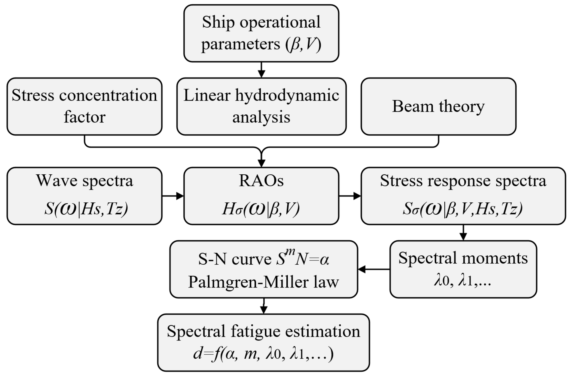
2.2. Direct Fatigue Estimation Using the Spectral Method

In addition to the rainflow counting method, Figure 1 presents a schematic workflow for a direct fatigue estimation method based on response amplitude operators (RAOs) combined with the encountered wave conditions.
The frequency domain RAOs of the structural stress response can easily be employed to obtain a ship’s short-term stress response spectrum. For fatigue assessment during a ship’s sailing life, the long-term wave conditions are assumed to comprise a series of short-term stationary sea/wave states. Each stationary sea state can last for between 30 min and 6 h. The sea states are usually described by wave statistical properties, such as the significant wave height Hs, wave period Tz, wave spectrum, and sometimes the spreading angles. Different wave spectra have been developed for such purposes. In this study, the ISSC wave spectrum [29] is used and defined as:
S ω H s ,   T z = 4 π 3 H s 2 T z 4 ω 5 exp 1 π ω T z 2 π 4 .
Finally, the ship stress response spectrum can be estimated by multiplying the square of stress RAOs with the encountered wave spectrum. However, the encountered wave spectra for certain wave frequencies can be infinite for the following sea operations, leading to unreliable stress response spectra results [30]. The stress spectral moments λ n , n = 0, 1, 2, …, can still be easily estimated by:
λ n = 0 ω + ω 2 V c o s θ g n H σ 2 ω V , θ S ω | H s , T z d ω .
If the stress signals are assumed to be a narrow-band Gaussian process for a stationary sea state of time interval T , its stress ranges follow the Rayleigh distribution. Then, the accumulated fatigue damage during this period can be approximated by the so-called NBA as follows:
    d n b = T f z α 2 3 m 2 Γ ( 1 + m 2 ) λ 0 m / 2 , a n d   f z = 1 2 π λ 2 λ 0
where fz is the frequency of zero-crossing (i.e., the frequency of stress cycles) and Γ() is the gamma function. The only variables in the above NBA are the spectral moments, which can easily be estimated by Equation (3).
However, it should be noted that the stress signals can seldom be a purely narrow-band process. Therefore, Wirsching–Light [31] proposed a correction method to increase the accuracy of fatigue damage estimation by Equation (4) and use the bandwidth parameter ε 2 to correct the NBA as follows:
d w l = ( a ( m ) + ( 1 a ( m ) ( 1 1 ε 2 2 ) b ( m ) ) d n b
where a m = 0.926 0.033 m and b m = 1.587 m 2.323 .

3. Full-Scale Measurements

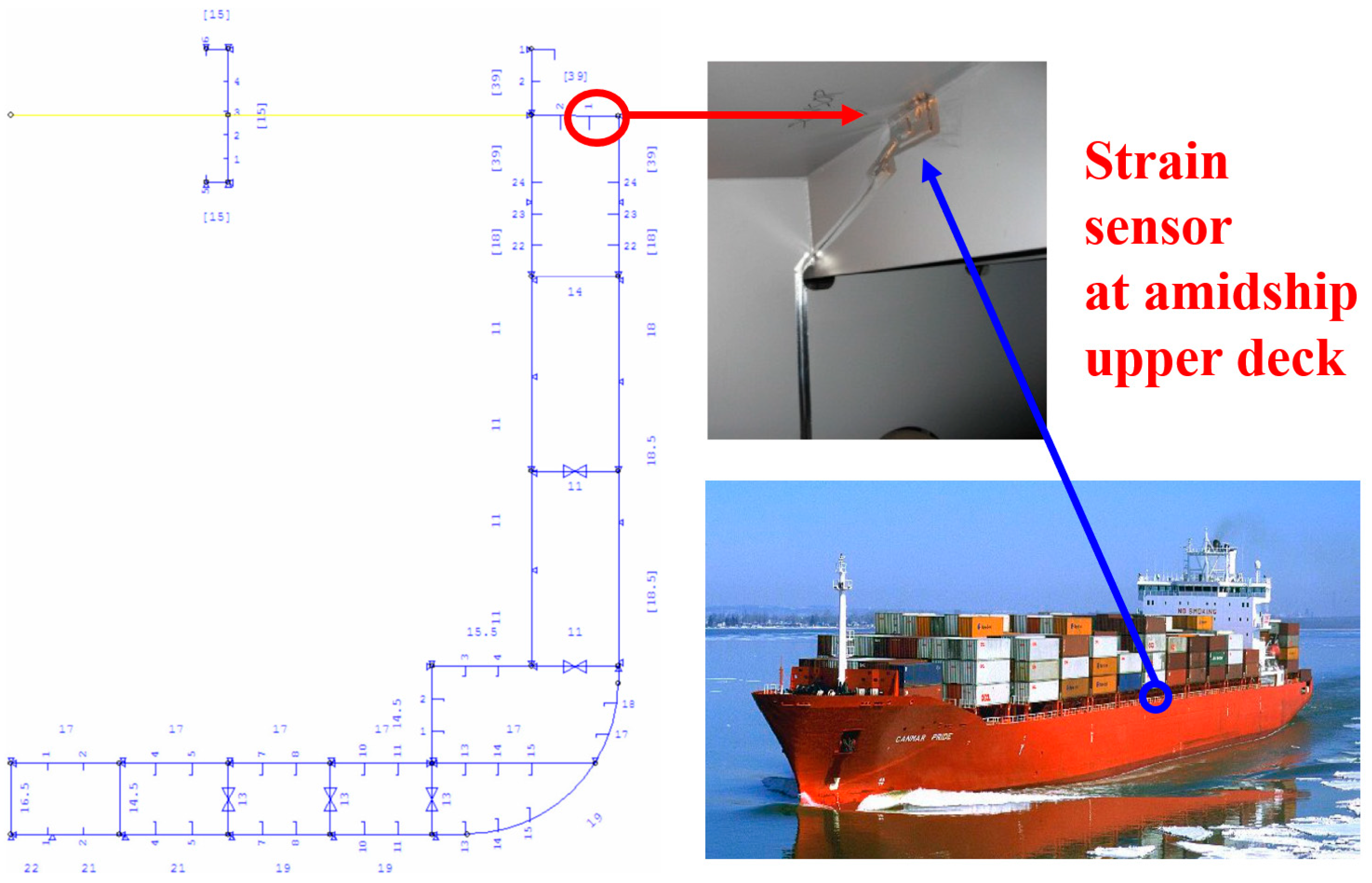
3.1. Case-Study Ship
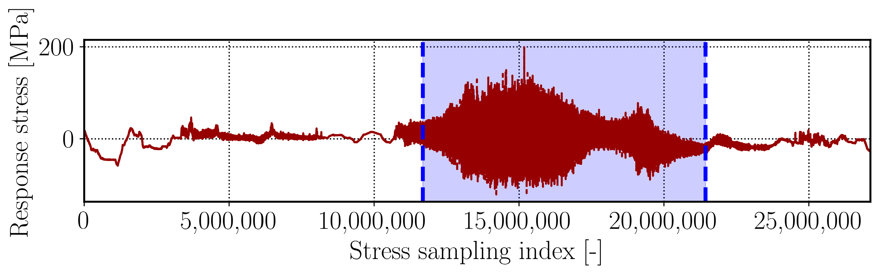
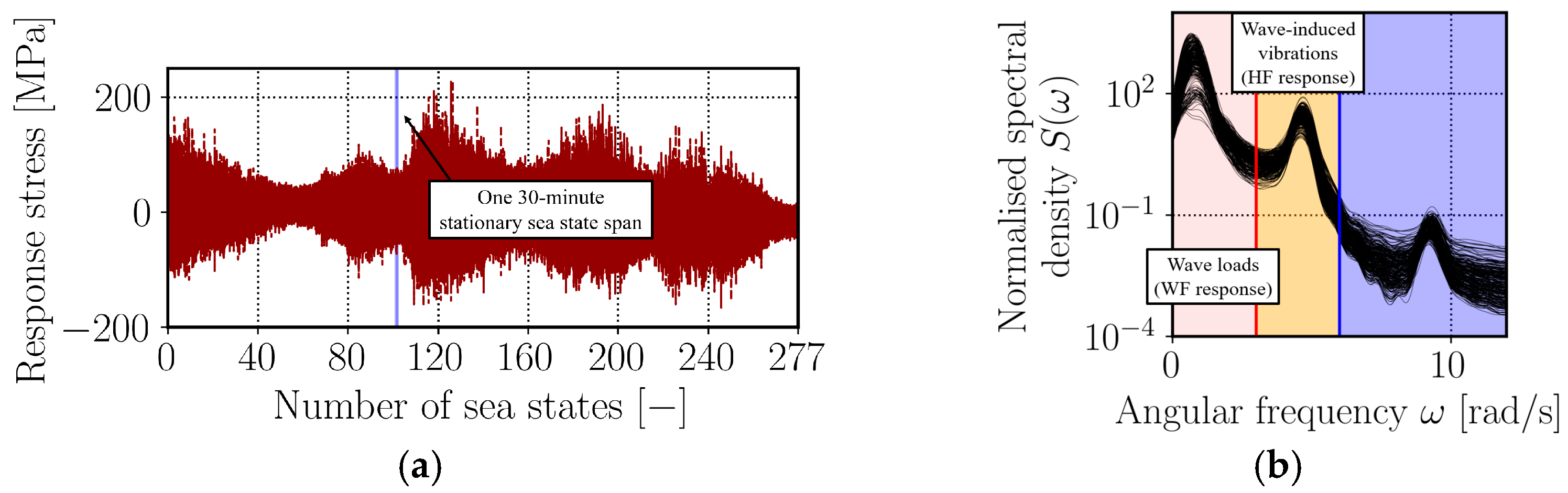
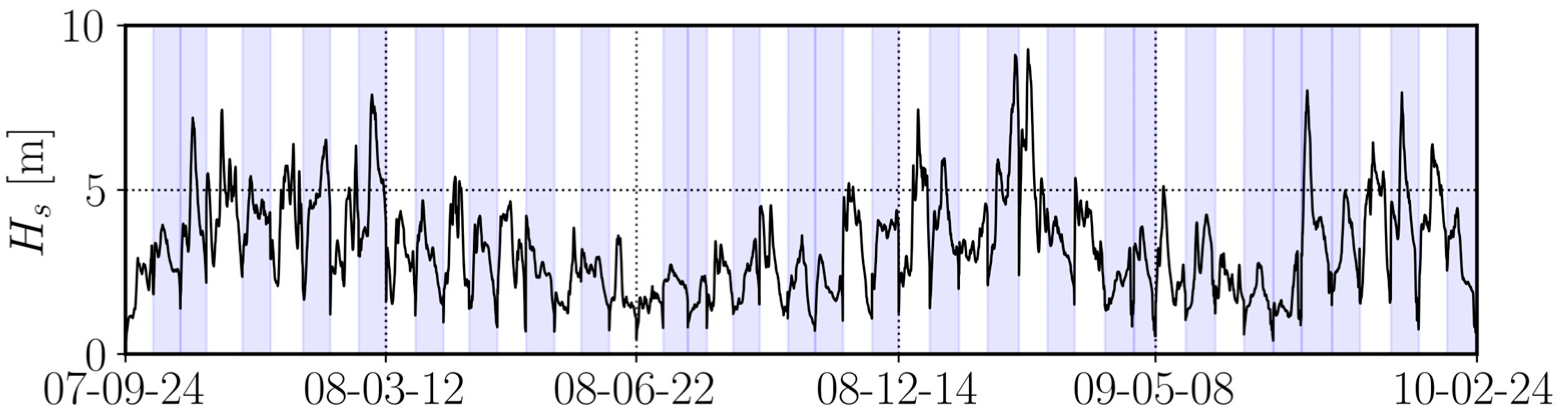
This study employed full-scale measurements from a hull monitoring system to investigate the effect of horizontal bending and torsion on a container ship’s total fatigue life. The hull monitoring system was launched in a North Atlantic sailing 2800TEU container vessel. The case-study ship was built in 1998, and its main characteristics are listed in Table 1.
The hull monitoring system followed the DNV hull monitoring rules. It recorded real-time data on GPS position (longitude and latitude), ship motion, and operational profiles (e.g., ship speed over ground and ship heading). To separate the stresses caused by torsion and bending moments, the strain sensors were arranged at different locations of the same cross-section. Four sensors in the 2800TEU container ship are located at the middle section (118.7 m from aft perpendicular (AP)) and aft section (50.3 m from AP) close to the engine room bulkhead, respectively. The sensors are placed on the stiffener web and measure the nominal longitudinal strain of both the port and starboard sides. The sensor on the starboard side amidships is shown in Figure 2.
In this study, only the vertical bending-induced normal stress at the middle section was applied for the fatigue analysis. Thus, the considered stress values were the average of stress measured on the port and starboard sides. A motion response unit (MRU) was also installed at the central line and measured the container vessel’s 6 DOF motions. The MRU measurements include 16 variables: motion Z = [ z 2 , z 3 , z 4 , z 5 , z 6 ] , motion velocity Z ˙ = [ z ˙ 2 , z ˙ 3 , z ˙ 4 , z ˙ 5 , z ˙ 6 ] , and motion acceleration Z ¨ = [ z ¨ 1 , z ¨ 2 , z ¨ 3 , z ¨ 4 , z ¨ 5 , z ¨ 6 ] . For these variables, z 1 to z 6 denote surge, heave, sway, roll, yaw, and pitch, respectively.
The case-study ship operates the trade between Western Europe and Quebec in Canada. A total of 48 complete sailing voyages from September 2007 to February 2010 were selected from the full-scale measurements and applied in fatigue modeling and analysis. This study did not include the other voyages missing more than 50% of measurements. The measurement frequency of strain/stress and ship motions was 25 Hz, and the frequency for other operational parameters was 1 Hz.
The North Atlantic is considered one of the world’s harshest sea environments. Especially during winter, more low-pressure systems are expected for every cross-Atlantic voyage, and 15~25% of the significant wave height encountered is larger than 5 m [11]. All 48 case-study voyages are presented in Figure 3 for winter and summer sailing, respectively.
As shown in Figure 3a, the container vessel chose alternative routes that deviated notably from the shortest route to avoid heavy weather during winter navigations. Since the focus of the present study was on the open sea area, the measurements close to coasts and in shallow water areas were excluded by two spatial boundaries (i.e., 55 °   W and 5 °   W longitude), as indicated by the red vertical line in Figure 3. The applied spatial boundaries also resulted in the abnormal stress samples in ports and coastal areas being disregarded. Figure 4 presents one voyage example of the response stress (25 Hz) for the 24 April 2008 voyage. The blue frame is the spatial boundaries’ selected span, and the stresses’ mean value is set to 0. It is clearly shown that the applied span only consists of the stress induced during normal navigation. The low-fluctuation stress during anchor/drifting or calm water sailing near the berth was excluded.

3.2. Data Analysis

This study assumed a stationary sea state to be 30 min. After data synchronization and geographic boundary filtering for deep-sea conditions, the final applied sample size for fatigue machine learning modeling was 10,377.
For the i-th 30-min stationary sea state, the fatigue damage accumulation d i was calculated using the rainflow count method based on stress measurements. In addition to the ship stress response caused by wave-induced hydrodynamic loads, container vessels also need to consider two other wave-induced vibrations: springing and whipping. The springing response is a resonant hull girder response that depends on the structural dynamics and wave frequencies. Large and frequent slamming loads excite the transient vibratory response (i.e., whipping of the vessel). Figure 5 presents the normalized stress spectra ( λ 0 = 1 ) using the Fourier transformation to transfer the response into the power spectral density based on the stress measurements of the 2800TEU container ship’s first westbound winter voyage in 2008. After geographic boundary filtering, the 6 January 2008 voyage included 277 stationary sea states, while the blue frame in Figure 5a indicates the 150th 30-min sea state.
In Figure 5b, the typical multi-peak character of the spectra can be observed from the 277 investigated spectra. The first spectral peak is related to the wave frequency load-induced ship responses, while the second peak is caused by the ship whipping and springing. Here, the wave-induced hydrodynamic loads (main ship responses) are denoted as WF responses, while the wave-induced vibrations (whipping and springing) are denoted as the high-frequency (HF) responses. In this study, not only the damage d W F caused by the WF responses but also the damage d T F due to the total frequency (TF = WF + HF) loads were considered. The WF response was extracted from the total response by a Fourier analysis with a frequency range of 0 to 3 rad/s, while the frequency of TF was 0 to 6 rad/s.
For each stationary sea state, the statistics of the 16 motion variables were extracted based on the 30-min window measurement signals. The statistics consist of the mean value, standard deviation, skewness, and kurtosis. The motion acceleration Z ¨ measurements within the 150th sea state window in Figure 5a are depicted in Figure 6. The solid line is the mean value, while the dashed lines are the one-time standard deviation boundaries of Z ¨ . The mean values of all motion accelerations Z ¨ within this 30-min interval are approximately 0 (see Figure 6). This indicates that the mean value may not determine the fatigue estimation. The correlation analysis is presented in Section 4, which involved selecting input features for fatigue machine learning modeling.
The encountered metocean environments (i.e., mean wave direction D w a v e , mean wave period T z , and significant wave height H s ) were extracted from the ERA5 reanalysis dataset hourly with 0.5 ° × 0.5 ° spatial resolution [32]. The current velocities U c u r r e n t and V c u r r e n t were obtained from the Copernicus Marine Service with 0.083 ° × 0.083 ° geographical resolution and a temporal resolution of 24 h [33]. The ship’s speed through the water was then estimated by the measured speed over ground and current conditions, following the ISO guidelines [34].

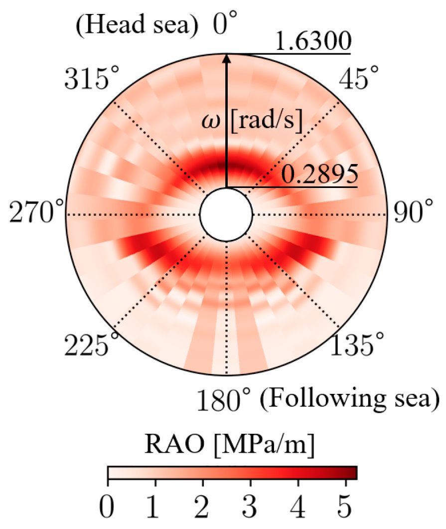
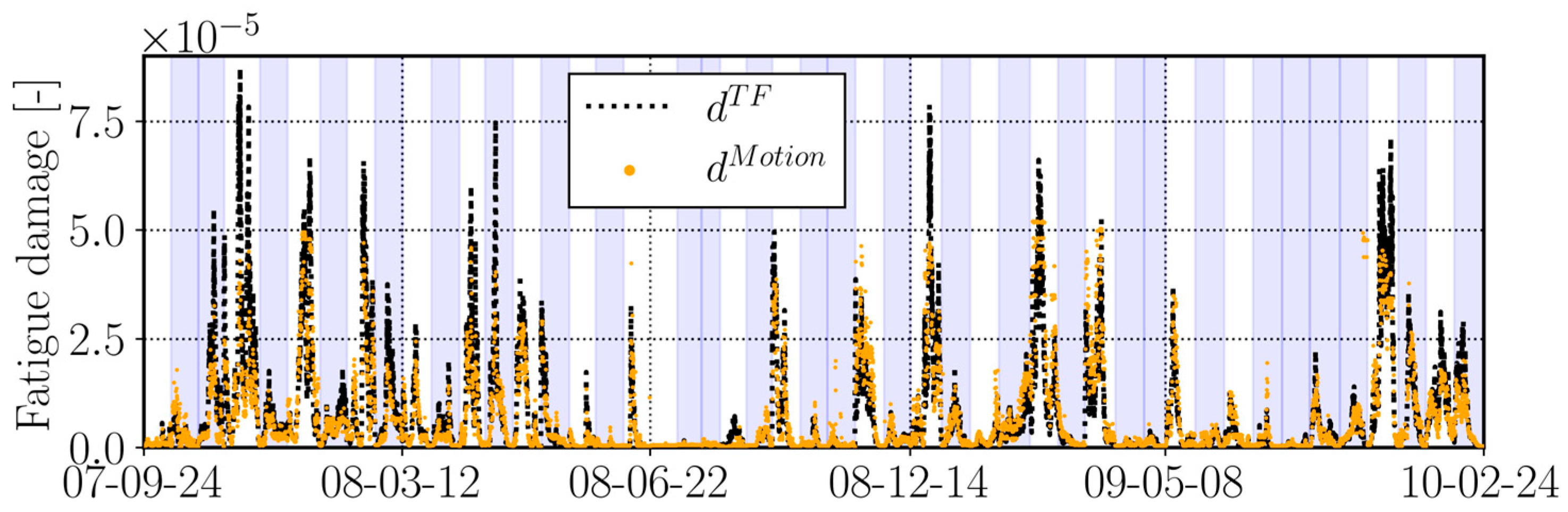
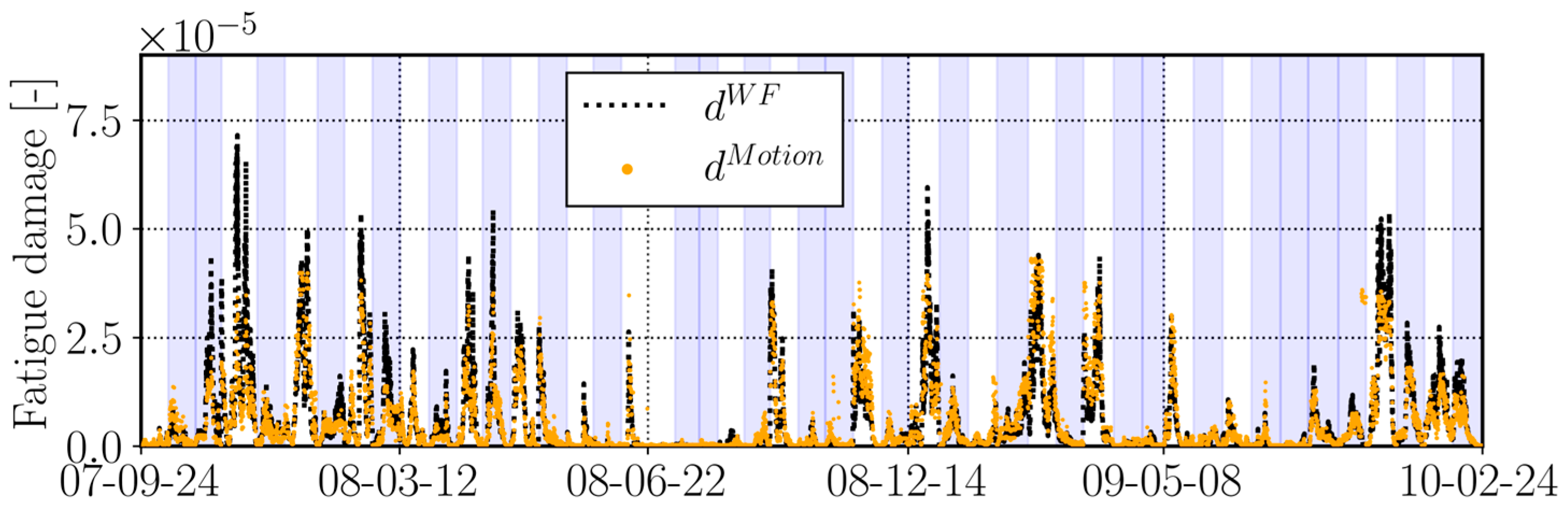
3.3. Rainflow Count Fatigue Damage and RAOs for Spectral Methods

The fatigue damage along the 30-min stationary sea states for the 48 voyages was estimated using the rainflow count method based on the measured stresses. The TF load-induced damage d T F and wave frequency load-induced damage d W F are presented in sailing sequence (i.e., from September 2007 to February 2010) in Figure 7. The white and blue frames represent westbound and eastbound voyages, respectively. As shown in Figure 7, the more considerable fatigue damage mainly occurs in the winter sailing westbound voyages because the weather encountered during winter is harsher and larger waves occur. Since storms in the North Atlantic always blow from west to east, the relative wave angle of westbound sailing is rather stable close to the head sea. The TF load-induced fatigue damages d T F are always larger than the d W F since the latter does not consider the HF response-induced fatigue damage caused by whipping and springing. Additionally, the differences d T F d W F are more obvious when the weather conditions are worse because larger waves will excite more significant vibrations, causing HF responses to contribute more fatigue damage.
The case-study container vessel’s RAOs were obtained by first evaluating wave bending moments using a hydrodynamic analysis based on a 2D potential theory and a ship model with 20 strips [35]. The fully loaded condition was considered in the hydrodynamic analysis to determine the wave loads applied to the hull of this container ship. The global stresses on the hull girder were then estimated using the beam theory. The RAOs of the local stresses were computed by multiplying the girder stresses by a stress concentration factor (SCF), which is considered 2 for this container vessel. Figure 8 presents the RAO polar heatmap for one example speed (i.e., V = 12 m/s).
The angle of the polar diagram is the relative wave angle θ , while the radius is the wave frequency ω (ranging from 0.2895 to 1.63 rad/s). The color of the heatmap represents the RAO values; the darker the color, the greater the value of H σ ( ω | V , θ ) and the larger the stress response in the same H s and T z condition.

4. Machine Learning Model Establishment
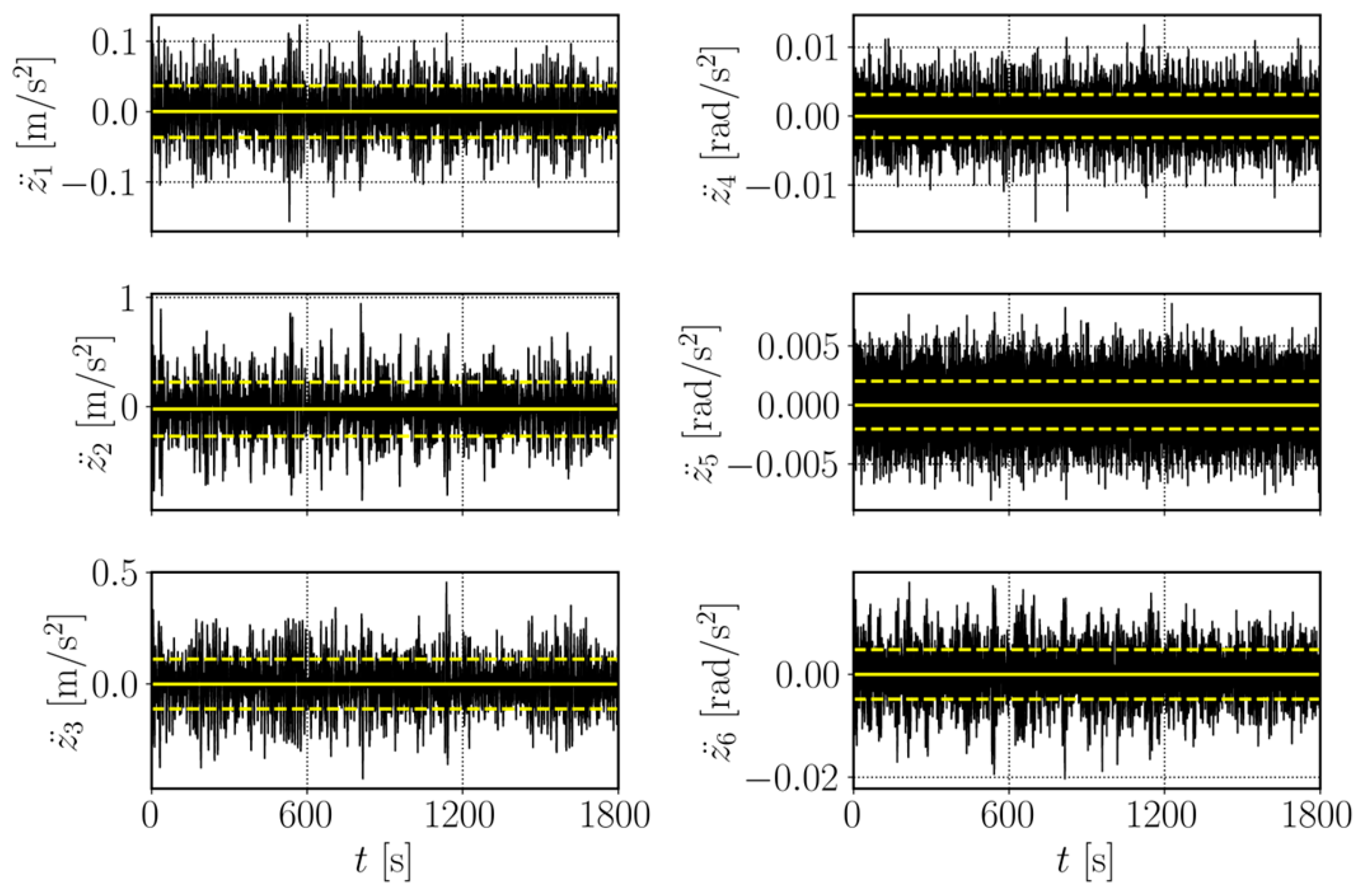
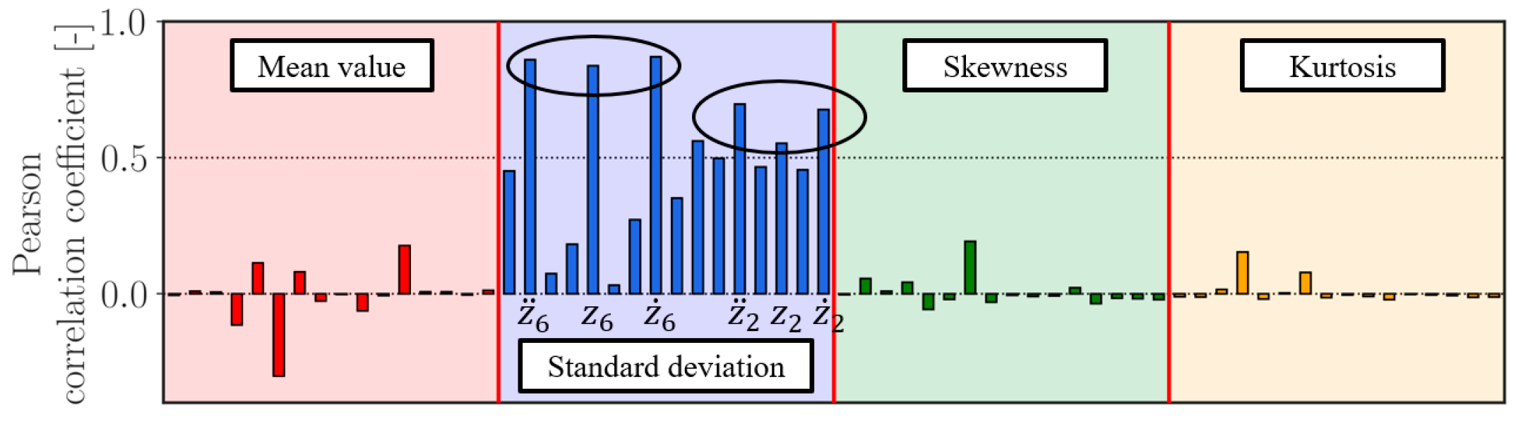
4.1. Input Features

The machine learning model was established to describe a ship’s fatigue damage accumulated during a sea state in terms of the input features (denoted as X _ ¯ ). The prediction target is the observed ship fatigue damage in the assumed stationary 30-min sea states (i.e., D = [ d 1 , d 2 d n ] ), where n is the sample size. The observed fatigue damage was estimated using the rainflow count method for each 30-min stress signal.
As discussed in Section 3, the mean value, standard deviation, skewness, and kurtosis of the 16 MRU measured variables were extracted from each 30-min stationary sea state. Therefore, a total of 16 × 4 features could be chosen for the ship motion-based fatigue machine learning modeling. However, if the average values are around 0 (as shown in Figure 6), then the correlation between the average value of motion and fatigue damage is not high. To reduce the dimension of the features, the Pearson correlation coefficients of different statistics relative to fatigue damage were calculated and are compared in the histogram presented in Figure 9. Here, the fatigue damage is d T F due to the total frequency (TF = WF+HF) loads, and the Pearson correlation coefficients relative to d W F are similar.
The standard deviations of Z , Z ˙ , and Z ¨ have the highest correlation with fatigue damage d T F . Among them, as marked in Figure 9, the correlation coefficient of the pitch-related measurements’ ( z 6 , z ˙ 6 , z ¨ 6 ) standard deviation exceeds 0.8, while the standard deviation’s correlation coefficient of the heave motions ( z 2 , z ˙ 2 , z ¨ 2 ) are also relatively high (~0.6). The motion’s mean value, skewness, and kurtosis have rather small correlation coefficients and are not strongly correlated to fatigue damage (even negative correlation). Therefore, for the ship motion-based machine learning model, the applied input features are X _ ¯ = [ v a r ( z 6 ) , v a r ( z ˙ 6 ) , v a r ( z ¨ 6 ) , v a r ( z 2 ) , v a r ( z ˙ 2 ) , v a r ( z ¨ 2 ) ] pitch- and heave-related variables.

4.2. XGBoost Algorithm

This study used the eXtreme gradient boosting (XGBoost) algorithm for modeling machine learning. XGBoost is a type of gradient tree boosting method [36]. Each weak evaluator in XGBoost is a tree. The applied XGBoost algorithm aimed to establish the relationship between the prediction target (i.e., the rainflow count fatigue damage d i ) and the input features. Assuming that the ensemble model has a total number of K decision trees, the prediction for this i -th sample d i ^ is:
d i ^ = k = 1 K f k X _ ¯ i ,             i = 1 , , n  
where n is the total number of training samples and f k is the k -th decision tree. Standard objective functions (e.g., error rate, mean square error, etc.) can only evaluate the performance of a model and cannot assess its computing efficiency. The objective function of XGBoost, which includes model complexity to quantify efficiency, is defined as follows:
  O b j = i = 1 n l d i , d i ^ + k = 1 K Ω f k
where the first component is the conventional loss function, which quantifies the residual between the actual damage d i and the predicted values d i ^ —often the root-mean-square error (RMSE). The second component indicates the model complexity, which is measured based on the structure of the tree. More details regarding the XGBoost algorithm and the hyperparameters are provided in [37].

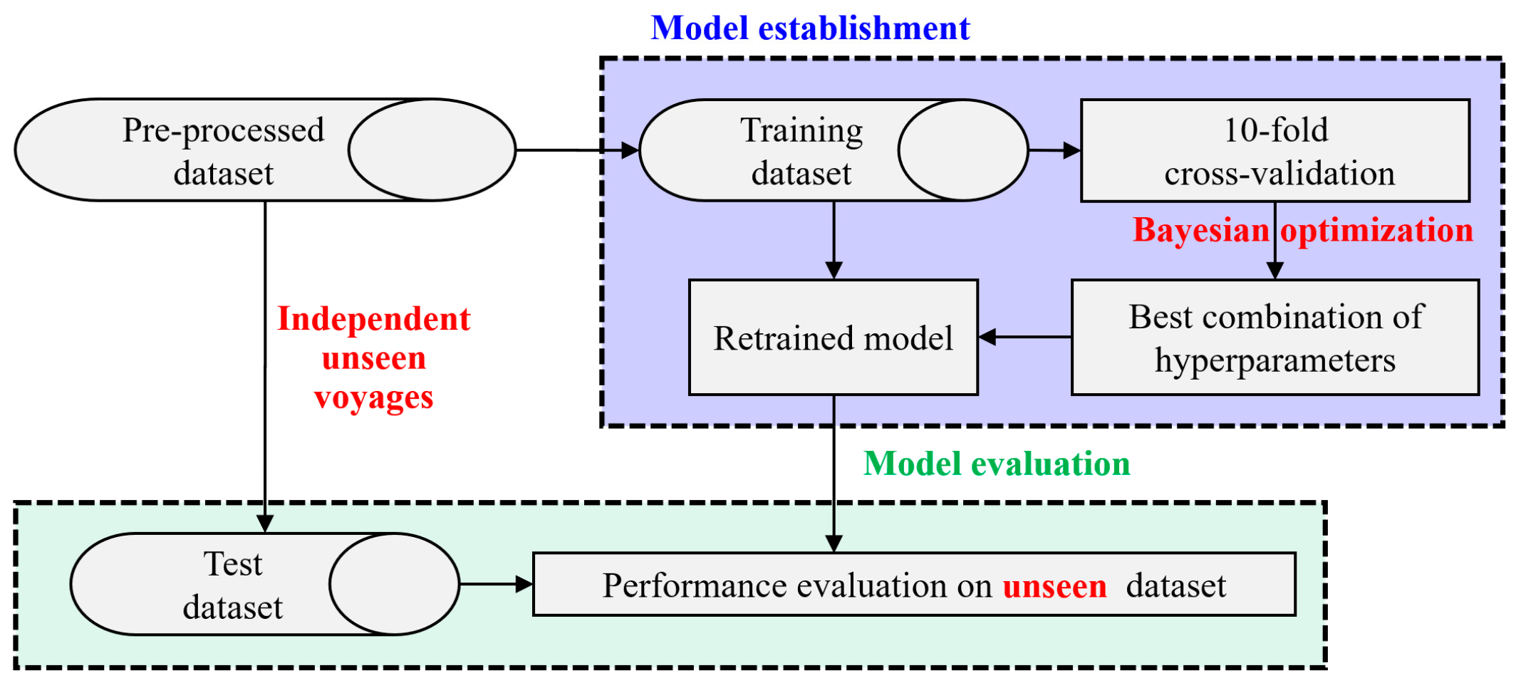
4.3. Model Establishment

The workflow for establishing the fatigue machine learning model is presented in Figure 10. The test set is each independent voyage shown in Figure 3, held out from the pre-processed dataset for unseen data evaluation. The rest of the dataset was split into a training set to establish the model.
Bayesian optimization was used to determine the optimal hyperparameters of the XGBoost modeling, which was widely used in machine learning for hyperparameter tuning. Bayesian optimization is a method that uses the Bayesian theorem to create adaptive data for hyperparameters and uses surrogate models to determine the best values for the hyperparameters. The 10-fold cross-validation procedure prevents model overfitting and ensures that the selected hyperparameter combination values are close to the ideal values, while the RMSE is applied as the validation metric. The specific hyperparameters applied, as well as their respective tuning ranges, are presented in Table 2.

5. Results and Discussion

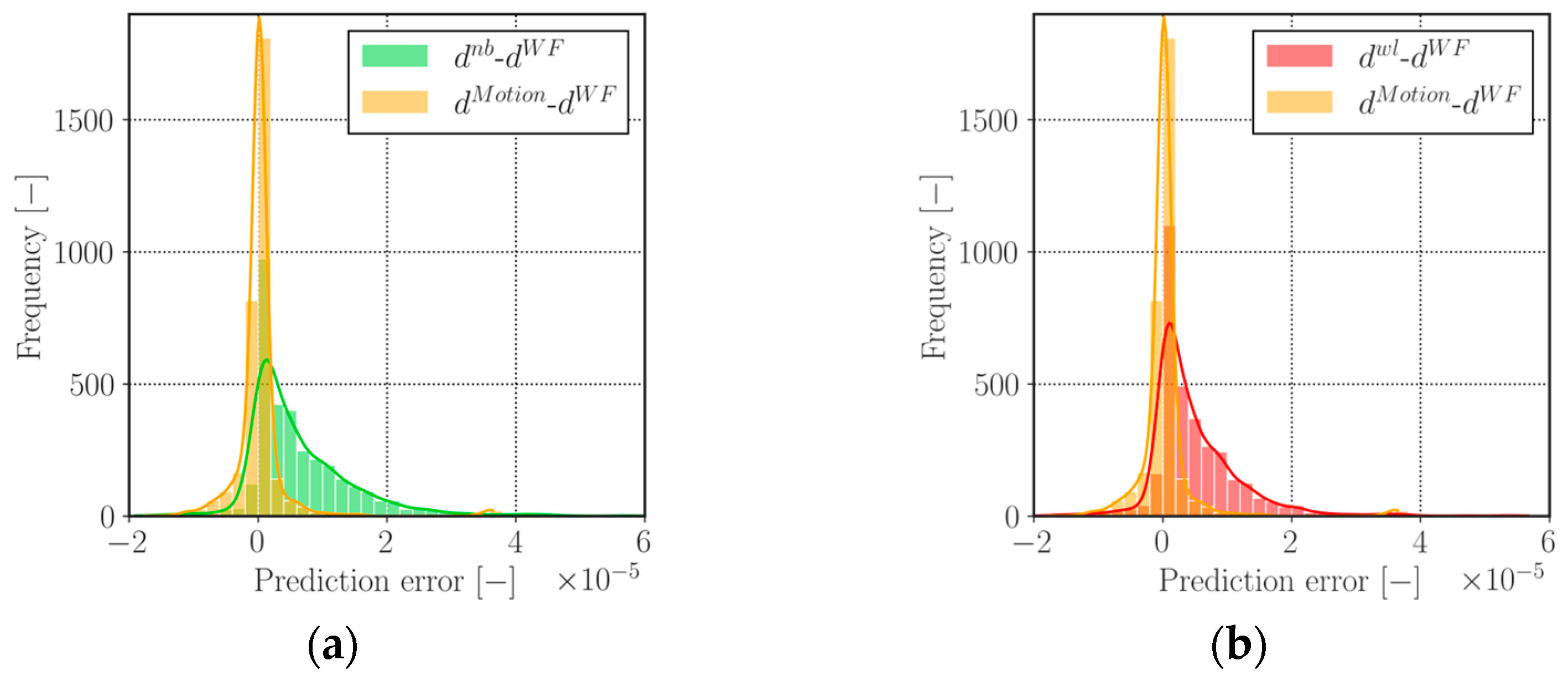
5.1. Fatigue Prediction Uncertainties of Spectral Methods Based on RAOs

The spectral fatigue assessment methods introduced in Section 2 were first employed to evaluate the fatigue damage. This study did not employ the correction methods to split the stress response spectrum for the spectral method; therefore, the spectral approaches were only used to investigate wave frequency load-induced fatigue d W F .
The rainflow counting fatigue damage d W F in the time series, as well as d n b and d w l , predicted by narrow-band and Wirsching–Light approximation, are presented in Figure 11. The encountered significant wave height H s along the sailing route is also shown in Figure 12.
As illustrated in Figure 11, the spectral methods significantly overestimated the fatigue damage when compared to the values obtained using the rainflow count method. This overestimation is particularly pronounced for winter voyages, where wave conditions are harsher (see Figure 12). This discrepancy escalates with increasing wave height, indicating that traditional spectral methods tend to yield higher calculations of fatigue damage under such conditions. Conversely, these methods only provide relatively accurate estimations for westbound sailing in calm sea conditions. This discrepancy underscores the inherent limitation of spectral methods based on wave spectrum in effectively capturing the real-world non-linear impact of wave height on fatigue damage. However, among the two spectral methods examined, the Wirsching–Light method, which integrates the bandwidth parameter, demonstrates a relatively lower level of overestimation than the original narrow-band method.

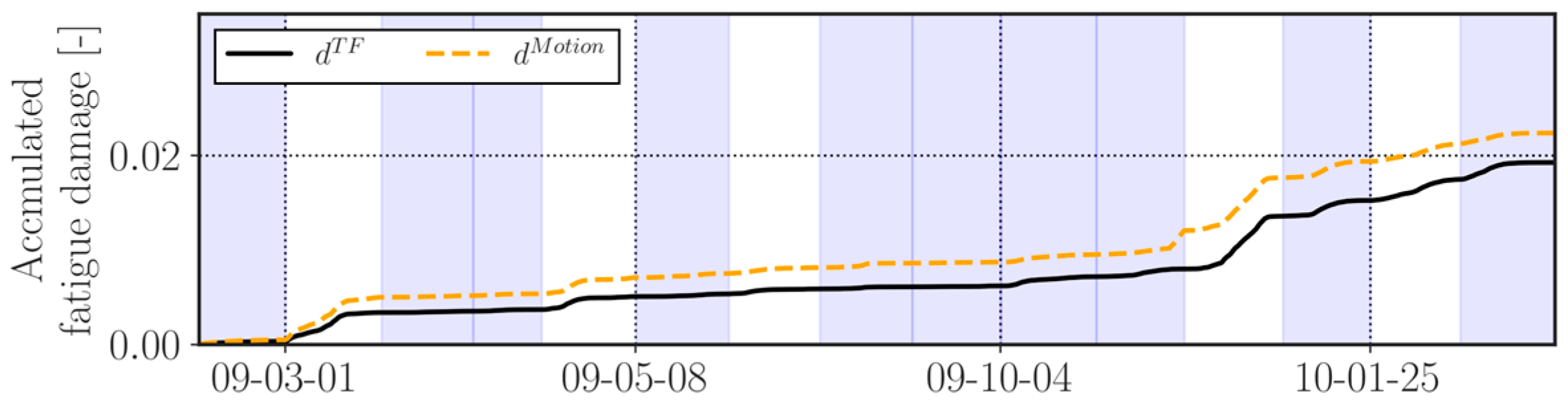
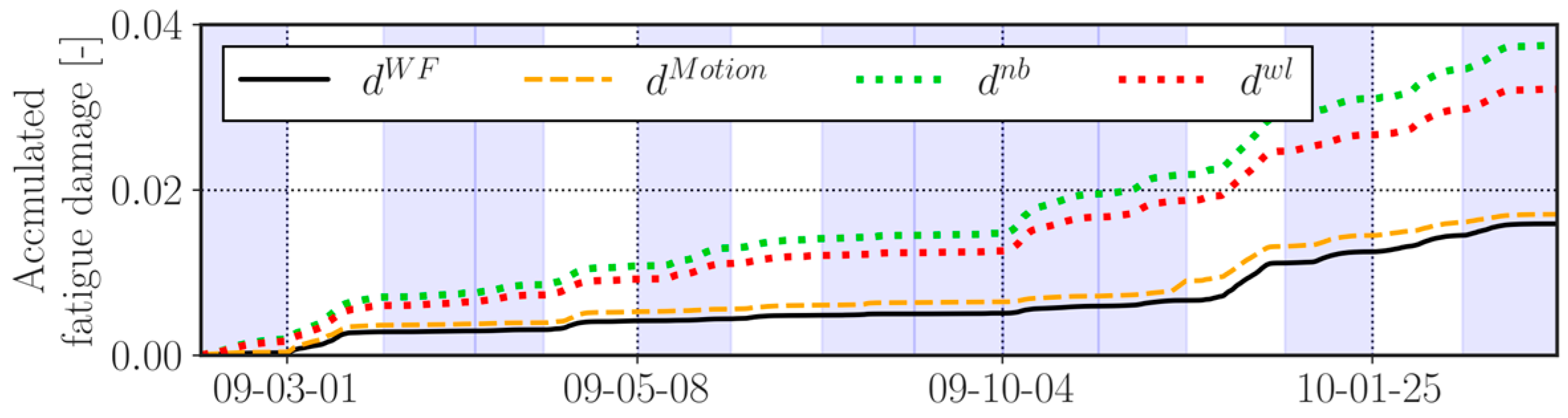
5.2. Fatigue Prediction by Proposed Machine Learning Model Based on Heave and Pitch Motions

Subsequently, the ability of the motion-based machine learning model to predict fatigue damage was evaluated across 48 distinct routes in a case study. Specifically, each voyage was treated as an individual, unseen test case, while the machine learning model was trained on the remaining 47 routes constituting the training set. Upon determining the optimal combination of hyperparameters through Bayesian optimization on the training set, the machine learning models were established 48 times, each corresponding to a unique voyage. Figure 13 and Figure 14 depict the machine learning model’s predictive results on the test set for different voyages, which are presented in chronological sequence. Figure 13 presents the prediction results for TF load-induced fatigue d T F , whereas Figure 14 focuses on the fatigue d W F induced by wave frequency load.
According to Figure 13 and Figure 14, the proposed machine learning model demonstrates a commendable ability to follow the fatigue damage calculations as determined by the rainflow count method, which are applicable to both TF load-induced fatigue and wave frequency load-induced fatigue. In these figures, regardless of whether the voyages occurred in winter with harsh sea conditions or in summer with calmer waves, the machine learning model does not exhibit the severe overestimation characteristic of traditional spectral methods as observed in Figure 11. This indicates that a model based on heave and pitch motions, coupled with actual sea state conditions, can effectively overcome the uncertainties inherent in traditional methods and sea spectrum modeling. Consequently, it offers a more accurate prediction of fatigue damage for ships operating in real-world sea conditions. However, specifically regarding the proposed machine learning model, its predictions for fatigue d W F induced by wave frequency load are marginally more accurate, particularly in high wave conditions where underestimation is not as severe as in the case of total frequency load-induced fatigue d T F . This indirectly demonstrates that HF wave loads (e.g., whipping and springing) reduce the performance of the machine learning model.

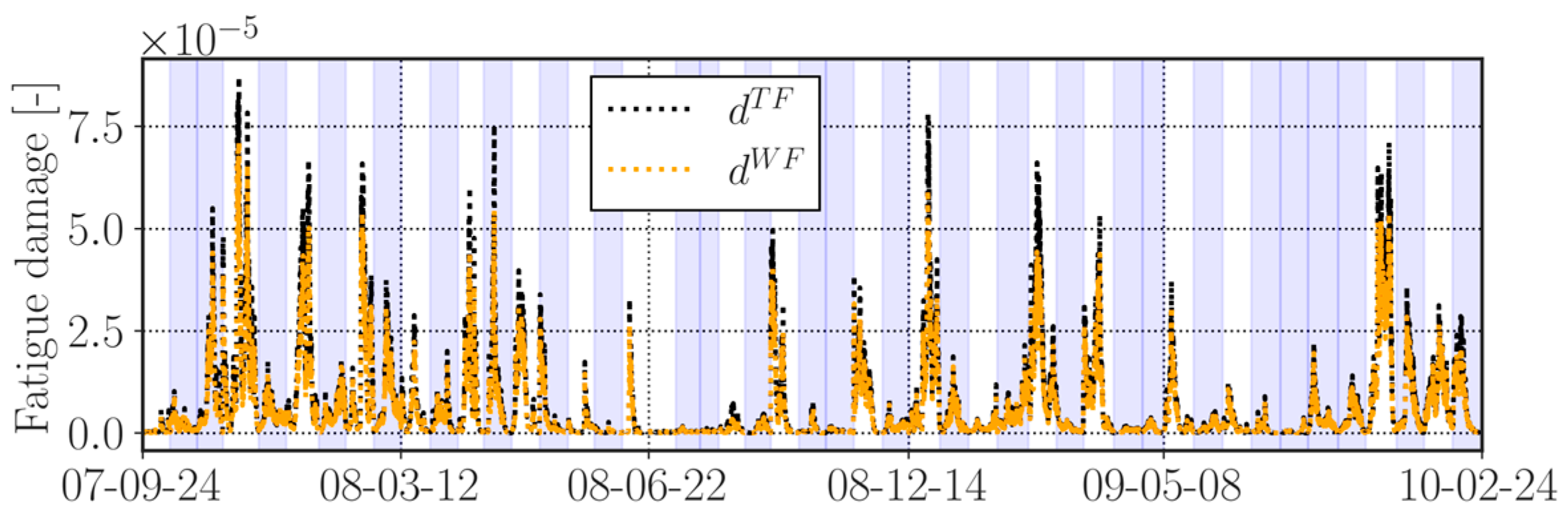
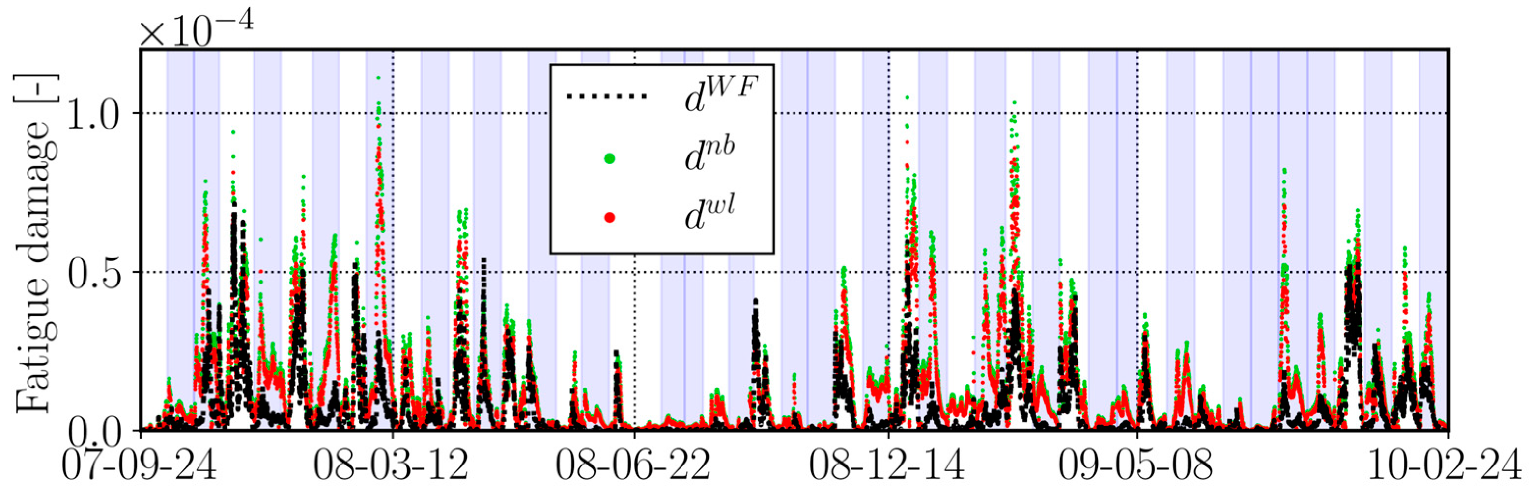
5.3. Fatigue Prediction Ability Evaluation for Long-Term Unseen Voyages

Except for each unseen voyage as a test set, the fatigue assessment model should be able to predict and monitor the fatigue for a period of time in the future or the entire life cycle of the ship. In this part, the 33 voyages before February 2009 were applied as the training set, while the remainder (approximately 30%) of the dataset (i.e., 15 complete unseen voyages from February 2009 to February 2010 (1 year)) was used as the test set. This split is more in line with the needs of the shipping industry, which uses past data and recent weather condition forecasts to optimize a ship’s operation.
The final year’s 15-voyage selection was not solely based on the data split method that matched the 70% training and 30% test sets most commonly used by the machine learning community. Moreover, as seen in Figure 12, the pre-February 2009 sailing data covered a range from calm sea conditions to harsh conditions with H s of more than 9 m. Even if many wave heights exceed 5 or even 8 m in the subsequent test set voyages, a machine learning model based on the previous training data will give robust predictions.
Based on the 1-year unseen voyage data, the fatigue prediction capabilities of the proposed machine learning model and traditional spectral methods for long-term unseen voyages were evaluated and compared. The distribution of prediction errors between the machine learning model and observed data is depicted in Figure 15. For comparison, Figure 15a also presents the distribution of prediction errors between the narrow-band method and observed data, while Figure 15b displays the distribution of prediction errors for the Wirsching–Light approximation compared to observations. As illustrated, the prediction error distributions for both spectral methods are skewed to the right of zero, indicating a pronounced overestimation that is consistent with the observations shown in Figure 11. In contrast, the prediction errors of the machine learning model are more uniformly distributed across both the positive and negative sides of zero, exhibiting no significant overestimation or underestimation. This suggests that for long-term monitoring of cumulative ship fatigue, the estimated accumulated fatigue damage by the machine learning model is likely to be more accurate than that predicted by spectral methods.
Building on the aforementioned analysis, the machine learning model and spectral methods’ predictions of fatigue damage accumulation for the 1-year unseen voyages were compared with observed values in a chronological sequence. Figure 16 compares the cumulative fatigue damage d T F induced by TF loads and the machine learning model’s predictions, d M o t i o n . During the 15 cross-Atlantic navigations, the fatigue damage had accumulated to approximately 0.019 by the end of February 2010. While the machine learning model captured the overall trend compared to the observations, the cumulative error in over-prediction was approximately 16%. Subsequently, Figure 17 illustrates the cumulative fatigue damage d W F induced by wave frequency load by comparing the machine learning model’s and spectral methods’ predictions. As observed in Figure 11 and Figure 15, both the narrow-band ( d n b ) and Wirsching–Light ( d w l ) approximation methods exhibited significant overpredictions, resulting in cumulative errors of approximately 100 and 90%, respectively, by February 2010. In contrast, the machine learning model’s predictions for wave frequency load-induced fatigue damage, which were not influenced by HF stress caused by wave-induced vibration (whipping and springing), were largely consistent with the actual measurements. This aligns with the analysis presented in Figure 15, where the machine learning model’s prediction errors were uniformly distributed across both the positive and negative sides of zero, leading to a relatively minimal cumulative error.

6. Conclusions

The study applied machine learning techniques to predict a North-Atlantic-sailing 2800TEU container vessel’s fatigue damage based on the full-scale measurement data of the onboard hull monitoring system. The recorded ship’s heave and pitch motion responses, as well as the related motion velocity and acceleration, were deployed as input features. The modeling targets were wave frequency load-induced fatigue damage d W F , as well as the TF load-induced fatigue damage d T F considering HF whipping and springing. Based on the comparison of the test set of individual unseen voyages, the proposed machine learning model achieved much better predictive ability than the widely used spectral methods for direct fatigue calculation. This is because the traditional spectral methods are unable to accurately capture the nonlinear increase in fatigue damage that occurs with increasingly harsh sea conditions. Additionally, there are inherent deviations and uncertainties when employing a wave spectrum to describe actual sea environments. The proposed models were also applied for long-term unseen voyage evaluation. The machine learning model still provided satisfactory predictions for nearly 1 year of unseen sailing data. Especially for wave-induced fatigue damage, the prediction is nearly consistent with the observation d W F . It was also found that HF whipping and springing introduced uncertainties and noise into the model establishment. The machine learning model’s predictive ability for d W F was slightly better than that for d T F .
This work equips the maritime transportation industry with tools and methodologies for evaluating ship fatigue safety performance. For instance, shipping companies can utilize these methods for the more precise monitoring of fatigue damage. Additionally, shipping operators can enhance their operational safety by integrating the proposed machine learning model into their voyage optimization systems. This integration facilitates route planning that strategically avoids severe fatigue damage accumulation by optimizing ship speed and routing to evade harsh maritime environments. Such advancements can lead to reduced maintenance requirements, potentially extending the service life of vessels and enhancing the safety of onboard crew and cargo.
Furthermore, the calculation of fatigue damage in this study—based on measured stress—was conducted based on the linear Palmgren–Miner’s law while utilizing a specific S-N curve in conjunction with the rainflow counting method. Palmgren–Miner’s law is frequently recommended and applied in ship fatigue calculations due to its widespread acceptance and user-friendly nature. However, it is critical to acknowledge the limitations inherent in this method. Notably, future research may benefit from the implementation of more sophisticated and physically based constitutive models for the more nuanced modeling of fatigue.

Author Contributions

Conceptualization, X.L., D.W. and W.M.; methodology, X.L. and C.Z.; software, X.L.; validation, X.L. and W.T.; formal analysis, X.L. and D.W.; investigation, X.L. and W.T.; writing—original draft preparation, X.L. and D.W.; writing—review and editing, X.L., J.W.R. and W.M.; visualization, X.L. and C.Z.; supervision, J.W.R. and W.M.; project administration, W.M.; funding acquisition, D.W. and W.M. All authors have read and agreed to the published version of the manuscript.

Funding

This research was funded by the Swedish Transport Administration (project TRV2019/119989), Vinnova (project 2021-02768), Swedish Foundation for International Cooperation in Research and Higher Education (CH2016-6673), and Fundamental Research Funds for the Central Universities (WUT:2022IVA139, WUT:223144002).

Institutional Review Board Statement

Not applicable.

Informed Consent Statement

Not applicable.

Data Availability Statement

The dataset is not publicly available due to confidentiality agreements with the data provider.

Acknowledgments

The authors acknowledge ship owners for providing full-scale measurement data.

Conflicts of Interest

The authors declare no conflict of interest. The funders had no role in the design of the study, in the collection, analyses, or interpretation of data, in the writing of the manuscript, or in the decision to publish the results.

References

  1. Rychlik, I. A new definition of the rainflow cycle counting method. Int. J. Fatigue 1987, 9, 119–121. [Google Scholar] [CrossRef]
  2. Rychlik, I. Note of cycle counts in irregular loads. Fatigue Fract. Eng. Mater. Struct. 1993, 16, 377–390. [Google Scholar] [CrossRef]
  3. Li, Z.; Mao, W.; Ringsberg, J.W.; Johnson, E.; Storhaug, G. A comparative study of fatigue assessments of container ship structures using various direct calculation approaches. Ocean Eng. 2014, 82, 65–74. [Google Scholar] [CrossRef]
  4. Yang, P.; Li, J.; Zhang, W.; Wu, D.; Gu, X.; Ma, Q. Analysis on statistical uncertainties of wave loads and structural fatigue reliability for a semi-submersible platform. Ocean Eng. 2021, 237, 109609. [Google Scholar] [CrossRef]
  5. Yosri, A.; Leheta, H.; Saad-Eldeen, S.; Zayed, A. Accumulated fatigue damage assessment of side structural details in a double hull tanker based on spectral fatigue analysis approach. Ocean Eng. 2022, 251, 111069. [Google Scholar] [CrossRef]
  6. Mao, W. Development of a spectral method and a statistical wave model for crack propagation prediction in ship structures. J. Ship Res. 2014, 58, 106–116. [Google Scholar] [CrossRef]
  7. Lang, X.; Wang, H.; Mao, W.; Osawa, N. Impact of ship operations aided by voyage optimization on a ship’s fatigue assessment. J. Mar. Sci. Technol. 2020, 26, 750–771. [Google Scholar] [CrossRef]
  8. Gaidai, O.; Storhaug, G.; Naess, A.; Ye, R.; Cheng, Y.; Xu, X. Efficient fatigue assessment of ship structural details. Ships Offshore Struct. 2019, 15, 1–8. [Google Scholar] [CrossRef]
  9. Thompson, I. Fatigue damage variation within a class of naval ships. Ocean Eng. 2018, 165, 123–130. [Google Scholar] [CrossRef]
  10. Yamamoto, N. Fatigue evaluation of ship structures considering change in mean stress condition. Weld. World 2017, 61, 987–995. [Google Scholar] [CrossRef]
  11. Mao, W. Fatigue Assessment and Extreme Prediction of Ship Structures. PhD Thesis, Chalmers University of Technology, Gothenburg, Sweden, 2010. [Google Scholar]
  12. Jordan, C.R.; Cochran, C.S. In-service performance of structural details. In Ship Structure Committee; Report SSC-272; US Coast Guard: Washington, DC, USA, 1978. [Google Scholar]
  13. Jordan, C.R.; Knight, L.T. Further survey of in-service performance of structural details. In Ship Structure Committee; Report SSC-294; US Coast Guard: Washington, DC, USA, 1978. [Google Scholar]
  14. Fricke, W. Fatigue and fracture of ship structures. In Encyclopedia of Maritime and Offshore Engineering; John Wiley & Sons, Ltd.: New York, NY, USA, 2017; pp. 1–12. [Google Scholar]
  15. Storhaug, G.; Moe, E.; Piedras Lopes, T.A. Whipping measurements onboard a midsize container vessel operating in the North Atlantic. In Proceedings of the International Symposium on Ship Design and Construction, Marintec, Shanghai, China, 27-30 November 2007; pp. 55–70. [Google Scholar]
  16. Zhang, M.; Kujala, P.; Musharraf, M.; Zhang, J.; Hirdaris, S. A machine learning method for the prediction of ship motion trajectories in real operational conditions. Ocean Eng. 2023, 283, 114905. [Google Scholar] [CrossRef]
  17. Gupta, P.; Rasheed, A.; Steen, S. Ship performance monitoring using machine-learning. Ocean Eng. 2022, 254, 111094. [Google Scholar] [CrossRef]
  18. Bao, H.; Wu, S.; Wu, Z.; Kang, G.; Peng, X.; Withers, P.J. A machine-learning fatigue life prediction approach of additively manufactured metals. Eng. Fract. Mech. 2021, 242, 107508. [Google Scholar] [CrossRef]
  19. Feng, C.; Su, M.; Xu, L.; Zhao, L.; Han, Y.; Peng, C. A novel generalization ability-enhanced approach for corrosion fatigue life prediction of marine welded structures. Int. J. Fatigue 2023, 166, 107222. [Google Scholar] [CrossRef]
  20. He, L.; Wang, Z.L.; Akebono, H.; Sugeta, A. Machine learning-based predictions of fatigue life and fatigue limit for steels. J. Mater. Sci. Technol. 2021, 90, 9–19. [Google Scholar] [CrossRef]
  21. Yan, W.; Deng, L.; Zhang, F.; Li, T.; Li, S. Probabilistic machine learning approach to bridge fatigue failure analysis due to vehicular overloading. Eng. Struct. 2019, 193, 91–99. [Google Scholar] [CrossRef]
  22. DNV. Classification Note No. 30.7: Fatigue Assessment of Ship Structure; Det Norske Veritas: Bærum, Norway, 2010. [Google Scholar]
  23. Garbatov, Y.; Ås, S.K.; Besten, H.D.; Haselbach, P.; Kahl, A.; Karr, D.; Kim, M.H.; Liu, J.; Lourenço de Souza, M.I.; Mao, W.; et al. Committee III.2: Fatigue and Fracture. In Proceedings of the 21st International Ship and Offshore Structures Congress, Vancouver, BC, Canada, 11–15 September 2022; Volume 1. [Google Scholar]
  24. Lee, H.W.; Basaran, C. A review of damage, void evolution, and fatigue life prediction models. Metals 2021, 11, 609. [Google Scholar] [CrossRef]
  25. Basaran, C. Introduction to Unified Mechanics Theory with Applications, 2nd ed.; Springer-Nature: Berlin/Heidelberg, Germany, 2023. [Google Scholar]
  26. Egner, W.; Sulich, P.; Mrozinski, S.; Egner, H. Modelling thermo-mechanical cyclic behavior of P91 steel. Int. J. Plast. 2020, 135, 102820. [Google Scholar] [CrossRef]
  27. Hou, B.; Xiao, R.; Sun, T.F.; Wang, Y.; Liu, J.G.; Zhao, H.; Li, Y.L. A new testing method for the dynamic response of soft cellular materials under combined shear–compression. Int. J. Mech. Sci. 2019, 159, 306–314. [Google Scholar] [CrossRef]
  28. Mozafari, F.; Thamburaja, P.; Moslemi, N.; Srinivasa, A. Finite-element simulation of multi-axial fatigue loading in metals based on a novel experimentally-validated microplastic hysteresis-tracking method. Finite Elem. Anal. Des. 2021, 187, 103481. [Google Scholar] [CrossRef]
  29. Tucker, M.J. Waves in Ocean Engineering; Ellis Horwood Ltd.: Chichester, UK, 1991. [Google Scholar]
  30. Mao, W.; Ringsberg, J.W.; Rychlik, I.; Storhaug, G. Development of a fatigue model useful in ship routing design. J. Ship Res. 2010, 54, 281–293. [Google Scholar] [CrossRef]
  31. Wirsching, P.H.; Light, M.C. Fatigue under wide band random stresses. J. Struct. Div. 1980, 106, 1593–1607. [Google Scholar] [CrossRef]
  32. Copernicus. Copernicus Climate Change Service (C3S): ERA5 Fifth Generation of ECMWF Atmospheric Reanalyses of the Global Climate. Available online: https://cds.climate.copernicus.eu/cdsapp#!/home (accessed on 20 October 2021).
  33. CMEMS. Copernicus Marine Service: Global Ocean Physics Reanalysis. Available online: https://marine.copernicus.eu/ (accessed on 20 October 2021).
  34. ISO 15016:2015; Ships and Marine Technology—Guidelines for the Assessment of Speed and Power Performance by Analysis of Speed Trial Data. ISO: Geneva, Switzerland, 2015.
  35. Mao, W.; Ringsberg, J.; Rychlik, I.; Storhaug, G. Comparison between a fatigue model for voyage planning and measurements of a container vessel. In Proceedings of the International Conference on Ocean Offshore and Arctic Engineering (OMAE), Honolulu, HI, USA, 31 May–5 June 2009. [Google Scholar]
  36. Friedman, J.; Hastie, T.; Tibshirani, R. Additive logistic regression: A statistical view of boosting. Ann. Statist. 2000, 28, 337–407. [Google Scholar] [CrossRef]
  37. Chen, T.Q.; Guestrin, C. XGBoost: A scalable tree boosting system. In Proceedings of the 22nd ACM SIGKDD International Conference on Knowledge Discovery and Data Mining, San Francisco, CA, USA, 13–17 August 2016; pp. 785–794. [Google Scholar]
Figure 1. Workflow of the conventional ship fatigue damage calculation method using spectral fatigue assessment.
Jmse 11 02269 g001
Figure 2. The 2800TEU container ship employed in the case study, and the layout of the strain sensor location at the midship cross-section with the measurement position on the starboard upper deck.
Jmse 11 02269 g002
Figure 3. Case-study voyages from the 2800TEU container ship for (a) winter sailing and (b) summer sailing. The black line is the measured raw GPS position, and the red frame is the selected analysis legs by filtered voyage spatial boundaries [ 55 °   W , 5 °   W ].
Jmse 11 02269 g003aJmse 11 02269 g003b
Figure 4. Time series of stress measured midship by the sensors related to vertical bending-induced strain with stress concentration factor (SCF) = 2 for example voyage 24 April 2008. The blue frame is the selected study stress span filtered by the voyage spatial boundary. The mean stress was set to 0.
Jmse 11 02269 g004
Figure 5. (a) First westbound (from EU to Canada) winter voyage (6 January 2008) stress measurement span for fatigue analysis after geographic boundary filtering. This investigation window includes 277 stationary sea states: (b) a total of 277 normalized spectra estimated from 30-min-long stationary sea state stress measurements during the voyage.
Jmse 11 02269 g005
Figure 6. The 6 DOF motion acceleration measurements within the 150th stationary sea state for voyage 6 January 2008, where z ¨ 1 to z ¨ 6 denote the acceleration of surge, heave, sway, roll, yaw, and pitch, respectively.
Jmse 11 02269 g006
Figure 7. Fatigue damage d T F and d W F along the 48 case-study voyages from September 2007 to February 2010, estimated using the rainflow count method based on the measured stress. The white frames represent the westbound voyages’ sailing span, while the blue frames represent the eastbound voyages.
Jmse 11 02269 g007
Figure 8. Transfer function (RAO) polar heatmap of the amidship deck longitudinal stiffener for the case-study container vessel at speed through water ( V = 12 m/s). The ω ranged from 0.2895 to 1.63 for the angular frequencies of regular waves, 0° for head sea and 180° for following sea.
Jmse 11 02269 g008
Figure 9. Pearson correlation coefficient of the different statistics of 16 measured MRU variables relative to fatigue damage d T F . Differently colored frames present the mean value, standard deviation, skewness, and kurtosis.
Jmse 11 02269 g009
Figure 10. Workflow to establish the proposed fatigue machine learning model.
Jmse 11 02269 g010
Figure 11. Fatigue damage throughout the 48 case-study voyages from September 2007 to February 2010. d W F was estimated using the rainflow count method based on the measured stress, as well as d n b and d w l , predicted by narrow-band and Wirsching–Light approximation. The white frames represent the westbound voyages, while the blue frames represent the eastbound voyages.
Jmse 11 02269 g011
Figure 12. Encountered significant wave height H s throughout the 48 case-study voyages from September 2007 to February 2010. The white frames represent the westbound voyages, while the blue frames represent the eastbound voyages.
Jmse 11 02269 g012
Figure 13. Total frequency load-induced fatigue damage throughout the 48 case-study voyages from September 2007 to February 2010; d T F estimated using the rainflow count method based on the total frequency load, and d M o t i o n predicted by the proposed machine learning model based on the heave and pitch motions. The white frames represent the westbound voyages, while the blue frames represent the eastbound voyages.
Jmse 11 02269 g013
Figure 14. Wave frequency load-induced fatigue damage throughout the 48 case-study voyages from September 2007 to February 2010; d W F estimated using the rainflow count method based on the wave frequency load, and d M o t i o n predicted by the proposed machine learning model based on the heave and pitch motions. The white frames represent the westbound voyages, while the blue frames represent the eastbound voyages.
Jmse 11 02269 g014
Figure 15. Distributions of fatigue prediction errors generated by the machine learning model d M o t i o n and the (a) narrow-band method d n b and (b) Wirsching–Light method d w l in comparison with the observed rainflow counting damage d W F .
Jmse 11 02269 g015
Figure 16. Accumulated fatigue damage along the 15 unseen voyages from February 2009 to February 2010, estimated by the rainflow count method based on the total frequency load d T F and machine learning model d M o t i o n .
Jmse 11 02269 g016
Figure 17. Accumulated fatigue damage along the 15 unseen voyages from February 2009 to February 2010, estimated by the rainflow count method based on the wave frequency load d W F , spectrum methods d n b and d w l , and machine learning model d M o t i o n .
Jmse 11 02269 g017
Table 1. Main characteristics of the case-study North-Atlantic-sailing container vessel.
ParameterSymbolMagnitude
Max. TEU-2800
Length between perpendiculars L p p 232 [m]
Molded breadth B 32.2 [m]
Molded depth D 19.0 [m]
Design draft T 10.78 [m]
Block coefficient C B 0.685
Deadweight D W T 40,900 [tons]
Service speed V s e r v i c e 21.3 [knots]
Table 2. Applied hyperparameters of XGBoost modeling and respective tuning ranges in this study.
HyperparametersTuning Range
learning_rate(0.01, 1.0)
n_estimators(100, 5000)
max_depth(3, 10)
reg_alpha(0, 100)
reg_lambda(0, 100)
colsample_bytree(0.5, 1)
min_child_weight(0, 10)
gamma(0, 5)
Disclaimer/Publisher’s Note: The statements, opinions and data contained in all publications are solely those of the individual author(s) and contributor(s) and not of MDPI and/or the editor(s). MDPI and/or the editor(s) disclaim responsibility for any injury to people or property resulting from any ideas, methods, instructions or products referred to in the content.

