Diel Variation in Phytoplankton Biomass Driven by Hydrological Factors at Three Coastal Monitoring Buoy Stations in the Taiwan Strait

Abstract

To investigate the diurnal variation in phytoplankton biomass and its regulating factors during the diurnal cycle, we conducted in situ observations in June 2018 at three buoy stations, including Douwei Buoy Station, Minjiang Estuary Buoy Station, and Huangqi Buoy Station on the western side of the Taiwan Strait. The calibration of buoy sensor data, including temperature, salinity, dissolved oxygen, pH, chlorophyll, and phycoerythrin, was conducted simultaneously. In addition, water sampling was conducted to measure chlorophyll a and phycoerythrin concentrations at hourly time intervals. The results showed that the 24 h cumulative chlorophyll a concentration order for the buoys was Minjiang Estuary (10.280 μg/L) > Huangqi (7.411 μg/L) > Douwei (4.124 μg/L). The Minjiang Estuary had a lower nighttime biomass proportion than Douwei and Huangqi. The diurnal variation in phytoplankton was jointly regulated by water masses, tides, and light. There were three response patterns, including the “light trumps tidal influences” pattern at Douwei, the “Low-tide, High-biomass” pattern at Minjiang Estuary, and the “High-tide, High-biomass” pattern at Huangqi. The prediction of algal blooms and hypoxia using buoy monitoring needs to be based on seasonal water mass background and tidal influence.

1. Introduction

Phytoplankton are crucial marine primary producers, accounting for nearly 50% of global carbon fixation. They significantly contribute to the global biogeochemical recycling system [1]. By influencing light irradiation and the heating of the water column, water mass properties influence the phytoplankton biomass and community structure, impacting the dynamics and chemical properties of the ocean [2]. The composition and dynamics of phytoplankton undergo significant variation in the natural environment, as they possess limited resistance against physical and chemical changes in their dynamics [3]. From this perspective, studying the spatiotemporal dynamic pattern of phytoplankton and the way they respond to environmental changes is essential.

The Taiwan Strait (TWS) is a multifaceted ecosystem. It serves not only as a crucial waterway linking the East China Sea and the South China Sea but also as an area where estuarine and nearshore habitats intersect. The convergence of the Kuroshio Branch, South China Sea Surface Current, and China Coastal Current in the TWS demonstrates seasonal variation, which is impacted by the monsoon period [4,5]. The phytoplankton community may be affected by changes in water masses, resulting in obvious temporal and spatial variations [6]. Investigating the spatiotemporal pattern of marine primary productivity and its response to environmental variability is a crucial issue in oceanography. The nearshore-continental shelf region is one of the most biologically and geochemically dynamic places on Earth [7]. As an interface between the estuary and the nearshore, the TWS receives abundant freshwater inflows and is subject to tidal fluctuations that provide additional mechanical kinetic energy [8]. Phytoplankton in the TWS can experience high-frequency changes due to these fluctuations. The intensity and frequency of these disturbances caused by tides and water masses are particularly important for regulating the diel dynamics of phytoplankton in the TWS. However, the representativeness of the collected phytoplankton datasets still needs to be considered due to the vastly variable composition and dynamics of phytoplankton [9].

Numerous studies have investigated the spatiotemporal patterns of phytoplankton community structures in the TWS, utilizing satellite data and field studies [6,10,11,12,13,14] and focusing on inter-annual, intra-annual, and seasonal variations in chlorophyll and phytoplankton communities. For example, Shang et al. (2004) discovered that the inter-annual chlorophyll variation in the TWS corresponds to the inter-annual upwelling variation, indicating a close correlation between chlorophyll and upwelling activity [14]. Hsu et al. (2020) conducted an objective analysis of the spatiotemporal distribution of chlorophyll concentration in the waters of northern Taiwan [6]. They used a geostationary ocean color imager and coastal radar data to characterize the diel variation in chlorophyll concentration affected by tidal currents. The study found, due to data limitations, that chlorophyll is mainly concentrated in the western waters of the Taiwan Strait [15]. Despite the large number of studies that have been carried out, the diurnal variation in phytoplankton biomass in the TWS has been somewhat underestimated. The diurnal variation is influenced by factors such as tides, light, and hydrodynamic processes, and its variations will directly affect the development of phytoplankton biomass and primary productivity. Meanwhile, the diurnal variation in phytoplankton biomass is of great importance for the fine delineation of ecosystem structures and function in the region. In summary, there has been inadequate documentation of the diel fluctuations in both phytoplankton biomass and community structure within the coastal region in the TWS.

Physical–chemical factors, including chlorophyll a and phycoerythrin concentrations, were surveyed every hour from 4 June to 9 June 2018 at three buoys to evaluate TWS features in greater detail. The high sampling frequency (hourly) allowed a more complete picture of phytoplankton variation in the study area, including subtle changes that were previously missed. This in turn provided scientific information on the detailed features of the diurnal variation in phytoplankton biomass in response to hydrodynamic processes in the TWS.

2. Materials and Methods

2.1. Study Area

Onboard R/V “Yanping 2”, instruments were deployed, and water samples were collected at three monitoring buoy stations in the Taiwan Strait (Figure 1) from 4 June to 9 June 2018. Time-series observations were performed for 25 h at each buoy station (

Table 1. The stations and sampling information.

Stations	Longitude (°E)	Latitude 3 (°N)	Depth (m)	Time and Date	Sunrise	Sunset
Douwei	119°02.70′	25°04.07′	9	8 p.m. 4 June –9 p.m. 5 June	05:15	18:52
Minjiang Estuary	119°43.50′	25°58.52′	11	3 p.m. 6 June –4 p.m. 7 June	05:10	18:52
Huangqi	119°55.76′	26°23.36′	26	6 a.m. 8 June –7 a.m. 9 June	05:09	18:53

), covering the period from 8 p.m. on 4 June to 9 p.m. on 5 June at Douwei Buoy Station (DW), from 3 p.m. on 6 June to 4 p.m. on 7 June at Minjiang Estuary Buoy Station (ME), and from 6 a.m. on 8 June to 7 a.m. on 9 June at Huangqi Buoy Station (HQ). During the diurnal time-series observation, buoy sensor parameters were calibrated using control instruments. Concurrently, chlorophyll a and phycoerythrin samples were collected every hour to calibrate the fluorescence sensor.

2.2. Instruments and Parameters

Each buoy was fitted with a YSI EXO2 Multiparameter Water Quality Sonde (YSI Inc./Xylem Inc., Yellow Springs, OH, USA) to perform yearly water quality monitoring. To measure velocity and current direction, Teledyne RDI Workhorse Sentinel 300 kHz Acoustic Doppler Current Profilers were employed. The monitoring parameters comprised temperature, salinity, current velocity and direction, dissolved oxygen, pH, turbidity, chlorophyll, and phycoerythrin. In addition to the automated cleaning operation on EXO2, the sensors on the buoy underwent regular manual cleaning. This occurred every 7–10 days during high biomass season and every 2–3 weeks during low biomass season.

The temperature and salinity measurements obtained from the buoy sensor were calibrated with the SeaBird SBE-37 (Sea-Bird Electronics, Inc., Bellevue, WA, USA) conductivity–temperature–depth system, while the currents were calibrated using 300 kHz ADCPs. The dissolved oxygen (DO), pH, chlorophyll, and phycoerythrin concentrations were calibrated using the YSI EXO3 Multiparameter Water Quality Sonde (YSI, Yellow Springs, OH, USA). Only data from the calibration instruments and buoy data were used in this study.

2.3. Sampling and Measurement

Seawater samples for measuring chlorophyll a and phycoerythrin were obtained using the Turner Trilogy Laboratory Fluorometer (Turner Designs, San Jose, CA, USA) at a depth of 4 m, near the underwater sensors, with a 5 L Niskin bottle (General Oceanic Inc., Miami, FL, USA). The samples (0.2~0.5 L) were filtered through 25 mm Whatman GF/F filters using a 25 mm Polysulfone Filter Funnel (Pall Corporation, New York, NY, USA) under gentle vacuum (<100 mmHg). The filters were then carefully wrapped in aluminum foil and stored frozen in liquid nitrogen onboard.

The presence of chlorophyll a was determined using a fluorescence analysis [16]. Chlorophyll a was extracted in a 90% acetone solution in the absence of light and held at a temperature of −20 °C for 24 h. It was then evaluated using a Turner Designs (San Jose, CA, USA) Trilogy fluorometer with a CHL-A NA Module (SN: 7200-046). The chlorophyll a concentration was determined using a spectrofluorometer, with the excitation and emission wavelengths set to 430 and 670 nm, correspondingly.

The presence of phycoerythrin was determined using a fluorescence analysis [17]. The samples were analyzed using a Turner Designs Trilogy fluorometer with a phycoerythrin Module (SN: 7200-044-W). Phycoerythrin concentration was evaluated with a spectrofluorometer, whereby the excitation and emission wavelengths were established at 550 and 610 nm, respectively.

2.4. Statistical Analysis

Pearson’s correlation coefficients were computed to analyze the correlations between the buoy data and calibration instrument. An independent t-test, combined with a one-way analysis of variance, was utilized to compare the differences between two groups. All chart statistical analyses and figure plotting were conducted using Origin 2022 v9.7.0.185 (OriginLab Corporation, Northampton, MA, USA). The station map and temperature–salinity properties were plotted using Ocean Data View software (v5.6.2).

3. Results

3.1. Hydrological Parameters

3.1.1. Douwei

The temperature data received from the buoy were subjected to linear regression analysis with SBE-37, resulting in T_Buoy = 4.556 + 0.829T_SBE-37, Pearson’s r = 0.869, and n = 330. It was observed that in the temperature range of <26 °C, there was a minor offset towards higher values in the buoy-obtained temperatures. The buoys’ salinity data were also analyzed using the SBE-37 sensor, and the linear regression analysis yielded SAL_Buoy= −3.063 + 1.086SAL_SBE-37, Pearson’s r = 0.486, and n = 330. The salinity data obtained from the buoys were slightly offset with lower values, being approximately 0.15 lower compared with the data collected using SBE-37 (p < 0.05). This offset was observed predominantly in the salinity range of less than 33.8, where it was below 0.2.

The diel temperature variation was related to both solar radiation and tidal level, with these two factors compounding different heating and cooling processes. At the DW, the temperature reached its lowest value of approximately 25.6 °C at around 4 a.m. and its highest value of approximately 26.4 °C at noon. Tides could also cause short-term fluctuations in temperature, in addition to the diurnal variation caused by solar radiation. For instance, following the lowest tide of 4 June, a minor increase in temperature between 11 p.m. and midnight was noticed, along with a slight decrease in salinity. Likewise, the tide was low between noon and 4 p.m. on 5 June, resulting in a decrease in both temperature and salinity. Both the temperature and the salinity underwent fluctuations during the tide rising period following the low tide. These fluctuations indicated low salinity, possibly due to the intrusion of riverine water (Figure 2a,b).

In addition to the salinity variation caused by tides, the diurnal salinity variation was mostly consistent. During periods of low tide, the currents predominantly flowed northward or northwestward. In contrast, during high tide, the currents changed direction to southward or southwestward. Figure 2c illustrates the highest current velocities when the tide was at its maximum or minimum level.

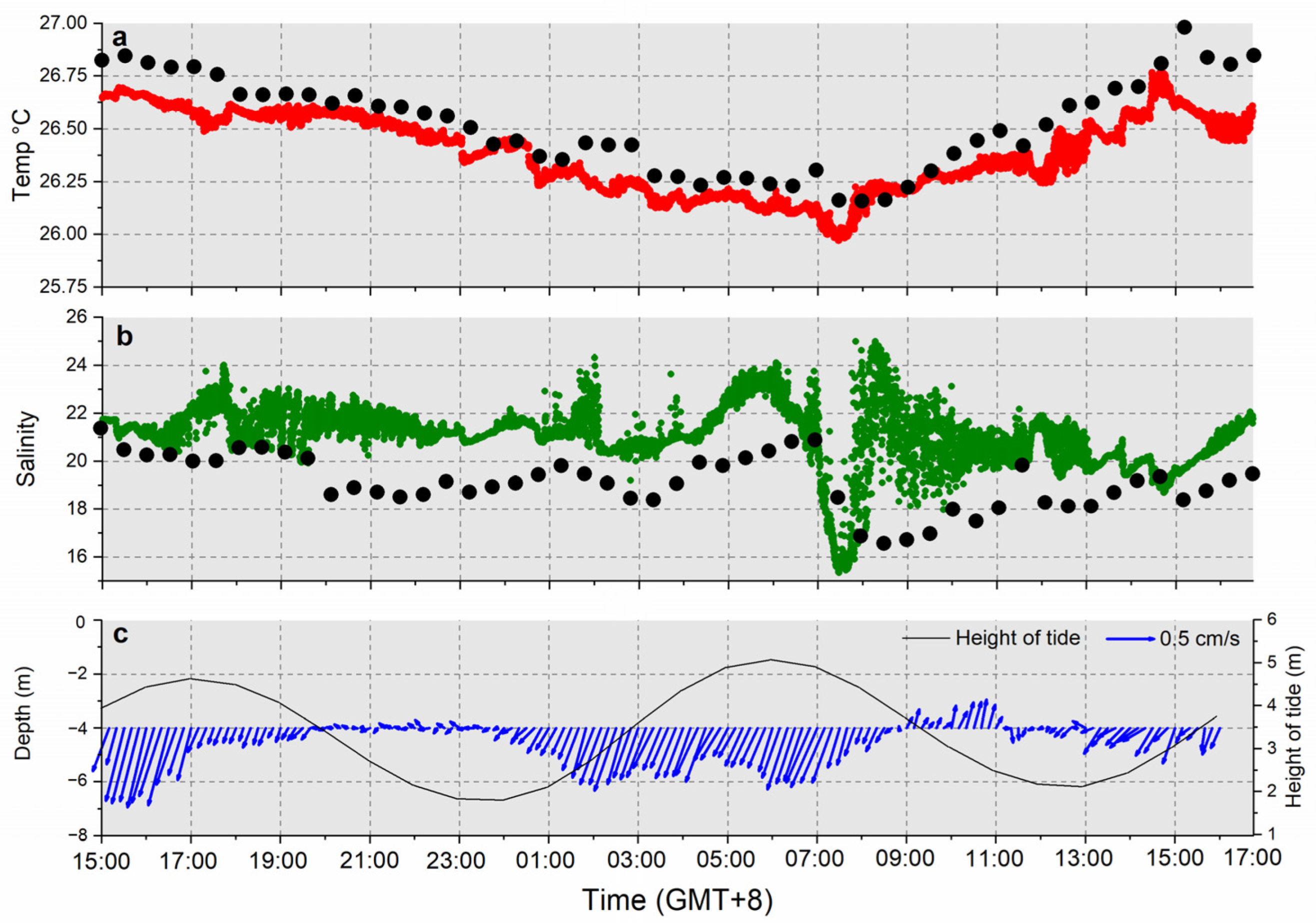
3.1.2. Minjiang Estuary

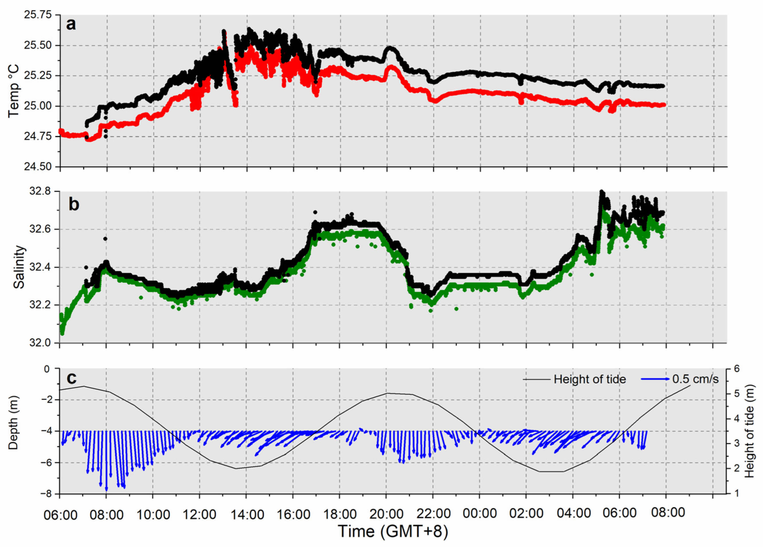
The linear regression of temperature data gathered from the ME and SBE-37 yielded T_Buoy = 2.784 + 1.111T_SBE-37, Pearson’s r = 0.928, and n = 306. The regression of salinity data obtained from the buoy and SBE-37 resulted in SAL_Buoy = 13.641 + 0.259SAL_SBE-37, Pearson’s r = 0.291, and n = 306. It should be noted that salinity data from the buoy showed a significant offset around 3–4 units lower than that of the SBE-37 data (p < 0.05). Near the minimum salinity (approximately 15), the buoy had a small salinity deviation.

The diel temperature variation scenario at the ME differed from that at the DW. The temperature dropped to around 25.9 °C at 7 a.m. and peaked at approximately 26.7 °C at 2 a.m. This suggested that solar radiation was the primary driver of the diel temperature variation, and any effect of the tide on temperature could only be inferred from the lowest temperature after sunrise. During high tide at 6 a.m., warmer offshore water acted as a heat source (Figure 3a).

Buoys located at the ME were dominated by mixohaline water with a salinity ranging between 15 and 25. The salinity exhibited considerable fluctuations due to tidal influence, with a steep variation observed between 6 a.m. and 8 a.m. during the falling tide stage after reaching the high-tide level. Additionally, maximum southward current velocities were recorded. During the two-hour period, salinity initially decreased from approximately 24 to 16 but then returned to around 25 at roughly 8 a.m. due to the weakening of the current velocity (Figure 3b).

The prevailing current direction at the ME was predominantly southwestward, with high current velocities occurring primarily during periods of high tide. By contrast, during periods of low tide, the northward current velocities were measurably lower (Figure 3c).

3.1.3. Huangqi

During the cruise, the HQ was able to conduct regular maintenance on the EXO-2 sensor, resulting in more frequent data acquisition for improved comparison and calibration. The temperature data obtained from the buoy and SBE-37 were analyzed through linear regression, which yielded T_Buoy = 1.730 + 0.937T_SBE-37, Pearson’s r = 0.968, and n = 8636. Similarly, the buoy and SBE-37 were used to obtain salinity data, which resulted in a linear regression of SAL_Buoy = −1.805 + 1.057SAL_SBE-37, Pearson’s r = 0.223, and n = 8636. The salinity data obtained from the buoy exhibited minor divergence, with values up to 0.1 salinity units lower than the SBE-37 data (p < 0.05).

The diel temperature variation measured at the HQ showed a single peak heating–cooling cycle. At 7 a.m., the temperature reached its lowest point of about 24.7 °C, while it peaked at approximately 25.6 °C between 2 p.m. and 3 p.m. Between 1 p.m. and 5 p.m., the temperature fluctuated within a narrow range of 0.6 °C. In other time frames, the temperature trend changes were smooth (Figure 4a).

A consistent diel rhythm was observed between salinity and tide levels at the HQ. As a result, the highest salinity levels were recorded between 5 p.m. and 10 p.m., at approximately 32.6. Additionally, higher salinity water was observed between 5 a.m. and 8 a.m., with a salinity of approximately 32.7. Low salinity was mainly observed during low-tide periods, between 11 a.m. and 2 p.m. and from 10 p.m. to 2 a.m.. The salinity level was approximately 32.3 during these periods, as depicted in Figure 4b.

The flow direction at the buoy station at HQ was predominantly south-bound during high tide levels and southwest-bound at low tide levels. Additionally, the current’s velocities were higher during the receding tide period as compared with the incoming tide (Figure 4c).

According to the T-S properties, the temperature fluctuated no more than 2 °C across three buoy stations, with the highest temperature recorded at the ME by the DW; the lowest temperature was observed at the HQ. Furthermore, the DW had the highest level of salinity, followed by the HQ, and the ME had the lowest. It is noteworthy that the salinity at the ME, situated in the estuarine area, remained below 25, with the lowest recorded value being approximately 15. Overall, concerning potential density, the ME exhibited the lowest value, followed by the HQ. Conversely, the DW demonstrated the highest density (Figure 5).

3.2. Chemical Parameters

3.2.1. Douwei

The pH data obtained from the buoy and EXO-3 were analyzed through linear regression, revealing pH_Buoy = 2.362 + 0.700pH_Exo-3, Pearson’s r = 0.381, and n = 55. It was found that the pH values obtained from EXO-3 were relatively stable, ranging from 8.10 to 8.15, when compared with those acquired by the buoy. However, the variation patterns of the pH data between the buoy and EXO-3 were inconsistent, as depicted in Figure 6a. Furthermore, the analysis of dissolved oxygen (DO) data through linear regression indicated the equation DO_Buoy = 1.168 + 0.882DO_Exo-3, Pearson’s r = 0.911, and n = 55. Although the DO readings from the buoy were 0.1–0.4 mg/L higher than those from EXO-3 (p < 0.05), both sets of data exhibited a synchronous diel variation pattern, as illustrated in Figure 6b. The diel variation in DO showed a bimodal pattern. For example, based on the EXO-3 data, DO remained stable between 6.0 and 6.2 mg/L during the dark period. Subsequently, from 7:00 to 8:00 in the morning, DO began to increase, reaching a maximum concentration of approximately 6.7 mg/L at 12:00. As stated in Section 3.1.1, the impact of tides resulted in a considerable decrease in temperature and salinity from noon to 4 p.m. This caused a fluctuation in the dissolved oxygen levels during the same period. Subsequently, as it reached high tide, the DO reached its second highest value, approximately 6.6 mg/L. Therefore, it can be concluded that the influx of low-salinity and low-temperature water, due to the rising tide, had a discernible impact on the DO levels.

3.2.2. Minjiang Estuary

The pH and dissolved oxygen distribution patterns at the ME closely followed the diel variation in temperature. A linear regression analysis of pH data from the buoy and EXO-3 resulted in pH_Buoy = −1.612 + 1.153pH_Exo-3, Pearson’s r = 0.833, and n = 51. As with the DW, the pH detected by the buoy was lower than that obtained by EXO-3 (p < 0.05), with a difference of approximately 0.2 (Figure 6c). Taking the EXO-3 dataset as an example, the pH ranged from 8.3 to 8.6, with the lowest value occurring in the morning and the highest in the afternoon. The relationship between DO data from the buoy and EXO-3 was modeled using linear regression and resulted in DO_Buoy = −1.485 + 1.219DO_Exo-3, Pearson’s r = 0.899, and n = 51. The DO values obtained by the buoy were in good agreement with those of EXO-3. The DO concentration fluctuated from 7.0 to 10.2 mg/L, with the lowest value recorded in the morning and the highest in the afternoon. The water with lower salinity exhibited lower DO levels. Nevertheless, the DO values were higher compared with the ones recorded at DW (Figure 6d).

3.2.3. Huangqi

A linear regression analysis was conducted on pH data obtained from the buoy and the EXO-3 sensor, resulting in the equation pH_Buoy = −0.643 + 1.057pH_Exo-3, Pearson’s r = 0.937, and n = 8636. The pH measurements captured by the buoy were consistently lower than those obtained by EXO-3 (p < 0.05), with a difference of approximately 0.3 (Figure 6e). Taking the EXO-3 data as an example, the pH varied between 8.1 and 8.3, with a maximum value at 13 p.m., which might be related to the water instability in the period of low tide level. The temperature of the corresponding time periods also fluctuated greatly. The EXO-3- and buoy-derived DO data correlated well, with a linear regression of DO_Buoy = 0.333 + 1.016DO_Exo-3, Pearson’s r = 0.985, and n = 8636 (Figure 6f). The DO values obtained by the buoy were in good agreement with those of EXO-3. The DO values acquired by the buoy matched those of EXO-3. The DO concentration ranged from 5.5 to 8.0 mg/L, with the minimum value recorded between 6 and 12 a.m. and the maximum value recorded in the afternoon. The DO values at low tide levels exhibited significant fluctuations during the morning, displaying a strong correlation with higher flow velocities during periods of high tide.

3.3. Chlorophyll and Phycoerythrin Concentration

3.3.1. Douwei

The buoy-obtained chlorophyll data plotted against the EXO-3 values yielded a linear regression of Chl_Buoy = −0.016 + 0.845Chl_Exo-3, Pearson’s r = 0.542, and n = 55. The concentration of chlorophyll remained between 1.0 and 2.0 μg/L for most of the observation period. However, the highest concentration (more than 4.0 μg/L) predominantly appeared between 10 a.m. and 4 p.m., which correlated with the DO variation, as shown in Figure 7a. During periods of high chlorophyll concentration, similar to the bimodal pattern of dissolved oxygen distribution, the levels of chlorophyll and phycoerythrin fluctuated due to tidal-level variations. A linear regression between phycoerythrin data obtained from the buoy and EXO-3 revealed PE_Buoy = −0.747 + 0.488PE_Exo-3, Pearson’s r = 0.583, and n = 55. The pattern of variation in phycoerythrin was consistent with that of chlorophyll. Throughout most of the experiment, the concentration of phycoerythrin was in the range of 2.0–4.0 μg/L. However, between the hours of 10 a.m. and 4 p.m., the maximum concentration varied between 6.0 and 12.0 μg/L, as illustrated in Figure 7b. The buoy-derived phycoerythrin concentration was comparatively lower than that detected by EXO-3, with a difference of approximately 0.220 μg/L (p < 0.05).

3.3.2. Minjiang Estuary

A linear regression was conducted to compare chlorophyll data gathered from the buoy and EXO-3, resulting in Chl_Buoy = −3.044 + 1.329Chl_Exo-3, Pearson’s r = 0.678, and n = 51. Chlorophyll varied between less than 5.0 μg/L and nearly 70 μg/L, with minimum values observed before sunrise and a maximum value at 4 p.m. (Figure 7c). Similarly, a linear regression was performed for phycoerythrin data obtained from the buoy and EXO-3, yielding PE_Buoy = −12.901 + 1.553PE_Exo-3, Pearson’s r = 0.741, and n = 51. The variation pattern in phycoerythrin was consistent with that of chlorophyll. The concentration of phycoerythrin ranged from 10.0 to 140.0 μg/L, which was nearly two times higher than the concentration of chlorophyll (p < 0.05) (refer to Figure 7d).

3.3.3. Huangqi

The linear regression between chlorophyll data obtained from the buoy and EXO-3 resulted in Chl_Buoy = 0.178 + 0.827Chl_Exo-3, Pearson’s r = 0.876, and n = 8636. The linear regression between phycoerythrin data obtained from the buoy and EXO-3 was PE_Buoy = −2.606 + 0.896PE_Exo-3, Pearson’s r = 0.940, and n = 8636. A comparison between the water quality at DW and ME and that at HQ revealed that chlorophyll and phycoerythrin concentrations were more varied and displayed a multi-peak distribution pattern at the latter. The concentration of chlorophyll ranged from ~2.0 μg/L to almost 25 μg/L, exhibiting four periods of high concentration, specifically 1 p.m. to 2 p.m., followed by 4 p.m. to 5 p.m. and 7 a.m. to 9 a.m., with a minor increase in concentration at midnight (Figure 7e). The phycoerythrin concentration exhibited a variation pattern consistent with that of chlorophyll, ranging from 2.0 to 45 μg/L, which was also approximately twice the concentration of chlorophyll (Figure 7f).

3.3.4. Chlorophyll a and Phycoerythrin Concentration in Water Samples

The chlorophyll a and phycoerythrin concentrations in the water samples at each station were consistent with those obtained using the buoy sensor. The chlorophyll a concentration observed in the water sample at the DW ranged from 1.161 to 5.820 μg/L, as opposed to the range of 1.0 to 20.0 μg/L detected by the buoy sensors. The phycoerythrin concentration obtained from the water sample at the DW ranged from 0.334 to 4.331 μg/L compared with the range of 2.0 to 14.0 μg/L measured by the buoy sensors (Figure 8a). Unlike the scenario at DW, where the concentration of chlorophyll a exceeded that of phycoerythrin, both ME and HQ showed the opposite pattern. Specifically, the water sample taken at the ME had a chlorophyll a concentration range of 2.809 to 8.567 μg/L, while the buoy sensors measured a chlorophyll a concentration range of 5.0 to almost 70.0 μg/L. Again at ME, the phycoerythrin concentration values varied from 3.011 to 18.317 μg/L (Figure 8b). The concentration of chlorophyll a in the water sample collected at the HQ ranged from 1.562 to 6.861 μg/L, which is lower than the range of 2.0 to 25.0 μg/L measured by the buoys (p < 0.05). The phycoerythrin concentration in the same water sample ranged from 2.355 to 12.839 μg/L, while the buoys detected a range of 2.0 to 45.0 μg/L (Figure 8c).

Upon a comparison of the upper and lower limits of chlorophyll a and phycoerythrin concentration at three buoy stations, it was determined that the order of the stations was ME > HQ > DW. Furthermore, the phycoerythrin/chlorophyll a ratio can serve as an index to reflect the composition of the phytoplankton community. At the DW, the phycoerythrin/chlorophyll a ratio varied from 0.215 to 0.995, while at the ME, it ranged from 0.953 to 3.311, and at the HQ, it ranged from 0.830 to 3.446. Phycoerythrin is a light-harvesting pigment that acts as an accessory to chlorophyll a in phytoplankton groups such as Synechococcus, cryptophytes, and dinoflagellates. Higher phycoerythrin/chlorophyll a ratios at ME and HQs were mainly observed in the early morning and in the afternoon when available light was strongest. This is consistent with the characteristics of phycoerythrin as a light-harvesting pigment. In the early morning, the gradually increasing light induced the synthesis of phycoerythrin, thus providing the energy needed for phytoplankton growth. In the afternoon, the rate of phycoerythrin synthesis was faster when the daily maximum light intensity was reached.

4. Discussion

4.1. Phytoplankton Diel Variation in Different Water Masses

The Taiwan Strait serves as a crucial waterway linking the East China Sea and the South China Sea. The complex topography and monsoonal influence of the region lead to intricate water mass and current characteristics [18]. The water masses consist of the South China Sea Warm Current, the Kuroshio Current, the Zhe–Min Coastal Current, and the Taiwan Bank Upwelling Water [4,5]. The South China Sea Warm Current and Kuroshio Current intrude into the Taiwan Strait during June–August, coinciding with the southwestern monsoon period. Interestingly, the prevailing southwestern wind not only induces this intrusion but also causes coastal upwelling [19]. Conversely, during September–March, the Zhe–Min Coastal Current flows southward, with its effects extending to the coastal region of Fujian and the northern South China Sea [18]. Hence, the water mass composition within the Taiwan Strait is intricate, and in summer, the river plume and coastal upwelling also influence the neighboring coastal region.

During the rainy season, the Taiwan Strait is impacted by the discharge of multiple rivers, including the Minjiang River, Jiulongjiang River, Hanjiang River, and even the Pearl River plume extending to the Taiwan Strait [20]. Among these, the Minjiang River has the most significant impact on the water mass and environmental parameters in the Taiwan Strait. The National Water Regime Annual Report 2018 (http://xxzx.mwr.gov.cn/xxgk/gbjb/sqnb/201912/t20191231_1384651.html, accessed on 30 June 2020) notes significant monthly discharge fluctuations in the Minjiang River. The highest discharge level in 2018 was recorded in June. The yearly mean flow of the Minjiang River recorded at the Zhuqi Hydrological Station in 2018, measuring 1010 m³/s, demonstrated a decrease compared with the multi-year climatic mean of 1670 m³/s. This reduction was particularly noticeable during the flood period from May to September, when the discharge dropped to 1270 m³/s, also being lower than the climatic mean of 2450 m³/s. Despite the lower runoff in 2018, the highest value, 5780 m³/s, was reached on June 7th during our research expedition. From Figure 5, it can be inferred that the salinity at the ME ranged between 15 and 25, indicating a mixture of riverine and sea water, which is typical of estuaries. Conversely, the DW and HQ showed typical characteristics of seawater salinity. In particular, the HQ exhibited higher salinity, influenced by coastal upwelling.

The three buoy stations were dominated by different water masses. The ME was mainly influenced by the Minjiang River plume, resulting in high-temperature, low-salinity water. The HQ experienced coastal upwelling, which led to low-temperature, high-salinity water. The DW had mixed water from the Taiwan Strait, leading to high-temperature, high-salinity water. The 24 h cumulative chlorophyll a concentration order for the buoys was ME (10.280 μg/L) > HQ (7.411 μg/L) > DW (4.124 μg/L) (p < 0.05). Although ME had a lower nighttime biomass proportion than DW and HQ (23.9% vs. 30.9% and 29.6%, respectively), its 24 h cumulative biomass was significantly higher (p < 0.05) (Figure 9). Additionally, there was no significant difference in nighttime biomass between the ME (3.825 ± 0.591 μg/L) and HQ (3.277 ± 0.588 μg/L), which both recorded slightly higher amounts of nighttime biomass than the DW (1.159 ± 0.460 μg/L). Although lower values were observed for the water samples compared with the buoy sensor, there were no significant differences between the water sample and sensor data concentration in most instances when the concentration lay between 1.0 and 2.0 μg/L. The discrepancy in data between water samples and the buoy sensor was primarily observed in the frequency band with high value distribution. This was mainly because some of the particulates showing color in the water column (both organic and inorganic particles) could not be distinguished by the buoy sensors, but the phytoplankton fluorescence signals could be determined to a relatively purified extent when measured using the fluorescence method.

The differences in chlorophyll a concentration among the three buoy stations seem to be mainly due to the physiological actions of phytoplankton during daylight hours (Figure 9). The night-to-day ratio of chlorophyll a, approximately 3:7, has been observed in numerous coastal regions, including the Mediterranean Sea [21], the coastal area in the north Atlantic [22], the east coast of the United States [23], and the Yellow Sea/Bohai Sea of China [24]. In the present study, the night-to-day ratio of chlorophyll a at the ME was lower than 3:7. This implies that the biomass of phytoplankton growth during the daytime in the estuary has a greater contribution compared with previous studies. Despite abundant nutrients, phytoplankton growth may be light-limited due to the high turbidity in estuarine water. At the ME, the early morning hours coincided with the high-tide phase, when turbidity was low compared with the low-tide phase, allowing phytoplankton to grow rapidly as light intensity gradually increased, increasing the efficiency of biomass growth during the day and resulting in a higher proportion of cumulative biomass during the day. Nevertheless, the chlorophyll a concentration at the ME was 1.56 and 2.18 times higher than that at HQ and DW, respectively (p < 0.05). Hence, when conducting sampling beyond the established time-series study, assessing the biomass at a research station using the day/night corrections model might require a consideration of the unique characteristics of the water mass, particularly in estuaries and the river-plume-affected regions [23].

For the HQ, despite the lack of prominent upwelling features, the distinct low-temperature, high-salinity water suggested a deep-water influence. Therefore, it was concluded that this area is potentially impacted by coastal upwelling at its periphery. Based on the approximate diurnal biomass ratio at the HQ and DW, even with an increase in nutrients due to upwelling, the change in phytoplankton may not be as significant as in the estuary. This further supports the notion that the biomass of phytoplankton in the estuary is affected by the coupling regulation of nutrients and turbidity. Of course, the tide significantly affects the coastal area regardless of the water masses.

4.2. Tidal Influence

In coastal marine environments, tides are vital to controlling the diurnal variation in phytoplankton biomass. For a 24 h tidal cycle, there are two main effects: tidal current speeds (about 6 h) and horizontal water motion (about 12 h) [25]. In the previous study, the tidal cycle could explain up to 50% of the chlorophyll a variation [26]. In tropical estuaries, tidal action impacts the mixing of riverine end elements and offshore seawater end elements. This caused an increase in the complexity of nutrients, turbidity, and dissolved oxygen levels in the estuary, resulting in a significant shift in the phytoplankton biomass [27,28]. In addition to the role of the tide in the estuary, the upwelling system could result in changes to the phytoplankton biomass caused by the coupling of the internal tides and upwelling [29]. Semi-diurnal tides are predominant in most areas of the Taiwan Strait. In the present study, it was observed that the tide levels at all three stations were high at dawn and in the early morning, while low tide levels occurred at midnight and noon. It is evident that all three stations exhibited a notable decline in chlorophyll a concentration during the high-to-low tide levels from dawn to midnight. The impact of the declining and subsequently escalating tide levels on the concentration of chlorophyll a in the heliography resulted in three distinct patterns at the three stations, as the maximum tide level was seen during early morning (Figure 10).

Pattern 1: Light trumps tidal influences, represented by the DW (Figure 10a). Despite the influence of tides on the concentration of chlorophyll a, its peak value occurred during the strongest light at noon. Therefore, light intensity had a greater effect than tides. This pattern was closely connected to the composition of the water mass in which the DW is situated. As tidal shifts only minimally affect the characteristics of water masses, their effect is not particularly strong. In other words, the water mass characteristics in the vicinity remain stable, resulting in corresponding stability in the phytoplankton biomass.

Pattern 2: Low-tide, high-biomass, represented by the ME (Figure 10b). Chlorophyll a concentrations were not high in the early morning at the ME. However, as the tide receded, they peaked at noon during the lowest tide level. Subsequently, during the next high tide in the afternoon, chlorophyll a concentrations remained elevated. The chlorophyll a concentration in estuaries reflects diurnal variation influenced by tides [27,28]. During the early morning to midday, as the tide level decreased, the meta-input at the estuarine end increased its dominance and more nutrients became available for phytoplankton. This coincided with gradually increasing light conditions that can stimulate rapid phytoplankton growth. In the late afternoon, at high tide levels, the river end gradually receded in dominance and turbidity concurrently decreased. This resulted in improved light conditions and consequently the maintenance of high levels of chlorophyll a.

Pattern 3: High-tide, high-biomass, represented by the HQ (Figure 10c). At the HQ, the highest concentration of chlorophyll a was observed during the morning, when the highest tide occurred. Subsequently, the concentration decreased gradually as the tide level lowered. Interestingly, a high concentration of chlorophyll a occurred in the afternoon after the tide level hit its minimum point. Although it is uncommon for chlorophyll a concentration to be high in the early morning, this may occur in upwelling-affected areas [25]. This could indicate a vertical diurnal movement of phytoplankton [21], or it could result from the combination of upwelling and high tide, which brings high levels of biomass from the subsurface to the surface [29]. It is reasonable to assume that the water column at the HQ is affected by coastal upwelling, which explains this trend. The elevated chlorophyll a concentration during the late afternoon could primarily result from the buildup of biomass produced by indigenous phytoplankton growth.

In summary, the impact of tides on phytoplankton biomass is a highly intricate and dynamic process. An unbiased analysis of tide effects is essential, considering the characteristics of the water mass and its interaction with vital phytoplankton modulators such as light and nutrients. High-temporal-resolution observations are also crucial in comprehending the complex dynamics of phytoplankton biomass. At the same time, this is coupled with seasonal variations in phytoplankton biomass; this may be the result of the response of the phytoplankton itself to characteristics of seasonal elements such as temperature and solar radiation, or it may be due to the influence of the inter-seasonal hydrodynamic context (e.g., river runoff, wind stress, and vertical mixing).

5. Conclusions

Marine environmental monitoring in coastal areas is essential for obtaining high-resolution data. The time-series monitoring of water quality using buoys can effectively be used to predict the occurrence of ecological disasters such as algal blooms and hypoxia. The marine environment on the west side of the Taiwan Strait is significantly impacted by human activities, due to its high population. Moreover, the hydrodynamics of the water column in the strait are intricate and dynamic, leading to significant transformations in environmental factors, particularly in biological parameters. The present study may serve as a point of reference for related research, and the major conclusions are outlined below:

• There were significant differences in the characteristics of the water masses at the three buoy stations. The Minjiang Estuary Station was mainly influenced by the river plume, while the Huangqi Station was mainly influenced by coastal upwelling. The Douwei Station exhibited typical Taiwan Strait warm-water characteristics. The corresponding phytoplankton chlorophyll a concentration was highest at the Minjiang Estuary, followed by Huangqi, and was the lowest at Douwei.
• The diurnal variation in phytoplankton was jointly regulated by water masses, tides, and light. At the three stations, three different response patterns were observed. The station at Minjiang Estuary, with the highest biomass, was notably influenced by tidal action. On the other hand, the Huangqi Station, being affected by upwelling, exhibited two peaks in chlorophyll a concentration, which were attributed to tides and light, respectively. In contrast, the lowest concentration of phytoplankton chlorophyll a was found at Douwei Station, which was mainly attributed to the stable water mass found here compared with ME and HQ, which was not affected by physical processes.

References

1. Falkowski, P.G.; Barber, R.T.; Smetacek, V. Biogeochemical Controls and Feedbacks on Ocean Primary Production. Science 1998, 281, 200–206. [Google Scholar] [CrossRef] [PubMed]
2. Manizza, M.; Quéré, C.L.; Watson, A.J.; Buitenhuis, E.T. Bio-optical feedbacks among phytoplankton, upper ocean physics and sea-ice in a global model. Geophys. Res. Lett. 2005, 32, L05603. [Google Scholar] [CrossRef]
3. Smayda, T.J.; Reynolds, C.S. Community Assembly in Marine Phytoplankton: Application of Recent Models to Harmful Dinoflagellate Blooms. J. Plankton Res. 2001, 23, 447–461. [Google Scholar] [CrossRef]
4. Jan, S.; Sheu, D.D.; Kuo, H.-M. Water mass and throughflow transport variability in the Taiwan Strait. J. Geophys. Res. Ocean. 2006, 111, C12012. [Google Scholar] [CrossRef]
5. Jan, S.; Wang, J.; Chern, C.-S.; Chao, S.-Y. Seasonal variation of the circulation in the Taiwan Strait. J. Mar. Syst. 2022, 35, 249–268. [Google Scholar] [CrossRef]
6. Hsu, P.-C.; Lu, C.-Y.; Hsu, T.-W.; Ho, C.-R. Diurnal to Seasonal Variations in Ocean Chlorophyll and Ocean Currents in the North of Taiwan Observed by Geostationary Ocean Color Imager and Coastal Radar. Remote Sens. 2020, 12, 2853. [Google Scholar] [CrossRef]
7. Gattuso, J.P.; Frankignoulle, M.; Wollast, R. Carbon and Carbonate Metabolism in Coastal Aquatic Ecosystems. Annu. Rev. Econ. 1998, 29, 405–434. [Google Scholar] [CrossRef]
8. Simpson, J.H.; Brown, J.; Matthews, J.; Allen, G. Tidal straining, density currents, and stirring in the control of estuarine stratification. Estuaries 1990, 13, 125–132. [Google Scholar] [CrossRef]
9. Thyssen, M.; Mathieu, D.; Garcia, N.; Denis, M. Short-term variation of phytoplankton assemblages in Mediterranean coastal waters recorded with an automated submerged flow cytometer. J. Plankton Res. 2008, 30, 1027–1040. [Google Scholar] [CrossRef]
10. Tseng, H.-C.; You, W.-L.; Huang, W.; Chung, C.-C.; Tsai, A.-Y.; Chen, T.-Y.; Lan, K.-W.; Gong, G.-C. Seasonal Variations of Marine Environment and Primary Production in the Taiwan Strait. Front. Mar. Sci. 2020, 7, 38. [Google Scholar] [CrossRef]
11. Zhong, Y.; Liu, X.; Xiao, W.; Laws, E.A.; Chen, J.; Wang, L.; Liu, S.; Zhang, F.; Huang, B. Phytoplankton community patterns in the Taiwan Strait match the characteristics of their realized niches. Prog. Oceanogr. 2020, 186, 102366. [Google Scholar] [CrossRef]
12. Zhong, Y.; Hu, J.; Laws, E.A.; Liu, X.; Chen, J.; Huang, B. Plankton community responses to pulsed upwelling events in the southern Taiwan Strait. ICES J. Mar. Sci. 2019, 76, 2374–2388. [Google Scholar] [CrossRef]
13. Wang, Y.; Kang, J.-H.; Ye, Y.-Y.; Lin, G.-M.; Yang, Q.-L.; Lin, M. Phytoplankton community and environmental correlates in a coastal upwelling zone along western Taiwan Strait. J. Mar. Syst. 2016, 154, 252–263. [Google Scholar] [CrossRef]
14. Shang, S.L.; Zhang, C.Y.; Hong, H.S.; Shang, S.P.; Chai, F. Short-term variability of chlorophyll associated with upwelling events in the Taiwan Strait during the southwest monsoon of 1998. Deep. Sea Res. Part II Top. Stud. Oceanogr. 2004, 51, 1113–1127. [Google Scholar] [CrossRef]
15. Zhang, Y.; Su, J.-Z.; Su, Y.-P.; Lin, H.; Xu, Y.-C.; Barathan, B.P.; Zheng, W.-N.; Schulz, K.G. Spatial Distribution of Phytoplankton Community Composition and Their Correlations with Environmental Drivers in Taiwan Strait of Southeast China. Diversity 2020, 12, 433. [Google Scholar] [CrossRef]
16. Parsons, T.; Maita, Y.; Lalli, C.M. Amanual of chemical and biological methods for seawater analysis. In Biological Oceanographic Processes; Parsons, T., Ed.; Pergamon Press: New York, NY, USA, 1984; p. 173. [Google Scholar]
17. Kasinak, J.-M.E.; Holt, B.M.; Chislock, M.F.; Wilson, A.E. Benchtop fluorometry of phycocyanin as a rapid approach for estimating cyanobacterial biovolume. J. Plankton Res. 2015, 37, 248–257. [Google Scholar] [CrossRef]
18. Hong, H.; Chai, F.; Zhang, C.; Huang, B.; Jiang, Y.; Hu, J. An overview of physical and biogeochemical processes and ecosystem dynamics in the Taiwan Strait. Cont. Shelf Res. 2011, 31, S3–S12. [Google Scholar] [CrossRef]
19. Tang, D.; Kester, D.R.; Ni, I.-H.; Kawamura, H.; Hong, H. Upwelling in the Taiwan Strait during the summer monsoon detected by satellite and shipboard measurements. Remote Sens. Environ. 2002, 83, 457–471. [Google Scholar] [CrossRef]
20. Chen, Z.; Pan, J.; Jiang, Y.; Lin, H. Far-reaching transport of Pearl River plume water by upwelling jet in the northeastern South China Sea. J. Mar. Syst. 2017, 173, 60–69. [Google Scholar] [CrossRef]
21. Brunet, C.; Casotti, R.; Vantrepotte, V. Phytoplankton diel and vertical variability in photobiological responses at a coastal station in the Mediterranean Sea. J. Plankton Res. 2008, 30, 645–654. [Google Scholar] [CrossRef]
22. O’Boyle, S.; Silke, J. A review of phytoplankton ecology in estuarine and coastal waters around Ireland. J. Plankton Res. 2010, 32, 99–118. [Google Scholar] [CrossRef]
23. Carberry, L.; Roesler, C.; Drapeau, S. Correcting in situ chlorophyll fluorescence time-series observations for nonphotochemical quenching and tidal variability reveals nonconservative phytoplankton variability in coastal waters. Limnol. Oceanogr. Methods 2019, 17, 462–473. [Google Scholar] [CrossRef] [PubMed]
24. Salisbury, J.E.; Jönsson, B.F.; Mannino, A.; Kim, W.; Goes, J.I.; Choi, J.-Y.; Concha, J.A. Assessing Net Growth of Phytoplankton Biomass on Hourly to Annual Time Scales Using the Geostationary Ocean Color Instrument. Geophys. Res. Lett. 2021, 48, e2021GL095528. [Google Scholar] [CrossRef]
25. Blauw, A.N.; Benincà, E.; Laane, R.W.P.M.; Greenwood, N.; Huisman, J. Dancing with the Tides: Fluctuations of Coastal Phytoplankton Orchestrated by Different Oscillatory Modes of the Tidal Cycle. PLoS ONE 2012, 7, e49319. [Google Scholar] [CrossRef] [PubMed]
26. Cereja, R.; Brotas, V.; Cruz, J.P.C.; Rodrigues, M.; Brito, A.C. Tidal and Physicochemical Effects on Phytoplankton Community Variability at Tagus Estuary (Portugal). Front. Mar. Sci. 2021, 8, 675699. [Google Scholar] [CrossRef]
27. Baliarsingh, S.K.; Lotliker, A.A.; Srichandan, S.; Roy, R.; Sahu, B.K.; Samanta, A.; Nair, T.M.B.; Acharyya, T.; Parida, C.; Singh, S.; et al. Evaluation of hydro-biological parameters in response to semi-diurnal tides in a tropical estuary. Ecohydrol. Hydrobiol. 2021, 21, 700–717. [Google Scholar] [CrossRef]
28. Sin, Y.; Jeong, B.; Park, C. Semidiurnal Dynamics of Phytoplankton Size Structure and Taxonomic Composition in a Macrotidal Temperate Estuary. Estuaries Coasts 2015, 38, 546–557. [Google Scholar] [CrossRef]
29. Shanks, A.L.; Morgan, S.G.; Macmahan, J.; Reniers, A.; Jarvis, M.; Brown, J.; Fujimura, A.; Griesemer, C. Onshore transport of plankton by internal tides and upwelling-relaxation events. Mar. Ecol. Prog. Ser. 2014, 502, 39–51. [Google Scholar] [CrossRef]
Figure 1. (a) Map of the study area and buoy stations. (b) Douwei (DW), (c) Minjiang Estuary (ME), and (d) Huangqi (HQ).
Jmse 11 02252 g001
Figure 2. The time series of temperature, salinity, and currents of the surface water at Douwei Buoy Station. (a) Temperature, (b) salinity, and (c) surface currents and height of tide. The black dots denote the buoy data and colored dots denote the SeaBird SBE-37 data within figures (a,b). The black line denotes the tide and blue arrows denote the calibration currents in Figure c.
Jmse 11 02252 g002
Figure 3. The time series of temperature, salinity, and currents of the surface water at Minjiang Estuary Buoy Station. (a) Temperature, (b) salinity, and (c) surface currents and height of tide. The black dots denote the buoy data and colored dots denote the SeaBird SBE-37 data within figures (a,b). The black line denotes the tide and blue arrows denote the calibration currents in Figure (c).
Jmse 11 02252 g003
Figure 4. The time series of temperature, salinity, and currents of the surface water at Huangqi Buoy Station. (a) Temperature, (b) salinity, (c) surface currents and height of tide. The black dots denote the buoy data and colored dots denote the SeaBird SBE-37 data within figures (a,b). The black line denotes the tide and blue arrows denote the calibration currents in (c).
Jmse 11 02252 g004
Figure 5. The T-S properties at three buoy stations. The black triangles denote high tide and inverted triangles denote low tide.
Jmse 11 02252 g005
Figure 6. The time series of pH and DO of the surface water at three buoy stations: (a,b) Douwei, (c,d) Minjiang Estuary, and (e,f) Huangqi. The black dots denote the buoy data, the pink and the blue dots denote pH and DO data for EXO-3. The inverted triangles and triangles denote the lowest and highest tide, respectively.
Jmse 11 02252 g006
Figure 7. The time series of chlorophyll and phycoerythrin of the surface water at three Buoy stations: (a,b) Douwei, (c,d) Minjiang Estuary, and (e,f) Huangqi. The black dots denote the buoy data, and orange and purple dots denote chlorophyll and phycoerythrin data of EXO-3. The inverted triangles and triangles denoted the lowest and highest tide, respectively.
Jmse 11 02252 g007
Figure 8. The time series of Turner chlorophyll a and phycoerythrin of the surface water at three buoy stations: (a) Douwei, (b) Minjiang Estuary, and (c) Huangqi. The orange and purple dots denote chlorophyll a and phycoerythrin, respectively. The inverted triangles and triangles denote the lowest and highest tide, respectively.
Jmse 11 02252 g008
Figure 9. Proportion (pie chart, %) and Turner chlorophyll a concentration (column chart, μg/L) in different water masses at three buoy stations. The proportion indicates the percentage of night (yellow) and daytime (blue) biomass compared with the 24 h accumulation chlorophyll a biomass. The coordinate axis is symbolized as T-S properties.
Jmse 11 02252 g009
Figure 10. Heatmaps of the chlorophyll a (μg/L) on the time–tide matrix at three buoy stations: (a) indicates Douwei, (b) indicates Minjiang Estuary, and (c) indicates Huangqi. The shadow indicates the nighttime and the gray lines indicate the tide level.
Jmse 11 02252 g010