Article

Investigation on the Erosion Characteristics of Liquid–Solid Two-Phase Flow in Tee Pipes Based on CFD-DEM

1
Research Center of Fluid Machinery Engineering and Technology, Jiangsu University, Zhenjiang 212013, China
2
Key Laboratory of Fluid Machinery and Engineering, Xihua University, Chengdu 610039, China
3
Chongqing Pump Industry Co., Ltd., Chongqing 400033, China
4
Fluid Machinery of Wenling Research Institute, Jiangsu University, Wenling 318000, China
*
Authors to whom correspondence should be addressed.
J. Mar. Sci. Eng. 2023, 11(12), 2231; https://doi.org/10.3390/jmse11122231
Submission received: 22 September 2023 / Revised: 11 November 2023 / Accepted: 12 November 2023 / Published: 25 November 2023
(This article belongs to the Special Issue CFD Analysis in Ocean Engineering)

Abstract

:
Tee pipes are widely utilized in pipeline transportation, especially in subsea production systems and the chemical industry. The purpose of this research is to study the influences of gravity direction, conveying parameters and particle properties on the erosion distribution in tee junctions. Investigation using the CFD-DEM coupled method is conducted on the flow mechanisms and erosion characteristics in a tee junction under different flow conditions. Firstly, numerical calculations of liquid–solid two-phase flow in a vertical cylindrical pipe are performed, and the comparison between simulation results and experimental results is carried out. Then, the verified lift and erosion models are used for the numerical calculations of tee pipes. Flow mechanisms and erosion characteristics are numerically investigated through analysis of the velocity profiles, streamlines, and erosion contours. The results indicate that the gravity direction has a nonnegligible influence on the cross-sectional velocity profiles, particularly under the condition of high velocity and high particle concentration. The region with the maximum erosion rate occurred at the branch pipes, about three fourths of the pipe diameter away from the tee junction.

1. Introduction

Pipeline transportation has a series of advantages such as simple structure, large transportation volume, high efficiency, and energy saving, so pipeline transportation is widely used as the most important fluid medium transportation in subsea production systems and the chemical industry. Erosion caused by solid particles is a common problem that endangers the safety of production in the process of pipeline usage, which may cause the device to malfunction or even fail. As common pipeline transportation components, elbows and tees are extensively applied to change the flow direction and guide the fluid medium to divert or combine. However, due to some coarse particles that are inevitably carried in the fluid medium, they continue to wash away the inner wall of the location where the flow direction changes, causing erosion and failure of the pipeline, especially the elbows and tees, resulting in leakage accidents and economic losses. Therefore, it is necessary to reveal the characteristics and mechanism of the erosion process caused by solid particles in the pipeline for accurately predicting the erosion distribution of the pipe inner wall.
Based on the previous literature, many experiments and analytical and numerical research have been carried out to study the erosion mechanisms and characteristics in pipelines. Finnie [1,2] was the first to discuss the removal mechanism of brittle and ductile materials and propose the theory of micro-cutting corrosion–erosion. Bitter [3,4] established a related erosion model based on a modification to Finnie’s model and proposed that the removal of wall material is mainly due to repeated deformation and particle cutting during the particle–wall collision process. Archard [5] and Oka et al. [6,7] established relevant erosion models according to specific experimental conditions. Such models can predict pipeline erosion in industrial applications in some specific engineering environments. The Erosion/Corrosion Research Center (E/CRC) of the University of Tulsa carried out a comprehensive study of 90° elbows and plugged tees regarding the relative erosion rate when carrying dilute particulate flows [8,9].
Wang K et al. [10] conducted a numerical analysis for liquid–solid two-phase flows using the two-way coupled Eulerian–Lagrangian model to predict the erosion in elbows. The results proved the coupling influences between fluid and particles as well as their impact on the elbow erosion. The correlation between the erosion modes and particle Stokes number was also established in their research. Huang Y et al. [11] simulated the erosion of a plugged tee pipe through rock cuttings of the same size and different sizes, and the calculation results indicated that the motion patterns of rock cuttings and the erosion region of the plugged tee change significantly with the growth in particle size. Zamani M et al. [12] found that particle rotation considerably affects particle motion trajectory and consequently the elbow erosion mode due to the increased collision against the elbow wall through a two-way coupled Eulerian–Lagrangian method and strengthened wall treatment. Chen X et al. [13] conducted research on the relative erosion extent between elbows and plugged tee pipes for gas–solid two-phase flow under the condition of atmospheric pressure. The predicted erosion model was utilized to estimate the relative erosion extent and the experiments were performed to prove the precision of the calculation results acquired for gas–sand two-phase flows. Farokhipour A et al. [14] carried out numerical simulations on particle-laden flows under the conditions of various fluid velocities and used a CFD-DEM coupled model to investigate the effects of particle mass loadings in the corresponding geometries. The calculation results show that a plugged tee pipe has greater effectiveness than the elbow as the particle mass loading increases. Liu C et al. [15] performed research on the erosion severity of a 90° elbow through numerical calculation and proposed several factors that affect elbow erosion, including particle velocity, concentration, and impact angle. Yao J L et al. [16] carried out research on elbow erosion through an exhaust pipe with same-sized rock cuttings and found that the range of 45°~60° is the maximum erosion position. Duarte et al. [17] conducted a numerical investigation on the influence of particle mass fraction regarding elbow erosion and found that particle collisions have a nonnegligible effect on the penetration rate (the ratio of wall eroded mass to solid particle mass) even at low and moderate particle mass concentrations. They also found a phenomenon called the cushioning effect, wherein the penetration rate decreases as the particle mass fraction increases.
For obtaining an accurate prediction on the erosion caused by fracturing slurry flow in tee junctions, Zhang J X et al. [18] defined the failure pattern and failure mechanism of tee junctions using macro-properties and scanning electron microscope (SEM) images, which seems to be quite different from what is considered conventional. Charron Y and Whalley P B [19] investigated annular gas–liquid flow in a vertical tee pipe with a horizontal outlet and examined the flow separation mechanisms of different annular flow types. A comparison between flow separation model predictions and existing data is conducted and the effectiveness of several hypotheses provided in mechanical models is examined based on the observations offered from this experiment. Brown G J [20] developed a CFD model to investigate the movement of lye–bauxite pellet liquid–solid two-phase flow in a tee pipe using the Eulerian–Eulerian method combined with the k-ε turbulence model simultaneously; the results verified the validity of the CFD approach for solving erosion failure problems in industry. Zhang J et al. [21] experimentally studied the main factors that affect high-pressure pipeline and tee pipe erosion rates using an advanced erosion and wear testing machine. They also established an erosion rate model based on relevant erosion theories and the erosion experiment results. The results indicated that downstream triplet and dorsal components close to the branch are prone to failure. Costa N P et al. [22] investigated the edge impacts on the internal flow properties as well as the pressure drop through a 90° tee junction with rounded and sharp corners. The results show that the energy losses decrease approximately 10% to 20% in round corners, while the straight flow almost remained the same. Jin H U et al. [23] investigated the wear and erosion properties of gas–solid multiphase flow in a tee pipe through several calculations of inlet pipes with different diameters, and the results indicate that the intersection erosion rate increases when the inlet diameter decreases. Zhang J et al. [24] studied the erosion mechanism of liquid–solid multiphase flow in the manifold tee pipe and predicted the inner wall erosion distribution under four different combination types.
Although numerous studies have been conducted on erosion characteristics in elbows and plugged tees, few efforts have been made to predict the erosion distribution in tee junctions since the flow patterns in the tee pipe are more complex. Furthermore, questions in regard to the optimal use of tee junctions rather than elbows or plugged tees under several working conditions have not yet been adequately solved. The influences of turbulence, particle rebound, and corresponding erosion rates on particle-laden flow through tee junctions are not fully understood. Therefore, it is important to thoroughly understand the impact of these different flow parameters on the stability of the tee junction, that not only can accurately forecast erosion and wear distribution but also can determine appropriate monitoring and investigation measures to keep the pipelines safe under various flow conditions. In this study, a CFD-DEM coupled approach is employed to investigate the flow mechanisms and erosion characteristics in tee junctions under different directions of gravity and conveying parameters (concentration, velocity, particle diameter). It can provide an effective analysis approach to understand the flow mechanisms and can be used to estimate the erosion characteristics in tee junctions.

2. Numerical Model

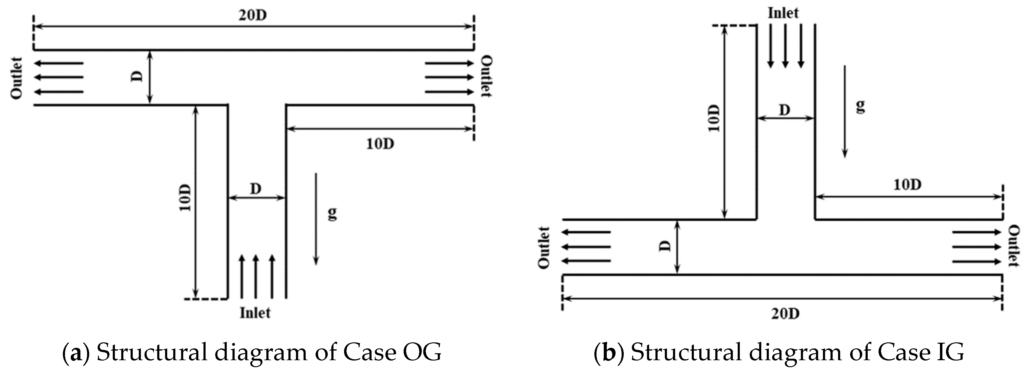
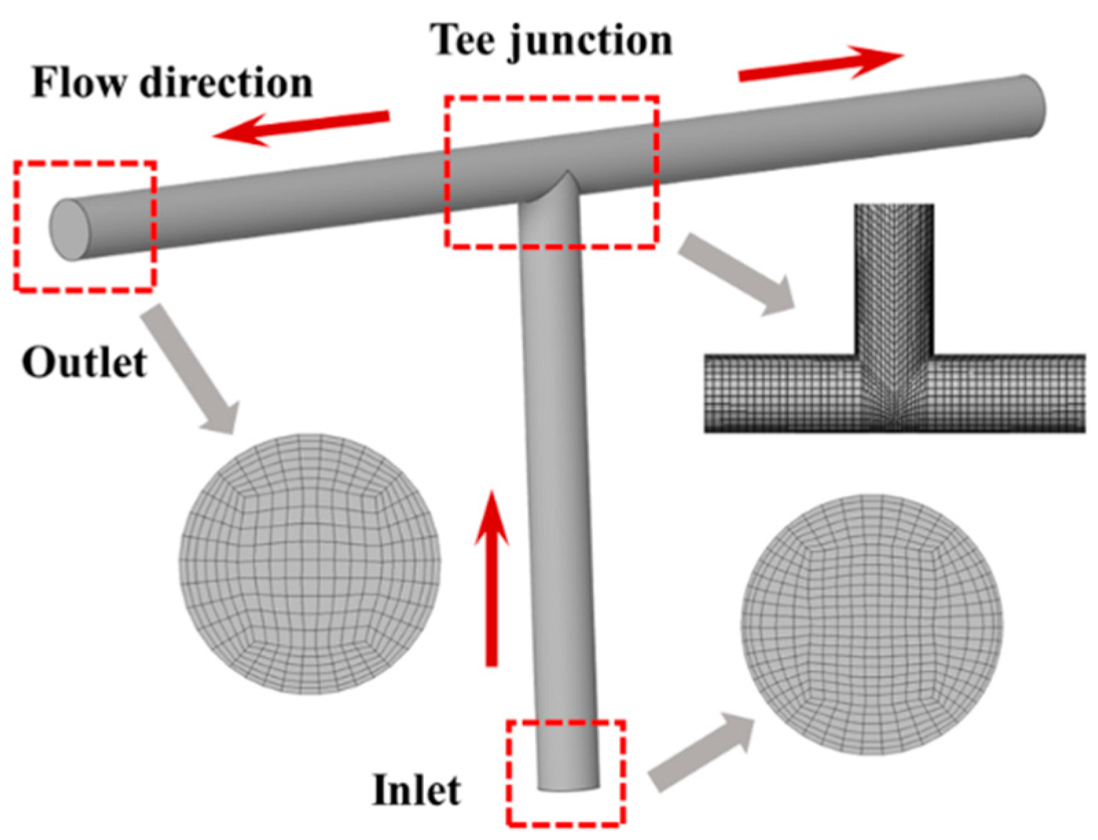
2.1. Tee Pipe Physical Model Establishment

Figure 1 shows the arrangement of tee pipes in two directions of gravity. The direction of gravity in Figure 1a is opposite to the inlet velocity, while that in Figure 1b is identical to the inlet velocity. Both tee pipes are symmetrical and contain two outlets. To facilitate the analysis, all calculation cases for the tee pipes in this study are named with the direction of gravity (i.e., OG and IG represent the inlet velocity opposite to gravity and identical to gravity, respectively), the particle concentration (i.e., 0.5C to 7C, respectively, represent particle concentration = 0.5% to 7%), the inlet velocity (i.e., 3V to 6V, respectively, represent inlet velocity = 3 m/s to 6 m/s), and the particle diameter (i.e., 0.6D to 1.5D, respectively, represent particle diameter = 0.6 mm to 1.5 mm). Thus, Case OG-3V-0.5C-1D represents the numerical calculation of the tee pipe with the inlet velocity of 3 m/s, the particle concentration of 0.5%, and the particle diameter of 1 mm under the flow condition that the inlet velocity direction is opposite to the gravity.
In this study, the established fully coupled CFD-DEM mathematical model and erosion model are utilized to calculate the selected tee pipe. In the following subsections, the parameters, boundary conditions, and grid scheme used in the simulation will be introduced in detail. For better understanding of the flow characteristics when the fluid and particles pass through the tee junction and move downstream through the branch pipes, the numerical simulation of the tee pipe transporting clean water was carried out and analyzed.

2.2. Mathematical Equations

2.2.1. Governing Equations of Liquid Phase

Since the conveying medium in this paper consists of particles and clean water, the fluid is incompressible and the density is constant, which does not vary in three-dimensional space–time. Therefore, the simplified continuity and momentum equations can be expressed as follows (in order to better understand the meaning of each variable in the formula, we distinguish scalars and vectors and make the vectors bold):
t α f ρ f + α f ρ f v f = 0
t α f ρ f v f + α f ρ f v f v f = α f p + α f μ f + μ t v f + v f T + α f ρ f g + F p f
F p f = 1 V i = 1 m F f p  
where ρ f denotes fluid density, v f refers to average fluid velocity, p is pressure, μ f and μ t , respectively, represent the fluid dynamic viscosity and turbulent viscosity, g is the gravity acceleration and the current value is 9.81 m/s2, F p f represents the volume force exerted by particles on the fluid within the fluid grid, F f p represents the total fluid force acting on the particle within the fluid grid, m is the amount of particles in the calculation unit, V is the calculation unit volume, and α f is the volume fraction of the fluid.

2.2.2. Governing Equations of Solid Phase

In the study of solid–liquid two-phase flow, the force on particles affects their motion state, thereby affecting the erosion pattern of components. In this paper, the Euler–Lagrangian approach is adopted, and the particle is considered as a discrete phase, which is solved in EDEM. The particle’s motion follows Newton’s second law and can be expressed by the following equation:
m p d v p d t = F d r a g + F b + F L o t h + F p + F v m + F c
I p d Ω p d t = T c + T f
where F d r a g represents the drag force, F b represents the resultant force of buoyancy and gravity, F L o t h represents the Loth lift force, F p represents the pressure gradient force, F v m represents the virtual mass force, F c represents the contact force between particle and inner wall, Ω p represents the particle angular velocity, I p represents the particle inertia moment, T c and T f , respectively, represent the contact torque and fluid torque, d v p d t represents the particle average acceleration, and m p represents the particle mass.

2.2.3. The Program Interaction and Calculation Algorithm

The modeling of the particle phase by DEM is carried out at the single-particle scale, while the modeling of the fluid phase by CFD is carried out at the computational grid scale. The fluid control equation is solved based on the finite volume method, and the particle motion equation is solved based on the DEM method. The calculation of volume fraction, data transfer between phases, calculation of particle forces and source terms, etc. is implemented in self-developed interface code. The total coupling forces experienced by all particles in the fluid mesh are summed and the summed force is added as a source term to the fluid momentum equation. In addition, particle–turbulence interactions are also considered in the coupling interface. At the beginning of each time step, the coupling interface extracts the information of each particle in the flow field (such as particle position coordinates, volume and particle velocity, etc.) and calculates the particle volume fraction and source term within each CFD grid. Then, the fluid field is solved in ANSYS FLUENT, the obtained fluid information (grid information, fluid velocity and pressure, etc.) is transferred into EDEM, and the fluid force and torque experienced are calculated by each particle to determine the individual particle motion at the next time step.

2.3. Erosion Model

The erosion model proposed by the Erosion/Corrosion Research Center of the University of Tulsa is used in this paper. E/CRC erosion model fully considers the effects of particle shape, impact angle, and collision velocity, which can be written as:
E R = C ( B H ) 0.59 F s v p n F ( α )
F α = 5.3983 α 10.1068 α 2 + 10.9327 α 3 6.3283 α 4 + 1.4234 α 5
where E R represents the erosion rate (kg/kg, indicates the ratio of the mass removed from the wall to the mass of the particle hitting the wall), B H represents the Brinell hardness of wall material, F s represents particle shape factor, v p represents particle impact velocity, C = 2.17 × 10⁻⁷, n = 2.41, and α is the particle impact angle.

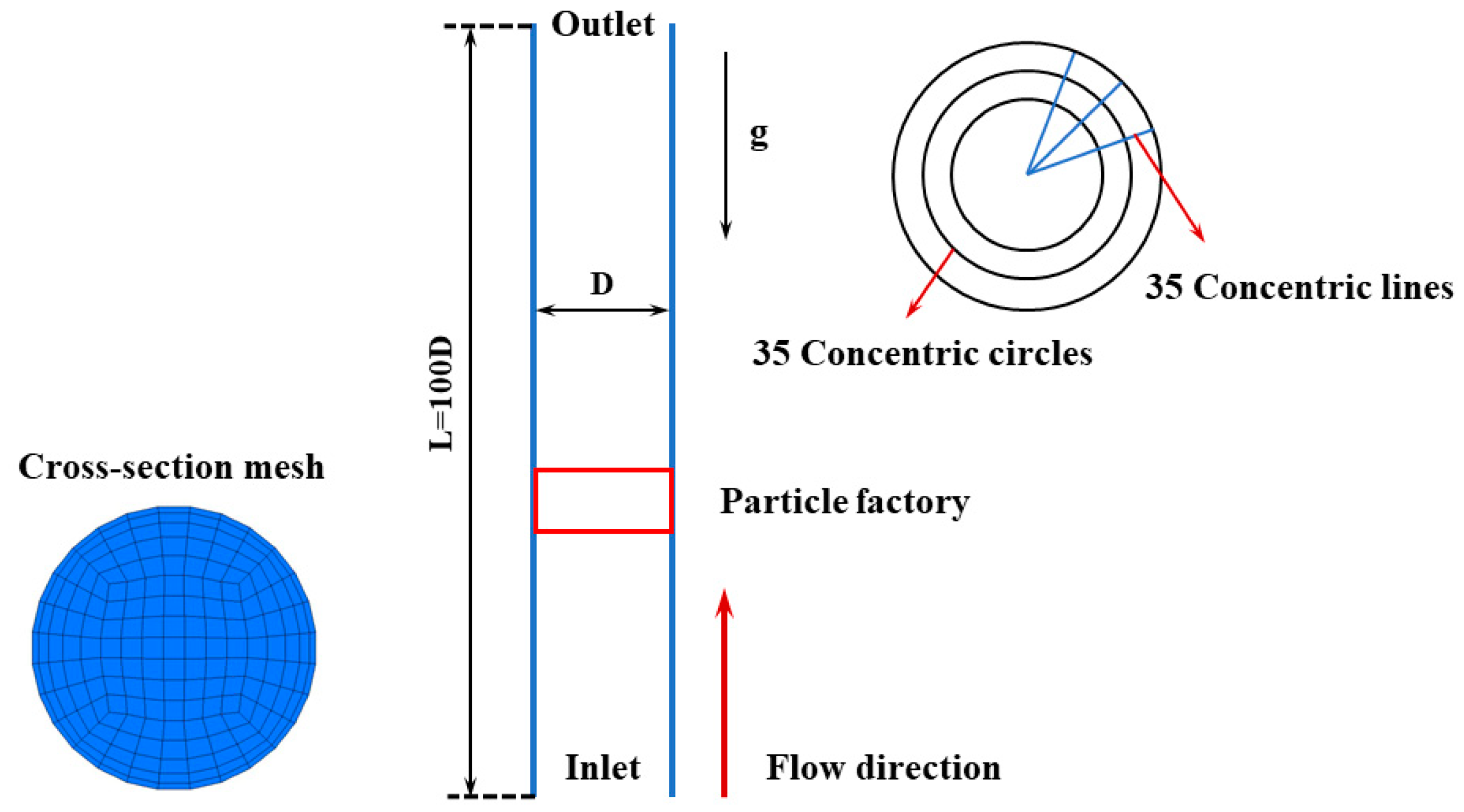
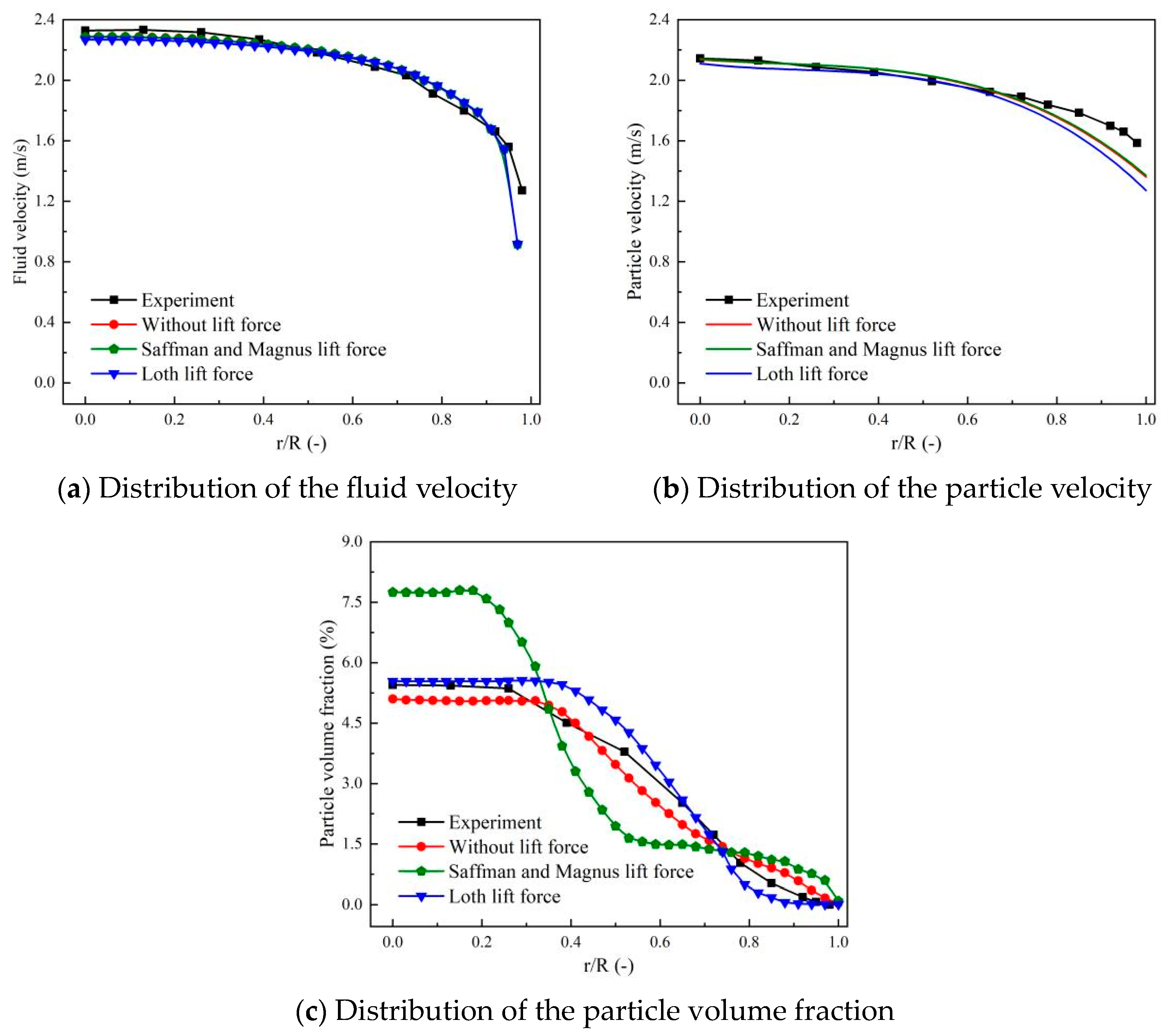
2.4. Numerical Simulation Verification of Vertical Pipe

In this study, a three-dimensional numerical simulation on liquid–solid two-phase flow for a vertical straight pipe has been firstly conducted since the available flow cases for tee pipes are inadequate. Meanwhile, the comparison between the calculation results and the experiment results given in Alajbegovic [25] is carried out.
Alajbegovic et al. measured the particle volume fraction, fluid and particle velocity, and turbulent pulsation velocity with a delivery diameter of 2.32 mm and a concentration of 2.33% in a vertical pipe. This paper establishes a vertical pipe model consistent with the experiment, whose diameter is 30.6 mm, and the ratio of pipe length to diameter is 100, as shown in Figure 2. In addition, a particle factory was established 100 mm from the pipe inlet, and the particle concentration was defined by setting the number of particles produced in the particle factory.
The calculations adopt the standard k-ε turbulence model and standard wall functions since the fluid flow is at a Reynolds number of 57,200 (the Reynolds number is much higher than 4000, indicating a turbulent flow). A constant velocity section is set at the inlet of the pipeline, the equivalent mass flow rate is 1.469 kg/s, the condition of the pipeline outlet is the pressure outlet, and the reference pressure is 1 atm. Considering the particle volume fraction algorithm and the particle movement state in the vertical pipe, the created grid mainly includes a fine grid close to the wall and a rough grid in the center of the pipe. The thickness of the first grid layer is 0.5 mm, and the value of Y+ is about 26 to 40. The Fluent time step is 1 × 10⁻⁴ s, the EDEM time step is 1 × 10⁻⁵ s, and the simulation time is 10 s. The parameters adopted in the simulation are listed in Table 1.
The numerical simulation results are obtained on a section 2200 mm away from the inlet. By making a series of concentric circles on the section and averaging the parameters, the correlation curves between different parameters and r/R are obtained. Figure 3 compares the simulated and experimental results for particle volume fraction and particle and fluid velocities. The results indicate that the fully coupled CFD-DEM numerical model established in this paper can accurately predict the flowing process and particle distribution in vertical pipes.

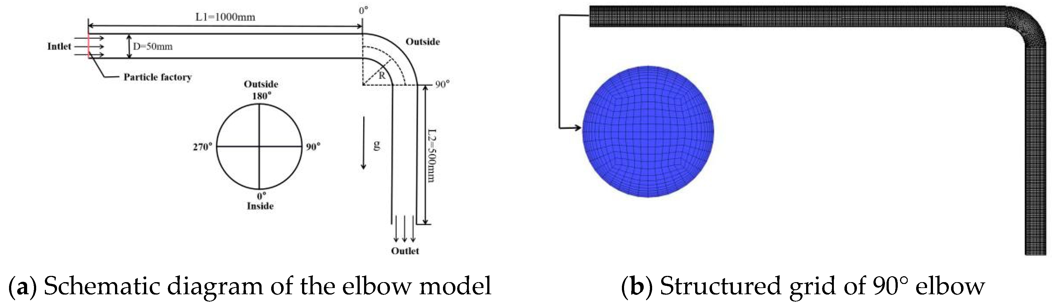
2.5. Verification of Erosion Model

Zeng et al. [26] used array electrode technology to measure the erosion rate at different positions of the X65 elbow. The geometric model consistent with the experiment is established in this paper, in which the pipe diameter (D) is 50 mm, the bending diameter ratio (R/D) is 1.5, the horizontal section (L1) is 20D, and the vertical section (L2) is 15D, as shown in Figure 4. Considering the secondary flow at the elbow, RNG k-ε is adopted as the turbulence model and the turbulence intensity is set to 3.5%. The height of the first boundary layer is 0.3 mm, the growth factor is 1.2, and the calculated Y+ range is 30~60. The calculation time step is set to 1 × 10⁻⁷ s in EDEM and 1 × 10⁻⁶ s in Fluent. The relevant parameters in EDEM and Fluent are shown in Table 2.
The comparison between the calculated erosion rate of the 90° elbow and the experimental results is shown in Figure 5. The corresponding azimuth angles of the outermost side and the symmetrical parts on the two outermost sides are defined as 180°, 130°, and 230°, respectively. As can be seen from the figure, the general trends of the simulation and experiment results are close, and the erosion rate at the elbow outlet is the largest, illustrating the correctness of the E/CRC erosion model adopted in this research.

3. Geometric Model and Boundary Conditions

3.1. Numerical Model Establishment

The research object of this paper consists of a standard tee junction and straight inlet and outlet pipes with a diameter of 30 mm. In order to obtain a stable two-phase velocity field before the liquid–solid mixture enters the tee junction, a vertical pipe with a length of 10D is set before the entrance of the tee junction. In order to eliminate the influence of the secondary flow in the tee pipe and obtain a stable pressure outlet, the length of the horizontal pipe at the outlet of the tee junction is also set to 10D. A cylindrical particle factory with a diameter of D and a length of 2D is built at the inlet of the vertical pipe, and the required particle concentration is simulated by setting the number of particles produced per second. The schematic geometric model is shown in Figure 6.
The computational domain of the tee pipe is divided by a structured grid. In this paper, the two-way coupling calculation approach is used, the particle volume fraction needs to be calculated, and the grid size is required to be 2–3 times the particle size. Considering the destructive effect of particles on the boundary layer and the calculation accuracy of the particle volume fraction at the boundary layer, the thickness of the first grid layer is 0.5 mm, and the value of Y+ is around 120.

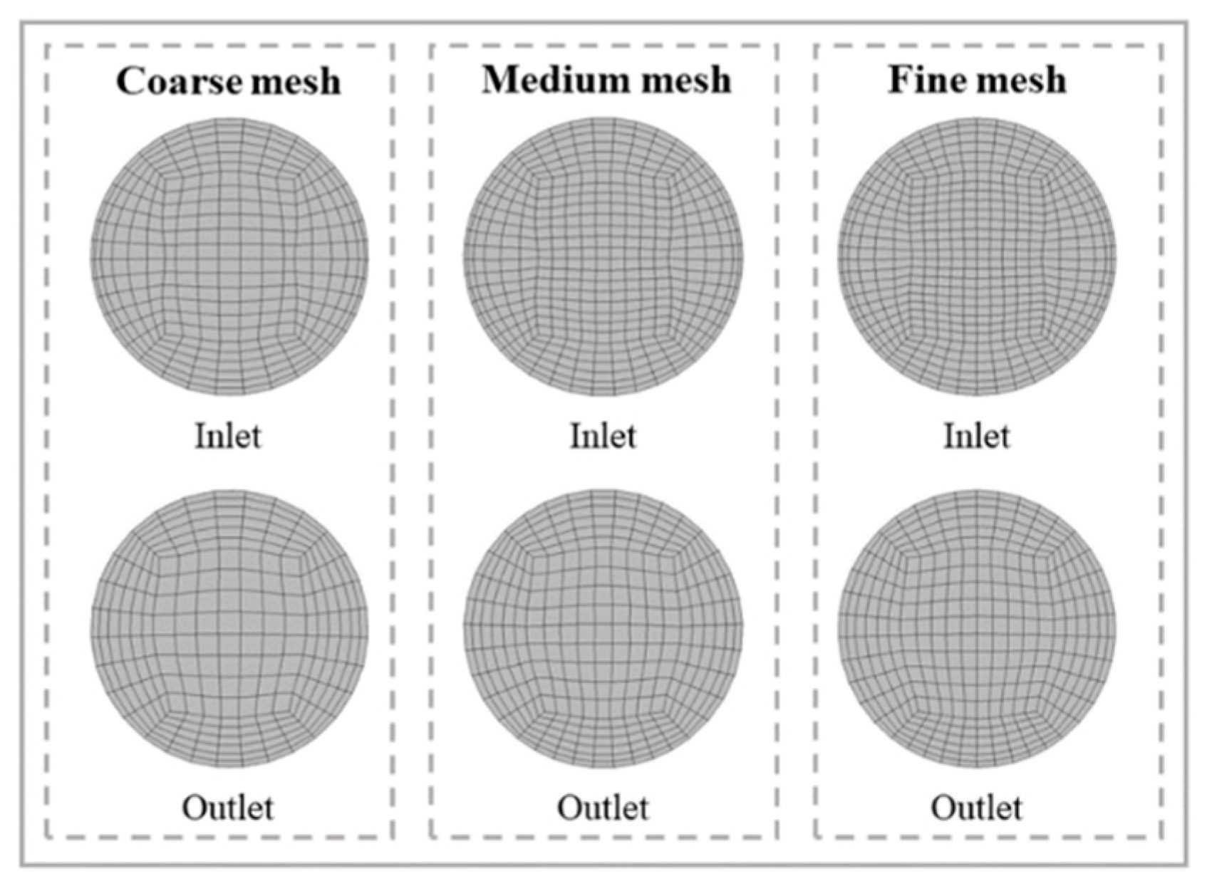
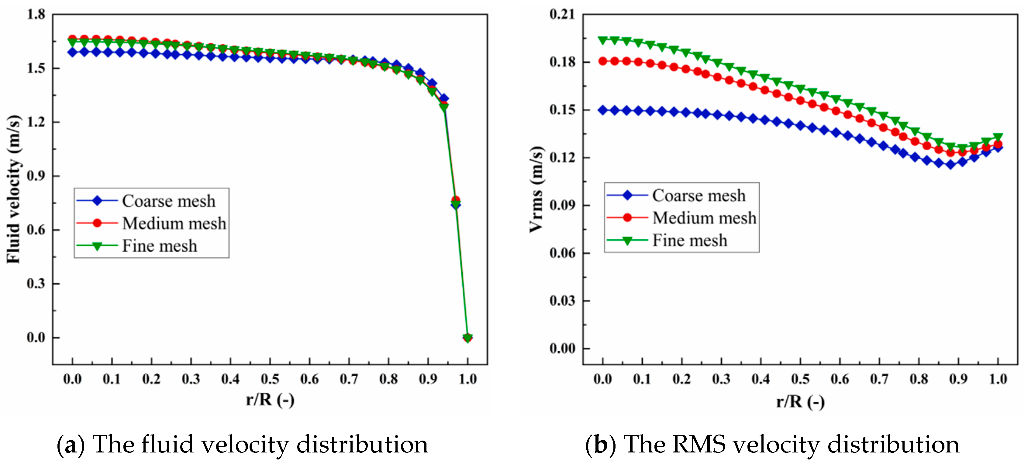
3.2. Independence Verification of Mesh

The Monte Carlo approach is adopted in this research to calculate the volume fraction of the particles, which requires the minimum volume of mesh to be 10 times the volume of the particle. For the fine mesh, during the CFD-DEM two-way coupling calculation process, it is easy to cause divergence in the numerical simulation. Therefore, the irrelevant research on the mesh is mainly reflected in the recognition of the mesh on the clear water flow field, as shown in Figure 7 and Table 3. The maximum relative error between the coarse mesh and the medium mesh is 4.2%, and the maximum relative error between the fine mesh and the medium mesh is 0.6%, as shown in Figure 8. Based on the above results, medium mesh is calculated in the following numerical simulation process.

3.3. Boundary Condition Settings

The inlet of the tee pipe is set as a velocity boundary condition of 3 m/s, the outlet is set as a pressure outlet with a reference pressure of 1 atm, and the wall of the tee pipe is set as a nonslip wall. Due to the secondary flow in the tee junction, the RNG k-ε turbulence model is selected, and the SIMPLE algorithm is adopted to couple the velocity and pressure field in the calculation of Fluent and EDEM. The Hertz–Mindlin (no slip) contact model is employed to calculate the particle–particle and particle–wall contact, and the E/CRC erosion model is adopted to calculate the erosion depth caused by solid particles. The flow field information in Fluent and the particle and wall parameters in EDEM are shown in Table 4.
During the coupling process of Fluent and EDEM, the Fluent calculation time step is an integer multiple of the EDEM calculating time step. The EDEM time step is 20% to 40% of the Rayleigh time step, and the formula of the Rayleigh time step is as follows:
t R = π R i 0.1631 v i + 0.8766 2 ρ p ( 1 + v i ) Y i
In the formula, Y i = 1 × 10 7 , R i = 1   m m , and v i = 0.17 represent the size of the Young’s modulus, radius, and Poisson’s ratio, respectively. Considering the calculation time and calculation accuracy, the EDEM calculation time step is 5 × 10⁻⁶ s, and the FLUENT calculation time step is 5 × 10⁻⁵ s.

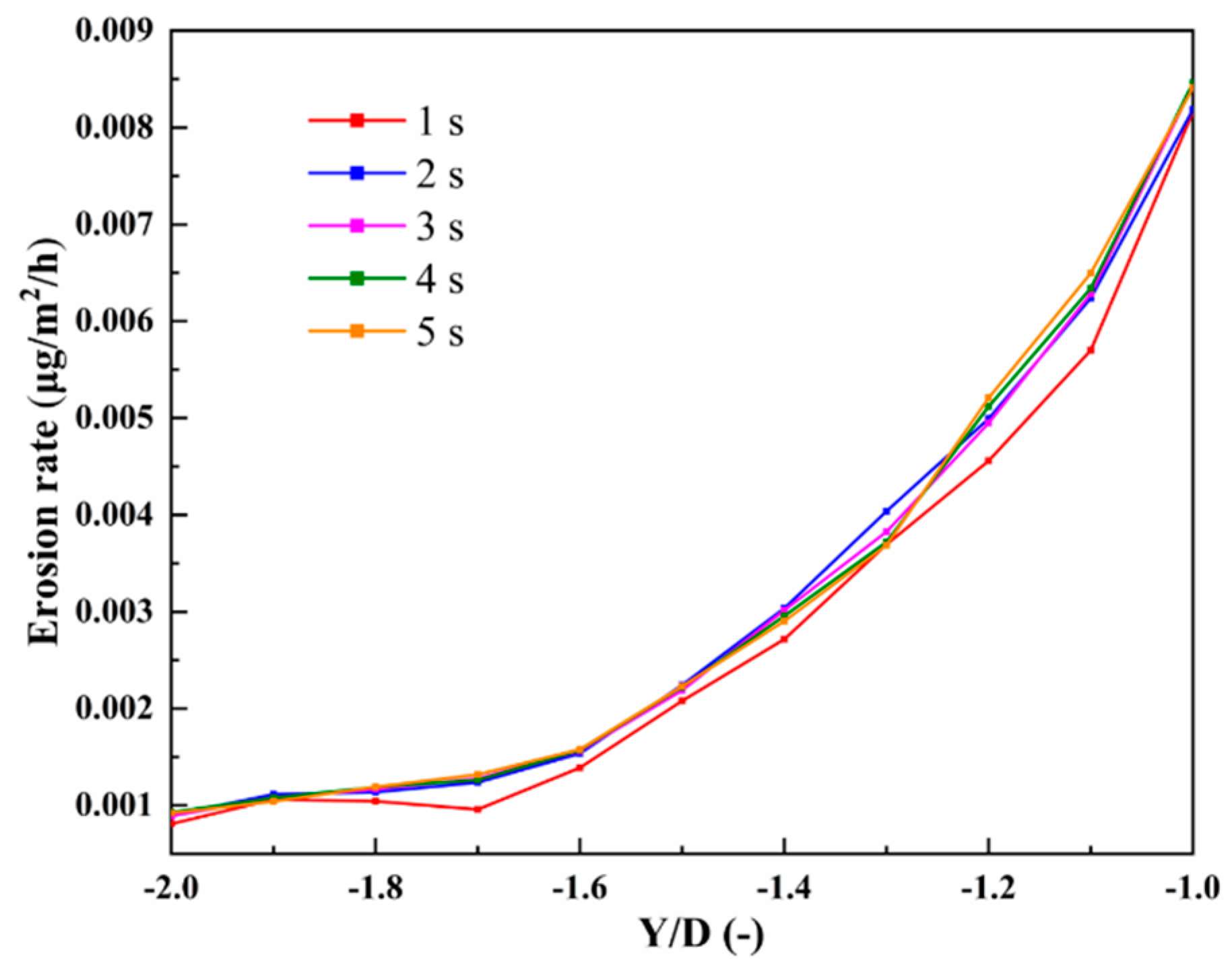
3.4. Independence Verification of Calculation Time

The main research content of this article is the erosion distribution caused by particles on the wall surface under the conditions of liquid–solid multiphase flow. Considering the insufficiency of the interaction between particles and fluid at the beginning, and the randomness of the particle position generated by the particle factory, there is a time statistics error on the wall erosion. Therefore, under the flow conditions of a particle diameter of 1 mm and a particle volume concentration of 0.5%, an irrelevant verification of calculating duration was performed. The erosion rate was average, and the erosion rate of the partial left branch pipe is shown in Figure 9. The results indicate that the simulation time has little influence on the prediction of the erosion distribution. Considering the calculation accuracy and computing resources, the calculation duration is 2 s.

4. Results and Discussion

4.1. Distribution of Cross-Sectional Velocity

In order to better understand the flow characteristics and erosion mechanism in the tee pipe, several sections are selected in the horizontal pipe, which are y = 15 mm, 30 mm, 45 mm, 105 mm, 150 mm, and 195 mm (named l1, l2, l3, l4, l5, and l6, respectively) under different working conditions, and the velocity distribution is extracted, as shown in Figure 10.
Although the geometric structure of the tee pipe is simple, the flowing process inside the tee pipe is complex and the velocity distribution changes drastically. For better analysis of the generation and development of vortices in the tee pipe, the contours of liquid velocity and the streamlines of liquid in six cross-sections downstream of the tee junction based on Case IG-0.5C-1D-5V were acquired, as shown in Figure 11.
The velocity gradient and the streamlines along the vortex coreline can be obviously observed. The region of high velocity presents a “crescent” shape, while the region of low velocity presents a “drop” shape. With the fluid flowing downstream, the high-velocity region becomes small, and the low-velocity region gradually moves up. When the fluid arrives at the outlet pipe, the velocity distribution tends to be uniform. Since the flow direction of the liquid changes at the tee junction, the flowing process of liquid in the outlet branch pipe becomes complex. Consequently, the streamlines of liquid in six cross-sectional positions were obtained to analyze the emergence and development of vortices. As shown in Figure 11a, when the fluid enters the tee junction from the vertical straight pipe, no vortex is generated. Then, in Figure 11b, two neighboring vortices in opposite directions arise in a symmetrical manner close to the side wall when the fluid passes through the tee junction. In addition, on Figure 11c,d, the two opposite vortices grow larger and progressively reach the center of the pipe. Eventually, in the y = 5D downstream position, the two vortices keep developing near the high-flow area and move closer to each other, as shown in Figure 11e,f.
For better understanding of the velocity distribution in the tee pipe under different working conditions, a cross-sectional velocity comparison of l4 under different inlet velocities, concentrations, and particle diameters was carried out. As can be seen from Figure 12, Figure 13 and Figure 14 the velocity contour distribution changes greatly under different flow conditions and, as the inlet velocity increases, the low-velocity region in the horizontal pipe becomes smaller and moves toward the center, while the high-velocity region becomes larger and diffuses circumferentially along the pipe wall. However, when the particle concentration increases, the high-velocity region does not change significantly, and the low-velocity region becomes wider and moves toward the pipe center. In addition, variations in particle size have little influence on the velocity distribution. This illustrates that the fluid velocity and particle concentration have a greater effect on the tee pipe transportation process.

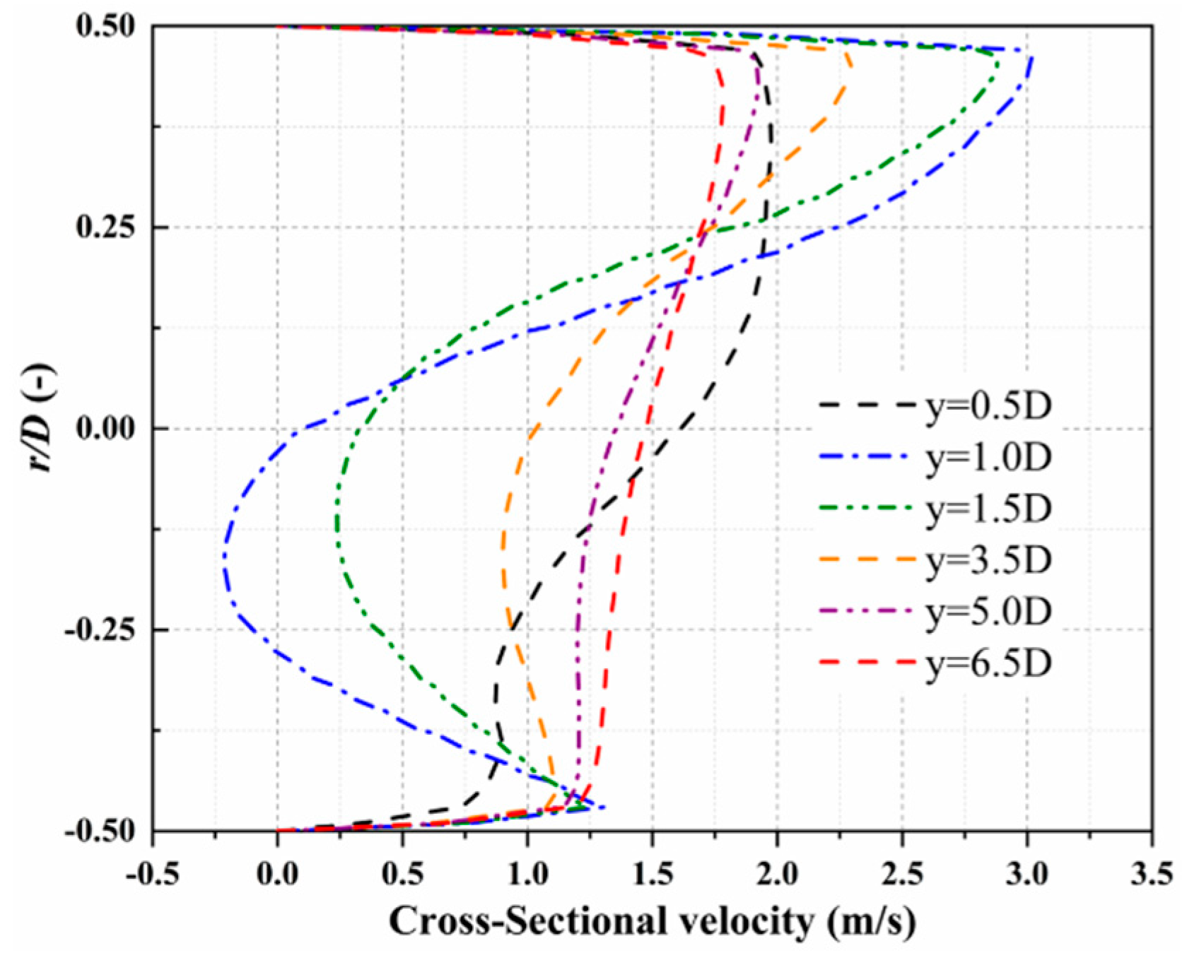
4.1.1. Cross-Sectional Velocity Profiles under Clean Water Conditions

The cross-sectional velocity distribution of Case OG-3V in the horizontal tee pipe under clean water conditions is shown in Figure 15, which provides some understanding of the flowing process downstream of the tee junction. It is obvious that the cross-sectional velocity distribution does not exhibit a parabolic shape such as the fully developed flow in a laminar pipe [27] due to the existence of the tee junction that generates flow circulations and vortices. At y = 0.5D, the velocity divergence between the upper and lower sides of the pipe is relatively small, since the fluid has just entered the tee junction and the flow separation has not yet occurred. Meanwhile, at y = 1.0D, the cross-sectional velocity presents significant changes, which are caused by the backflow and secondary flow. It reveals a considerable effect of the tee junction on the downstream flowing process, which enhances the interference with the completely developed incoming stream. Finally, the velocity distribution becomes increasingly consistent within the scope of y = 3.5D and 6.5D.

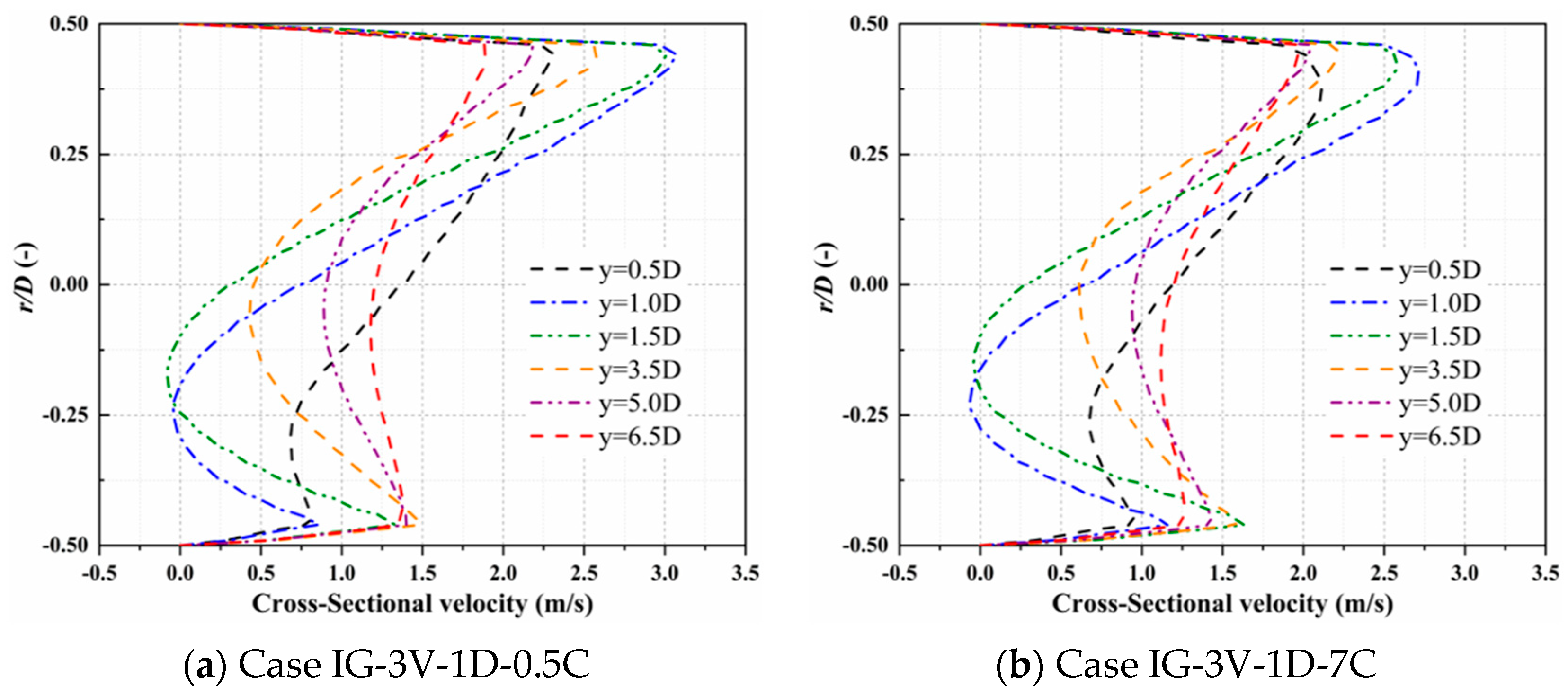
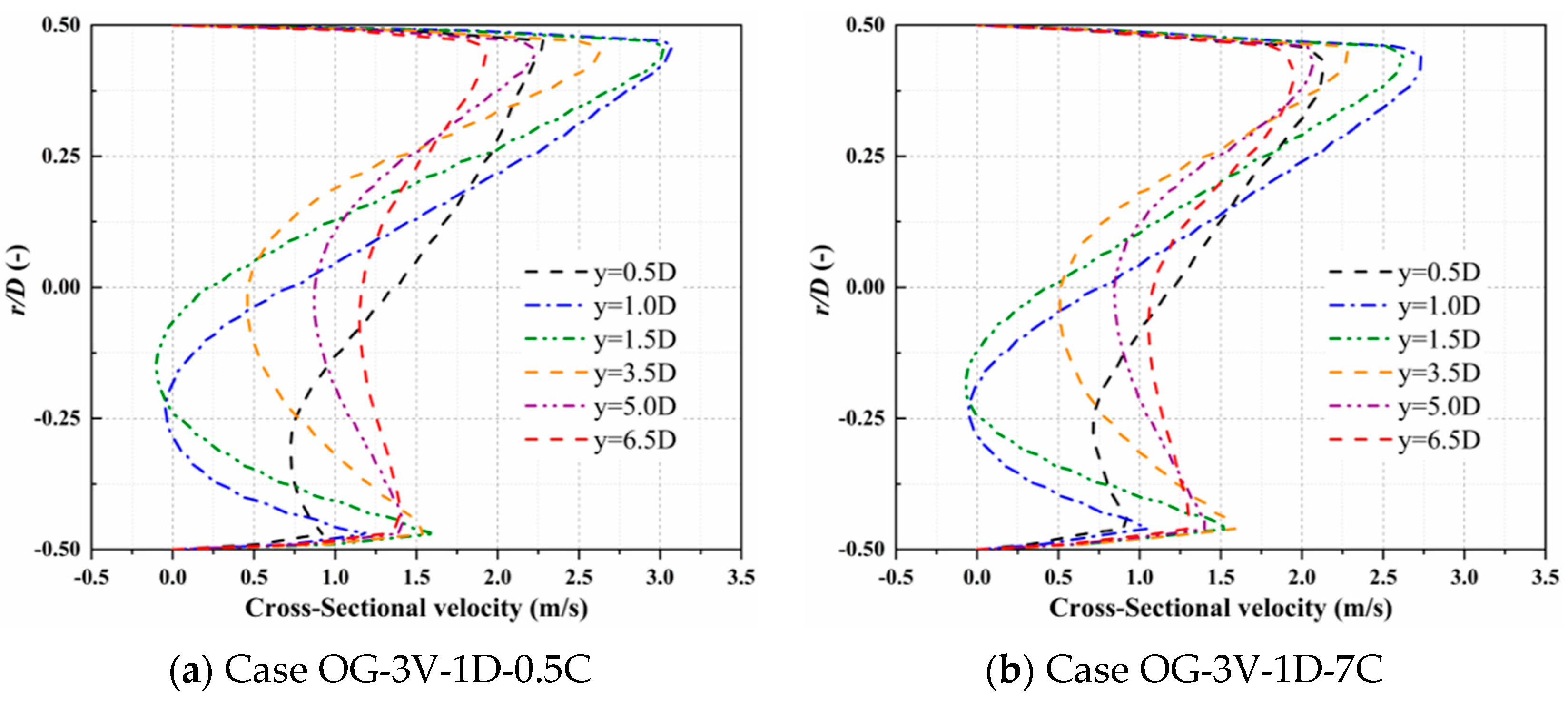
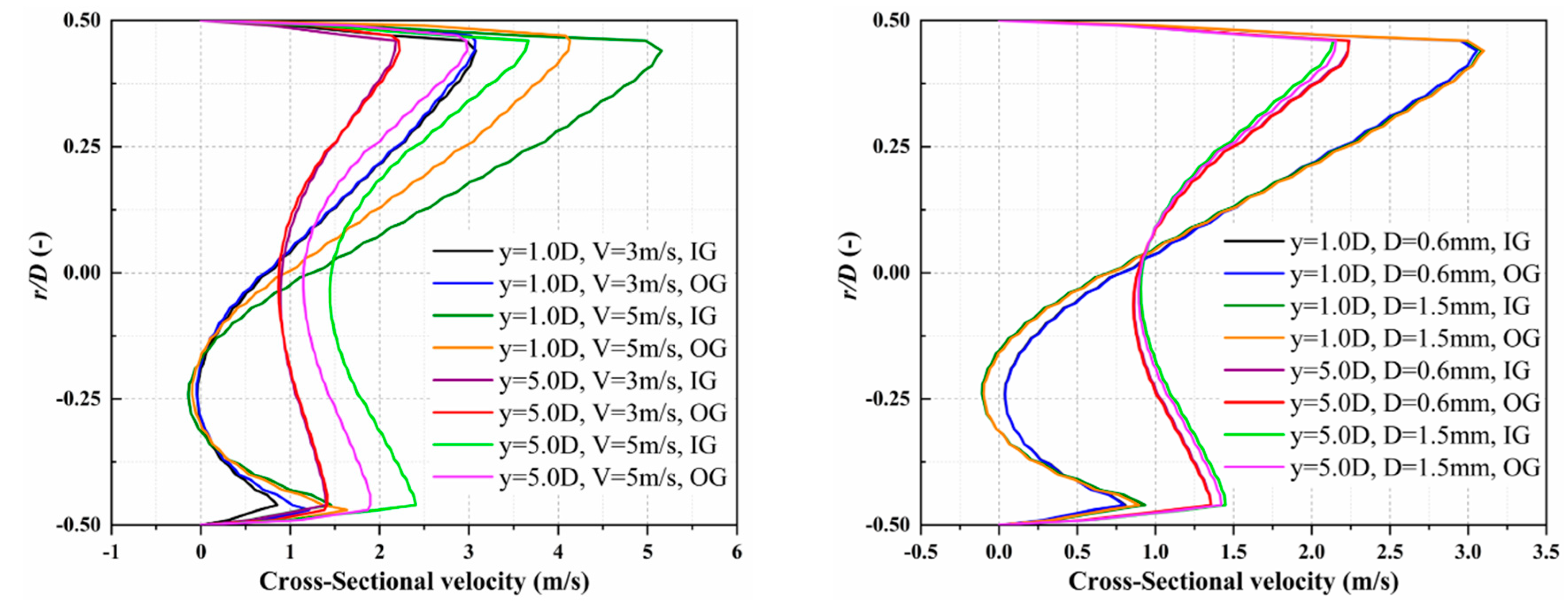
4.1.2. Cross-Sectional Velocity Profiles under Case IG-3V-1D and Case OG-3V-1D

In order to understand the influence of particle volume concentration on the fluid velocity distribution in the horizontal tee pipe, the cross-sectional velocity profiles under Case IG-3V-1D-0.5C, Case IG-3V-1D-7C, Case OG-3V-1D-0.5C, and Case OG-3V-1D-7C were found. Compared with Case OG-3V under clean water conditions, the cross-sectional velocity distribution tends to be roughly the same, and the velocity profile at y = 1.0D is moderated since the backflow phenomenon is suppressed to a certain extent. This is because the existence of particles in the pipeline changes the trajectory of the fluid and rectifies the fluid, eliminating part of the vortex under the clean water conditions.
It can be seen from Figure 16 and Figure 17 that the direction of gravity has little effect on the velocity distribution in the tee pipe since the cross-sectional velocity profiles are nearly the same. The velocity profiles of Case 3V-1D-0.5C and Case 3V-1D-7C at y = 1.0D and y = 5.0D are extracted in Figure 18 to compare the differences more clearly. When the particle volume concentration increases from 0.5% to 7%, the change in the high-speed area is more obvious, and the maximum fluid velocity becomes smaller. In addition, the difference in cross-sectional velocity becomes smaller as the fluid moves downstream.
The average velocity comparison of tee pipes has been made in Figure 19 with particle concentration increasing from 0.5% to 7% to analyze the influence of the two gravity directions on the flowing process when the fluid passes through the tee junction. It demonstrates the tendency of how the average cross-sectional velocities at different positions of the horizontal branch pipe (i.e., y = 1.0D, 5.0D, and 6.5D) change with the increase in particle concentration in the two gravity directions. It can be seen from the comparison that the variation tendency of the average velocity at different cross-sections downstream of the tee junction opposite to the gravity direction is consistent with that of the pipe identical to the gravity direction. It indicates that, for different gravity directions, the mainstream characteristics of the horizontal branch pipe downstream of the tee junction remain the same. Based on the particulars of profiles, the velocities at y = 1.0D in the OG direction cases are larger than that of the corresponding cases in the IG direction. The average cross-sectional velocity divergences between the two gravity directions become not obvious at y = 5.0D and y = 6.5D. It illustrates that the effect of the gravity direction mainly influences the flowing process close to the tee junction, which is progressively decreased and disappears along the horizontal branch pipe downstream of the tee junction.

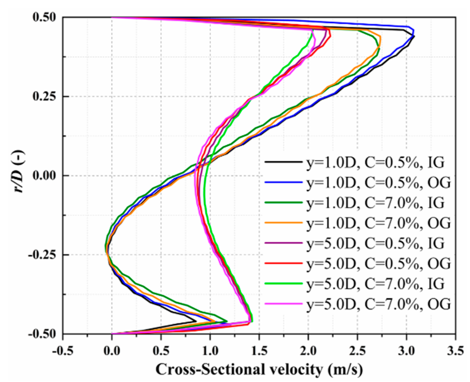
4.1.3. Cross-Sectional Velocity Profiles under Case 0.5C-1D and Case 3V-0.5C

It can be seen from Figure 20 that the cross-sectional velocity profiles are almost the same at 3 m/s under different gravity directions, while there are big differences at 5 m/s. This illustrates that the direction of gravity has a large effect on the velocity distribution in the tee pipe when the velocity is high. Meanwhile, the direction of gravity has little effect on the velocity distribution in the tee pipe under different particle diameters.

4.2. Analysis of Tee Pipe Erosion

In order to precisely identify how the erosion distribution of the tee pipe changes under different working conditions, including the direction of gravity, conveying parameters, and particle properties, the maximum erosion rate and the erosion distribution for the inner wall of the horizontal section from −5D to 5D are acquired. Different from common knowledge, the region with the most severe erosion does not occur at the upstream wall of the center of the horizontal section facing the vertical pipe. On the contrary, the position y/D = 0 in the middle of the upstream wall is a low-erosion region, and the region with the most severe erosion and wear occurs at the position y = 0.75D on both sides of the center. In other words, for most tee junctions which consist of one vertical main pipe and two horizontal branch pipes, the most severe erosion appeared approximately three fourths of the pipe diameter away from the tee junction. Through a series of measurement experiments on the erosion depth of the tee pipes under different flow conditions, it is found that the thinnest region is located at horizontal branch pipes downstream of the tee junction, and the distance between the most severe erosion region and the tee junction center is about three fourths of the pipe diameter, which proves the accuracy of the numerical simulation.

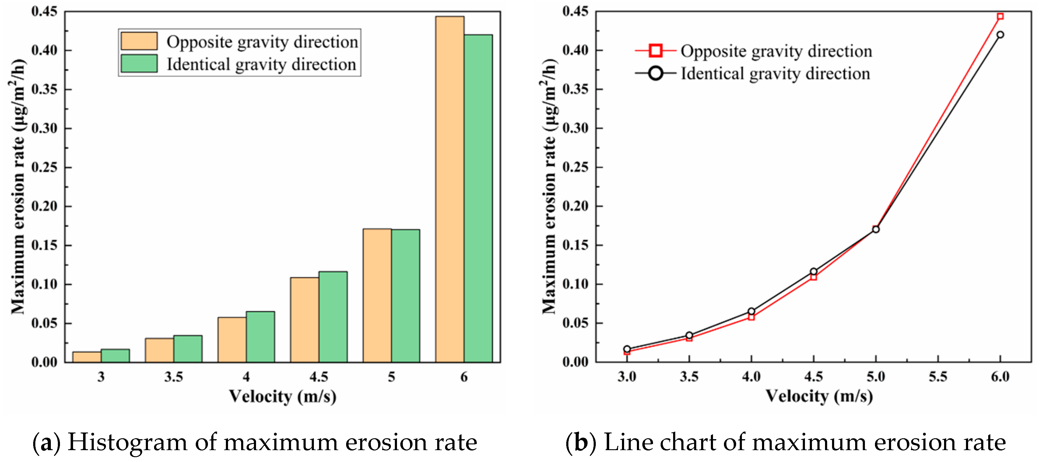
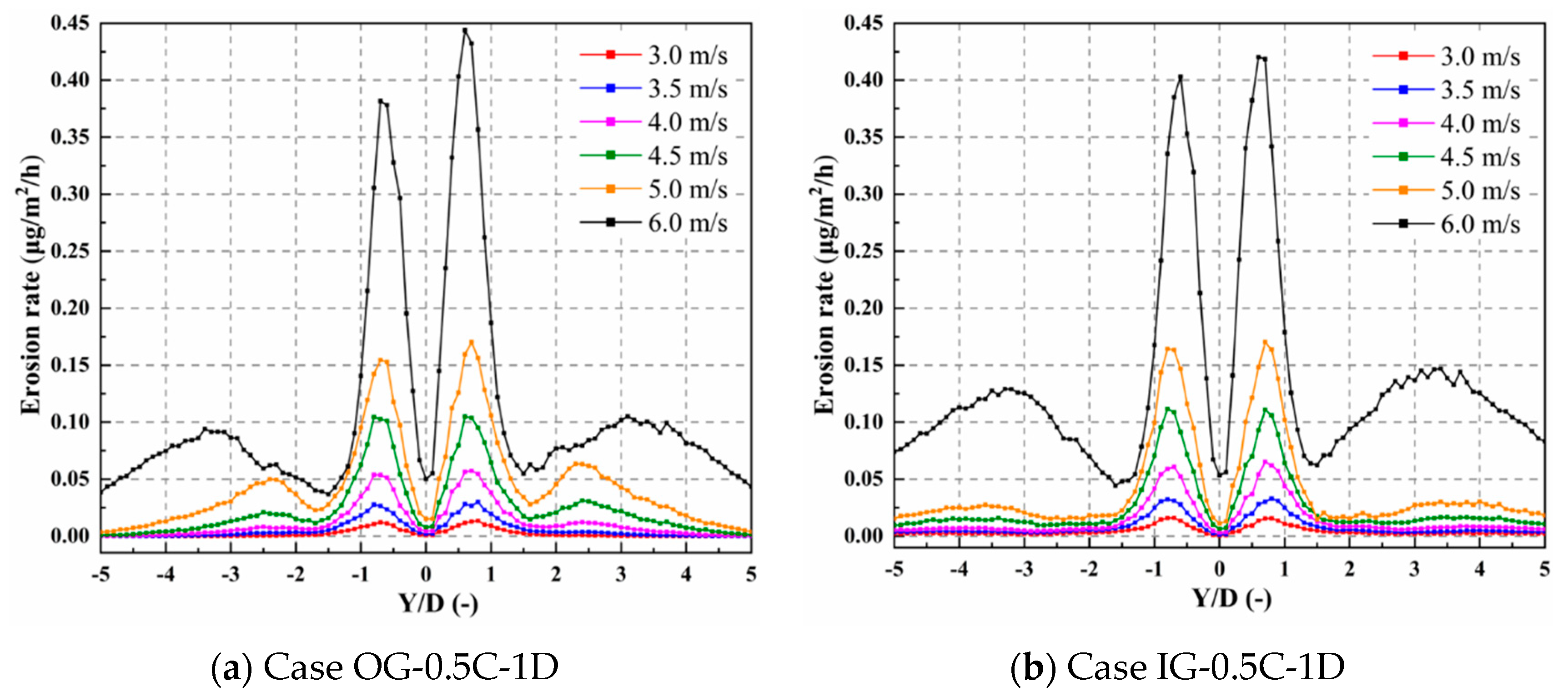
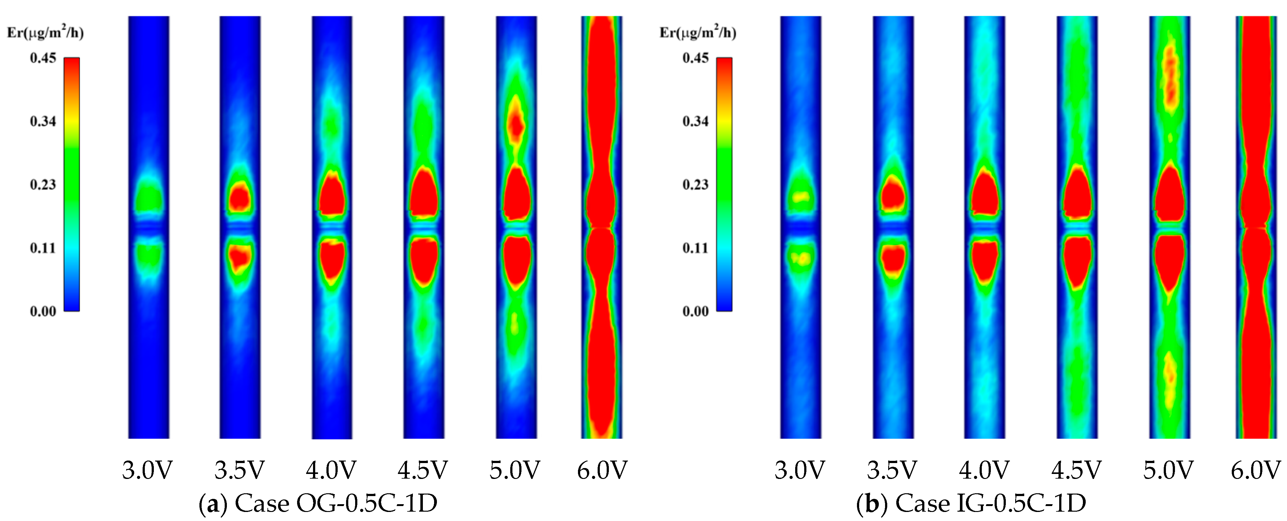
4.2.1. Effect of Inlet Velocity

Different conveying velocities are often adopted in pipeline transportation according to the actual situation on site. Therefore, simulations of tee pipes regarding the erosion characteristics with different velocities are carried out under the same particle diameter of 1 mm and particle volume concentration of 0.5%. By changing the initial inlet velocity of fluid and particles, the relationship between the erosion rate and the conveying velocity is obtained, as shown in Figure 21, Figure 22 and Figure 23.
As shown in Figure 21, when the conveying velocity increases, the maximum erosion rate of the pipeline increases and shows exponential growth. Since the kinetic energy of particle collision has a quadratic relationship with the velocity, the change in fluid velocity has a considerable impact on erosion. A higher inlet velocity will make the solid particles obtain greater collision energy, and the cutting effect generated by hitting the pipe wall will be stronger, leading to an increase in the erosion rate. Comparing the two curves in Figure 21b, it can be found that when the inlet velocity is lower than 5 m/s, the growth rate of the maximum erosion rate of Case IG-0.5C-1D is slightly greater than that of Case OG-0.5C-1D, which is due to the impact of gravity. The kinetic energy of the particles in the pipeline in the IG direction is slightly greater than that in the OG direction, and the pipeline erosion is slightly stronger. When the inlet velocity is higher than 5 m/s, the erosion growth rate in Case OG-0.5C-1D exceeds that in Case IG-0.5C-1D, because as the velocity increases, some particles cannot follow the mainstream in time and are attached to the wall by gravity, which blocks the impact of particles in the subsequent incoming flow and slows down the erosion process.
When the direction of gravity is opposite to the inlet velocity, the erosion from the middle position of the horizontal pipeline to the outlet on both branch pipes presents two peaks and one trough, as shown in Figure 22a. The position of y = 0.75D is the main erosion peak, and the erosion rate of the pipe inner wall reaches the maximum value, while the position of y = 1.5D is the erosion trough, and the erosion rate is relatively small. When the velocity is lower than 5 m/s, the secondary erosion peak appears at the position y = 2.5D. However, the secondary erosion peak shifts to the position y = 3.5D when the velocity increases to 6 m/s. The erosion rate gradually decreases along the outlet direction outside the secondary erosion peak. The main erosion peak is caused by the direct collision of the particles carried by the mainstream fluid in the vertical pipe on the facing wall, and the secondary erosion peak is caused by the secondary flow and backflow formed in the branch pipe through the tee junction. When the gravity direction is the same as that of the inlet velocity, the variation tendency of the erosion rate in the main erosion region is close to Case OG-0.5C-1D as the inlet velocity increases from 3 m/s to 5 m/s, while the secondary erosion peak is not obvious, and the change in erosion rate on both sides of the branch pipes tends to be stable. This indicates that under the condition of low inlet velocity, the erosion of the pipeline in the IG direction is less affected by the secondary flow. However, when the velocity reaches 6 m/s, the erosion rate in the secondary erosion peak region changes significantly, widens, and shifts to the outlets on both sides of the branch pipes. At the position y = 5D, the erosion rate of the pipeline increases significantly, indicating that the erosion downstream is more severe. It can be seen that with the increase in the conveying velocity, the impact of the secondary flow and backflow in the pipeline on the erosion is significant.
Figure 23a and Figure 23b, respectively, show the erosion contours of Case OG-0.5C-1D and Case IG-0.5C-1D. It can be seen from Figure 23 that two erosion regions appear in pairs at the branch pipes under the velocities of 3 m/s and 3.5 m/s, which correspond to the main erosion peaks. When the velocity increases to 4 m/s, the secondary erosion regions start to appear on both sides of the main erosion region. As the velocity increases to 6 m/s, the erosion regions gradually become larger and wider. The erosion strength under the condition of Case IG-0.5C-1D seems to be more severe and there is a continuous erosion region from the branch pipe center to the outlet, while there is a discontinuous erosion region outside the main erosion region under the condition of Case OG-0.5C-1D.

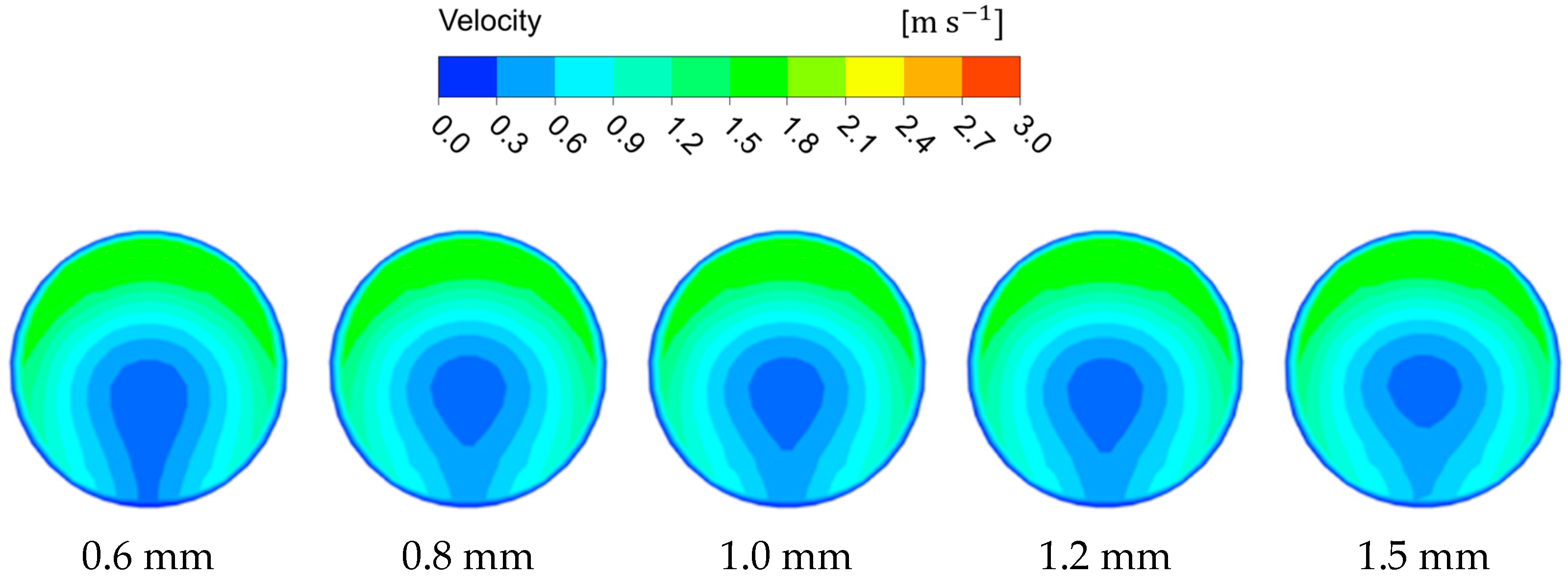
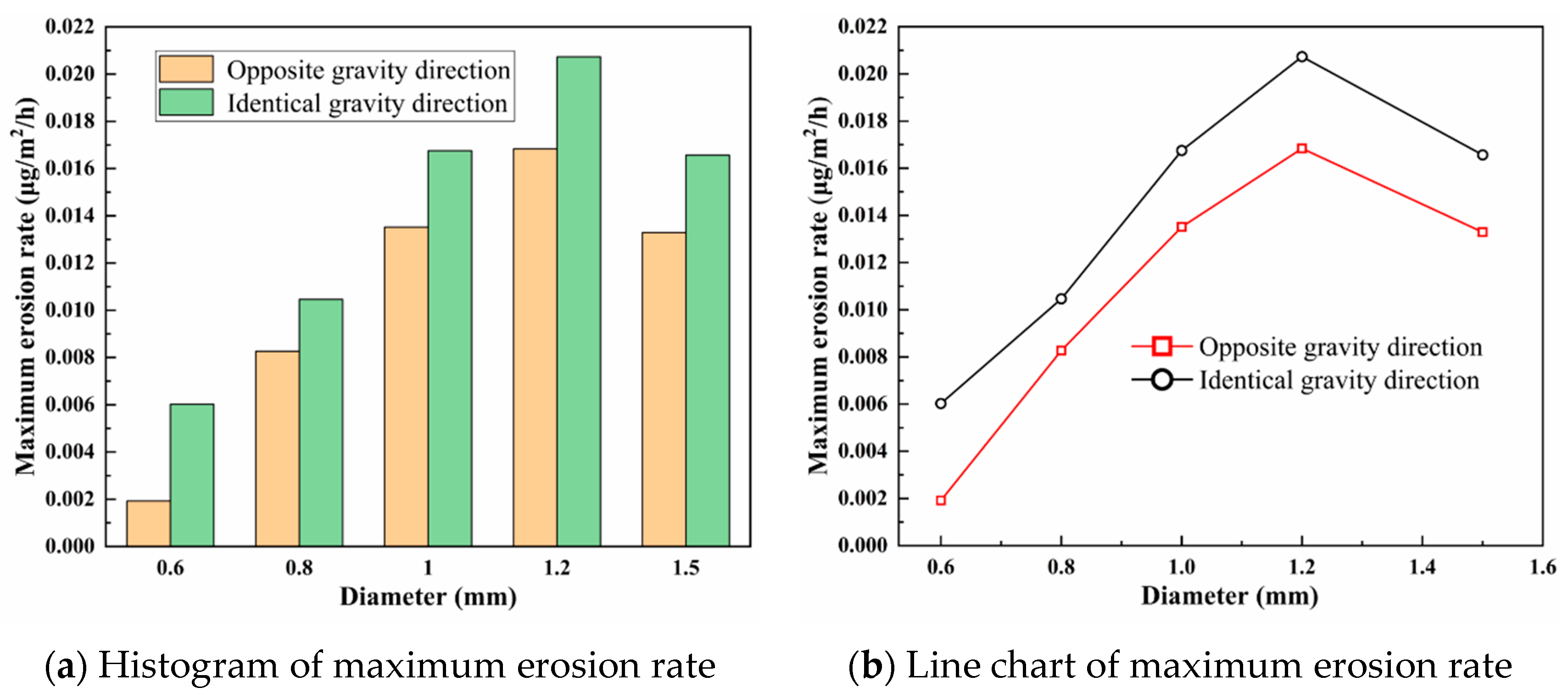
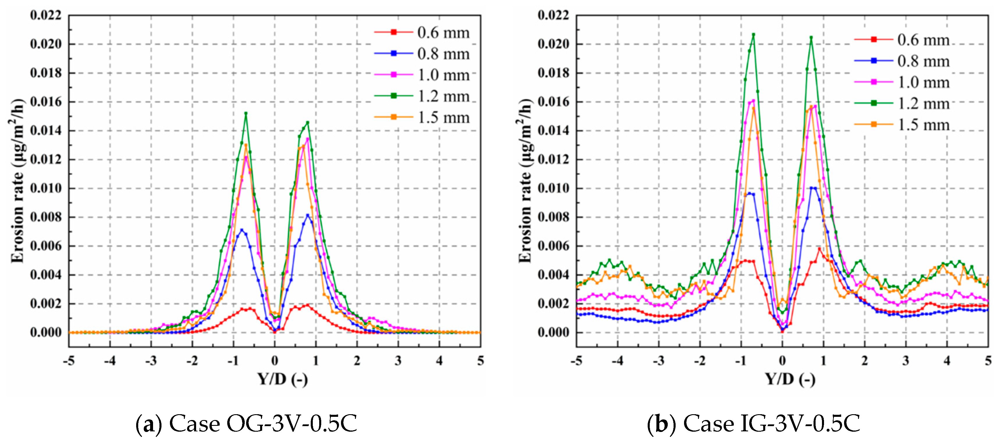
4.2.2. Effect of Particle Diameter

Since the shape and size of solid particles are different in the process of pipeline transportation, erosion caused by particles with different diameters changes accordingly. Assuming that the particle velocity is 3.0 m/s and the particle volume concentration is 0.5%, the relationship between the erosion rate and the particle diameter can be obtained by changing the particle velocity, as shown in Figure 24, Figure 25 and Figure 26.
When the particle diameter increases from 0.6 mm to 1.5 mm, the maximum erosion of the pipeline first increases and then decreases, as shown in Figure 24. With the particle diameter increasing, the mass of a single particle increases, thereby increasing the kinetic energy, and the erosion caused by the particle hitting the wall is strengthened. Since the particle Stokes number represents the ratio of the particle response time to the flow field change and the fluid characteristic time, when the particle diameter increases, the inertial force correspondingly increases, and the time for the particles to respond to changes in the flow field increases. At this time, the particles are less affected by the fluid flow, the flowability of the particles becomes worse, thus the erosion on the pipe inner wall is weakened.
When the direction of gravity is opposite to the inlet velocity, there is an erosion peak from the middle of the horizontal pipe to the outlet on both branch pipes. Outside the y = 3D position, the erosion rate is relatively minimal and tends to be stable. Due to the action of gravity, the particles bounce back to the mainstream area after colliding with the inner wall, and follow the fluid to move downstream, so the collision frequency with the wall is reduced and the erosion is weakened. When the direction of gravity is the same as the inlet velocity, the erosion rate is higher under the same particle size and the erosion on the inner wall surface of branch pipes on both sides of the tee junction is obvious, because the particles in the main flow will hit the wall under the influence of fluid disturbance and gravity. In addition, the secondary erosion peak appears with a large particle size, since the Stokes number of large particles is relatively large, corresponding to the poor flowability, and the downstream of the horizontal pipe is less affected by the mainstream. Therefore, with the impact of gravity, large particles frequently hit the wall, forming erosion regions on both sides of the horizontal branch pipes.
Figure 26a and Figure 26b, respectively, show the erosion contours of Case OG-3V-0.5C and Case IG-3V-0.5C. As can be seen from the contours, with the increase in particle diameter, the area of the main erosion region firstly expands and then shrinks, and the maximum erosion rate value is reached at a 1.2 mm particle diameter. That is to say, 1.2 mm is the critical particle diameter in this working condition.

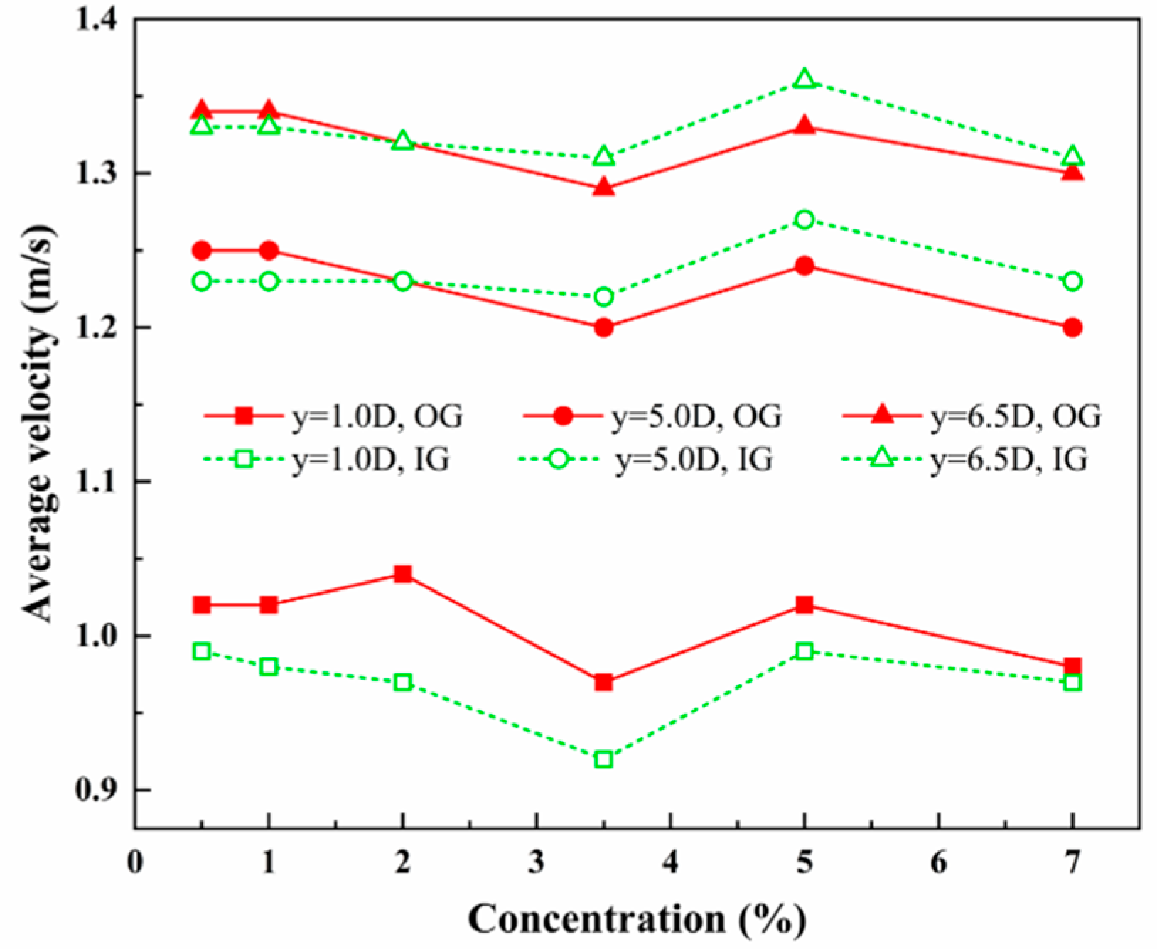
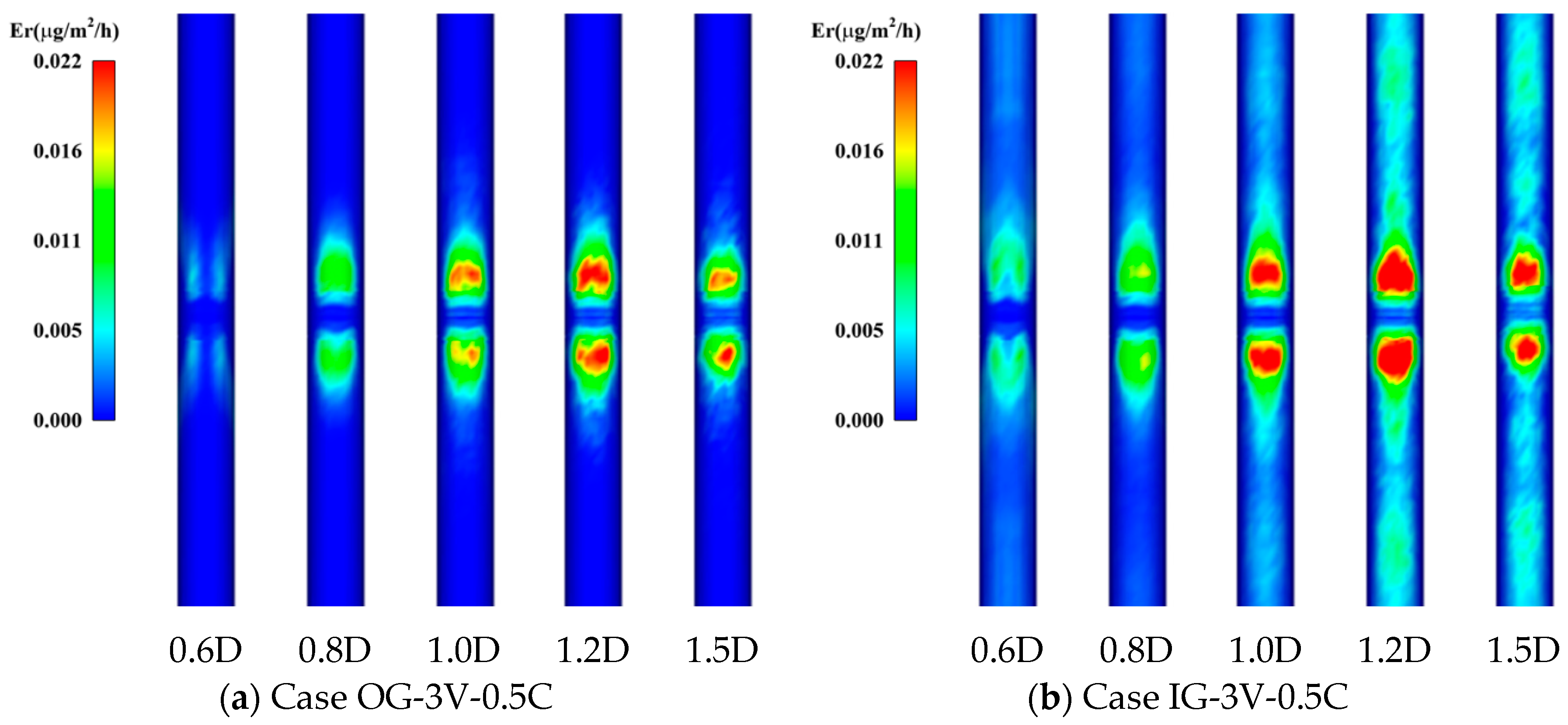
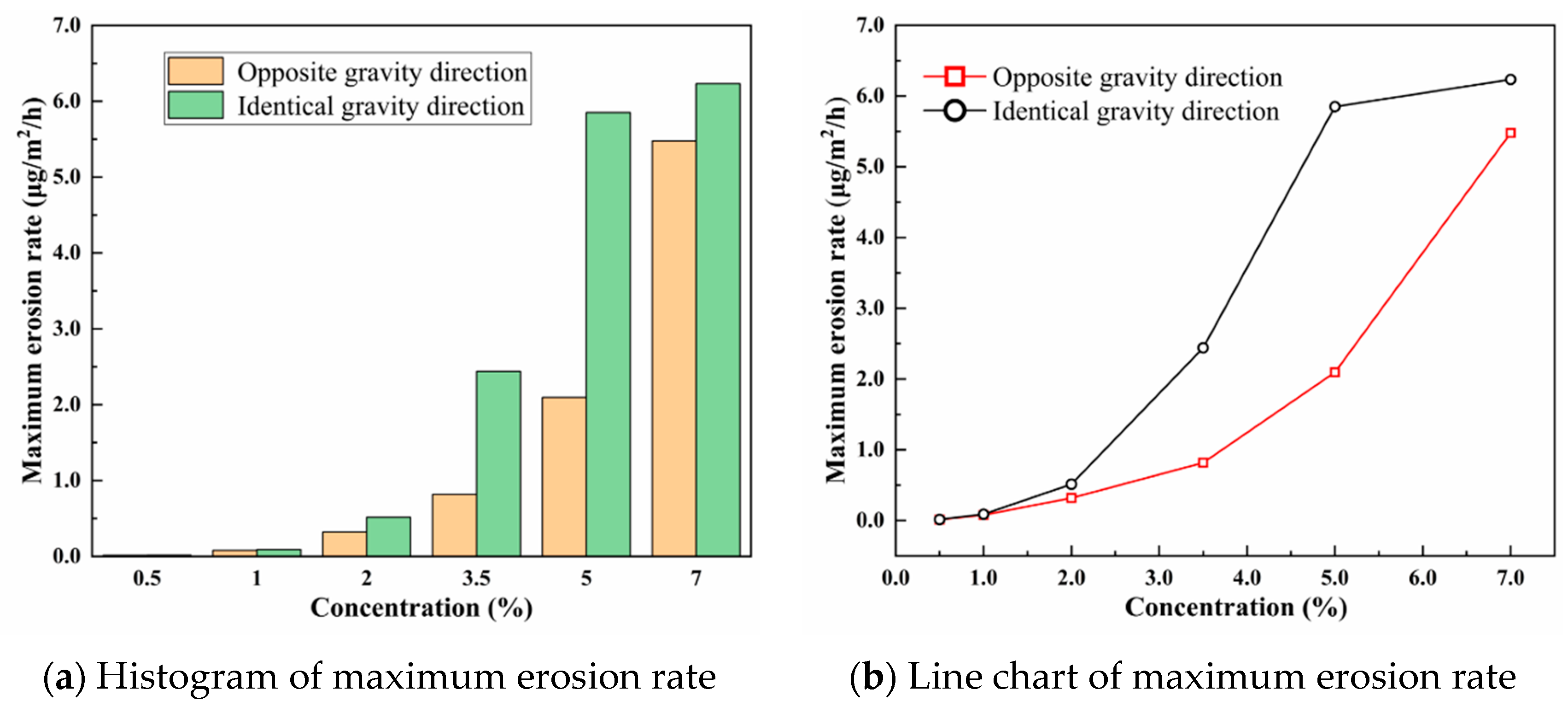
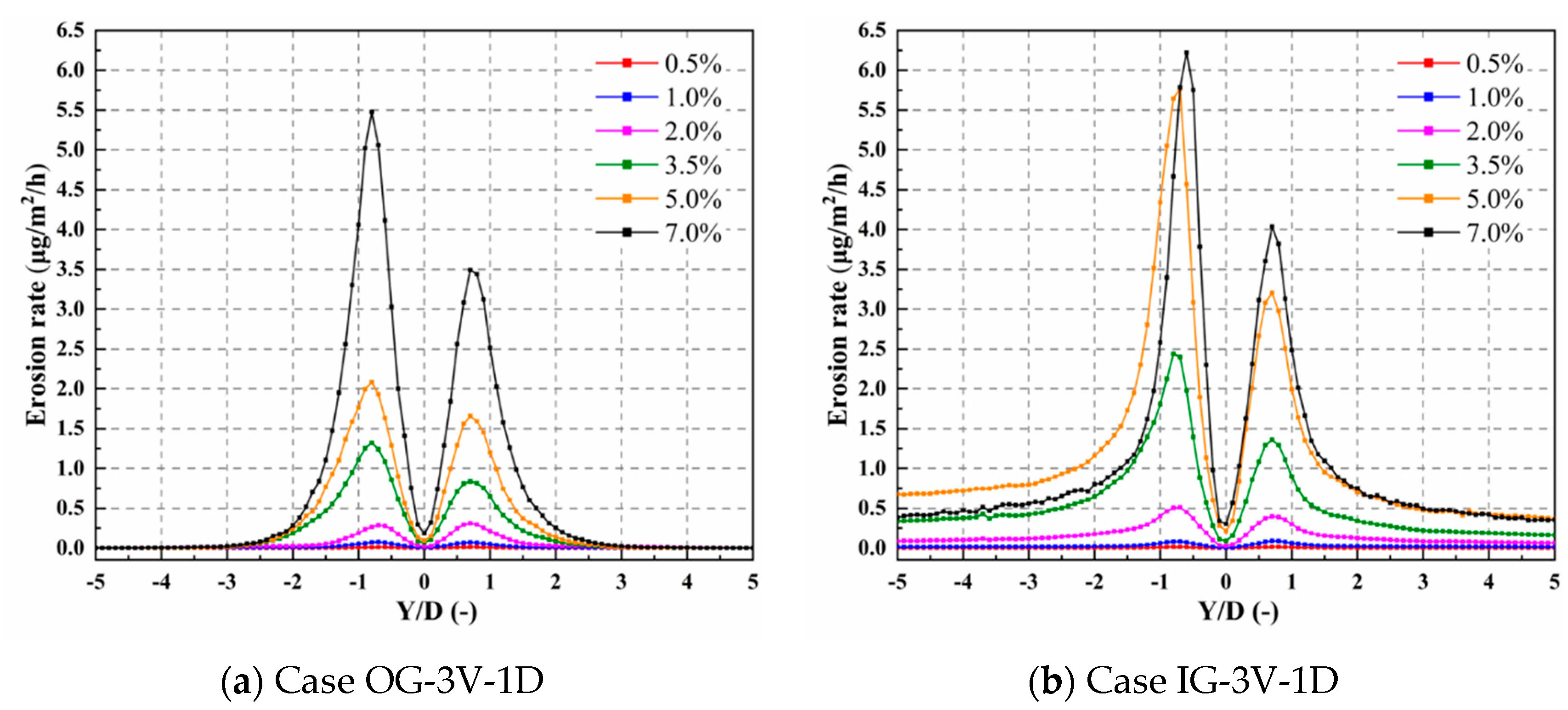
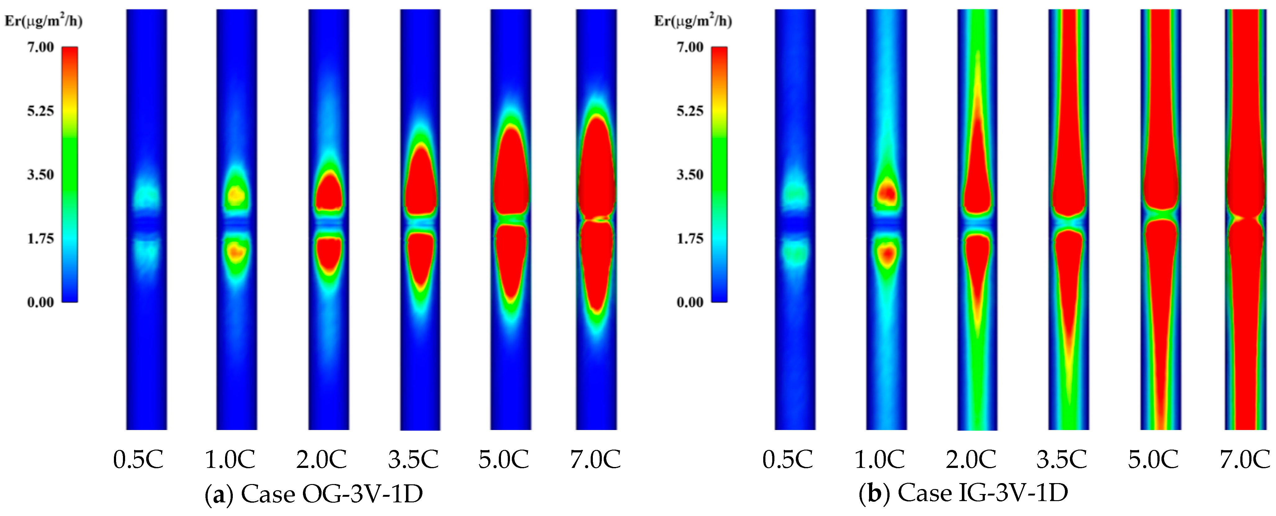
4.2.3. Effect of Particle Volume Concentration

Assuming that the particle diameter is 1.0 mm and the particle velocity is 3.0 m/s, the relationship between the erosion rate and the particle volume concentration can be obtained by changing the particle volume concentration, as shown in Figure 27, Figure 28 and Figure 29.
As shown in Figure 27, with the particle volume concentration increasing, the maximum erosion rate of the pipe inner wall increases exponentially, because the number of particles hitting the pipe wall per unit time increases, and the collision frequency of particles on the wall increases, resulting in a rapid growth in the erosion rate of the pipeline. One main erosion peak appears on both sides of the horizontal branch pipes.
When the direction of gravity is opposite to the inlet velocity, the erosion area is mainly concentrated at the position y = 0.75D, while the erosion rate is relatively small and negligible outside the position y = 3D. This is because the particles fall back to the mainstream after colliding with the wall under the action of gravity, so the impact frequency on the walls of the branch pipes on both sides is relatively small, and the erosion is weak. When the gravity direction is the same as the inlet velocity, the erosion rate of the pipeline increases significantly under the same particle volume concentration. When the particle volume concentration reaches 7.0%, the erosion growth rate is significantly reduced, and the erosion rate of some pipelines is less than that under the condition of 5% concentration. The erosion rate on both sides of branch pipes is much greater than that in Case OG-3V-1D, which is because the movement direction of the particles is the same as the gravity direction, the kinetic energy is relatively high, the cutting action of the particles hitting the pipe wall is enhanced, thus the erosion is increased. Furthermore, when the concentration is high, the collision between the particles becomes more intense, resulting in partial energy loss, causing the collision velocity with the pipe wall to decrease, thereby the erosion rate decreases. Affected by gravity, some particles accumulate and adhere to the facing wall surface, preventing further erosion and wear of the wall surface caused by particles in the subsequent incoming flow, that is why the erosion growth rate of the main erosion peak slows down. At the same time, the particles accumulated on the wall surface are squeezed and pushed by the fluid and particles, slide and collide with the wall surface, and translate to the outlet, showing a long wear belt on both branch pipes.
Figure 29 shows the distribution of the erosion region under different particle volume concentrations. As can be seen, the erosion region presents a conical shape and is located at the bottom of the tee junction, which is consistent with the position of the high-velocity area. The higher the particle volume concentration, the larger the conical erosion region of the tee pipe, because the growth of the particle number in the fluid leads to the corresponding increase in the tee pipe erosion degree. In addition, due to the influence of gravity, the conical region in Figure 29b is longer than in Figure 29a, indicating that the erosion in branch pipes is more severe.

5. Conclusions

Erosion in tee pipes under different gravity directions has been studied through numerical calculations. The main purpose of this research is to investigate the influences of gravity direction, conveying parameters, and particle properties on the erosion characteristics. The flow characteristics and erosion mechanism are discussed by analyzing the erosion distribution and velocity profiles in the tee pipes. The results indicate that the distribution of velocity and erosion rate varied greatly with different flow conditions.
As the fluid and particles move from the tee junction to the outlet, velocity contours and streamlines vary greatly at different cross-sections due to the complexity of the flow. With the fluid velocity and particle concentration increasing, the low-velocity region becomes smaller and moves toward the pipe center, while the particle diameter has little influence on the distribution of the low-velocity region. The direction of gravity has a nonnegligible influence on the cross-sectional velocity profiles, especially under the condition of high velocity and high particle concentration. For different gravity directions, the flowing process close to the tee junction is mainly affected, while the mainstream characteristics of branch pipes downstream the tee junction remain the same.
Different from common knowledge, the region with the most severe erosion occurred at the position y = 0.75D of branch pipes, about three fourths of the pipe diameter away from the tee junction and consistent with the experiment. With the conveying velocity increasing, the maximum erosion rate of the tee pipe increases and shows exponential growth. When the particle diameter increases from 0.6 mm to 1.5 mm, the maximum erosion rate first increases then decreases, and 1.2 mm is the critical diameter. With the particle volume concentration increasing, the maximum erosion rate first increases exponentially and then decreases when the gravity direction is identical to that of the inlet velocity. The main erosion peak is caused by the direct collision of the particles carried by the mainstream fluid on the facing wall, and the secondary erosion peak is caused by the secondary flow and backflow formed in the branch pipe through the tee junction.
For further studies, experimental data on the validity of this numerical method are required since the erosion is altered from different working conditions. At the same time, this approach will provide an effective analysis tool for better understanding the mechanism of liquid–solid multiphase flow in tee pipes and can be utilized to estimate the erosion characteristics downstream of the tee junction to prevent pipeline failure.

Author Contributions

S.H.: Conceptualization, Methodology, Software, Validation, Formal analysis, Investigation, Writing—original draft, Writing—review and editing, Visualization. G.P.: Conceptualization, Writing—review and editing, Resources, Project administration, Funding acquisition. D.Y. and H.C.: Conceptualization, Methodology, Investigation, Writing—review and editing, Supervision. X.W.: Conceptualization, Methodology, Investigation, Writing—review and editing, Supervision. All authors have read and agreed to the published version of the manuscript.

Funding

The authors gratefully acknowledge the support from Open Research Subject of Key Laboratory of Fluid Machinery and Engineering (Xihua University) (grant number LTDL2022006); Open Research Subject of Hubei Key Laboratory of Hydroelectric Machinery Design & Maintenance (China Three Gorges University) (grant number 2020KJX07); the 69th batch of general funding from the China Postdoctoral Science Foundation (grant number: 2021M691298); Natural Science Re-search Project of Jiangsu Province Colleges and Universities (grant number: 21KJB570004), Priority Academic Program Development of Jiangsu Higher Education Institutions (PAPD); the 22nd batch of college students’ scientific research projects to be funded (Jiangsu University) (grant number 22A232).

Institutional Review Board Statement

Not applicable.

Informed Consent Statement

Not applicable.

Data Availability Statement

Date are contained within the article.

Conflicts of Interest

The authors declare that they have no known competing financial interests or personal relationships that could have appeared to influence the work reported in this paper.

References

  1. Finnie, I. Erosion of surfaces by solid particles. Wear 1960, 3, 87–103. [Google Scholar] [CrossRef]
  2. Finnie, I. The Fundamental Mechanisms of the Erosive Wear of Ductile Metals by Solid Particles; Lawrence Berkeley National Laboratory: Berkeley, CA, USA, 1978. [Google Scholar]
  3. Bitter, J.G.A. A study of erosion phenomena part I. Wear 1963, 6, 5–21. [Google Scholar] [CrossRef]
  4. Bitter, J.G.A. A study of erosion phenomena: Part II. Wear 1963, 6, 169–190. [Google Scholar] [CrossRef]
  5. Archard, J.F. Contact and rubbing of flat surfaces. J. Appl. Phys. 1953, 24, 981–988. [Google Scholar] [CrossRef]
  6. Oka, Y.I.; Okamura, K.; Yoshida, T. Practical estimation of erosion damage caused by solid particle impact: Part 1: Effects of impact parameters on a predictive equation. Wear 2005, 259, 95–101. [Google Scholar] [CrossRef]
  7. Oka, Y.I.; Yoshida, T. Practical estimation of erosion damage caused by solid particle impact: Part 2: Mechanical properties of materials directly associated with erosion damage. Wear 2005, 259, 102–109. [Google Scholar] [CrossRef]
  8. Chen, X.; McLaury, B.S.; Shirazi, S.A. Effects of applying a stochastic rebound model in erosion prediction of elbow and plugged tee. Fluids Eng. Div. Summer Meet. 2002, 36169, 247–254. [Google Scholar]
  9. Edwards, J.K.; McLaury, B.S.; Shirazi, S.A. Modeling solid particle erosion in elbows and plugged tees. J. Energy Resour. Technol. 2001, 123, 277–284. [Google Scholar] [CrossRef]
  10. Wang, K.; Li, X.; Wang, Y.; He, R. Numerical investigation of the erosion behavior in elbows of petroleum pipelines. Powder Technol. 2017, 314, 490–499. [Google Scholar] [CrossRef]
  11. Huang, Y.; Zhu, L.; Liao, H.; Zou, D.; Wang, J. Erosion of plugged tees in exhaust pipes through variously-sized cuttings. Appl. Math. Model. 2016, 40, 8708–8721. [Google Scholar] [CrossRef]
  12. Zamani, M.; Seddighi, S.; Nazif, H.R. Erosion of natural gas elbows due to rotating particles in turbulent gas-solid flow. J. Nat. Gas Sci. Eng. 2017, 40, 91–113. [Google Scholar] [CrossRef]
  13. Chen, X.; McLaury, B.S.; Shirazi, S.A. Numerical and experimental investigation of the relative erosion severity between plugged tees and elbows in dilute gas/solid two-phase flow. Wear 2006, 261, 715–729. [Google Scholar] [CrossRef]
  14. Farokhipour, A.; Mansoori, Z.; Rasteh, A.; Rasoulian, M.A.; Saffar-Avval, M.; Ahmadi, G. Study of erosion prediction of turbulent gas-solid flow in plugged tees via CFD-DEM. Powder Technol. 2019, 352, 136–150. [Google Scholar] [CrossRef]
  15. Liu, C.; Mao, J.; Yu, M. Analysis of Gas-Solid Two-Phase Flow and Erosion in a 90 Curved Duct. J.-Xi’an Jiaotong Univ. 1999, 33, 53–57. [Google Scholar]
  16. Yao, J.L.; Di, Q.F.; Wang, W.C.; Hu, Y.B. Abrasion of exhaust pipe by the high-speed gas with the cutting in air drilling. Drill. Prod. Technol. 2009, 32, 13–15. [Google Scholar]
  17. Duarte, C.A.R.; de Souza, F.J.; dos Santos, V.F. Numerical investigation of mass loading effects on elbow erosion. Powder Technol. 2015, 283, 593–606. [Google Scholar] [CrossRef]
  18. Zhang, J.X.; Bai, Y.Q.; Kang, J.; Wu, X. Failure analysis and erosion prediction of tee junction in fracturing operation. J. Loss Prev. Process Ind. 2017, 46, 94–107. [Google Scholar] [CrossRef]
  19. Charron, Y.; Whalley, P.B. Gas-liquid annular flow at a vertical tee junction-Part I. Flow separation. Int. J. Multiph. Flow 1995, 21, 569–589. [Google Scholar] [CrossRef]
  20. Brown, G.J. Erosion prediction in slurry pipeline tee-junctions. Appl. Math. Model. 2002, 26, 155–170. [Google Scholar] [CrossRef]
  21. Zhang, J.; Fan, J.; Wang, T.; Wang, X. Experimental study and numerical simulation of erosion wear on high-pressure pipe and tee. In ICPTT 2013: Trenchless Technology; American Society of Civil Engineers: Reston, VA, USA, 2013; pp. 927–934. [Google Scholar]
  22. Costa, N.P.; Maia, R.; Proenca, M.F.; Proença, M. Edge effects on the flow characteristics in a 90 deg tee junction. J. Fluids Eng. 2006, 128, 1204–1217. [Google Scholar] [CrossRef]
  23. Jin, H.U.; Zhang, H.; Zhang, J.; Niu, S.; Cai, W. Gas-solid Erosion Wear Characteristics of Two-phase Flow Tee Pipe: Erosion Wear of Two-phase Flow Tee Pipe. Mechanics 2021, 27, 193–200. [Google Scholar]
  24. Zhang, J.; Zhu, P.; Zhang, H.; Lv, L. The erosion wear mechanism of liquid-solid two-phase high-pressure manifold tee pipes. Rev. Int. Métodos Numéricos Cálculo Diseño Ing. 2021, 37, 1–14. [Google Scholar] [CrossRef]
  25. Alajbegović, A.; Assad, A.; Bonetto, F.; Lahey, R.T., Jr. Phase distribution and turbulence structure for solid/fluid upflow in a pipe. Int. J. Multiph. Flow 1994, 20, 453–479. [Google Scholar] [CrossRef]
  26. Zeng, L.; Zhang, G.A.; Guo, X.P. Erosion-corrosion at different locations of X65 carbon steel elbow. Corros. Sci. 2014, 85, 318–330. [Google Scholar] [CrossRef]
  27. Çengel, Y.A.; Cimbala, J.M. Fluid Mechanics: Fundamentals and Applications, 4th ed.; Mc Graw Hill: Noida, India, 2018. [Google Scholar]
Figure 1. The schematic diagram of tee pipes under different gravity directions.
Jmse 11 02231 g001
Figure 2. Vertical pipe geometric model and computational domain mesh.
Jmse 11 02231 g002
Figure 3. Comparison between the calculation and experiment results of the liquid–solid two-phase flow in the vertical pipe.
Jmse 11 02231 g003
Figure 4. Schematic diagram of 90° elbow model and computational domain mesh.
Jmse 11 02231 g004
Figure 5. Erosion comparison between simulation and experiment results of 90° elbow.
Jmse 11 02231 g005
Figure 6. The schematic diagram of the geometry in CFD model for the liquid–solid two-phase flow.
Jmse 11 02231 g006
Figure 7. Schematic diagram of different grid numbers.
Jmse 11 02231 g007
Figure 8. Tee pipe mesh independence verification.
Jmse 11 02231 g008
Figure 9. Independence verification of calculation time.
Jmse 11 02231 g009
Figure 10. Schematic diagram of different cross-sections of tee pipe.
Jmse 11 02231 g010
Figure 11. Velocity contours and streamlines of Case IG-0.5C-1D-5V at different cross-sections.
Jmse 11 02231 g011
Figure 12. The velocity contour of Case IG-0.5C-1D at l4.
Jmse 11 02231 g012
Figure 13. The velocity contour of Case IG-3V-1D at l4.
Jmse 11 02231 g013
Figure 14. The velocity contour of Case IG-3V-0.5C at l4.
Jmse 11 02231 g014
Figure 15. Cross-sectional velocity profiles under clean water conditions.
Jmse 11 02231 g015
Figure 16. Cross-sectional velocity profiles under the condition of Case IG-3V-1D.
Jmse 11 02231 g016
Figure 17. Cross-sectional velocity profiles under the condition of Case OG-3V-1D.
Jmse 11 02231 g017
Figure 18. Comparison of cross-sectional velocity profiles between Case IG-3V-1D and Case OG-3V-1D.
Jmse 11 02231 g018
Figure 19. Average velocity comparisons with different gravity directions at the selected sections.
Jmse 11 02231 g019
Figure 20. Comparison of cross-sectional velocity profiles between Case 0.5C-1D and Case 3V-0.5C.
Jmse 11 02231 g020
Figure 21. The maximum erosion rate under different inlet velocities.
Jmse 11 02231 g021
Figure 22. Distribution of erosion rate under different inlet velocities.
Jmse 11 02231 g022
Figure 23. Erosion contour distribution under different inlet velocities.
Jmse 11 02231 g023
Figure 24. The maximum erosion rate under different particle diameters.
Jmse 11 02231 g024
Figure 25. Distribution of erosion rate under different particle diameters.
Jmse 11 02231 g025
Figure 26. Erosion contour distribution under different particle diameters.
Jmse 11 02231 g026
Figure 27. The maximum erosion rate under different particle volume concentrations.
Jmse 11 02231 g027
Figure 28. Distribution of erosion rate under different particle volume concentrations.
Jmse 11 02231 g028
Figure 29. Erosion contour distribution under different particle volume concentrations.
Jmse 11 02231 g029
Table 1. Vertical pipe validation model parameters.
Physical QuantityUnitValue
FluidDensitykg/m3998.2
Inlet velocitym/s1.888
Outlet pressureatm1
ParticleDensitykg/m32450
Particle diametermm2.36
Volume concentration%2.33
Inlet velocitym/s1.888
Poisson’s ratio 0.3
Young’s modulusGPa10
Particle–particle restitution coefficient 0.85
Particle–particle static friction coefficient 0.1
Particle–particle rolling friction coefficient 0.01
WallDensitykg/m32150
Poisson’s ratio 0.3
Young’s modulusGPa260
Particle–wall restitution coefficient 0.85
Particle–wall static friction coefficient 0.2
Particle–wall rolling friction coefficient 0.01
Table 2. The 90° elbow verification model parameters.
Physical QuantityUnitValue
FluidDensitykg/m3998.2
Inlet velocitym/s4
Outflow
ParticleDensitykg/m32650
Particle diametermm0.5
Mass flow ratekg/s0.235
Inlet velocitym/s4
Poisson’s ratio 0.23
Young’s modulusGPa59
Particle–particle restitution coefficient 0.9
WallDensitykg/m38200
Poisson’s ratio 0.3
Young’s modulusGPa207
Particle–wall restitution coefficient 0.8
Particle–wall static friction coefficient 0.2
Table 3. The number of grids and the corresponding velocity value.
SchemeNodesElementsFluid Velocity
(m/s)
RMS Velocity
(m/s)
Orthogonal
Quality
Skewness
Coarse mesh73,26477,7821.590.14990.350.66
Medium mesh106,814113,0681.660.18070.510.48
Fine mesh134,276141,8861.650.19430.630.42
Table 4. Fluid, particle, and wall parameters used in numerical simulation.
Physical QuantityUnitValue
FluidInlet velocitym/s3
Turbulence intensity%5
Hydraulic diametermm30
ParticleDensitykg/m32650
Particle diametermm1
Poisson’s ratio 0.17
Particle incident velocitym/s3
Particle–particle restitution coefficient 0.95
Particle–particle static friction coefficient 0.005
Particle–particle rolling friction coefficient 0.4
WallPoisson’s ratio 0.3
Young’s modulusGPa200
Particle–wall restitution coefficient 0.737
Particle–wall static friction coefficient 0.2
Particle–wall rolling friction coefficient 0.3
Disclaimer/Publisher’s Note: The statements, opinions and data contained in all publications are solely those of the individual author(s) and contributor(s) and not of MDPI and/or the editor(s). MDPI and/or the editor(s) disclaim responsibility for any injury to people or property resulting from any ideas, methods, instructions or products referred to in the content.

