Article

Features of Seismological Observations in the Arctic Seas

by
Artem A. Krylov
1,2,3,*,
Mikhail A. Novikov
1,
Sergey A. Kovachev
1,
Konstantin A. Roginskiy
1,
Dmitry A. Ilinsky
1,
Oleg Yu. Ganzha
1,
Vladimir N. Ivanov
1,
Georgy K. Timashkevich
1,
Olga S. Samylina
4,
Leopold I. Lobkovsky
1,2,3 and
Igor P. Semiletov
2,3
1
Shirshov Institute of Oceanology, Russian Academy of Sciences, Nakhimovskiy Prospekt 36, 117997 Moscow, Russia
2
V.I. Il’ichev Pacific Oceanological Institute, Far Eastern Branch of the Russian Academy of Sciences, Baltijskaya St. 43, 690041 Vladivostok, Russia
3
Tomsk State University, Lenina Prospekt 36, 634050 Tomsk, Russia
4
Winogradsky Institute of Microbiology, Research Center of Biotechnology, Russian Academy of Sciences, Prospect 60-Letiya Oktyabrya 7/2, 117312 Moscow, Russia
*
Author to whom correspondence should be addressed.
J. Mar. Sci. Eng. 2023, 11(12), 2221; https://doi.org/10.3390/jmse11122221
Submission received: 18 October 2023 / Revised: 18 November 2023 / Accepted: 21 November 2023 / Published: 23 November 2023
(This article belongs to the Special Issue Recent Advances in Geological Oceanography II)

Abstract

:
This paper is devoted to the features of seismological observations in the Arctic seas, which are complicated by harsh climatic conditions, the presence of ice cover, stamukhi and icebergs, and limited navigation. Despite the high risk of losing expensive equipment, the deployment of local networks of bottom seismographs or stations installed on ice is still necessary for studying the seismotectonic characteristics and geodynamic processes of the region under consideration, the deep structure of the crust and upper mantle, seismic hazards, and other marine geohazards. Various types of seismic stations used for long-term and short-term deployments in the Russian sector of the Arctic Ocean, as well as various schemes and workflows for their deployment/recovery, are described. The characteristics of seafloor seismic noise and their features are also considered. The results of deployments demonstrate that the characteristics of the stations make it possible to reliably record earthquake signals and seismic noise. Based on the experience gained, it was concluded that the preferred schemes for deploying ocean-bottom seismographs are those in which their subsequent recovery does not depend on their power resources. Usually, such schemes allow for the possibility of dismantling stations via trawling and are suitable for the shelf depths of the sea. The advantages of such schemes include the possibility of installing additional hydrophysical and hydrobiological equipment. When using pop-up ocean-bottom seismographs, special attention should be paid to the careful planning of the recovery because its success depends on the possibility of a passage to the deployment site, which is not always possible due to changing meteorological and ice conditions. Seismic records obtained on the seafloor are characterized by a high noise level, especially during periods of time when there is no ice cover. Therefore, it is recommended to install bottom stations for periods of time when ice cover is present. The frequency range of the prevailing noise significantly overlaps with the frequency range of earthquake signals that must be taken into account when processing bottom seismic records.

1. Introduction

For the effective seismological monitoring of a tectonically active area, it is necessary to deploy a seismic station network as close as possible to the observed seismogenic structures. Most of the divergent, convergent, and transform boundaries of lithospheric plates, to which the most seismically active regions of the Earth are confined, are located under the bottom of the seas and oceans. This leads to the need to develop means of recording so-called submarine earthquakes.
Currently, the main way to record earthquakes, including submarine ones, is the deployment of a network of land-based seismographs. Despite the constant development of land-based seismological equipment, the accuracy of determining the main parameters of earthquakes would be much higher if seismographs were installed on the bottom of seas and oceans, closer to the observed tectonic structures. In addition, the objects of study can be not only earthquakes but also seafloor seismic noise, processes of interaction between the lithosphere and the hydrosphere, including tsunami generation, the deep structure of the Earth under the oceans, etc.
Nowadays, for marine observations, either autonomous pop-up ocean-bottom seismographs (OBSs) are used if observations are carried out far from the coast or cabled OBSs are used if there is a possibility of communication between the observed structures and the coast. There are many types of OBSs; their design and characteristics vary significantly. An example of a large project involving OBS deployments in many areas is the OBSIP (Ocean Bottom Seismograph Instrument Pool) observation series [1,2]. Through the SAGE electronic resource [3], information is available about experiments throughout the world ocean conducted from 2001 to 2019: the location of OBSs, recording periods, descriptions and the technical characteristics of the equipment and recording channels, reports on scientific cruises, geological characteristics of the study area, etc.
The studies of the OBSIP project [4,5,6], like many others [7,8,9], are primarily focused on determining the deep structure of the crust and upper mantle, rather than studying the seismic regime, which requires a longer recording period. For this purpose, permanent cabled OBS networks located in seismically active zones are more suitable. Examples of such systems are DONET (Dense Oceanfloor Network) and S-net, which are part of the Japanese earthquake and tsunami warning system [10,11], or the Canadian network Ocean Networks Canada (ONC) located in the Cascadia region [12,13].
In addition to fundamental research, marine seismological observations find practical application due to the active industrial development of water areas, and they include marine seismic exploration and seismological monitoring. Marine seismic exploration plays a key role in the search for hydrocarbons on the shelf and continental slope. The design and construction of offshore oil and gas production facilities, such as oil platforms, marine terminals, and underwater pipelines, require accurate seismic hazard assessment, including seismological monitoring to study the natural seismic regime of the region [14] and seismic microzoning to assess the contribution of local conditions to the level of possible seismic impact [15]. For critical objects, seismological monitoring is also necessary during their operation, such as for oil and gas production facilities, since, due to the extraction of large volumes of oil and gas, the natural tectonic balance in the Earth’s crust is disrupted, which can lead to the activation of seismic processes [16,17,18].
Many earthquakes also occur in the water area of the Arctic Ocean [19]. The Arctic is one of the key regions influencing global processes on Earth that causes great scientific interest in its complex geodynamics and tectonics. This is especially true for the Laptev Sea region since it is located, on the one hand, on the border of the Eurasian and North American plates and, on the other hand, in the region of transition from the spreading axis of the Gakkel Ridge to continental rifting on the shelf. Therefore, in recent years, a number of marine scientific cruises have been carried out in the Laptev Sea, including a seismological program of work [20,21,22,23].
Active tectonic processes and their manifestations in the form of earthquakes are interconnected with such indirect hazardous phenomena as liquefaction and the subsidence of soils, tsunamis, underwater landslides, and the massive release of bubbled methane from marine sediments [24]. Studying possible geohazards is necessary for the economic development of the Arctic region, including the development of both extraction and transport infrastructure.
Marine seismological observations are complicated primarily by the inaccessibility of study areas and the high cost of marine scientific expeditions. In addition, seafloor seismic records are characterized by a high level of natural noise and distortion associated with placing the device on the surface of soft marine soil [7,21,22,25,26]—currently, it is rather rare to have the opportunity to provide good coupling to stiff soil or installation in a borehole.
When researching in the Arctic seas, additional difficulties arise due to the presence of ice cover in most of the Arctic Ocean. In this case, it is necessary either to ensure the long-term operation of OBSs in order to wait for the next season for recovery, when the study area is again free of ice, to deploy OBSs through a hole in the ice, or to deploy seismographs on the ice surface. In the first decade of the 2000s, the fundamental possibility of recording seismic signals from earthquakes using a network of seismographs (seismic array) located on drifting ice was demonstrated: the Arctic Mid-Ocean Ridge Expedition (AMORE2001) project [27,28,29] and the Arctic Gakkel Vents (AGAVE) project [30,31]. During these experiments, signals from hundreds of microearthquakes associated with volcanic activity on the Gakkel Ridge were recorded.
This paper describes the design of a number of seismographs that have been used or are planned to be used for seismological research in the seas of the Russian Arctic, as well as a demonstration of some observational results. The article also aims to discuss the features of seismographs’ deployment/recovery schemes and workflows, as well as the features of seafloor seismic records, the consideration of which is necessary when processing them.

2. Types of Seismographs for Use in the Arctic Seas

Depending on the tasks, geography, season, and duration of observations in the Arctic seas, we use various seismometric equipment. The stations were mainly developed at the Shirshov Institute of Oceanology of the Russian Academy of Sciences (IO RAS) and by the individual entrepreneur Dmitry Ilinsky (IP Ilinsky D.A.). If the scientific aim of the work involves recording seismic signals in a broad frequency band that is usually necessary for recording not only local earthquakes but also remote ones, as well as seismic noise, then seismic stations based on broadband molecular–electronic transfer (MET) seismometers are used [32]. This choice is due to the optimal price/quality ratio. Hydrophones are also usually used for seismological observations at the seabed of water areas since hydrophone records usually have a higher quality P-wave arrival than vertical seismometer records. But they should have a low-frequency “seismological” amplitude–frequency characteristic.
At shallow shelf depths of up to 100 m, we use heavy, non-pop-up OBS versions of MPSSR (a Russian abbreviation for marine bottom station for seismoacoustic survey) and Typhoon (Figure 1). They have a similar design, including a block of MET seismic sensors, a hydrophone, a recorder, and a battery pack. MPSSR stations are distinguished by their larger dimensions, the lower-frequency characteristics of their main set of seismometers, the presence of an additional set of high-frequency geophones, and an electronic compass module. Both OBS versions are rigidly attached to heavy, bowl-shaped concrete ballast. The dismantling of such stations is ensured either via trawling or via the functionality of an external buoy-acoustic release-ballast system.
At depths greater than 100 m and up to 6000 m, we use pop-up OBS versions, GNS (an abbreviation for geonode station) and GNS-C (Figure 2). They differ primarily in the type and characteristics of the main block of seismic sensors (GNS-C stations have a lower-frequency one), as well as in the dimensions and possible installation period—GNS stations are used for observations of up to 2–3 months, and GNS-C stations can be installed for a year.
To carry out short-term measurements of seismic noise at shallow depths of up to 30 m through holes in fast ice, a corresponding modification of the Typhoon station was developed (Figure 3). The sensors, except the hydrophone, and the recorder are the same. The housing, ballast, internal layout of the station, and size of the battery pack differ. The dimensions of the plastic case and ballast make it possible to lower the device on a rope through a hole in the ice. The diameter of the hole is 300 mm, and it corresponds to the standard diameter of an ice drill.
To conduct long-term seismological monitoring on drifting ice, a specific seismic station was developed (Figure 4). Metal housing that is frozen into ice contains a three-component seismometer, a seismic recorder, and a digital compass/inclinometer capable of operating at low temperatures [33]. The station is equipped with a hydrophone on a cable, which is lowered into a hole in the ice to a depth of 20 m.
Table 1 shows the main characteristics of the seismic stations described above. Most of them (MPSSR, Typhoon, GNS, and GNS-C) have already been repeatedly used in the Arctic seas. Seismographs designed for installation on ice or through a hole in the ice are currently planned for use in the fast ice zone of the Laptev Sea.

3. Some Observation Results Obtained from the Arctic Seas

A study of the relationship between the phenomenon of the massive release of methane from the seafloor of the Arctic seas and various other natural processes, including seismotectonic processes, requires the involvement of specialists from many disciplines, as well as significant resources. Nevertheless, the relevance and scientific significance of such work is determined by the possible contribution of the released gas to climate change. In addition, the gas seepage from marine sediments, of course, refers to geohazards that must be assessed when developing the Arctic waters.
Regular scientific marine expeditions to the Arctic seas of Russia have an extensive multidisciplinary program of work, including geological, biological, geophysical, and chemical research [24,34,35,36]. For several years, OBSs were deployed for both a long recording period (several months) and a short one (several days). Figure 5 shows the locations of OBSs in the Barents Sea, Kara Sea, Laptev Sea, and East Siberian Sea. Table 2 provides information about the type of devices, coordinates, and recording periods in the experiments performed.
The main purpose of OBS deployments was to study the relationship between gas seeps and tectonic processes. This required the registration of local and regional earthquakes, as well as the determination of their magnitudes and spatial distribution. During the observation period, several hundred local earthquakes were recorded—Figure 6a shows examples of waveforms of recorded signals, as well as their spectra. In particular, the results of OBS observations, along with catalogs of global and regional networks, revealed a number of new patterns in the distribution of earthquake epicenters on the shelf of the Laptev Sea, the most seismically active sea in the Russian sector of the Arctic Ocean [23]. Figure 7a shows Guttenberg–Richter curves for the Laptev Sea shelf—demonstrating an improvement in the completeness of the earthquake catalog in the range of magnitudes of less than 4 after taking into account seismic events recorded by OBSs, but this is still not enough to make the recurrence curve linear.
The use of broadband, highly sensitive sensors made it possible to record signals from remote earthquakes that occurred at a distance of several thousand kilometers. An example of such a signal is shown in Figure 6b. Records of remote earthquakes can be useful for determining the deep structure of the crust and upper mantle in the vicinity of the location of OBSs. This is important in particular for studying the deep geological “roots” of gas seeps. Figure 7b shows the correspondence between the travel times of seismic waves from recorded remote earthquakes and travel–time curves constructed using the ak135 model [37]. The figure demonstrates the correspondence of real arrivals of P-waves from earthquakes to the ak135 travel–time curves for different focal depths. It can also be seen that events with epicentral distances of up to 100° were recorded.
In the Arctic seas, tectonic processes are interconnected both with the release of geofluids from marine sediments and with the state of underwater permafrost. Thus, increased heat flow in the vicinity of active faults can lead to the thawing of a continuous layer of permafrost, releasing the gas contained in it, as well as creating pathways for the penetration of deep gas to the surface of the seabed. By analyzing seismic noise recorded via OBSs, it is possible to determine whether there is a contrast boundary under the station location, which can be associated with the top of underwater permafrost [22,38]. Figure 8 shows an example of HVSR (horizontal-to-vertical spectral ratio) curves calculated via the workflow [22] using the records obtained in the Laptev Sea. There are resonance peaks, indicating the presence of a reflecting boundary under the seabed.
Figure 6. Examples of waveforms and their Fourier spectra from earthquakes recorded in the Laptev Sea: (a) a local earthquake (M = 2.6) in the Laptev Sea that occurred on 3 November 2018, 18:01:51, at a distance of 154 km and (b) a remote earthquake (M = 6.3) that occurred in Japan on 8 January 2019, 12:39:31, at a distance of approximately 5000 km. On the Fourier spectra plots, the black lines indicate the noise spectra before the arrival of the P-wave from the earthquake, and the red line indicates the spectra after its arrival.
Jmse 11 02221 g006
Figure 7. (a) Cumulative recurrence curves for the Laptev Sea shelf: blue circles and fitting line—from the combined ISC regional catalog [39], US Geological Survey [40], and the Russian Earthquakes database [41]; red circles and fitting line—the same with the addition of events recorded via OBSs in 2018–2019. (b) P-wave travel–time curves constructed using the ak135 model [37] for depths of 0 km (the red line), 150 km (the blue line), and 500 km (the purple line) with plotted symbols corresponding to the arrivals of the P-waves of remote earthquakes recorded in the Laptev Sea (circles—in the 2018–2019 season, triangles—in the 2019–2020 season).
Jmse 11 02221 g007
Figure 8. Example of HVSR curves calculated for OBS records of 6–8 h duration obtained on the Laptev Sea shelf on 25 October 2019. The thick solid line is the curve of the average values, while the thin dashed lines are the curves of the maximum and minimum values.
Jmse 11 02221 g008

4. Features of Seismographs’ Deployment in the Arctic Seas and Seafloor Seismic Records

4.1. Deployment Schemes and Workflows

In order to ensure the effectiveness and quality of experiments with OBSs in the Arctic seas and reduce the likelihood of instrument loss, it is necessary to take into account climatic conditions, bathymetry features, the ice conditions at the proposed location of the station, as well as the assigned tasks and the desired recording duration. If it is necessary to ensure the operation of an OBS network for a long time (several months or longer), then special attention should be paid to the dynamics of the ice cover.
In many seas of the Arctic Ocean, such as the Laptev Sea, the East Siberian Sea, or the Chukchi Sea, navigation is only possible for 1–2 months a year. Sometimes some straits are blocked with ice all year round—for example, this often happens with the Vilkitsky Strait. Thus, a situation is possible when it will be possible to get to the place of OBS deployment by ship only in a year or even several years. In this case, completely relying on the acoustic release mechanism to dismantle the OBS is impractical due to the limited power resources in the stations.
At shallow shelf depths of up to 100 m, this problem can be solved by providing the possibility to recover OBSs via trawling. Figure 9 shows examples of the corresponding deployment schemes that we used in the Arctic seas. These schemes assumed the presence of a piece of rope laid out on the bottom between the OBS and the ballast. The ballast could also be accompanied by an acoustic system for its release and popping up of buoys with the end of a rope that is also tied to the OBS (Figure 9a). One of the advantages of such schemes is the permissibility of a large weight of the station since it is not expected to float. This allows for equipping the station with a large number of batteries for long-term operation, as well as a rigid bounding with heavy ballast to improve the coupling of the OBS to the sea soil. This coupling improves the quality of seismic recordings. Another advantage of such schemes is the ability to install additional devices, such as ADCPs (acoustic Doppler current profilers), CTD (conductivity, temperature, and depth), wave recorders, thermistors, and plexiglass plates for biofouling. This significantly expands the range of solving scientific problems. For example, the presence of wave recorders makes it possible to study in detail the influence of sea waves on the characteristics of seafloor seismic noise [21,22]. Biofouling plates make it possible to conduct studies of bottom fouling that are unique to the Arctic seas [42].
With all the advantages of the described schemes, there are some significant nuances. Thus, for deploying the OBS, it is advisable to choose the flattest seabed areas. Sandy soils are preferable to clay and silt soils because devices can become bogged down in them. One should very carefully save the installation coordinates of the OBS and the ballast, preferably with a handheld GPS navigator directly above the place and at the time of installation. Without all this, the successful recovery of stations via trawling is impossible. It is also recommended to choose areas with a sea depth of at least 40 m since, at the seabed, up to several tens of meters deep, a large number of plow marks left from stamukhi were found [43,44]. At depths of more than 80–100 m, the probability of successful trawling also decreases. When installing according to the presented schemes, several joints of individual elements occur, so attention should be paid to avoiding increased galvanic corrosion in places where different metals are attached. Such corrosion, for example, can occur when fastenings made of galvanized and stainless steel come into contact.
The installation of equipment on the seabed in accordance with the schemes presented in Figure 9 is carried out while a ship is drifting. Figure 10 shows three stages of the deployment process: first, the OBS is carefully lowered on a rope to the seafloor (the first fixation of the exact coordinates). Then, the rope is laid out in the drift, and at the final stage, the ballast is dropped (the second fixation of the exact coordinates). Recovery via trawling is carried out carefully in several stages (Figure 11): First, the vessel lowers a system of several grapnels to the bottom on a rope that does not reach 100–200 m before the intersection of the rope line between the OBS and the ballast. Then, laying out the cable with the grapnels, at a low speed of 3–5 knots, the ship crosses the rope line perpendicularly. After this, the vessel stops and is fixed in one position. Then, the cable with the grapnels is pulled out with a winch. If unsuccessful, the procedure is repeated on another tack.
At sea depths of more than 100 m, only pop-up OBSs are suitable for observation. In order to use them, it is necessary to carefully select the installation site, making sure that researchers can certainly approach the installation site on a ship before the power supply to the station runs out. Figure 12 shows a workflow of the installation of pop-up OBSs using a mechanical or automatic pelican hook at a low vessel speed of 3–5 knots and a workflow of the dismantling of the OBSs via releasing ballast after an acoustic signal.
For the short-term recording of seafloor seismic noise and the subsequent application of the HVSR (horizontal-to-vertical spectral ratio) method, a seismic station must be installed for a period of from several minutes to several hours, depending on the frequency response of the equipment [45]. For such observations at sea, it is more convenient to use a pop-up OBS, moving the ship away from the deployment site to minimize noise from the ship. If only a non-pop-up OBS is available, then it is enough to lower it to the bottom in accordance with the scheme shown in Figure 13, controlling it with a rope throughout the registration period. In this case, it is better to use a long rope and intermediate ballast between the OBS and the vessel, thus minimizing the parasitic noise associated with the influence of the vessel on the rope. The ship must be held precisely at one point to avoid pulling on the rope and preventing the rope from getting caught in the propellers. Processing seismic records obtained in this way requires the mandatory consideration of hydroacoustic noise from the vessel, the characteristics of which depend primarily on the size, number of blades, and rotation speed of the ship’s propellers [46].
Such seismic noise measurements can be obtained from ice (Figure 14). Obviously, it is only possible from fast ice that does not experience large displacements. The position of the OBS plays an important role—if it is tilted or turned over, the registration results will not be indicative.
The scheme presented in Figure 14 is poorly suited for long-term seismological monitoring. A specialized seismic station (Figure 4) has been designed for freezing into the ice while a hydrophone on a cable is lowered into a hole in the ice to a depth of 20 m. Deepening the housing makes it possible to create a relatively stable operating temperature inside the container that does not fall below −30 °C [47]. The durable housing protects the equipment from water and avoids possible deformation due to ice and exposure to animals. The container is also accompanied by a replaceable battery pack, a GPS antenna for synchronizing the internal clock of the recorder and determining current coordinates, as well as a wireless data transmission modem with a sectoral antenna for organizing a wireless bridge, together with a circular antenna located in a camp on ice or a frozen icebreaker at a distance up to 5 km or more (Figure 15).

4.2. Characteristics of Seafloor Seismic Noise

In order to process seismic records for earthquake searching or determining the reflecting boundary in the upper part of a geological section, it is necessary to know the characteristics of natural seismic noise at the OBS deployment site. Seismic noise on the seabed, especially in the Arctic seas, has a number of specific characteristics. Figure 16 shows noise power–spectral density (PSD) curves obtained on the Laptev Sea shelf for two recording periods: 15 October 2018–31 October 2018, when the sea was still free of ice, and 1 November 2018–15 November 2018, when, for a short period of time, solid ice formed above the installation site. Figure 17 shows the corresponding time dependence of ice concentration obtained from the reanalysis data [48]. Figure 16 shows a sharp decrease in the noise level after ice formation in almost the entire frequency range of the seismograph, especially in the range below 6 Hz, apparently due to the smoothing of wind-induced gravitational sea waves via ice. This observation led to the conclusion that seismological monitoring using OBS on the shelf of the Arctic seas is preferably carried out during a period of time when there is ice cover above the stations.
In general, the spectral characteristics of seabed seismic noise show that records obtained on the shelf are very noisy, which significantly complicates their processing. In the frequency range from 0.1 to 2 Hz, the noise associated with primary and secondary microseisms dominated [25,51,52], as well as their overtones. The presence of a series of additional maxima, which are especially prominent in the upper left graph in Figure 16, indicates a resonance effect that enhanced the tilting of the OBS under the influence of wind gravity waves. It is interesting that the noise associated with wind waves decreased significantly with the appearance of ice but was still present—this can also be seen in Figure 16. However, the dominant source of seafloor seismic noise during the period of time when ice was present became longer-period (30–300 s) infragravity waves [22], which are apparently capable of deforming extensive ice fields.
Figure 16 also shows a stable maximum in the vicinity of 9–10 Hz, in some cases also with additional overtones. The frequency range of 5–10 Hz is often associated with the so-called coupling effect—parasitic oscillations that occur in the station–ballast–soft sediment system [25]. Moreover, these parasitic oscillations intensify at high wind speed values—Figure 18 shows a spectrogram of a fragment of a seafloor seismic record and its comparison with the corresponding time dependence of wind speed obtained from reanalysis data [53].

5. Conclusions

This paper reveals the features and difficulties of seismological observations in the Arctic seas. The following main results of the work and the following conclusions can be formulated:
  • The characteristics of ocean-bottom pop-up and non-pop-up seismographs, as well as stations for deployment on ice, were described in detail. The results of the deployments demonstrated that the characteristics of the stations make it possible to reliably record both high-frequency signals from local earthquakes and low-frequency signals from distant earthquakes on the shelf and continental slope of the Arctic seas.
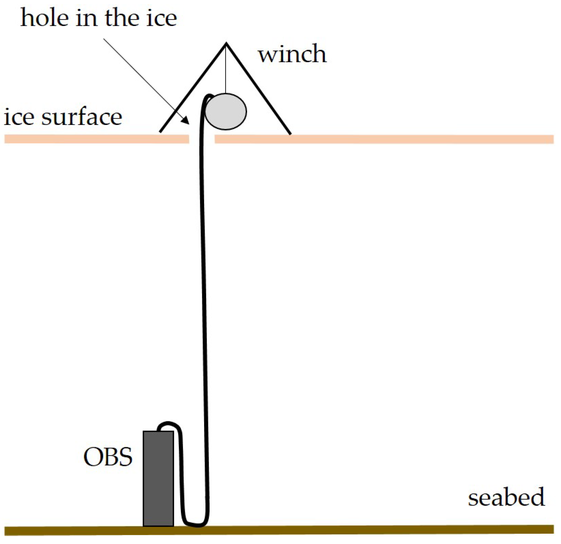
  • Various schemes for seismic stations’ deployment were described. It was concluded that the preferred schemes for deploying OBSs are those in which their subsequent dismantling does not depend on their power resources. Usually, such schemes provide for the possibility of dismantling stations via trawling and are suitable for shallow sea depths of up to 100 m. The advantages of such schemes include the possibility of installing additional hydrophysical and hydrobiological equipment, such as ADCP, CTD, thermistors, wave recorders, and biofouling plates.
  • The nuances of offshore work on the installation and recovery of equipment were outlined. It was concluded that particular attention should be paid to planning the recovery of seismic stations due to possible difficulties associated with the passage of a vessel to the deployment site due to unfavorable ice conditions. When deploying an OBS, it is advisable to choose the flattest seabed areas. Sandy soils are preferable to clay and silt soils because devices can become bogged down in them. Attention should be paid to avoiding increased galvanic corrosion in places where different metals are attached.
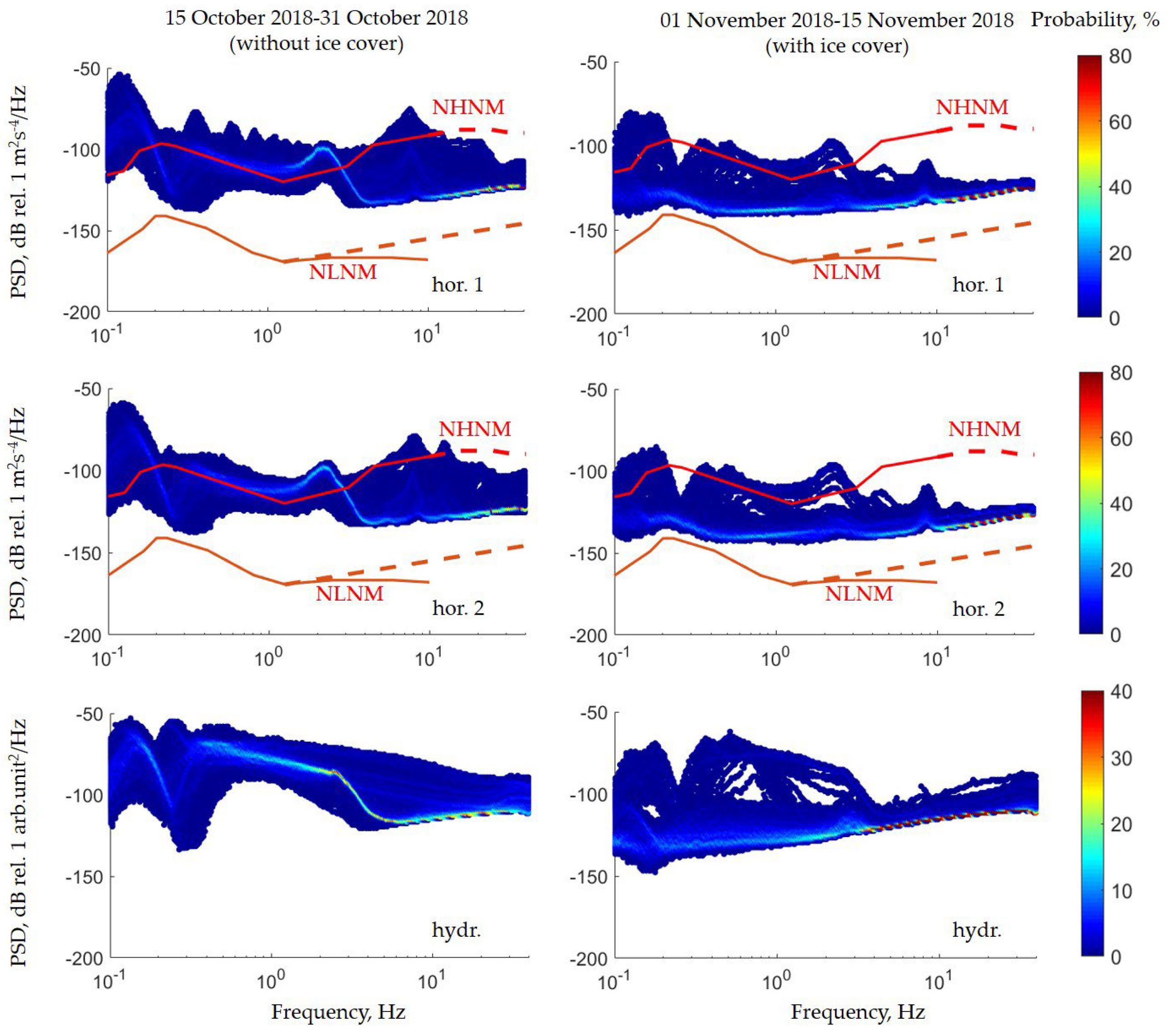
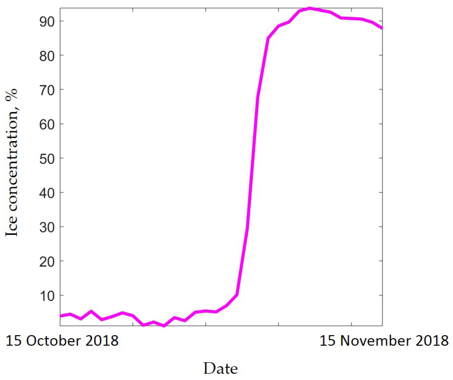
  • The features of seabed seismic records in the Arctic seas were demonstrated. It turned out that seabed seismic records are characterized by a high level of noise, especially during periods of time when there is no ice cover. Therefore, it is recommended to deploy OBSs for periods of time when ice cover is present. Seismic noise is caused by wind gravity waves, infragravity waves, and the coupling effect, and it also strongly depends on meteorological conditions, primarily on wind speed. The frequency range of the prevailing noise significantly overlaps with the frequency range of signals from both weak local earthquakes and strong distant ones. This must be taken into account when searching for and processing signals from earthquakes obtained in the Arctic seas.

Author Contributions

Conceptualization, A.A.K.; methodology, A.A.K.; validation, A.A.K.; formal analysis, A.A.K.; investigation, A.A.K., S.A.K., D.A.I., O.Y.G. and M.A.N.; resources, A.A.K., S.A.K., D.A.I., O.Y.G., V.N.I. and G.K.T.; data curation, A.A.K.; writing—original draft preparation, A.A.K.; writing—review and editing, all authors; visualization, A.A.K., M.A.N. and D.A.I.; supervision, A.A.K., L.I.L. and I.P.S.; project administration, A.A.K., I.P.S. and K.A.R.; funding acquisition, A.A.K., I.P.S., O.S.S. and K.A.R. All authors have read and agreed to the published version of the manuscript.

Funding

This work was financially supported by the following initiatives: the Russian Science Foundation, project no. 23-17-00125 (analysis and description of seismicity in the Laptev Sea region) and project no. 21-77-30001 (partially organizing expeditions to the Eastern Arctic Seas for the investigation of the permafrost state); the Ministry of Science and High Education of the Russian Federation, project “Priority-2030”, Tomsk State University (partially organizing expeditions to the Eastern Arctic Seas for the investigation of methane seepage); and the Russian State Assignment, project no. FMWE-2021-0011 (the design and description of a pop-up OBS and seismograph for installation on ice).

Institutional Review Board Statement

Not applicable.

Informed Consent Statement

Not applicable.

Data Availability Statement

Data are contained within the article.

Conflicts of Interest

The authors declare no conflict of interest.

References

  1. OBSIP Experiment Archive. Available online: https://obsic.whoi.edu/experiments/obsip-experiment-archive/ (accessed on 1 October 2023).
  2. Aderhold, K.; Woodward, R.; Frassetto, A. Ocean Bottom Seismograph Instrument Pool; Final Report; National Science Foundation: Alexandria, VA, USA, 2019; 80p. [Google Scholar]
  3. SAGE. Seismological Facility for the Advancement of Geoscience. Available online: http://ds.iris.edu/mda/_OBSIP/ (accessed on 1 October 2023).
  4. Cai, C.; Wiens, D.A.; Shen, W.; Eimer, M. Water input into the Mariana subduction zone estimated from ocean-bottom seismic data. Nature 2018, 563, 389–392. [Google Scholar] [CrossRef] [PubMed]
  5. Isse, T.; Kawakatsu, H.; Yoshizawa, K.; Takeo, A.; Shiobara, H.; Sugioka, H.; Ito, A.; Suetsugu, D.; Reymond, D. Surface wave tomography for the Pacific Ocean incorporating seafloor seismic observations and plate thermal evolution. Earth Planet. Sci. Lett. 2019, 510, 116–130. [Google Scholar] [CrossRef]
  6. Mark, H.F.; Lizarralde, D.; Collins, J.A.; Miller, N.C.; Hirth, G.; Gaherty, J.B.; Evans, R.L. Azimuthal seismic anisotropy of 70 Ma Pacific-plate upper mantle. J. Geophys. Res. Solid Earth 2019, 124, 1889–1909. [Google Scholar] [CrossRef]
  7. Corela, C.; Loureiro, A.; Duarte, J.L.; Matias, L.; Rebelo, T.; Bartolomeu, T. The effect of deep ocean currents on ocean- bottom seismometers records. Nat. Hazards Earth Syst. Sci. 2023, 23, 1433–1451. [Google Scholar] [CrossRef]
  8. Zali, Z.; Rein, T.; Krüger, F.; Ohrnberger, M.; Scherbaum, F. Ocean bottom seismometer (OBS) noise reduction from horizontal and vertical components using harmonic–percussive separation algorithms. Solid Earth 2023, 14, 181–195. [Google Scholar] [CrossRef]
  9. Liu, D.; Yang, T.; Wang, Y.; Wu, Y.; Huang, X. Pankun: A New Generation of Broadband Ocean Bottom Seismograph. Sensors 2023, 23, 4995. [Google Scholar] [CrossRef] [PubMed]
  10. Nakano, M.; Nakamura, T.; Kamiya, S.-I.; Kaneda, Y. Seismic activity beneath the Nankai trough revealed by DONET ocean-bottom observations. Mar. Geophys. Res. 2014, 35, 271–284. [Google Scholar] [CrossRef]
  11. Suzuki, K.; Nakano, M.; Takahashi, N.; Hori, T.; Kamiya, S.; Araki, E.; Nakata, R.; Kaneda, Y. Synchronous changes in the seismicity rate and ocean-bottom hydrostatic pressures along the Nankai trough: A possible slow slip event detected by the Dense Oceanfloor Network system for Earthquakes and Tsunamis (DONET). Tectonophysics 2016, 680, 90–98. [Google Scholar] [CrossRef]
  12. Barnes, C.R.; Best, M.M.R.; Zielinski, A. The NEPTUNE Canada Regional Cabled Ocean Observatory. Sea Technol. 2008, 49, 10–14. [Google Scholar]
  13. Barnes, C.R.; Best, M.M.R.; Johnson, F.R.; Pirenne, B. Final installation and initial operation of the world’s first regional cabled ocean observatory (NEPTUNE Canada). CMOS Bull. SCMO 2010, 38, 2–9. [Google Scholar]
  14. Lobkovsky, L.I.; Kuzin, I.P.; Kovachev, S.A.; Krylov, A.A. Seismicity of the Central Kuril Islands before and after the catastrophic M = 8.3 (November 15, 2006) and M = 8.1 (January 13, 2007) earthquakes. Dokl. Earth Sci. 2015, 464, 1101–1105. [Google Scholar] [CrossRef]
  15. Kuzin, I.P.; Kovachev, S.A.; Lobkovskii, L.I. Seismic microzonation and assessment of earthquake hazard for the construction sites of sea-based facilities in low seismicity water areas. J. Volcanol. Seism. 2009, 3, 131–143. [Google Scholar] [CrossRef]
  16. Simpson, D.W.; Leith, W. The 1976 and 1984 Gazli, USSR, earthquakes—Were they induced? Bull. Seismol. Soc. Am. 1985, 75, 1465–1468. [Google Scholar]
  17. Vlek, C. Induced Earthquakes from Long-Term Gas Extraction in Groningen, the Netherlands: Statistical Analysis and Prognosis for Acceptable-Risk Regulation. Risk Anal. 2018, 38, 1455–1473. [Google Scholar] [CrossRef]
  18. Kovachev, S.A.; Krylov, A.A. Results of Seismological Monitoring in the Baltic Sea and Western Part of the Kaliningrad Oblast Using Bottom Seismographs. Izv. Phys. Solid Earth 2023, 59, 190–208. [Google Scholar] [CrossRef]
  19. Piskarev, A.L. Arctic Basin: Geology and Morphology; VNIIOkeangeologiya: St. Petersburg, Russia, 2016; 291p. (in Russian) [Google Scholar]
  20. Krylov, A.A.; Ivashchenko, A.I.; Kovachev, S.A.; Tsukanov, N.V.; Kulikov, M.E.; Medvedev, I.P.; Ilinskiy, D.A.; Shakhova, N.E. The Seismotectonics and Seismicity of the Laptev Sea Region: The Current Situation and a First Experience in a Year-Long Installation of Ocean Bottom Seismometers on the Shelf. J. Volcanol. Seism. 2020, 14, 379–393. [Google Scholar] [CrossRef]
  21. Krylov, A.A.; Egorov, I.V.; Kovachev, S.A.; Ilinskiy, D.A.; Ganzha, O.Y.; Timashkevich, G.K.; Roginskiy, K.A.; Kulikov, M.E.; Novikov, M.A.; Ivanov, V.N.; et al. Ocean-Bottom Seismographs Based on Broadband MET Sensors: Architecture and Deployment Case Study in the Arctic. Sensors 2021, 21, 3979. [Google Scholar] [CrossRef]
  22. Krylov, A.A.; Kulikov, M.E.; Kovachev, S.A.; Medvedev, I.P.; Lobkovsky, L.I.; Semiletov, I.P. Peculiarities of the HVSR Method Application to Seismic Records Obtained by Ocean-Bottom Seismographs in the Arctic. Appl. Sci. 2022, 12, 9576. [Google Scholar] [CrossRef]
  23. Krylov, A.A.; Lobkovsky, L.I.; Rukavishnikova, D.D.; Baranov, B.V.; Kovachev, S.A.; Dozorova, K.A.; Tsukanov, N.V.; Semiletov, I.P. New Data on Seismotectonics of the Laptev Sea from Observations by Ocean Bottom Seismographs. Dokl. Earth Sci. 2022, 507, 936–940. [Google Scholar] [CrossRef]
  24. Krylov, A.A.; Ananiev, R.A.; Chernykh, D.V.; Alekseev, D.A.; Balikhin, E.I.; Dmitrevsky, N.N.; Novikov, M.A.; Radiuk, E.A.; Domaniuk, A.V.; Kovachev, S.A.; et al. A Complex of Marine Geophysical Methods for Studying Gas Emission Process on the Arctic Shelf. Sensors 2023, 23, 3872. [Google Scholar] [CrossRef]
  25. Webb, S.C. Broadband seismology and noise under the ocean. Rev. Geophys. 1998, 36, 105–142. [Google Scholar] [CrossRef]
  26. Janiszewski, H.A.; Eilon, Z.; Russell, J.B.; Brunsvik, B.; Gaherty, J.B.; Mosher, S.G.; Hawley, W.B.; Coats, S. Broad-band ocean bottom seismometer noise properties. Geophys. J. Int. 2023, 233, 297–315. [Google Scholar] [CrossRef]
  27. Schlindwein, V.; Müller, C.; Jokat, W. Seismoacoustic evidence for volcanic activity on the ultraslow spreading Gakkel Ridge, Arctic Ocean. Geophys. Res. Lett. 2005, 32, L18306. [Google Scholar] [CrossRef]
  28. Schlindwein, V.; Müller, C.; Jokat, W. Microseismicity of the ultraslow spreading Gakkel ridge, Arctic Ocean: A pilot study. Geophys. J. Int. 2007, 169, 100–112. [Google Scholar] [CrossRef]
  29. Schlindwein, V.; Schmid, F. Mid-ocean-ridge seismicity reveals extreme types of ocean lithosphere. Nature 2016, 535, 276–279. [Google Scholar] [CrossRef]
  30. Schlindwein, V.; Riedel, C. Location and source mechanism of sound signals at Gakkel ridge, Arctic Ocean: Submarine Strombolian activity in the 1999–2001 volcanic episode. Geochem. Geophys. Geosyst. 2010, 10, Q01002. [Google Scholar] [CrossRef]
  31. Koulakov, I.; Schlindwein, V.; Liu, M.; Gerya, T.; Jakovlev, A.; Ivanov, A. Low-degree mantle melting controls the deep seismicity and explosive volcanism of the Gakkel Ridge. Nat. Commun. 2022, 13, 3122. [Google Scholar] [CrossRef] [PubMed]
  32. R-Sensors. Seismic Instruments for Science and Engineering. Available online: https://r-sensors.ru/en/ (accessed on 1 October 2023).
  33. Logys. Available online: https://logsys.ru/ (accessed on 1 October 2023).
  34. Shakhova, N.; Semiletov, I.; Sergienko, V.; Lobkovsky, L.; Yusupov, V.; Salyuk, A.; Salomatin, A.; Chernykh, D.; Kosmach, D.; Panteleev, G.; et al. The East Siberian Arctic Shelf: Towards further assessment of permafrost-related methane fluxes and role of sea ice. Philos. Trans. R. Soc. A 2015, 373, 20140451. [Google Scholar] [CrossRef]
  35. Shakhova, N.; Semiletov, I.; Gustafsson, Ö.; Sergienko, V.; Lobkovsky, L.; Dudarev, O.; Tumskoy, V.; Grigoriev, M.; Mazurov, A.; Salyuk, A.; et al. Current rates and mechanisms of subsea permafrost degradation in the East Siberian Arctic Shelf. Nat. Commun. 2017, 8, 15872. [Google Scholar] [CrossRef]
  36. Shakhova, N.; Semiletov, I.; Chuvilin, E. Understanding the Permafrost–Hydrate System and Associated Methane Releases in the East Siberian Arctic Shelf. Geosciences 2019, 9, 251. [Google Scholar] [CrossRef]
  37. Kennett, B.L.N. Seismological Tables: ak135; Research School of Earth Sciences, The Australian National University: Canberra, Australia, 2005; 289p. [Google Scholar]
  38. Overduin, P.P.; Haberland, C.; Ryberg, T.; Kneier, F.; Jacobi, T.; Grigoriev, M.N.; Ohrnberger, M. Submarine permafrost depth from ambient seismic noise. Geophys. Res. Lett. 2015, 42, 7581–7588. [Google Scholar] [CrossRef]
  39. International Seismological Centre. Available online: http://www.isc.ac.uk/iscbulletin/search/ (accessed on 1 October 2023).
  40. U.S. Geological Survey. Available online: https://earthquake.usgs.gov/earthquakes/search/ (accessed on 1 October 2023).
  41. “Earthquakes of Russia” Database. Geophysical Survey of the Russian Academy of Sciences. Available online: http://eqru.gsras.ru/ (accessed on 1 October 2023).
  42. Chava, A.; Gebruk, A.; Kolbasova, G.; Krylov, A.; Tanurkov, A.; Gorbuskin, A.; Konovalova, O.; Migali, D.; Ermilova, E.; Shabalin, N.; et al. At the Interface of Marine Disciplines: Use of Autonomous Seafloor Equipment for Studies of Biofouling Below the Shallow-Water Zone. Oceanography 2021, 34, 61–70. [Google Scholar] [CrossRef]
  43. Ananyev, R.; Dmitrevskiy, N.; Jakobsson, M.; Lobkovsky, L.; Nikiforov, S.; Roslyakov, A.; Semiletov, I. Sea-ice ploughmarks in the eastern Laptev Sea, East Siberian Arctic shelf. Geol. Soc. Lond. Mem. 2016, 46, 301–302. [Google Scholar] [CrossRef]
  44. Nikiforov, S.L.; Ananiev, R.A.; Libina, N.V.; Dmitrevskiy, N.N.; Lobkovskii, L.I. Ice Gouging on Russia’s Arctic Shelf. Oceanology 2019, 59, 422–424. [Google Scholar] [CrossRef]
  45. Guidelines for the Implementation of the H/V Spectral Ration Technique on Ambient Vibrations Measurements, Processing and Interpretation; SESAME European research project WP12—Deliverable D23.12, European Commission—Research General Directorate Project No. EVG1-CT-2000-00026 SESAME; European Comission: Geneva, Switzerland, 2004; 62p.
  46. Kuznetsov, M.Y.; Shevtsov, V.I.; Poljanichko, V.I. Inderwater noise characteristics of TINRO-Center’s reseach vessels. Izv. TINRO 2014, 177, 235–256. (In Russian) [Google Scholar]
  47. Pisarev, S.V. Modern drifting robotic devices for contact measurements of the physical characteristics of the Arctic basin. Oceanol. Res. 2019, 47, 5–31. (In Russian) [Google Scholar] [CrossRef]
  48. OSI SAF Global Sea Ice Concentration Climate Data Record v2.0—Multimission, EUMETSAT SAF on Ocean and Sea Ice, 2017. Available online: https://navigator.eumetsat.int/product/EO:EUM:DAT:MULT:OSI-450 (accessed on 1 October 2023).
  49. Peterson, J. Observation and Modeling of Seismic Background Noise; U.S. Geological Survey Open-File Report; US Geological Survey: Reston, VA, USA, 1993; pp. 93–322. [Google Scholar]
  50. Wolin, E.; McNamara, D.E. Establishing High-Frequency Noise Baselines to 100 Hz Based on Millions of Power Spectra from IRIS MUSTANG. Bull. Seism. Soc. Am. 2020, 110, 270–278. [Google Scholar] [CrossRef]
  51. Longuet-Higgins, M.S. A theory for the generation of microseisms. Philos. Trans. R. Soc. A 1950, 243, 1–35. [Google Scholar]
  52. Lepore, S.; Grad, M. Analysis of the primary and secondary microseisms in the wavefield of the ambient noise recorded in northern Poland. Acta Geophys. 2018, 66, 915–929. [Google Scholar] [CrossRef]
  53. Hersbach, H.; de Rosnay, P.; Bell, B.; Schepers, D.; Simmons, A.J.; Soci, C.; Abdalla, S.; Balmaseda, M.A.; Balsamo, G.; Bechtold, P.; et al. Operational Global Reanalysis: Progress, Future Directions and Synergies with NWP; ERA Report Series no. 27; European Centre for Medium Range Weather Forecasts: Reading, UK, 2018. [Google Scholar]
Figure 1. (a) Design of the MPSSR ocean-bottom seismographs: 1—three-component broadband MET seismometer CME-4311 [32], 2—three-component short-period electrodynamic seismometer (SV-10 and SG-10) placed in gimbal, 3—hydrophone 5007 m, 4—seismic recorder URS-S, 5—digital compass module, 6—battery pack, 7—protective half-cover for hydrophone, 8—duralumin sphere, 9—concrete ballast. (b) External view of the MPSSR. (c) Design of the Typhoon ocean-bottom seismographs: 1—three-component short-period MET seismometer CME-3311 [32], 2—hydrophone 5007 m, 3—seismic recorder URS-S, 4—battery pack, 5—protective half-cover for the hydrophone, 6—duralumin sphere, 7—concrete ballast. (d) External view of the Typhoon.
Jmse 11 02221 g001
Figure 2. (a) Design of the GNS and GNS-C ocean-bottom seismographs: 1—three-component geophone SM-6 for GNS or MET seismometer CME-4111 [32] for GNS-C, 2—seismic recorder GNS, 3—acoustic modem, 4—battery (or accumulator) pack, 5—acoustic hydrophone, 6—seismic hydrophone (HTI-94-SSQ for GNS or EDBOE RAS for GNS-C), 7—glass spherical housing, 8—ballast, 9—lamp, 10—flag, 11—anchor release, 12—plastic case. (b) External view of the GNS. (c) External view of the GNS-C.
Jmse 11 02221 g002
Figure 3. (a) Design of OBS for installation through holes in ice: 1—seismic recorder URS-S, 2—three-component short-period MET seismometer CME-3311 [32], 3—battery pack, 4—plastic housing, 5—fastening pins, 6—eyes for fastening a rope or cable, 7—ballast. (b) View of the internal layout of the OBS. (c) External view of the OBS.
Jmse 11 02221 g003
Figure 4. (a) Design of seismic stations for installation on ice: 1—seismic recorder DELTA-03M [33], 2—three-component electrodynamic seismometer SPV-3K [33], 3—block of additional sensors (inclinometer, thermometer, electronic compass, and battery voltage indicator), 4—hydrophone 5007 m, 5—metal housing. (b) View of the internal layout of the station. (c) External view of station with the hydrophone on a cable.
Jmse 11 02221 g004
Figure 5. Location of OBS deployments in the Russian Arctic: (a) in the Barents and Kara seas, and (b) in the Laptev Sea and the East Siberian Sea. Long-term deployments (3–7 months)—red circles, short-term deployments (1 h–15 days)—blue circles.
Jmse 11 02221 g005
Figure 9. Deployment schemes used for non-pop-up OBSs on the shelf to depths of 100 m: (a) using submerged buoys and an external acoustic release, (b) without using submerged buoys and an external acoustic release, and (c) using additional measuring devices.
Jmse 11 02221 g009
Figure 10. The workflow of deploying non-pop-up OBSs on the shelf to depths of 100 m: (a) lowering the station to the seafloor, (b) laying out a rope on the seafloor in a drift, and (c) dropping the ballast.
Jmse 11 02221 g010
Figure 11. The workflow for dismantling non-pop-up OBSs on the shelf using the trawling method.
Jmse 11 02221 g011
Figure 12. The workflow for deploying (ac) and dismantling (df) pop-up OBSs.
Jmse 11 02221 g012
Figure 13. A scheme for the short-term installation of non-pop-up OBSs on the shelf in order to measure seafloor seismic noise using the HVSR method.
Jmse 11 02221 g013
Figure 14. A scheme of the short-term installation of OBSs on the shelf through holes in the ice.
Jmse 11 02221 g014
Figure 15. A scheme for deploying a seismograph on ice.
Jmse 11 02221 g015
Figure 16. Seismic noise PSD curves recorded on the Laptev Sea shelf during the periods of 15 October 2018–31 October 2018 (left) and 1 November 2018–15 November 2018 (right). The solid red lines indicate the curves of the NHNM (new high-noise model) and NLNM (new low-noise model) [49], while the red dotted lines indicate the extension of the NHNM and NLNM according to [50]. The color indicates the probability of finding the noise curve in a certain area of the graph.
Jmse 11 02221 g016
Figure 17. Ice concentration curve according to EUMETSAT reanalysis (mesh size: 25 km) [48] for the period of 15 October 2018–15 November 2018 for the closest node to the location of the OBS that corresponded to the PSD curves shown in Figure 16.
Jmse 11 02221 g017
Figure 18. Time dependence of wind speed for the location of the OBS in the Laptev Sea obtained as a result of the ERA5 reanalysis [53] and its correlation with the seafloor seismic noise level at the same point shown in the spectrogram—two record fragments (a,b).
Jmse 11 02221 g018
Table 1. Main parameters of seismic stations for use in Arctic seas.
TypeMPSSRTyphoonGNSGNS-COBS for Installation through Ice HolesSeismograph for Installation on Ice
DeveloperIO RASIO RASIP Ilinsky D.A.IO RAS/IP Ilinsky D.A.IO RASIO RAS
Dimensions44 cm (diam.)37 cm (diam.) 33 cm (diam.)43 cm (diam.) 21 × 21 × 68 cm276 cm (diam.)
75 cm (height)
Maximum depth
(housing)
3000 m2000 m6000 m6000 m30 m
SensorsThree-component seismometer CME-4311, three-component geophone SH/SV-10, hydrophone 5007 mThree-component seismometer CME-3311, hydrophone 5007 mThree-component seismometer SM-6,
hydrophone HTI-94-SSQ
Three-component seismometer CME-4111/4311, hydrophone EDBOE RASThree-component seismometer CME-3311Three-component seismometer SPV-3K,
hydrophone 5007 m
Number of channels744434/8
Frequency band0.0167–50 Hz
(CME-4311),
10–250 Hz
(SH/SV-10),
0.04–2500 Hz
(5007 m)
1–50 Hz
(CME-3311),
0.04–2500 Hz
(5007 m)
4.5–140 Hz
(SM-6),
2–30,000 Hz
(HTI-94-SSQ)
0.0083–50 Hz
(CME-4111),
0.067–30,000 Hz
(EDBOE RAS)
1–50 Hz
(CME-3311)
0.5–65 Hz
(SPV-3K),
0.04–2500 Hz
(5007 m)
Sensitivity2000 V/m/s
(CME-4311),
28 V/m/s
(SH/SV-10),
7.2 ± 0.5 mV/Pa
(5007 m)
2000 V/m/s
(CME-3311),
7.2 ± 0.5 mV/Pa
(5007 m)
28.8 V/m/s
(SM-6),
12.6 V/Bar (HTI-94-SSQ without preamp)
4000 V/m/s
(CME-4111/4311),
200 V/bar
(EDBOE RAS)
2000 V/m/s
(CME-3311)
500 V/m/s
(SPV-3K)
Dynamic range122 dB
(CME-4311),
100 dB (5007 m)
118 dB
(CME-3311),
100 dB (5007 m)
140 dB
(SM-6),
198 dB
(HTI-94-SSQ without preamp)
122 dB
(CME-4111),
120 dB
(EDBOE RAS)
118 dB
(CME-3311)
120 dB
(SPV-3K),
100 dB (5007 m)
Sample rates, Hz20, 25, 40, 50, 80, 100, 160, 200, 400, 80020, 25, 40, 50, 80, 100, 160, 200, 400, 80062.5, 125, 250, 500, 1000, 2000, 400062.5, 125, 250, 500, 1000, 2000, 400020, 25, 40, 50, 80, 100, 160, 200, 400, 80031.25, 62.5, 125, 250, 500, 1000
Time synchronizationGPS GPS GPS
GLONASS
GPS
GLONASS
GPS GPS
Temperature stability of the quartz generator±5 × 10⁻⁹±5 × 10⁻⁹±5 × 10⁻⁹±5 × 10⁻⁹±5 × 10−910−7 (basic)
10−8 (optional)
MemorySD card up to 64 GbSD card up to 64 GbSD card up to 128 GbSD card up to 128 GbSD card up to 64 GbSD card, 32 Gb
Allowed installation tilt angle±15°±15°±20°±15°±15°±15°
Temperature range
(sensors)
−12...+55 °C
(basic),
−40...+55 °C
(optional)
−12...+55 °C
(basic),
−40...+55 °C
(optional)
−40...+100 °C−12...+55 °C
(basic),
−40...+55 °C
(optional)
−12...+55 °C
(basic),
−40...+55 °C
(optional)
−30…+55 °C
Table 2. Locations, types of OBSs, and their operation periods in the Arctic seas.
TypeLatitude, ° NLongitude, ° EDepth, mWater AreaOperation Period
Long-term deployments
MPSSR75.42127.3942Laptev SeaOctober 2018–February 2019
MPSSR75.43129.1340Laptev SeaOctober 2018–March 2019
GNS-C77.31120.61350Laptev SeaOctober 2018–May 2019
MPSSR69.6755.1839Barents SeaAug 2018–November 2019
MPSSR69.4055.2629Barents SeaAug 2018–November 2019
MPSSR69.4856.0129Barents SeaAug 2018–November 2019
MPSSR69.7555.9344Barents SeaAug 2018–November 2019
MPSSR76.39125.6651Laptev SeaOctober 2019–January 2020
Typhoon76.83127.6961Laptev SeaOctober 2019–February 2020
Typhoon71.5466.4746Kara SeaOctober 2021–January 2022
Typhoon71.2465.6042Kara SeaOctober 2021–March 2022
Typhoon69.9765.3041Kara SeaOctober 2021–February 2022
MPSSR74.9069.7242Kara SeaOctober 2021–March 2022
Short-term deployments
GNS-C75.42129.1340Laptev Sea30 September 2018–6 October 2018
GNS-C76.86125.5775Laptev Sea28 September 2018–13 October 2018
MPSSR75.01126.5237Laptev Sea6 October 2018–9 October 2018
MPSSR75.01128.2636Laptev Sea5 October 2018–12 October 2018
MPSSR75.20127.4040Laptev Sea6 October 2018–8 October 2018
MPSSR74.94160.5245East Siberian Sea30 September 2019–3 October 2019
Typhoon72.9865.8782Kara Sea4 November 2022 (~1 h)
Typhoon69.1358.4217Barents Sea10 November 2022 (~1 h)
Typhoon69.2058.0321Barents Sea10 November 2022 (~1 h)
Typhoon69.2257.8122Barents Sea11 November 2022 (~1 h)
Typhoon69.3257.8222Barents Sea11 November 2022 (~1 h)
Disclaimer/Publisher’s Note: The statements, opinions and data contained in all publications are solely those of the individual author(s) and contributor(s) and not of MDPI and/or the editor(s). MDPI and/or the editor(s) disclaim responsibility for any injury to people or property resulting from any ideas, methods, instructions or products referred to in the content.

