Article

Morphological Response of a Highly Engineered Estuary to Altering Channel Depth and Restoring Wetlands

by
Rutger W. A. Siemes
1,*,
Trang Minh Duong
1,2,3,
Pim W. J. M. Willemsen
1,4,
Bas W. Borsje
1 and
Suzanne J. M. H. Hulscher
1
1
Department of Water Engineering and Management, University of Twente, 7500 Enschede, AE, The Netherlands
2
Department of Coastal and Urban Risk & Resilience, IHE Delft Institute for Water Education, 2611 Delft, AX, The Netherlands
3
Department of Harbour, Coastal and Offshore Engineering, Deltares, 2600 Delft, MH, The Netherlands
4
Department of Ecosystems and Sediment Dynamics, Deltares, 2600 Delft, MH, The Netherlands
*
Author to whom correspondence should be addressed.
J. Mar. Sci. Eng. 2023, 11(11), 2150; https://doi.org/10.3390/jmse11112150
Submission received: 13 October 2023 / Accepted: 8 November 2023 / Published: 11 November 2023

Abstract

:
Estuaries are continuously adapting to anthropogenic pressure. Because of sea-level rise and reduced fluvial sediment supply, they are at risk of sediment starvation. Contrarily, some estuaries require frequent dredging after artificially deepening the channel to maintain port operations. To optimize current estuarine functions and make estuaries more resilient to future threats, improved understanding of estuarine development after system changes is essential. This paper investigates the estuarine response related to two large-scale human interventions: (1) altering channel depth, following global trends of channel deepening for port navigability; and (2) creating or restoring wetlands, a nature-based solution increasingly explored for its ecosystem services. A schematized 2D-morphological model is set up using Delft3D-FM reflecting a highly engineered estuary in a micro-tidal and wave-dominant environment. Results demonstrate how channel deepening (from 13 m to 17 m, without wetland presence) increased sedimentation in the channel by +31%. Sedimentation rates in the wetland were mostly unaffected by channel depth. After restoring the wetland area (wetland width from 0 km to 1 km, constant channel depth of 15 m), sedimentation within the channel was reduced by 72 %. The wetland area not only served as sediment sink, but also increased the tidal flow, diminishing sedimentation throughout the estuarine channel. Further analysis showed that restoring wetland areas along a specific segment mostly affected channel sedimentation locally (i.e., at the channel segment along the restored wetland). As such, to alleviate dredging operations at critical locations in the navigation channel, strategic restoration of wetlands can be considered which can provide a sustainable alternative to dredging within highly engineered estuaries.

1. Introduction

Estuaries are constantly adjusting to anthropogenic stresses. When sea levels rise, and sediment supply by the rivers reduces, estuaries are at risk of sediment starvation and drowning of estuaries [1]. Furthermore, many estuaries undergo artificial deepening to enhance port operations, leading to natural sedimentation of the channels. This surplus sediment is frequently dredged to maintain navigability for ships and these dredging operations can result in a negative sediment budget in estuaries. Consequently, estuaries may drown due to dredging, which for many European estuaries is more likely than drowning due to sea-level rise [2]. In turn, drowning of estuaries can cause many problems, including increased problems with salinity intrusion [3], heightened flood risk by amplifying tides [4] and causing the loss highly valuable wetland ecosystems can drown [5].
Dredging and deepening the navigational channel upsets the balance between the deep channels and shallow intertidal areas which can promote sedimentation of tidal creeks and stabilization of the tidal flats [6,7]. In addition, estuaries are often channelized and embanked to stabilize the banks and to ensure flood safety and the intertidal wetlands are claimed, e.g., for agricultural use. Although these traditional engineering measures have proven effective for their intended purposes, they have frequently overlooked or produced adverse effects on estuarine morphology [8,9] and ecology (e.g., [10,11]). Typically, an estuary becomes artificially narrow and deep, with examples found worldwide, e.g., the Rhine–Meuse Delta, the Netherlands [12] or the Yangtze estuary, China [13] or many estuaries in the UK [14]. In such systems, the impact of engineering works on system functions often outweigh climate change impacts [2,3,15].
Recent research explores the restoration of wetlands (sometimes called managed realignment) such as salt marshes, a nature-based solution increasingly recognized for aiding in flood safety, for their potential to trap sediment [16] and hence their ability to keep up—within limits—with a rising sea level [17] and various other ecosystem services [18]. To this end, Ref. [19] states that science-based management practices could facilitate the restoration of intertidal wetlands, even under climate change impacts. However, such measures also come with downsides, as they require space as well as time to develop, and their complex interactions bring about uncertainties [20]. As such, to further improve understanding on wetland restoration projects and their impact on the entire system, recent research highlights the importance of studying basin-wide morphodynamics and using metrics such as sediment budgets to understand the distribution of sediments through the whole estuarine system and onto the intertidal wetland [21,22].
The impact of such engineering practices on estuarine morphology can be assessed a-priori using morphodynamic models. In tide-dominated estuaries, such models have successfully hind-casted decades to centuries of morphological development (e.g., [23,24,25]). However, morphological modeling within more complex estuarine environments in which not only tides but also seasonally varying waves and river discharge play a significant role on estuarine morphology, has to date proved cumbersome. As such, such modeling efforts have been limited to the timescale of several years [26,27]. Moreover, long-term morphological models are restricted in estuaries under constant artificial changes, e.g., constant dredging to maintain or increase channel depth. In such estuarine systems, short-term morphological models (timescale of months to years) can prove to be useful tools to simulate morphological development and to explore the impact of system changes on estuarine development.
In this study, we aim to explore and quantify the short-term (1 year) morphological response of engineered estuaries after two large-scale human interventions: (1) Changing the depth of the estuarine channel, representing a traditional engineering solution used globally to advance port operations and (2) Wetland restoration or creation, a nature-based solution increasingly recognized for numerous aforementioned ecosystem services. Hereto, we focus on answering the following questions: (1) How does channel deepening affect morphology in the coupled channel-wetland system and (2) To what extent can wetland restoration steer estuarine-wide morphology. To this end, a depth-averaged (2DH) process-based morphological model is developed with model assumptions reflecting a typical highly engineered estuary in a micro-tidal and wave-dominant environment.

2. Methods

2.1. Modeling Rationale

A morphological modeling framework is set up to assess the impact of two control variables in a highly engineered estuary: Channel depth and wetland area. Various modeling choices were made, which are rationalized below.

2.1.1. Time and Spatial Scale

Due to the difficulties with long-term (decadal+) morphological modeling addressed in the introduction, this paper utilizes short-term (1-year) morphological simulations (similar to [28,29]). The scope of this paper is to study the impact of human interventions in engineered estuaries, i.e., systems not in their morphodynamic equilibrium. Such estuaries are also often subject to frequent dredging to maintain channel depth for port navigability; hence these systems will not reach a ‘natural’ morphodynamic equilibrium as long as dredging activities continues. As such, the 1-year morphological simulations are intended to give insights into the initial response of the system after implementation of an intervention. The approach will not give insights into the equilibrium state or the time to reach this equilibrium.
Second, a difference in spatial scale exists when trying to accurately represent individual wetlands (<10 km 2 ) and the entire estuary (>100 km 2 ). Suitable to the research questions, the model is developed on the spatial scale of an entire estuary. This allows for the inclusion of all estuarine processes and how they vary throughout the domain. In this way, both fluvial- and ocean processes can be included.

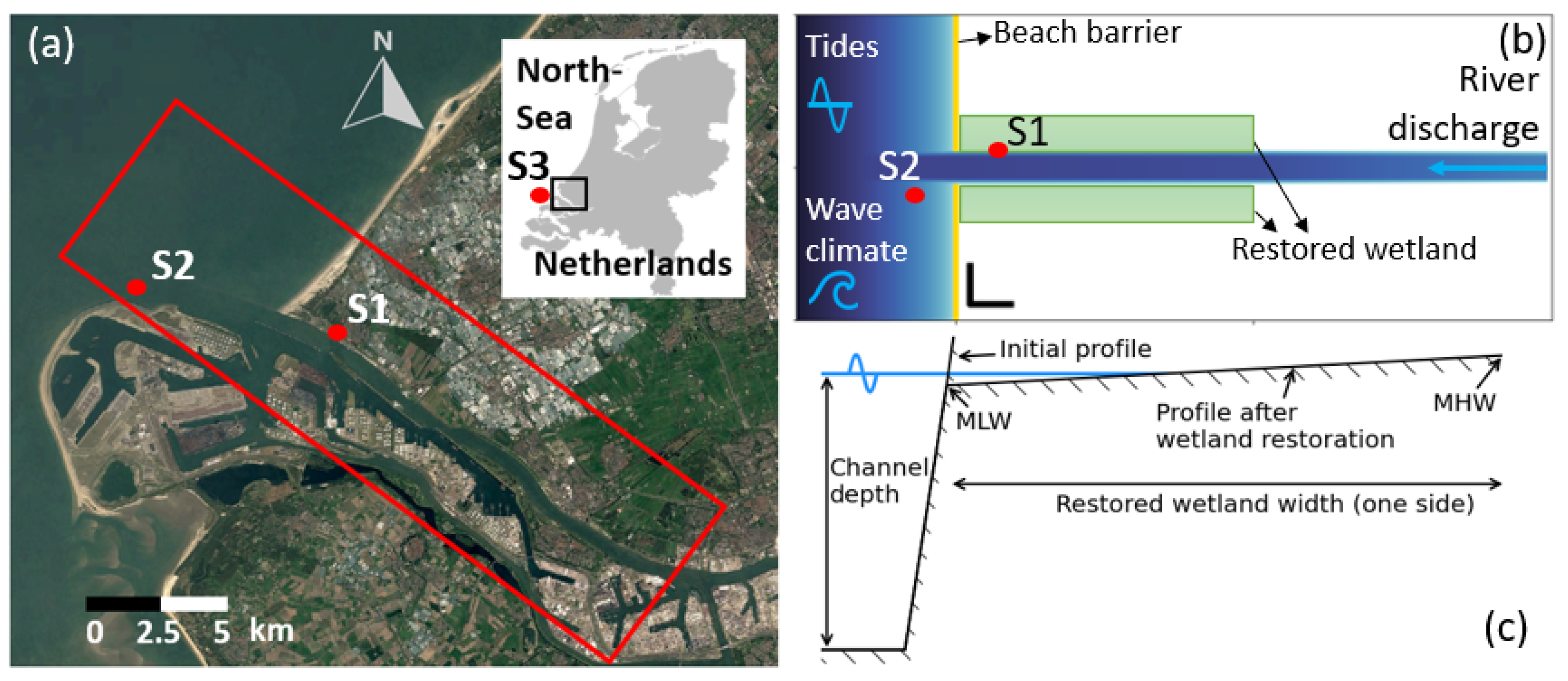
2.1.2. Schematized Domain

A schematized or simplified proxy of a highly engineered estuary is used. Such schematizations limit predictive power for the represented estuary, but they can help gain process-based system understanding by excluding physical components of the real system not relevant to the analysis. Consequently, schematized domains are commonly applied in the literature to gain qualitative insights into real estuarine development (e.g., see [28,30]).
The schematized domain is based on a study area (addressed below), which allows for model comparison and increases confidence in modeled results. However, only geometric features that are key for the research questions are included. As such, the domain is simplified to a straight estuarine channel with realistic channel depth and width but excluding local variations herein and a simplified coastal profile that is uniform in the along-shore direction.

2.1.3. Study Area

Modeling assumptions are based on the Rotterdam Waterway, an estuary located within the Rhine–Meuse Delta, the Netherlands. The estuary discharges the water from both the Rhine and Meuse catchment. Both rivers have relatively high discharges in winter and low discharges during summer, with a mean discharge of 1760 m 3 s 1 . The coastal zone has a mean tidal range of 1.65 m [31] and a typical average wave heights of 1.1 m [32]. This classifies the system in its natural state as a micro-tidal estuary where the wave-forcing is dominant over the tidal-forcing [33,34]. Such systems typically have sandy barriers around the mouth and a wider back-barrier basin with intertidal wetlands [33].
Due to extensive human interventions in the estuary, its present-day plan form is a straight and embanked channel which is frequently dredged to maintain its artificial depth, allowing large ships to enter the ports (Figure 1). Also, while historical records indicate that intertidal areas were abundantly present throughout the region [35,36,37], as a consequence of human interventions, presently there are little to no wetlands left in the estuary [12]. As such, its present-day layout is one of a highly engineered estuary.

2.2. Model Setup

2.2.1. Model Description

A schematized 2DH (depth-averaged) morphodynamic model is constructed using the Delft3D Flexible mesh software (DFM; version 2023.01), the successor to Delft3D which is extensively applied for morphodynamic modeling in estuarine environments (e.g., [25,29,30]). From DFM, the modules that solve flow (D-Flow), waves (D-Waves) and morphology (D-Morphology) are applied. The D-Flow module solves the unsteady shallow water equations in 2DH (depth-averaged; described in Appendix A), resulting in water levels and velocity fields over the model domain. D-Waves is a module which simulates propagation of waves, wave breaking, diffraction, refraction, and frequency shifting and generation by wind in coastal regions, using the third generation Simulating WAves Nearshore (SWAN) spectral wave model (based on [38]; Appendix A). The influence of vegetation on hydrodynamics was included by changing the local bed roughness, in D-Flow following the equations by [39], and in D-Waves by an increased drag coefficient. Based on the hydrodynamic characteristics, transport of sediments and exchange of sediments with the bed is calculated in the D-Morphology module. For cohesive sediments, transport is calculated using the advection-diffusion equations and exchange of cohesive sediments with the bed is determined using the Partheniades–Krone equations [40]. Non-cohesive sediment transport is solved using the equations of [41]. For more explanation on the governing processes and equations, see Appendix A. Extensive documentation of the software is available in the module’s respective manuals: [42,43,44].

2.2.2. Schematized Bathymetry

The schematized bathymetry reflects a highly engineered estuary in a micro-tidal, wave-dominant environment and is based on characteristics of the Rotterdam Waterway in the Rhine–Meuse Delta, the Netherlands. The domain consists of a coastal region and an estuarine region. The coastal zone extends 8 km seawards from the coastal boundary, up to 20 m below mean sea level, following Dean’s equilibrium profile ([45]; fitted using local bathymetry data by [46]). The area below 20 m was excluded, as the literature indicates that there is almost no net annual transport in this region [32]. The estuarine region extends 15 km landwards, ending before a confluence point upstream, and is the main area of interest. Following local bathymetry data, the channel is 15 m deep at the inlet and is 450 m wide, including 100 m wide banks. The channel slopes landwards with 5 × 10 5 m/m. The estuarine channel cuts through the coastal profile, maintaining its shape (Figure 1).
The grid of the flow-domain has a grid resolution of 50 × 25 m (50 m in the flow direction). Outside of the estuarine region, grid resolution gradually decreases in the flow direction towards 300 m at the outer edges. This way, the resolution at the inlet and in the surf zone was kept high. For the wave module, two nested domains were applied, whereby the inner wave domain mimics the flow domain. The outer wave domain expands in the long-shore direction of the coastal area to prevent wave shadowing and has grid sizes increased by a factor of 4. For a full overview of applied model parameters, see Table 1.

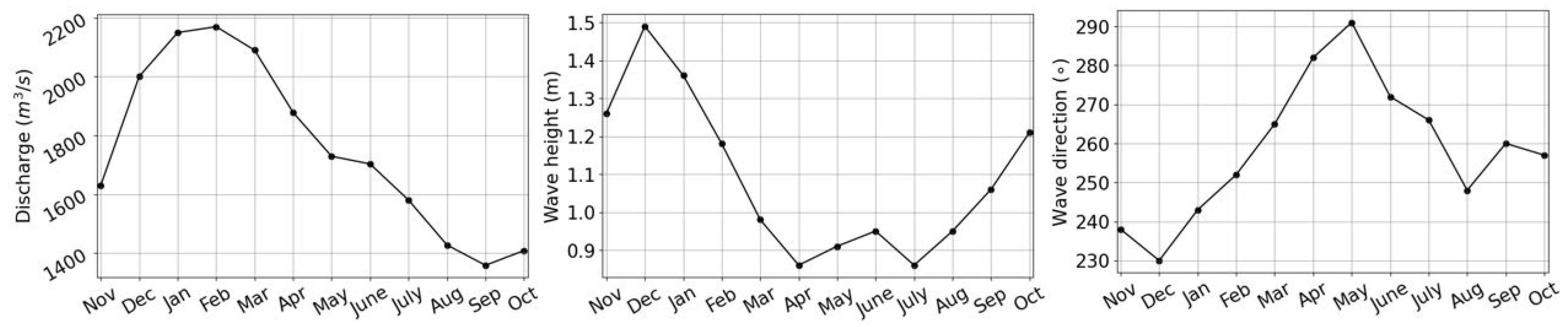
2.2.3. Model Forcing

The domain was forced by tides and waves from the offshore boundary and by a fluvial (sediment) discharge at the river boundary. Values used are inspired by the Rotterdam Waterway estuary. Tides consisted of an M2 component with an amplitude of 0.8 m, an M4 component of 0.17 m with a 6 phase difference, an M6 component with a 234 phase difference and an S2 component with an amplitude of 0.15 m [31,49]. The S2 phase was slightly adjusted such that the spring-neap cycle repeats exactly every 14 days.
Considering the stochastic nature of the system’s climate, monthly averaged wave climate and river discharges were derived. Subsequently, these monthly averages were compressed into 14 days to fit the 14-day tidal spring-neap cycle. By using an acceleration factor (AF) of 26, one spring-neap cycle of hydrodynamics results in 1 year of morphological development. Both the wave and discharge climate are compressed to fit within the 14-day tidal cycle. Monthly average wave characteristics were derived based on wave data between 2010 and 2020 at the nearest offshore measurement station Lichteiland Goeree; (S3 in Figure 1; [50]). An average wave height of 1.1 m was identified, similar to [32], which fluctuated between 0.85 m in summer and 1.5 m in winter; the mean wave direction was 260°, fluctuating between 230° and 290° in winter and summer, respectively (Figure 2).
A representative discharge regime was derived based on observed discharges into the RMD system between 2010 and 2020 (observed by the national water authority; [50]) and representative discharge curves derived for the Rhine and Meuse entering the Netherlands [51], at Lobith and Borgharen. It is assumed that 89% of the total Rhine and Meuse’s water discharges into the North Sea via the Rotterdam Waterway and the Haringvliet estuary. The Haringvliet estuary discharges a part of this water during periods of medium to high river discharge. The Haringvliet gates are presumed to operate such that they discharge 40% of the monthly average discharge above a threshold discharge of 1000 m 3 / s . This results in an annual average discharge of the Rotterdam Waterway of 1760 m 3 / s , which fluctuates between ∼1400 m 3 and ∼2150 m 3 in summer and winter, respectively (Figure 2). Upstream suspended sediment concentrations (SSC) were set such that SSC into the estuarine region fit observations by regional and national authorities [50,52], resulting in an upstream SSC set to 30 mg/L. Assuming an equilibrium sediment profile at the coastal boundaries, sediment concentrations here were set equal to their equilibrium concentrations.

2.2.4. Morphological Settings

The bed of the Rotterdam Waterway and surroundings consist of relatively coarse sand, with a median grain size ( D 50 ) of ∼200 μ m [47]. A mixture of cohesive and non-cohesive sediments coming from the river and coast settles in the channel, but these sediments are constantly dredged to maintain channel depth. To represent the system after dredging has occurred, an initial bed of sand with a D 50 of 200 μ m was deemed appropriate. At the upstream river boundary, fluvial sediment is supplied consisting of cohesive sediment, representing mud with a typical dry bed density of 500 kg/ m 3 and sediment settling velocity of 0.25 mm/s.

2.2.5. Vegetation

A vegetation cover is added in the created wetlands, which is static over the 1-year simulation. The vegetation cover was predicted using an empirical relationship derived in [53], which is based on a database of a combined literature and GIS study of 60+ marshes worldwide. These salt marshes had a wide range of local mean tidal range (MTR) (between 0.5 and 10 m) and observed salt marsh vegetation species with either Spartina anglica or Salicornia. The formulation relates the lowest observed elevation for marsh vegetation with locally observed tidal datums in front of the marsh, as follows:
P i o h = 108.23   cm l o g 10 ( M T R ) + 163.21   cm
wherein P i o h (cm) is the minimum bed-elevation on which vegetation can grow relative to mean high water (MHW; in cm), MTR is the mean tidal range (cm).
When applying this equation directly in the numerical model, a cell with a bed-elevation equal to P i o h will be fully vegetated ( F v e g = 1). However, in reality, roughly half of that cell’s bed-elevation would be below the vegetation threshold P i o h (assuming linear slopes between cells). To overcome this, a normal cumulative density function (CDF) was applied around P i o h . This way, the grid cell with a bed-elevation equal to P i o h (which is the average bed-elevation of that cell) has a F v e g of 0.5. The mean and standard deviation used in the CDF are derived directly from the dataset obtained by [53]. Values outside the 95% confidence interval were rounded off.
The drag that vegetation exerts on the flow is derived using the [39] equations (Appendix A. Following [48], a fully vegetated marsh area ( F v e g = 1 ) has a vegetation density of 1200 stems/ m 2 , with a uniform stem diameter of 4.3 mm and stem height of 0.5 m. For the impact of vegetation on waves, a constant wave drag coefficient ( C D ) of 0.7 was applied. This was chosen following previous work by [54], as it represents vegetation drag during average wave conditions [55,56]). Table 1 gives an overview of all vegetation parameters.

2.3. Large-Scale Interventions

The model scenarios were systematically varied with different combinations of (1) channel depth, (2) landward extent of the wetland, and (3) location and width of the wetland zone (Table 2). A visual representation of these interventions is given in Figure 1.
Scenarios for changing channel depth represent the global trend to deepen estuaries for port navigability. The channel depth is varied around the system’s depth in recent history, between 13–17 m. Changing wetland area’s (scenarios #2 and #3) represent either claiming or restoring/creating wetlands. Traditionally, wetlands are often claimed for human use (e.g., agriculture). Presently, restoration of wetlands is also increasingly common as a nature-based solution for their numerous ecosystem services. Wetlands are restored along both banks for up to 1 km in total width (0.5 km per side). Their elevation starts at mean low water (MLW) along to the channel and increases linearly to mean high water (MHW). The intertidal wetland and the coast are separated by a 100 m wide sandy barrier (Figure 1), typical for wave-dominant estuaries [33].

2.4. Model Output Analysis

For analysis of the morphological model results, the focus is on the estuarine region of the domain, between 0–15 km inland from the estuarine mouth. Morphological results are averaged in the cross-channel direction (x-direction in Figure 1) or the cross-section (y-direction in Figure 1) or averaged over an entire section. Morphological development is reported in accretion or erosion rates (m) or in terms of the area’s annual sediment budget. For the latter, the sediment’s bulk density is used (Mton, or 10 kg), relevant for dredging practices.
Also, the estuary’s spring ebb tidal prism (P) and the inlet’s cross-sectional area (A) are used for the analysis of the results. To predict if estuarine inlets are likely to erode or accrete or if the inlet size is close its their equilibrium, P/A equilibrium relationships are often used (e.g., [28,57,58]). In this work, P and A are analyzed and compared to the sediment budget of the estuary.
P is derived by computing the maximum volume of water through the inlet, excluding the river discharge, over the spring-neap cycle to obtain the spring tidal prism. Subsequently, the annual average discharge is added to obtain the spring ebb tidal prism. A is derived by computing the initial cross-sectional area along the inlet, from the coastal boundary up to 100 m landwards.

3. Results

3.1. Reference Scenario

First, results with the reference layout are reported; the model configuration that most closely reflects the study area in recent history (around 2010, as channel deepening has occurred afterwards). The channel depth is 15 m, and the wetland width is 0 km, as visualized in Figure 1 and indicated in Table 2 above. Modeled results are compared to observations to indicate they are in a realistic order of magnitude and improve confidence in the model’s performance.

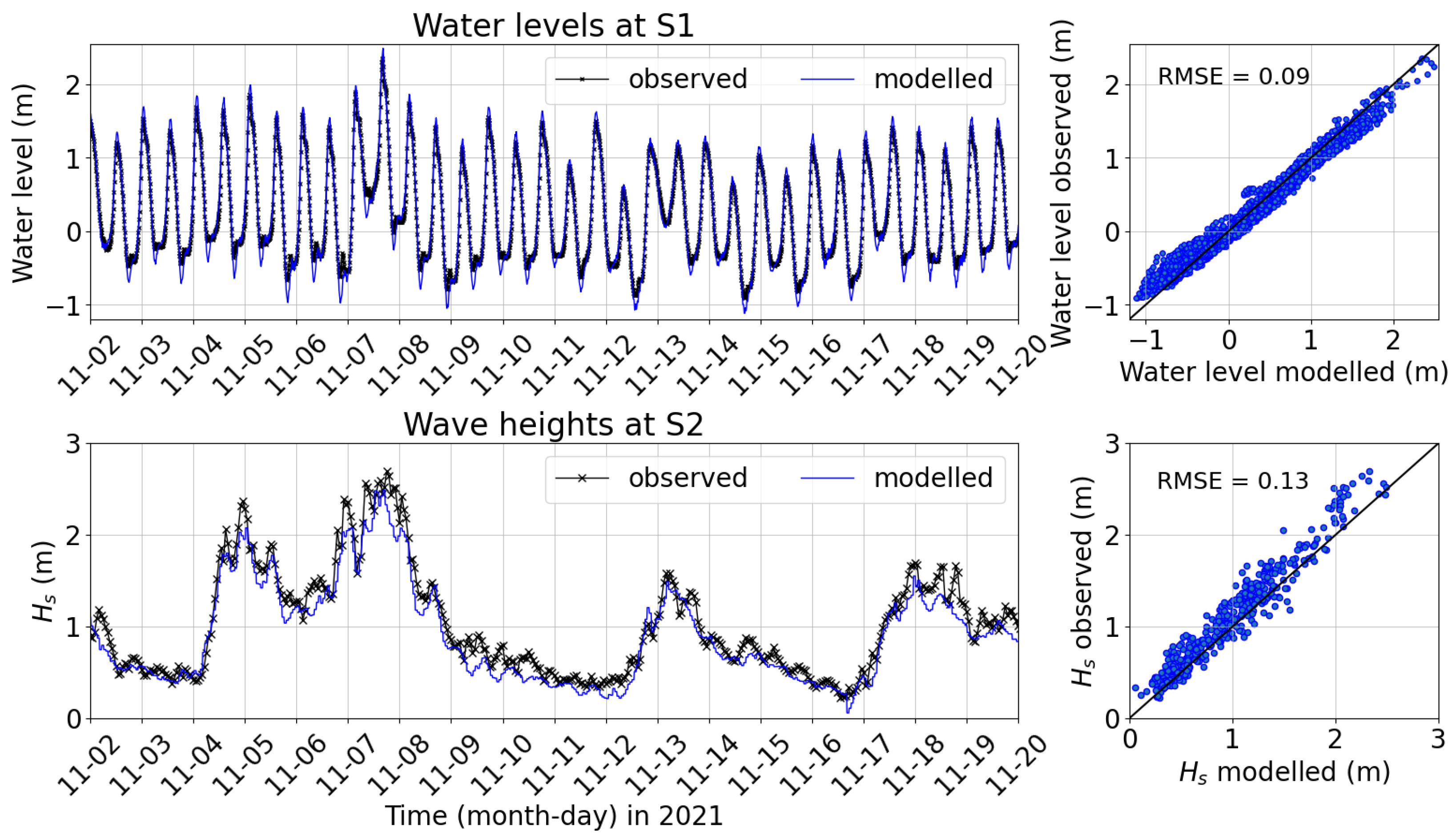
3.1.1. Hydrodynamics

First, a hydrodynamic hindcast was performed for the period from 1 November 2021 to 20 November 2021. The model was forced with observed water levels and wave heights obtained at measurement station 3 (Lichteiland Goeree; Figure 3). Hourly wind data were included, obtained at station 1. Discharge at the river discharge was derived using observed discharges into the RMD, at Lobith and Borgharen, and of the distributaries throughout the RMD.
Modeled water levels at station 1 were compared to observed water levels at roughly the same location. Similarly, wave propagation from the offshore boundary to the nearshore was hindcasted by comparing nearshore wave heights at station 2 (Figure 3). Predicted water levels and wave heights were line with expectations, both RMSE values lay within the statistical guidelines for estuarine model performance [59]. Over the hindcast at station 1, modeled depth-averaged peak flow velocities were 0.86 m/s during ebb and 0.48 m/s during flood. Data from the local port reports typical depth-averaged peak flow velocities at the same to vary between 0.5 and 1.0 m/s during ebb, and 0.55 and 1.35 m/s during flood, under varying offshore water levels and upstream discharges [60].

3.1.2. Morphological Patterns

Next, 1-year of morphological development is simulated with the reference simulation (Figure 4). Sedimentation is seen throughout the channel, with the exception of the estuarine mouth and the banks around the inlet. This resulted in an annual average accretion of 13.2 cm. This is in line with expectations: Literature reports the ‘natural’ annual accretion averaged over the Rotterdam Waterway to be 12.5 ± 2.5 cm over the period 2000–2019 [61]. Offshore sediment deposition can be seen in the extension of the channel, and the coastline experiences both erosion and accretion.

3.2. Changing Channel Depth

First, the impact of changing channel depth is assessed. The impact of channel deepening on channel morphology is displayed in Figure 5. Also, the sediment budget for the basin is given (Figure 5d), which indicates how much sediment has entered (positive sediment budget) or left (negative sediment budget) the estuarine basin in one year. As a consequence of increasing channel depth, retention of sediment in the estuarine channel increased in general. Erosion at the estuarine mouth decreased, and the area which experienced erosion moved offshore. In addition, deposition of sediment reduced offshore (Figure 5a). Channel average accretion increased from 10.8 cm to 14.2 cm for a channel depth of 13 m to 17 m, respectively, while sediment budget varied from 0.16 Mton ( 10 9 kg) to 0.50 Mton for the same scenarios (Figure 5c,d). The sediment budget approaches 0 Mton while accretion is still at 10.8 cm. This is because the system accumulates mud, which has a low density, while sand, which has a higher density, erodes and leaves the estuarine system.

3.3. Changing Wetland Width and Location

The plain view bed-level change after 1 year after implementation of wetlands with varying widths is displayed in Figure 6; channel depth is kept constant at 15 m. With an expanding wetland, erosion rates in the channel near the mouth and further inland increased, the sediment being transported offshore, where accretion increases. The channel banks start eroding resulting in a steeper profile between the channel and wetland. This is more visible in Figure 7, which shows the bed-level changes at the end of the year, averaged over the cross-sections, cross-channel, or the entire channel. Channel averaged bed-level change decreased from 13.2 to 3.6 cm, and the annual sediment budget for the entire basin decreased and even reversed, from 0.4 Mton to 0.42 Mton (Figure 6c,d).
Within the wetland, most bed-level changes were observed near the coastal boundary (Figure 6). Here, accretion was seen near the channel banks and higher up, while erosion was observed in between, which is most clearly visible in the wetland between 0–5 km in the lowest panel of Figure 6. This caused the initial, linear profile of the wetland to develop into a concave-up profile, typical for wave-dominant foreshores. Further upstream, slight accretion was observed throughout, which was most prominent near the channel. Here, cross-section average accretion rates were up to an order of magnitude smaller compared to those near the coast. When increasing the wetland width from 0.25 km to 1.0 km, average bed-level change in the wetland reduced from 5.2 cm to 2.6 cm (Figure 8). When deepening the channel from 13 to 17 m and keeping a constant 1 km wide wetland, average bed-level change over the entire wetland remained mostly constant at 2.5–2.8 cm, without any clear trend.
Next, the location of the wetland area was varied. Figure 9 shows how wetland restoration of 3 different segments of 5 km along the estuarine channel affects morphological trends, compared to no wetland area or a wetland along the entire 15 km segment. Following bed-level changes from the river boundary towards the offshore boundary (Figure 9b); upstream of the intervention, no change in morphological development was identified. Along the transect where wetland area was implemented, its presence caused net erosion which gradually increased downstream. Downstream from the intervention, the impact was still noticeable but less severe. In the coastal zone, the sedimentation increased. Wetlands along a 5 km segment decreased average channel accretion by 1.1–4.7 cm, while the same wetland area along the entire 15 km transect reduced average accretion by 9.5 cm. Comparably, adding wetlands along 5 km of the channel reduced annual sediment budget by 0.13–0.30 Mton, a wetland along the entire 15 km reduced the annual sediment budget by 0.81 Mton, which resulted in a negative sediment budget (Figure 9c,d). Notably, the wetlands implemented in the middle (5–10 km) resulted in most sediment retention, closest to the coast (0–5 km) resulted in the least amount of sediment being retained.

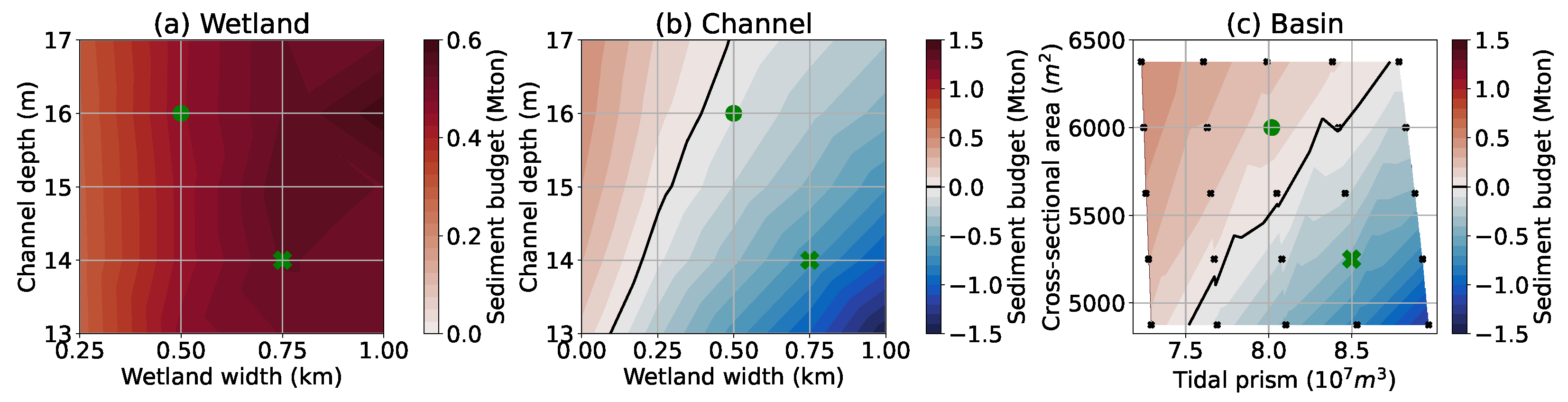
3.4. Channel Depth versus Wetland Width

Lastly, the combined impact of channel depth and wetland width were assessed (Figure 10). Results show how both interventions affect annual sediment budget in the wetland at the end of the year (Figure 10a). Sediment deposition in the wetland increased with wetland width and stayed mostly constant when varying the channel depth. However, under all simulated scenarios, net annual sediment budget within the wetland remained positive.
Moreover, for the 25 combined scenarios with varying channel depth and wetland area, the estuary’s spring ebb tidal prism (P) and the cross-sectional area below MSL (A) are evaluated in the inlet and compared to the annual sediment budget in the basin (Figure 10c). The inlet area A increases with channel depth, which results in lower flow velocities and more sediment retention in the basin. With a larger wetland area, the tidal prism increases, increasing tidal flow. Subsequently, due to wetland restoration, annual sediment budget lowers and the system gradually shifts from net importing sediment to net exporting sediment. A zero-contour line was identified where the system switched from a positive sediment budget to a negative sediment budget. Similar to P/A equilibrium relationships for inlet size, a value of P/A can be found where the annual sediment budget is close to zero. Here, this is with a P/A of ∼ 1.45 × 10 4 m/tide.

4. Discussion

Estuarine channels worldwide experience enhanced sedimentation rates because of traditional engineering solutions. For efficient port operations channels are deepened, and wetlands are embanked and claimed for human use. This paper reports on how changing channel depth and restoring wetlands affect sedimentation within the estuarine channel and how they affect morphological patterns in the wetland and in the entire estuarine basin.

4.1. Model Input Conditions

The model applies a cohesive (mud) and a non-cohesive (sand) sediment fraction. As a consequence of density differences in these sediment fractions, the estuarine channel can have a negative sediment budget while still experiencing accretion (Figure 7). Specifically, the system experiences a net export of sand but a net import of mud, which has a lower density. Mud is supplied by the river and is deposited throughout the estuarine basin. Exported sand mostly originates from the estuarine channel close to the sea, which is transported to the nearby wetland (if present) or the coastal zone. This is similar to findings on sand-mud behavior in a tide-dominant estuary, the Western Scheldt [62].
Although the model is applied in depth-averaged (2DH), in reality, density differences between fresh- and saltwater drive a residual current which influences the flow pattern over the depth, which promotes a tide-averaged landward flow near the bed. In 3D morphological models, this residual current is shown to promote sediment transport into the estuary from the coast [63], where 2DH models are not capable of capturing this residual current. A 3D adaptation of the presented model might result in the system being more prone to importing coastal sediments. Moreover, flocculation of mud particles in salt water may then also be accounted for (e.g., see [64]) since 3D modeling allows for accurate representation of the processes and interactions between fresh and saltwater necessary for the inclusion of flocculation processes.
Efforts were made to incorporate spatial and temporal varying vegetation cover to also represent vegetation establishment in the newly created wetland. Two approaches were tested. (1) A dynamic vegetation model, presented in [65], which includes processes to account for formation and decay of salt marsh vegetation over space and time; and (2) an approach using the empirical equation for the seaward extent of salt marsh vegetation cover based on mean tidal range identified by [53]. The latter does not account for vegetation establishment, and the vegetation cover in this approach is static over the 1-year simulation, as presented in Section 2.2.5 (this approach was used throughout the paper). Both approaches were tested in two morphodynamic models that mimic stretches of salt marshes in the Western Scheldt Estuary (a similar setup to the models presented in [54]). The vegetation module based on the empirical equation of [53] was able to predict seaward wetland extent well. However, the dynamic vegetation model is shown to be prone to overestimating seaward vegetation extent. In addition, the dynamic vegetation model relies on small grid cells to mimic the natural process of patch formation and vegetation establishment (∼10 m 2 ). With the larger cell sizes applied here (∼5000 m 2 ), the dynamic approach did not give desirable results for vegetation establishment. So also based on the larger cell sizes required to model an entire estuary as used here, the dynamic vegetation module did not contribute to a better approximation of the seaward salt marsh extent.

4.2. Model Timescale

Throughout the manuscript, 1-year morphological simulations were used to assess the initial response of the estuary’s morphology to human interventions. To gain insights into how this timescale affects model results, two scenarios were simulated for 5 consecutive years (channel depth = 15 m, intertidal wetland width = 1 km; Figure 11). Scenario (1) Without dredging: In this scenario, we simulate five years of morphological development without artificial interference. Scenario (2) With dredging: In this scenario, after each year of morphological development, the channel is dredged to restore the shape of the channel at the start of the year. The dredged sediments are removed from the model domain.
The intertidal wetland experiences the highest sedimentation rates in the first year. Subsequently, annual sedimentation rates reduce gradually while remaining positive. Notably, sedimentation is higher in the scenario with annual dredging (orange line; Figure 11a), indicating that dredging might promote accretion. Channel sedimentation rates remained constant in the dredged scenario but steadily increased in the scenario without dredging (Figure 11b). The scenario with annual dredging (orange and purple lines) experiences lower annual sedimentation rates in the channel compared to the scenario without dredging (green line). Over the long term, one would expect the opposite: When no dredging is performed and the channel depth decreases over time, annual sedimentation rates will reduce and converge to zero when channel depth reaches equilibrium. However, analysis of the model output shows that channel dredging, which is also applied upstream such that the channel depth is maintained throughout the domain, reduced the sediment flux into the estuary from upstream. Additionally, the sediment flux through the inlet towards the coast was higher in the scenario with dredging. This led to less total sedimentation in the channel but also in the basin (Figure 11b,c) in the scenario with dredging (orange + purple lines) versus the scenario without dredging (green line).

4.3. Steering Estuarine Morphology Using Large-Scale Interventions

Due to deepening of the estuarine channel, the channel experienced increased sedimentation (Figure 5), a trend that is observed in estuaries worldwide. Channels which are deepened below their equilibrium depth for navigational purposes can experience increased SSCs and require larger amounts of dredging is required to maintain the desired channel depth (examples hereof: [61,66,67,68]). When channel depth was varied, accretion of the wetland area remained mostly similar (Figure 8a). However, when 5 consecutive years were simulated (Figure 11), maintaining channel depth through dredging did increase sedimentation in the wetland, indicating that dredging to maintain channel depth can promote sedimentation rates in intertidal areas. In literature, dredging operations have been related to a retreat of salt marshes [69], but also to sedimentation of tidal flats and their creeks [6].
Within the results obtained here, the wetland always experienced a positive sediment budget (Figure 10a). This may be due to the choices made in the model setup, e.g., the initial linear intertidal cross-section and the 1-year simulation, as well as model assumptions reflecting a system with sufficient sediment supply. In other estuaries or under more extreme scenarios, deepening of the channel may reduce sediment supply to the wetland area to such an extent that it results in a negative sediment budget for the wetland area.
Addition of wetland area reduced sedimentation rates in the channel and in the estuarine basin (Figure 7c,d). The wetland area serves as sediment sink, retaining sediment which could otherwise accumulate in the channel. This is also visible in the results, where the wetland retained sediment in all scenarios (Figure 8). However, due to wetland restoration, the channel’s sediment budget was reduced by ∼0.6–1.3 Mton/year (highest values with lower channel depth; Figure 7), the sediment sink in the wetland accounts for only 0.2–0.4 Mton/year (Figure 10a), indicating that other processes play a substantial role in reducing channel sedimentation rates, which is discussed below.

4.4. Tidal Prism Cross-Sectional Area Relationship

The P/A relationship helps explain the impact of channel depth and wetland width on the annual sediment budget. Specifically, channel deepening increased the cross-sectional area (A), reducing all flow velocities in the estuary and enhancing sediment retention. Wetland restoration enlarged the tidal prism (P), which increased tidal flow velocities in the estuary. Consequently, due to wetland restoration the tendency of sediment to accumulate decreased which made the system more prone to erosion. In the performed simulations, the impact of wetland restoration on the tidal prism—and thus reducing the annual sediment budget—was more potent than the sediment accumulating on the wetland itself (and lowering channel sedimentation that way).
The changes in tidal prism (P) and cross-section area (A) due to large-scale interventions were also compared to see if the relationship between P and A can be used to predict sedimentation rates (Figure 10c). A clear relationship can be identified between P, A and the annual sediment budget: the annual sediment budget increases towards the top left (low P/A) and reduces towards the lower right (high P/A). Based on modeled results, the value for P/A at which the basin had a neutral sediment budget was ∼1.45× 10 4 m/tide. Literature indicates that P/A relationships for inlets are generally linear [58], which seems to be the case also when considering P and A compared to the annual sediment budget of the basin (Figure 10). Following the theory for equilibrium relationships in inlets, your inlet will remain in equilibrium if, e.g., a 10 % increase in cross-sectional area is compensated for by a 10 % increase in tidal prism. Similarly, the estuary’s annual sediment budget remains similar if channel deepening is compensated for with a proportional increase in the tidal prism, e.g., by increasing intertidal wetland area. However, more research is required to generalize these findings to other types of estuaries and a wider range of interventions.

4.5. Implications for Estuarine Management

Traditional engineering solutions, such as deepening of navigational channels and embanking and reclamation of wetland area, shift the estuarine channel towards a state more prone to sedimentation. As a consequence, the channels need constant dredging to maintain depths desired for port operations. Contrarily, wetland restoration—a nature-based solution—can reduce sedimentation rates, reducing the amount of dredging required. Specifically, wetlands serve as sediment sinks but, more substantially, increase the tidal prism which results in less sediment retention in the estuarine channel.
Moreover, our results indicate that wetland restoration mostly affected channel morphology locally (i.e., along the segment where the wetland is restored; Figure 9). The impact on channel accretion rates gradually decreased downstream of the restored wetland and upstream no significant impact was observed. As such, wetlands may be placed strategically at locations particularly prone to high sedimentation rates.
Additionally, Ref. [4] shows how restored wetlands may also serve as sediment sources available for erosion and thus can counter sediment starvation in estuaries under rising sea levels. However, as identified by [70], a fundamental knowledge gap exists still towards the morphological responses of estuaries under climate change impacts such as sea-level rise, let alone in combination with human interventions.
Although wetland restoration can reduce dredging maintenance within the navigational channel, results indicate that the channel banks and wave dominated wetlands can become prone to erosion (Figure 6 and Figure 7). The RMD system is already prone to bank erosion [61], similar to many other estuarine regions [11]. Hence, measures for bank protections or to steer wetland development might be required (e.g., see [11,19,71]).

5. Conclusions

In this paper, the short-term morphological response after two large-scale interventions in a highly engineered estuary is explored. We focused on (1) How channel deepening affects morphology in the coupled channel-wetland estuary system and (2) To what extent wetland restoration can steer channel morphology. An idealized 2D-morphological model was developed, reflecting a micro-tidal and wave-dominant estuary. Using 1-year morphological simulations, the system’s initial response to two large-scale interventions is assessed, altering channel depth and changing wetland area (i.e., reclaiming, restoring or creating wetlands).
(1) Results showed that after deepening of the channel from 13 m to 17 m (without wetland), sediment accretion rates increased by 31% within the channel, and the sediment budget of the wetland was mostly unaffected by channel depth. (2) The restored wetlands served as sediment sink, retaining sediment that could have accumulated in the channel otherwise. Furthermore, wetland restoration increased the tidal prism, which consequently impeded sedimentation in the estuarine channel. In this way, wetland restoration reduced sedimentation in the channel by 72 % (with a channel depth of 15 m and restored wetland width = 1 km). Further analysis was performed on the location of the wetland along the channel. This showed that wetland restoration mostly affects sedimentation of the channel locally (i.e., along the segment where the wetland is restored). As such, wetlands could be placed along channel segments particularly prone to sedimentation.
In conclusion, findings suggest that increased sedimentation rates in engineered estuaries worldwide, caused by channelization and channel deepening, could be compensated for by intertidal wetland restoration along the estuarine channel. As such, restoring wetland area could be considered to alleviate dredging operations at critical locations.

Author Contributions

Conceptualization, R.W.A.S.; methodology, R.W.A.S., T.M.D. and P.W.J.M.W.; software, R.W.A.S.; validation, R.W.A.S.; formal analysis, R.W.A.S.; investigation, R.W.A.S.; resources, R.W.A.S.; data curation, R.W.A.S.; writing—original draft preparation, R.W.A.S.; writing—review and editing, T.M.D., P.W.J.M.W., B.W.B. and S.J.M.H.H.; visualization, R.W.A.S.; supervision, T.M.D., B.W.B. and S.J.M.H.H.; project administration, R.W.A.S.; funding acquisition, B.W.B. and S.J.M.H.H. All authors have read and agreed to the published version of the manuscript.

Funding

This work is part of the Perspectief Program Saltisolutions, which is funded by NWO Domain Applied and Engineering Sciences in collaboration with private and public partners. Moreover, this work is a part of the Simon Stevin Master Grant of S.J.M.H. Hulscher. Part of publication is funded via the ‘LIVING DIKES—Realising Resilient and Climate-Proof Coastal Protection’ project (with project number NWA.1292.19.257) of the NWA research program ‘Research on Routes by Consortia (ORC)’, which is funded by the Netherlands Organization for Scientific Research (NWO).

Data Availability Statement

No new data were created or analyzed in this study. Data sharing is not applicable to this article.

Acknowledgments

This work used the Dutch national e-infrastructure with the support of the SURF Cooperative.

Conflicts of Interest

The authors declare no conflict of interest.

Appendix A

The Delft3D-FM modeling software is used to solve the hydrodynamic and morphodynamic processes in the model, as well as the impact of vegetation on these processes. Below, the governing equations are laid out. For more information, see the corresponding manuals [42,43,44].

Appendix A.1

In Delft3D-FM, the shallow water equations are solved under the assumption of incompressible fluid, hydrostatic pressure and the Boussinesq approximation (density differences are only included in the pressure term). In addition, this study applies the equation in 2DH (depth-averaged):
h t + h u x + h u y = 0
u t + u u x + v u y + g h y + 1 p 0 τ x x x + τ x y y + τ b x h = 0
v t + u v x + v v y + g h y + 1 p 0 τ y x x + τ y y y + τ b y h = 0
where u and v represent the velocity components in the x- and y-direction. p and p 0 the density and initial density, g the gravitational force, τ b the bed shear stress and h the water depth.
Vegetation impacts on the flow are included using the roughness predictor by [39], resulting in an increased roughness (C) and flow resistance of the vegetation ( λ ) in the vegetated areas based on vegetation height ( h v e g ) and vegetation density ( n b ), and is valid for emergent and submerged vegetation:
C = C b + g κ ln h h v e g 1 + C D n b h v e g C b 2 2 g
λ = C D n b h v e g h C b 2 C 2
where C b is the bed roughness, κ the von Kármán constant and C D the drag coefficient.

Appendix A.2

D-waves describes the evolution of the wave energy spectrum using the spectral action balance equation (using the third generation Simulating WAves Nearshore (SWAN) spectral wave model (based on [38]), following linear wave theory:
t N + x c x N + y c y N + σ c σ N + θ c θ N = S σ
where N is the action density, which changes over time and space in the x and y directions relative to the propagation velocity ( c x , c y ). The fourth term represents the frequency shifting due to depth and current variations and the fifth term represents refraction due to depth and currents. The source term (S) represents wave generation and dissipation and non-linear interactions between waves.
Vegetation induced wave dissipation ( S d i s , v e g ; [55]) is also included in this source term, predicted using:
S d i s , v e g = 2 π g 2 C D b v e g n b k σ s i n h 3 h v e g + 3 s i n h k h v e g 3 k c o s h 3 k h E t o t E ( σ , θ )
where C D is the drag coefficient, b v e g , n b and h v e g the diameter, density and height of the vegetation, k and σ the wave number and mean frequency, E t o t the total energy and E ( σ , θ ) the energy over the wave frequency and direction.

Appendix A.3

Appendix A.3.1. Cohesive Sediments

The D-Morphology module solves cohesive sediment transport by solving the advection-diffusion (mass-balance) equation in 2DH, assuming all cohesive transport is suspended:
c t + u c x + v c y x ϵ S , x c x y ϵ S , y c y = S
where c is the mass concentration of the cohesive fraction, u and v the flow velocity components in the x and y-direction, ϵ s is the respective eddy diffusivity, and S is the source and sink term related to the erosive and deposition fluxes at the bed.
The erosive and deposition fluxes are determined using the Partheniades–Krone formulations [40]:
E = M τ b , m a x τ c r , e 1 , for τ b , m a x > τ c r , e 0 , for τ b , m a x < τ c r , e
D = w s C 1 τ b , m a x τ c r , d , for τ b , m a x < τ c r , d 0 , for τ b , m a x > τ c r , d
where M is the erosion parameter, τ b , m a x is the maximum bed shear stress, τ c r , e and τ c r , d the critical bed shear stress for erosion and deposition w s the settling velocity, c the average sediment concentration.

Appendix A.3.2. Non-Cohesive Sediments

Non-cohesive sediment transport is based on the approach of [41], accounting for bed-load and suspended load, and both flow- and wave-processes on sediment transport. In 2D, the erosive and deposition fluxes are determined based on a relaxation towards an equilibrium concentration:
S = c e q c T
where c is the sediment concentration, c e q , the equilibrium concentration based on the sediment transport equations of [41], S the total net source and sink term and T the relaxation timescale based on the work of [72].
The approach from [41] differentiates sediment transport above and below a determined reference height, treated as suspended- and bed-load transport. Sediment concentrations in the water column are subsequently determined by the reference concentration at the reference height.

References

  1. Giosan, L.; Syvitski, J.; Constantinescu, S.; Day, J. Climate change: Protect the world’s deltas. Nature 2014, 516, 31–33. [Google Scholar] [CrossRef] [PubMed]
  2. Cox, J.; Lingbeek, J.; Weisscher, S.; Kleinhans, M. Effects of sea-level rise on dredging and dredged estuary morphology. J. Geophys. Res. Earth Surf. 2022, 127, 1–20. [Google Scholar] [CrossRef]
  3. Eslami, S.; Hoekstra, P.; Nguyen Trung, N.; Ahmed Kantoush, S.; Van Binh, D.; Duc Dung, D.; Tran Quang, T.; van der Vegt, M. Tidal amplification and salt intrusion in the Mekong Delta driven by anthropogenic sediment starvation. Sci. Rep. 2019, 9, 18746. [Google Scholar] [CrossRef] [PubMed]
  4. Leuven, J.R.F.W.; Pierik, H.J.; van der Vegt, M.; Bouma, T.J.; Kleinhans, M.G. Sea-level-rise-induced threats depend on the size of tide-influenced estuaries worldwide. Nat. Clim. Chang. 2019, 9, 986–992. [Google Scholar] [CrossRef]
  5. Costanza, R.; d’Arge, R.; de Groot, R.; Farber, S.; Grasso, M.; Hannon, B.; Limburg, K.; Naeem, S.; O’Neill, R.V.; Paruelo, J.; et al. The value of the world’s ecosystem services and natural capital. Nature 1997, 387, 253–260. [Google Scholar] [CrossRef]
  6. Du, J.L.; Yang, S.L.; Feng, H. Recent human impacts on the morphological evolution of the Yangtze River delta foreland: A review and new perspectives. Estuar. Coast. Shelf Sci. 2016, 181, 160–169. [Google Scholar] [CrossRef]
  7. Van Dijk, W.M.; Cox, J.R.; Leuven, J.R.; Cleveringa, J.; Taal, M.; Hiatt, M.R.; Sonke, W.; Verbeek, K.; Speckmann, B.; Kleinhans, M.G. The vulnerability of tidal flats and multi-channel estuaries to dredging and disposal. Anthr. Coasts 2021, 4, 36–60. [Google Scholar] [CrossRef]
  8. Syvitski, J.P.; Kettner, A.J.; Overeem, I.; Hutton, E.W.; Hannon, M.T.; Brakenridge, G.R.; Day, J.; Vörösmarty, C.; Saito, Y.; Giosan, L.; et al. Sinking deltas due to human activities. Nat. Geosci. 2009, 2, 681–686. [Google Scholar] [CrossRef]
  9. Schmitt, R.; Rubin, Z.; Kondolf, G. Losing ground-scenarios of land loss as consequence of shifting sediment budgets in the Mekong Delta. Geomorphology 2017, 294, 58–69. [Google Scholar] [CrossRef]
  10. de Jonge, V.N.; Schückel, U. Exploring effects of dredging and organic waste on the functioning and the quantitative biomass structure of the Ems estuary food web by applying Input Method balancing in Ecological Network Analysis. Ocean Coast. Manag. 2019, 174, 38–55. [Google Scholar] [CrossRef]
  11. Sanches Fernandes, L.F.; Sampaio Pinto, A.A.; Salgado Terencio, D.P.; Leal Pacheco, F.A.; Vitor Cortes, R.M. Combination of ecological engineering procedures applied to morphological stabilization of estuarine banks after dredging. Water 2020, 12, 391. [Google Scholar] [CrossRef]
  12. Cox, J.; Leuven, J.; Pierik, H.; van Egmond, M.; Kleinhans, M. Sediment deficit and morphological change of the Rhine–Meuse river mouth attributed to multi-millennial anthropogenic impacts. Cont. Shelf Res. 2022, 244, 104766. [Google Scholar] [CrossRef]
  13. Wang, Y.H.; Tang, L.Q.; Wang, C.H.; Liu, C.J.; Dong, Z.D. Combined effects of channel dredging, land reclamation and long-range jetties upon the long-term evolution of channel-shoal system in Qinzhou bay, SW China. Ocean Eng. 2014, 91, 340–349. [Google Scholar] [CrossRef]
  14. Pye, K.; Blott, S.J. The geomorphology of UK estuaries: The role of geological controls, antecedent conditions and human activities. Estuar. Coast. Shelf Sci. 2014, 150, 196–214. [Google Scholar] [CrossRef]
  15. Dunn, F.E.; Darby, S.E.; Nicholls, R.J.; Cohen, S.; Zarfl, C.; Fekete, B.M. Projections of declining fluvial sediment delivery to major deltas worldwide in response to climate change and anthropogenic stress. Environ. Res. Lett. 2019, 14, 084034. [Google Scholar] [CrossRef]
  16. Chen, Y.; Li, Y.; Thompson, C.; Wang, X.; Cai, T.; Chang, Y. Differential sediment trapping abilities of mangrove and saltmarsh vegetation in a subtropical estuary. Geomorphology 2018, 318, 270–282. [Google Scholar] [CrossRef]
  17. Kirwan, M.L.; Guntenspergen, G.R.; D’Alpaos, A.; Morris, J.T.; Mudd, S.M.; Temmerman, S. Limits on the adaptability of coastal marshes to rising sea level. Geophys. Res. Lett. 2010, 37. [Google Scholar] [CrossRef]
  18. Temmerman, S.; Meire, P.; Bouma, T.J.; Herman, P.M.; Ysebaert, T.; De Vriend, H.J. Ecosystem-based coastal defence in the face of global change. Nature 2013, 504, 79–83. [Google Scholar] [CrossRef]
  19. Hu, Z.; Borsje, B.W.; van Belzen, J.; Willemsen, P.W.; Wang, H.; Peng, Y.; Yuan, L.; De Dominicis, M.; Wolf, J.; Temmerman, S.; et al. Mechanistic modeling of marsh seedling establishment provides a positive outlook for coastal wetland restoration under global climate change. Geophys. Res. Lett. 2021, 48, e2021GL095596. [Google Scholar] [CrossRef]
  20. Nesshöver, C.; Assmuth, T.; Irvine, K.N.; Rusch, G.M.; Waylen, K.A.; Delbaere, B.; Haase, D.; Jones-Walters, L.; Keune, H.; Kovacs, E.; et al. The science, policy and practice of nature-based solutions: An interdisciplinary perspective. Sci. Total Environ. 2017, 579, 1215–1227. [Google Scholar] [CrossRef]
  21. Ganju, N.K. Marshes are the new beaches: Integrating sediment transport into restoration planning. Estuaries Coasts 2019, 42, 917–926. [Google Scholar] [CrossRef]
  22. Wiberg, P.L.; Fagherazzi, S.; Kirwan, M.L. Improving predictions of salt marsh evolution through better integration of data and models. Annu. Rev. Mar. Sci. 2020, 12, 389–413. [Google Scholar] [CrossRef] [PubMed]
  23. Dam, G.; van der Wegen, M.; Labeur, R.J.; Roelvink, D. Modeling centuries of estuarine morphodynamics in the Western Scheldt estuary. Geophys. Res. Lett. 2016, 43, 3839–3847. [Google Scholar] [CrossRef]
  24. Luan, H.L.; Ding, P.X.; Wang, Z.B.; Ge, J.Z. Process-based morphodynamic modeling of the Yangtze Estuary at a decadal timescale: Controls on estuarine evolution and future trends. Geomorphology 2017, 290, 347–364. [Google Scholar] [CrossRef]
  25. Elmilady, H.; Van der Wegen, M.; Roelvink, D.; Jaffe, B. Intertidal area disappears under sea level rise: 250 years of morphodynamic modeling in San Pablo Bay, California. J. Geophys. Res. Earth Surf. 2019, 124, 38–59. [Google Scholar] [CrossRef]
  26. Nahon, A.; Bertin, X.; Fortunato, A.B.; Oliveira, A. Process-based 2DH morphodynamic modeling of tidal inlets: A comparison with empirical classifications and theories. Mar. Geol. 2012, 291, 1–11. [Google Scholar] [CrossRef]
  27. Duong, T.M.; Ranasinghe, R.; Walstra, D.; Roelvink, D. Assessing climate change impacts on the stability of small tidal inlet systems: Why and how? Earth-Sci. Rev. 2016, 154, 369–380. [Google Scholar] [CrossRef]
  28. Duong, T.M.; Ranasinghe, R.; Luijendijk, A.; Walstra, D.; Roelvink, D. Assessing climate change impacts on the stability of small tidal inlets: Part 1-Data poor environments. Mar. Geol. 2017, 390, 331–346. [Google Scholar] [CrossRef]
  29. Duong, T.M.; Ranasinghe, R.; Thatcher, M.; Mahanama, S.; Wang, Z.B.; Dissanayake, P.K.; Hemer, M.; Luijendijk, A.; Bamunawala, J.; Roelvink, D.; et al. Assessing climate change impacts on the stability of small tidal inlets: Part 2-Data rich environments. Mar. Geol. 2018, 395, 65–81. [Google Scholar] [CrossRef]
  30. van der Wegen, M.; Dastgheib, A.; Roelvink, J. Morphodynamic modeling of tidal channel evolution in comparison to empirical PA relationship. Coast. Eng. 2010, 57, 827–837. [Google Scholar] [CrossRef]
  31. Rijkswaterstaat. Kenmerkende Waarden Getijgebied 2011.0; Report; RWS: Utrecht, The Netherlands, 2013.
  32. Grasmeijer, B.; Huisman, B.; Luijendijk, A.; Schrijvershof, R.; van der Werf, J.; Zijl, F.; de Looff, H.; de Vries, W. Modelling of annual sand transports at the Dutch lower shoreface. Ocean Coast. Manag. 2022, 217, 105984. [Google Scholar] [CrossRef]
  33. Reinson, G.E. Transgressive barrier island and estuarine systems. In Facies Models Response to Sea Level Change; Geological Association of Canada: St. John’s, NL, Canada, 1992; pp. 179–194. [Google Scholar]
  34. Hijma, M.P.; Cohen, K.M.; Hoffmann, G.; Van der Spek, A.J.; Stouthamer, E. From river valley to estuary: The evolution of the Rhine mouth in the early to middle Holocene (western Netherlands, Rhine-Meuse delta). Neth. J. Geosci. 2009, 88, 13–53. [Google Scholar] [CrossRef]
  35. Paalvast, P.; van der Velde, G. Long term anthropogenic changes and ecosystem service consequences in the northern part of the complex Rhine-Meuse estuarine system. Ocean Coast. Manag. 2014, 92, 50–64. [Google Scholar] [CrossRef]
  36. Pierik, H.J.; Stouthamer, E.; Schuring, T.; Cohen, K.M. Human-caused avulsion in the Rhine-Meuse delta before historic embankment (The Netherlands). Geology 2018, 46, 935–938. [Google Scholar] [CrossRef]
  37. Gouw, M.J.; Hijma, M.P. From apex to shoreline: Fluvio-deltaic architecture for the Holocene Rhine–Meuse delta, the Netherlands. Earth Surf. Dyn. 2022, 10, 43–64. [Google Scholar] [CrossRef]
  38. Booij, N.; Ris, R.C.; Holthuijsen, L.H. A third-generation wave model for coastal regions: 1. Model description and validation. J. Geophys. Res. Ocean. 1999, 104, 7649–7666. [Google Scholar] [CrossRef]
  39. Baptist, M.; Babovic, V.; Rodríguez Uthurburu, J.; Keijzer, M.; Uittenbogaard, R.; Mynett, A.; Verwey, A. On inducing equations for vegetation resistance. J. Hydraul. Res. 2007, 45, 435–450. [Google Scholar] [CrossRef]
  40. Partheniades, E.J. Erosion and deposition of cohesive soils. J. Hydraul. Div. 1965, 91, 105–139. [Google Scholar] [CrossRef]
  41. Van Rijn, L. Principles of Sediment Transport in Rivers, Estuaries and Coastal Seas; Aqua Publications: Blokzijl, The Netherlands, 1993; Volume 1006. [Google Scholar]
  42. Deltares. D-Flow user manual. In Delft3D FM Suite; Deltares: Delft, The Netherlands, 2021. [Google Scholar]
  43. Deltares. D-WAVE user manual. In Delft3D FM Suite; Deltares: Delft, The Netherlands, 2021. [Google Scholar]
  44. Deltares. D-Morphology user manual. In Delft3D FM Suite; Deltares: Delft, The Netherlands, 2021. [Google Scholar]
  45. Dean, R.G. Equilibrium beach profiles: Characteristics and applications. J. Coast. Res. 1991, 7, 53–84. [Google Scholar]
  46. Van der Spek, A.; Van der Werf, J.; Grasmeijer, B.; Schrijvershof, R.; Vermaas, T. The lower shoreface of the Dutch coast—An overview. Ocean Coast. Manag. 2022, 230, 106367. [Google Scholar] [CrossRef]
  47. Kreischer. EN: Deepening Nieuwe Waterweg, Report on Fieldwork and Labresearch; Report (dutch); Gemeentewerken Rotterdam: Rotterdam, The Netherlands, 2014. [Google Scholar]
  48. Temmerman, S.; Bouma, T.J.; Govers, G.; Wang, Z.B.; De Vries, M.B.; Herman, P.M.J. Impact of vegetation on flow routing and sedimentation patterns: Three-dimensional modeling for a tidal marsh. J. Geophys. Res. Earth Surf. 2005, 110. [Google Scholar] [CrossRef]
  49. Sloff, K.; van der, R.S.; Huismans, Y.; Fuhrhop, H. Morphological Model of the RhineMeuse Delta; Report; Deltares: Delft, The Netherlands, 2012. [Google Scholar]
  50. RWS. National Water Authority; Live Database; RWS: Utrecht, The Netherlands, 2022.
  51. Klijn, F.; Hegnauer, M.; Beersma, J.; Sperna Weiland, F. Wat Betekenen de Nieuwe Klimaatscenario’s Voor de Rivierafvoeren van Rijn en Maas? Samenvatting van Onderzoek Met GRADE Naar Implicaties van Nieuwe klimaatprojecties voor Rivierafvoeren; Deltares & KNMI: Delft, The Netherlands, 2015. [Google Scholar]
  52. Snippen, E.; Fioole, A.; Geelen, H.; Kamsteeg, A.; Spijk, A.; Visser, T. Sediment in (be)weging. In Sedimentbalans Rijn-Maasmonding Periode 1990–2000; Report, RWS-RIZA, Afdeling WRE; RWS: Utrecht, The Netherlands, 2005. [Google Scholar]
  53. Balke, T.; Stock, M.; Jensen, K.; Bouma, T.J.; Kleyer, M. A global analysis of the seaward salt marsh extent: The importance of tidal range. Water Resour. Res. 2016, 52, 3775–3786. [Google Scholar] [CrossRef]
  54. Willemsen, P.; Smits, B.; Borsje, B.; Herman, P.; Dijkstra, J.; Bouma, T.; Hulscher, S. Modelling decadal salt marsh development: Variability of the salt marsh edge under influence of waves and sediment availability. Water Resour. Res. 2022, 58, e2020WR028962. [Google Scholar] [CrossRef]
  55. Suzuki, T.; Arikawa, T. Numerical analysis of bulk drag coefficient in dense vegetation by immersed boundary method. In Proceedings of the 32nd International Conference on Coastal Engineering, ICCE 2010, Shanghai, China, 30 June–5 July 2010. [Google Scholar]
  56. Vuik, V.; Jonkman, S.N.; Borsje, B.W.; Suzuki, T. Nature-based flood protection: The efficiency of vegetated foreshores for reducing wave loads on coastal dikes. Coast. Eng. 2016, 116, 42–56. [Google Scholar] [CrossRef]
  57. Jarrett, J.T. Tidal Prism-Inlet Area Relationships; US Department of Defense, Department of the Army, Corps of Engineers: Washington, DC, USA, 1976; Volume 3.
  58. Stive, M.J.; Rakhorst, R. Review of empirical relationships between inlet cross-section and tidal prism. J. Water Resour. Environ. Eng. 2008, 23, 89–95. [Google Scholar]
  59. Williams, J.J.; Esteves, L.S. Guidance on Setup, Calibration, and Validation of Hydrodynamic, Wave, and Sediment Models for Shelf Seas and Estuaries. Adv. Civ. Eng. 2017, 2017, 5251902. [Google Scholar] [CrossRef]
  60. Port of Rotterdam. HydroMeteoBundel nr. 4 1; report; Port of Rotterdam: Rotterdam, The Netherlands, 2012. [Google Scholar]
  61. Cox, J.R.; Huismans, Y.; Knaake, S.; Leuven, J.; Vellinga, N.; van der Vegt, M.; Hoitink, A.; Kleinhans, M. Anthropogenic Effects on the Contemporary Sediment Budget of the Lower Rhine-Meuse Delta Channel Network. Earth’s Future 2021, 9, e2020EF001869. [Google Scholar] [CrossRef]
  62. Dam, G.; Van der Wegen, M.; Taal, M.; Van der Spek, A. Contrasting behaviour of sand and mud in a long-term sediment budget of the Western Scheldt estuary. Sedimentology 2022, 69, 2267–2283. [Google Scholar] [CrossRef]
  63. Zhou, Z.; Chen, L.; Tao, J.; Gong, Z.; Guo, L.; van der Wegen, M.; Townend, I.; Zhang, C. The role of salinity in fluvio-deltaic morphodynamics: A long-term modelling study. Earth Surf. Process. Landforms 2020, 45, 590–604. [Google Scholar] [CrossRef]
  64. Tarpley, D.R.N.; Harris, C.K.; Friedrichs, C.T.; Sherwood, C.R. Tidal Variation in Cohesive Sediment Distribution and Sensitivity to Flocculation and Bed Consolidation in An Idealized, Partially Mixed Estuary. J. Mar. Sci. Eng. 2019, 7, 334. [Google Scholar] [CrossRef]
  65. Temmerman, S.; Bouma, T.J.; Van de Koppel, J.; Van der Wal, D.D.; De Vries, M.B.; Herman, P.M.J. Vegetation causes channel erosion in a tidal landscape. Geology 2007, 35, 631–634. [Google Scholar] [CrossRef]
  66. Van Maren, D.; van Kessel, T.; Cronin, K.; Sittoni, L. The impact of channel deepening and dredging on estuarine sediment concentration. Cont. Shelf Res. 2015, 95, 1–14. [Google Scholar] [CrossRef]
  67. Luan, H.L.; Ding, P.X.; Wang, Z.B.; Ge, J.Z.; Yang, S.L. Decadal morphological evolution of the Yangtze Estuary in response to river input changes and estuarine engineering projects. Geomorphology 2016, 265, 12–23. [Google Scholar] [CrossRef]
  68. Dijkstra, Y.M.; Schuttelaars, H.M.; Schramkowski, G.P.; Brouwer, R.L. Modeling the transition to high sediment concentrations as a response to channel deepening in the Ems River Estuary. J. Geophys. Res. Ocean. 2019, 124, 1578–1594. [Google Scholar] [CrossRef]
  69. Cox, R.; Wadsworth, R.; Thomson, A. Long-term changes in salt marsh extent affected by channel deepening in a modified estuary. Cont. Shelf Res. 2003, 23, 1833–1846. [Google Scholar] [CrossRef]
  70. Khojasteh, D.; Glamore, W.; Heimhuber, V.; Felder, S. Sea level rise impacts on estuarine dynamics: A review. Sci. Total Environ. 2021, 780, 146470. [Google Scholar] [CrossRef] [PubMed]
  71. Siemes, R.W.A.; Borsje, B.W.; Daggenvoorde, R.J.; Hulscher, S.J.M.H. Artificial Structures Steer Morphological Development of Salt Marshes: A Model Study. J. Mar. Sci. Eng. 2020, 8, 326. [Google Scholar] [CrossRef]
  72. Galappatti, R. A depth integrated model for suspended transport. In Communications on Hydraulics 1983-07; Delft University of Technology: Delft, The Netherlands, 1983. [Google Scholar]
Figure 1. The schematized model domain, and a visualization of the study area upon which model assumptions are based. (a) Top view of the Rotterdam Waterwaywithin the red box, and the locations of used measurement stations (S1–S3). Satellite image from Google Earth. (b) Top view of the schematized bathymetry, locations of the hydrodynamic forcings and locations used to compare with observations (S1 and S2). (c) Cross-section representation of the large-scale interventions implemented in the model domain (as explained in detail in Section 2.3).
Jmse 11 02150 g001
Figure 2. Forcing for river discharge regime (Left) and wave climate (Middle and Right) resembling a reference year in the Rotterdam Waterway. Wave directions are relative to North.
Jmse 11 02150 g002
Figure 3. Observed and modeled water levels (Top) and wave heights (Bottom) in the Rotterdam Waterway estuary, at measurement locations S1 and S2, respectively (locations shown in Figure 1). The right figures compare the time series, the left figures display scatter plots and the RMSE for both comparisons.
Jmse 11 02150 g003
Figure 4. Bed-level change after one year within the reference scenario.
Jmse 11 02150 g004
Figure 5. Effect of channel depth on annual morphological bed-level change. (a) Bed-level change averaged over the cross-sections, (b) cross-channel averaged bed-level change, (c) Average bed-level change over the entire channel and (d) Sediment budget for the entire estuarine basin. The solid black line in figure (a,b) show the zero-contour line. Note: No wetland is present in these scenarios. The grey box in figure (c,d) indicate the reference scenario.
Jmse 11 02150 g005
Figure 6. Plain view of bed-level change after one year with a wetland width of 0.25 km, 0.5 km, 0.75 km and 1 km (from top to bottom). The black dotted lines display mean low water (MLW) and mean high water (MHW), the boundaries of the initial intertidal wetland area. Channel depth is kept constant at 15 m.
Jmse 11 02150 g006
Figure 7. Effect of wetland width on annual morphological bed-level change. (a) Bed-level change averaged over the cross-sections, (b) cross-channel averaged bed-level change, (c) Average bed-level change over the entire channel and (d) Sediment budget for the entire estuarine basin. The solid black line in figure (a,b) show the zero-contour line. The grey box in figure (c,d) indicate the reference scenario. Channel depth is kept constant at 15 m.
Jmse 11 02150 g007
Figure 8. (a) Effect of channel depth on average bed-level change within the wetland area, with a constant wetland width of 1.0 km. (b) Effect of wetland width on average bed-level change within the wetland, whereby channel depth is constant at 15 m.
Jmse 11 02150 g008
Figure 9. The effect of variation in wetland location on estuarine morphology. (a) Cross-sectional average bed-level change without a wetland area present and (b) difference herein due to implementing wetlands along both banks. Green striped boxes indicate the along-shore location of the restored wetland. Impact of wetland location on (c) channel average bed-level change and (d) Basin total sediment budget. The grey box in figure (c,d) indicate the reference scenario.
Jmse 11 02150 g009
Figure 10. Combined impact of channel depth and wetland width on estuarine-wide morphology after one year. Annual sediment budget within (a) the wetland and (b) the channel. Hereby, each grid point represents a model simulation. (c) Annual sediment budget of the entire estuary as a function of the tidal prism (P) and cross-sectional area (A) within the inlet. The black dots/arrows represent model simulations. The ones in green visualize how scenarios in the different plots relate.
Jmse 11 02150 g010
Figure 11. Bed-level change in the intertidal wetland and channel (a,b), and change in sediment volume in the entire basin (c) at the end of each year over 5 years. For both scenarios, channel depth = 15 m and total wetland width = 1 km. Dredging is performed at the end of each year, restoring the channel to its initial shape. Dredged sediments are removed from the model domain, hence the orange line in Figure (b) is equal to zero.
Jmse 11 02150 g011
Table 1. Overview of key parameter values applied in the morphological model.
SymbolVariableUnitValueReference
Hydrodynamic parameters
n f l o w Manning friction coefficients m 1 / 3 0.023[42]
n w a v e JONSWAP friction coefficients m 1 / 3 0.038[42]
Morphological parameters
ρ s o i l Specific densitykg m 3 2650[42]
ρ s a n d Dry bed density sandkg m 3 1600[42]
ρ m u d Dry bed density mudkg m 3 500[42]
D 50 s a n d Median grain size sand μ m200[47]
w s Settling velocity mudmm s 1 0.25[42]
τ c r i t , m u d Critical stress for erosion of mudN/ m 2 0.5[42]
Vegetation parameters
C d v e g Vegetation drag coefficient 0.7[42]
d v e g Uniform vegetation stem diametermm4.3[48]
H v e g Uniform vegetation heightm0.5[48]
KMax. stem densityStems m 2 1200[48]
Table 2. Overview of scenarios within the idealized estuarine domain. Underlined is the reference scenario, most closely representing the study area in recent history. * Lateral location of the wetland indicates the range between which wetland area is implemented, whereby 0 km is directly landwards of the coast.
Scenarios
1. Channel depth ( C d ; m)1314151617
2. Total intertidal wetland width ( I w ; km)00.250.50.751.0
3. Lateral wetland location * (km–km)0–150–55–1010–15
Disclaimer/Publisher’s Note: The statements, opinions and data contained in all publications are solely those of the individual author(s) and contributor(s) and not of MDPI and/or the editor(s). MDPI and/or the editor(s) disclaim responsibility for any injury to people or property resulting from any ideas, methods, instructions or products referred to in the content.

