Impacts of Arctic Sea Fog on the Change of Route Planning and Navigational Efficiency in the Northeast Passage during the First Two Decades of the 21st Century

Abstract

Under the background of climate change, the Northeast Passage’s navigability is on the rise. Arctic sea fog significantly influences navigational efficiency in this region. Existing research primarily focuses on routes accumulating the lowest distance, neglecting routes with the lowest time and sea fog’s influence on route planning and navigational efficiency. This study compares the fastest and shortest routes and analyzes Arctic sea fog’s impact on the Northeast Passage from June to September (2001–2020). The results show that coastal areas are covered with less sea ice under notable monthly variations. Sea fog frequency is highest near coasts, declining with latitude. September offers optimal navigation conditions due to minimal ice and fog. When only sea ice is considered, the fastest route is approximately 4 days quicker than the shortest. The shortest route has migrated towards the higher latitude over two decades, while the fastest route remains closer to the Russian coast. Adding the impact of sea fog on the fastest route, the speed decreased by 30.2%, increasing sailing time to 45.1%. The new fastest route considering both sea ice and sea fog achieved a 13.9% increase in sailing speed and an 11.5% reduction in sailing time compared to the original fastest route.

1. Introduction

The Arctic’s rapid warming has enhanced the navigability of the Northeast Passage, underscoring the region’s growing significance in the maritime transportation industry. Satellite data from 1979 to 2017 indicates a decrease in sea ice extent in September by 13% per decade [1]. In certain Arctic regions, the average sea ice thickness has decreased by 2 m in 60 years (1958–2018) [2]. Predictive models suggest that the Arctic will experience ice-free months before 2050 [3]. This reduction in sea ice has extended the navigational season and enhanced the viability of the Northeast Passage [4,5,6,7,8,9].

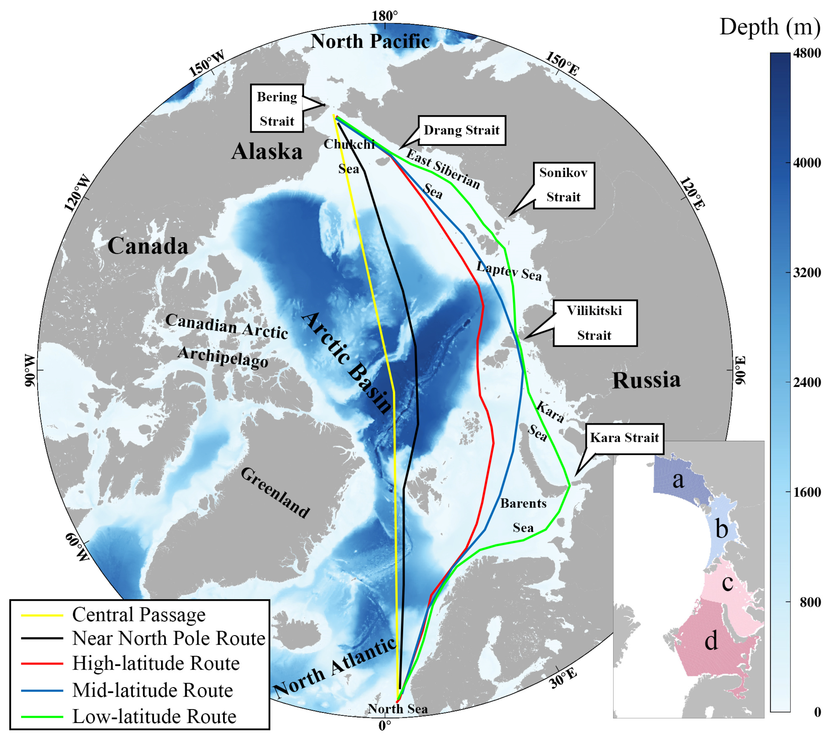
In 2020, the Protection of the Arctic Marine Environment Working Group (PAME) reported a 25% growth in Arctic shipping from 2013 to 2019 [10]. Trans-Arctic shipping routes that connect the northern Pacific and Atlantic Oceans are primarily divided into the Northeast Passage (NEP), the Northwest Passage (NWP), and the Central Passage [9]. Among them, the NEP stands out due to its minimal ice cover and optimal navigability. Compared to the conventionally used Suez Canal route, the NEP can reduce sailing distances by 15% to 50% [11,12,13]. Broadly speaking, the NEP encompasses four primary routes: the low-latitude route, the mid-latitude route, the high-latitude route, and the near North Pole route [14,15]. However, in a narrower sense, the NEP only includes the low-latitude and mid-latitude routes (Figure 1).

Recent years have seen a surge in research concerning the NEP. Nevertheless, most of these studies primarily rely on sea ice data to evaluate navigational feasibility in various Arctic regions, or to plan the least-cost route accumulating the lowest total distance (the shortest route) or time (the fastest route). Some of these studies have investigated alterations in sea ice and the navigational probability in the future NEP [16,17,18,19], yet lack comprehensive route planning. Li et al. assessed navigational risks for the future NEP, but their focus was limited to a scenario with extremely high radiative forcing (SSP5-8.5) [20]. Using the Arctic Transport Accessibility Model (ATAM), Wei et al. determined the steadily increasing probability of successful navigation in the NEP for the 21st century. However, despite September was considered the optimal month for navigation, the maximum navigational likelihood for a Polar Class 6 icebreaker (PC6) under the SSP5-8.5 scenario was only 67.5% [21]. In contrast, Min et al. analyzed variations in navigable windows and sailing time in the NEP spanning 2015 to 2100. They predicted that by the 2070s, the PC6 should be capable of navigating through the NEP all year round [4]. Melia et al. utilized CMIP5 sea ice data to plan the fastest route for the NEP from 2015 to 2100. Their findings suggest a consistent reduction in sailing time over 85 years, with the PC6 likely to enjoy a minimum 10-month shipping season in the NEP by the end of this century [22].

Arctic sea fog substantially influences the navigational efficiency of the NEP, especially in the planning of the fastest route. The appearance of sea fog in the Arctic significantly limits the visibility within affected regions, making it more challenging to determine the presence of ice conditions and endangering navigation. Consequently, vessels traversing sea ice areas are compelled to reduce their speed when encountering sea fog, to ensure the safety of navigation, resulting in increased time and economic costs of sailing. The absence of continuous and comprehensive observational data on Arctic sea fog has constrained research regarding its impact on Arctic navigability. Nam et al. attempted to quantify the deceleration effects of different Arctic weather conditions and apply them in NEP route simulation, but failed to adequately address the influence of sea fog on route selection and navigational efficiency [23]. Song et al. explored how sea fog frequency (SFF) affects the sailing time of a predetermined shortest route based on Coupled Model Inter-comparison Project Phase 5 (CMIP5) sea ice data, but their analysis lacked further analysis of specific routes [24].

Given that existing studies do not adequately elucidate the influence of Arctic sea fog on route planning and navigational efficiency, our study utilizes the Polar Operational Limit Assessment Risk Indexing System (POLARIS) and focuses on the PC6 as an example. We quantify the navigational risk of a PC6 in the NEP and plan the fastest route based on observational sea ice data and simulated sea fog data, then assess the further impact of Arctic sea fog on route planning and navigational efficiency in the NEP.

2. Data and Methods

2.1. Arctic Sea Ice and Sea Fog Data

In this study, both sea ice concentration (SIC) and sea ice thickness (SIT) data are necessary for the analysis of route planning and navigational efficiency. For SIC, we utilized Bootstrap sea ice concentration data Version 3, derived from the Scanning Multichannel Microwave Radiometer (SMMR), the Special Sensor Microwave/Imager (SSM/I) sensors, and the Special Sensor Microwave Imager/Sounder (SSMIS) on multiple satellites [25]. For SIT, the PIOMAS sea ice thickness reanalysis data were used [26,27]. Both the monthly SIC and SIT data have a resolution of 25 km.

SFF is defined as the percentage of foggy days in each month, where we classify foggy days as those with visibility of less than 1 km, ensuring that sea fog has a sufficient effect on the deceleration of the vessels [24]. The SFF data are derived from Arctic sea fog data based on the Polar-optimized version of the Weather Research and Forecasting Model (PWRF) with 6 hourly atmospheric fields from ERA-Interim reanalysis data sets (PWRF-ERA) provided by the Ocean University of China, with a spatial resolution of 50 km.

SFF data suggest a higher frequency of occurrence for Arctic sea fog from June through September. Concurrently, climate models show that the navigational probability of the NEP begins to appear from June every year [4,21,22]. Given these findings, we focus on the period spanning June to September over the initial two decades of the 21st century. Furthermore, we refer to the Arctic sea division by the National Snow and Ice Data Center (NSIDC) and choose the East Siberian Sea, Laptev Sea, Kara Sea, and Barents Sea (Figure 1) to further analyze variations in SFF in each region of the NEP [28].

2.2. Arctic Shipping Route Calculation

2.2.1. The Shortest Route

In our research, the POLARIS is used to quantify navigational risk in the NEP. The POLARIS, released by the International Maritime Organization in 2016, is currently the latest mechanism for evaluating navigational risks in ice-covered waters. This system integrates the advantages of the Canadian Arctic Ice Navigation System, the Russian Ice Navigation Permit, and other coastal traffic management agencies to include a more comprehensive vessel type and more detailed sea ice classification in the calculations, so it has a more refined level of risk quantification.

The risk value (RV) of a PC6 is obtained based on the SIT and the vessel’s icebreaking capability. Subsequently, the risk index outcome (RIO) is ascertained based on both RV and SIC. Regions with RIOs greater than or equal to 0 were considered navigable, higher RIO values indicate safer navigational conditions in a given region, whereas values less than 0 indicate the regions’ impassability. The RIO is used to plan the least-cost path accumulating the lowest total distance [29], which is also referred to as the shortest route (Route S). The starting and ending points of the route in this study are the Bering Strait and the Rotterdam, respectively. The formula for determining RIO is delineated below:

$$\mathrm{RIO}{\mathrm{s}}_{\mathrm{v}}={\displaystyle \sum {\mathrm{C}}_{\mathrm{T}}\times \mathrm{R}{\mathrm{V}}_{\mathrm{V},\mathrm{T}}},$$

(1)

The subscript T represents SIT, V represents vessel type, ${\mathrm{C}}_{\mathrm{T}}$ refers to the ice concentration corresponding to T-thickness sea ice in a certain region, and ${\mathrm{RV}}_{\mathrm{V},\mathrm{T}}$ refers to the RV of V-type vessels navigating in the area covered by T-thickness sea ice. It is worth noting that in the POLARIS, there are two types of sea ice with different RVs in the 120–200 cm thickness range, and there is a lack of RV for the 200–250 cm thickness range. Therefore, this study used the RV of thick first-year ice as the RV for the 120–200 cm and the RV of second-year ice for the 200–250 cm. The relationship between SIT and RV is:

$$\mathrm{R}{\mathrm{V}}_{\mathrm{P}\mathrm{C}6}=\{\begin{array}{l}3,\mathrm{SIT}=0\mathrm{cm}\\ 2,0\mathrm{cm}<\mathrm{SIT}\le 50\mathrm{cm}\\ 1,50\mathrm{cm}\le \mathrm{SIT}\le 95\mathrm{cm}\\ 0,95\mathrm{cm}\le \mathrm{SIT}\le 120\mathrm{cm}\\ -1,120\mathrm{cm}\le \mathrm{SIT}\le 200\mathrm{cm}\\ \begin{array}{l}-2,200\mathrm{cm}\le \mathrm{SIT}\le 250\mathrm{cm}\hfill \end{array}\\ -3,\mathrm{SIT}>250\mathrm{cm}\end{array},$$

(2)

2.2.2. The Fastest Route

After establishing the safe navigation zones based on RIO, according to the Arctic Ice Regime Shipping System Standard (AIRSS) released by Transport Canada in 1998, the Ice Multipliers (IMs) for each data point can be calculated from SIT and the vessel’s icebreaking capability. Similar to the RIO, the Ice Numerals (INs) can be determined by both the IMs and the SIC. Subsequently, after converting the INs into the safe speed, the least-cost route accumulating the lowest total time (the fastest route, Route I) can be calculated. The equation for calculating the IN and the relationship between the IN value and safe speed ${\mathrm{V}}_{\mathrm{I}}$ are presented below [30]:

$$\mathrm{I}{\mathrm{N}}_{\mathrm{v}}=\sum {\mathrm{C}}_{\mathrm{T}}\times \mathrm{I}{\mathrm{M}}_{\mathrm{V},\mathrm{T}},$$

(3)

$${\mathrm{V}}_{\mathrm{I}}=\{\begin{array}{l}0,\mathrm{I}\mathrm{N}<0,\left(\mathrm{unnavigable}\right)\\ 4,0\le \mathrm{I}\mathrm{N}\le 8\\ 5,9\le \mathrm{I}\mathrm{N}\le 13\\ 6,14\le \mathrm{I}\mathrm{N}\le 15\\ 7,\mathrm{I}\mathrm{N}=16\\ 8,\mathrm{I}\mathrm{N}=17\\ 9,\mathrm{I}\mathrm{N}=18\\ 10,\mathrm{I}\mathrm{N}=19\\ 11,\mathrm{I}\mathrm{N}=20,(\mathrm{nm}/\mathrm{h})\end{array},$$

(4)

The subscripts T and V represent the same content as in Formula (1). The IM can be found based on the SIT and the vessel’s icebreaking capability, where Type A corresponds to a PC6 in the POLARIS [31,32]:

$$\mathrm{I}{\mathrm{M}}_{\mathrm{TYREA}}=\{\begin{array}{l}2,0\mathrm{cm}\le \mathrm{S}\mathrm{I}\mathrm{T}\le 70\mathrm{cm}\\ 1,70\mathrm{cm}\le \mathrm{S}\mathrm{I}\mathrm{T}\le 120\mathrm{cm}\\ -1,12\mathrm{cm}\le \mathrm{S}\mathrm{I}\mathrm{T}\le 200\mathrm{cm}\\ -3,200\mathrm{cm}\le \mathrm{S}\mathrm{I}\mathrm{T}\le 250\mathrm{cm}\\ -4,\mathrm{S}\mathrm{I}\mathrm{T}>250\mathrm{cm}\end{array},$$

(5)

2.2.3. The New Fastest Route Considering Both Sea Ice and Sea Fog

Considering the deceleration of both sea ice and sea fog, the route planning outcomes for the new fastest route will differ from those of the original fastest route, which only considers sea ice. There are no accurate quantitative results on the impact of sea fog on the speed of ships internationally but a linear approximation exists to quantify the deceleration effect of fog density on safe speeds [23]. Similarly, Song et al. categorized SFF into four levels, each corresponding to different deceleration coefficients (ζ) [24]. In this study, we determine a new safe speed ${\mathrm{V}}_{\mathrm{I},\mathrm{F}}$, which is utilized in calculating the fastest route considering both sea ice and sea fog (Route IF):

$${\mathrm{V}}_{\mathrm{I},\mathrm{F}}={\mathrm{V}}_{\mathrm{I}}\times (1-\mathrm{\zeta }),$$

(6)

The deceleration coefficient ζ can be determined from SFF:

$$\mathrm{\zeta }=\{\begin{array}{l}0\%,\mathrm{SFF}\le 10\%\\ 20\%,10\%<\mathrm{SFF}\le 20\%\\ 40\%,20\%<\mathrm{SFF}\le 30\%\\ 50\%,\mathrm{SFF}>30\%\end{array},$$

(7)

3. Results

3.1. Spatiotemporal Variations of Sea Ice and Sea Fog

3.1.1. Distribution and Linear Trend of Sea Ice Concentration and Thickness

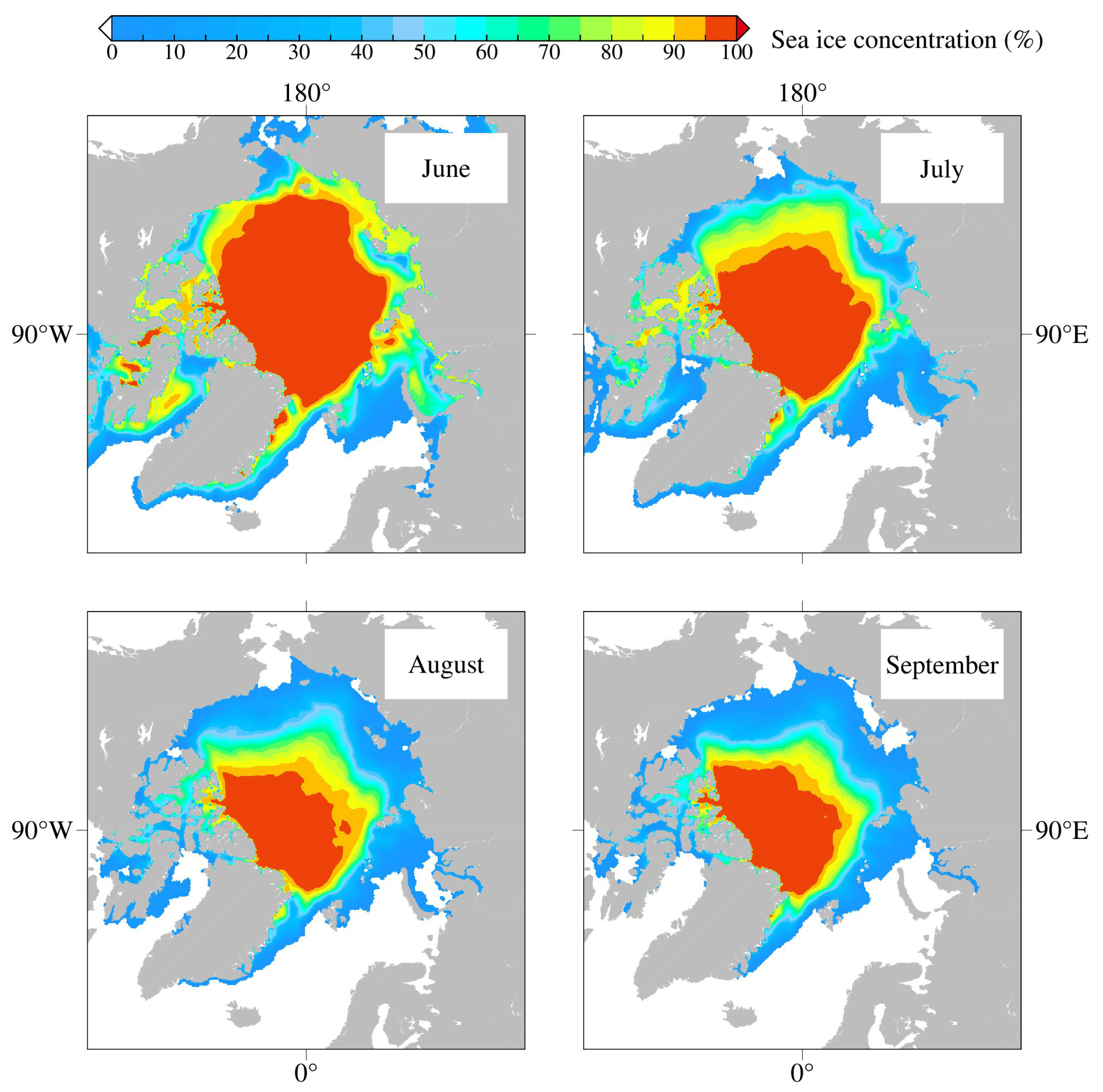
As Figure 2 shows, over the initial two decades of the 21st century, the spatial distribution of sea ice concentration (SIC) from June to September varies significantly in the coastal regions of the Arctic. In June, the NEP is almost entirely covered by sea ice, except for a few regions in the Laptev Sea and the Kara Sea where SIC falls below 50%. Arctic sea ice undergoes rapid changes from June to September. The regions with rapid changes are primarily located in the northern of the Chukchi Sea, the East Siberian Sea, certain parts of the Laptev Sea, and the northern part of the Kara Sea. Among these, the areas showing the most significant variations are primarily found in the northern Chukchi Sea and the East Siberian Sea, where the overall regional differences exceed 80%, reaching as high as 95%. In comparison, other maritime areas exhibit relatively minor fluctuations in SIC, with differences below 50%, and some regions show changes of up to 70%. It is noteworthy that in September, the northeastern of Greenland exhibited SIC approximately 14% higher than those recorded in June. The central Arctic consistently maintained near-100% sea ice coverage over the 20 years, with monthly variations remaining below 1%. Furthermore, the Barents Sea remains virtually ice-free throughout the year.

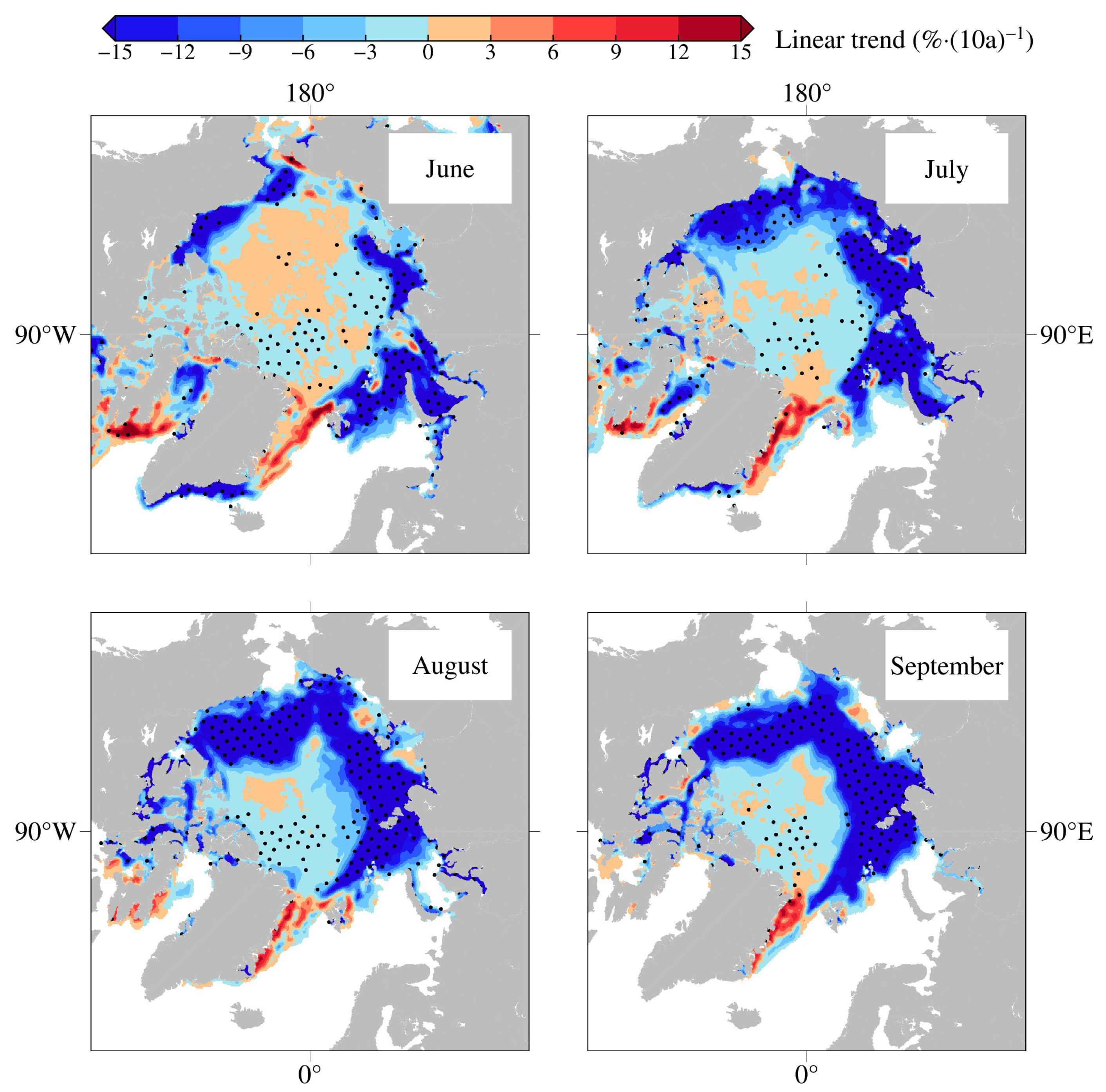
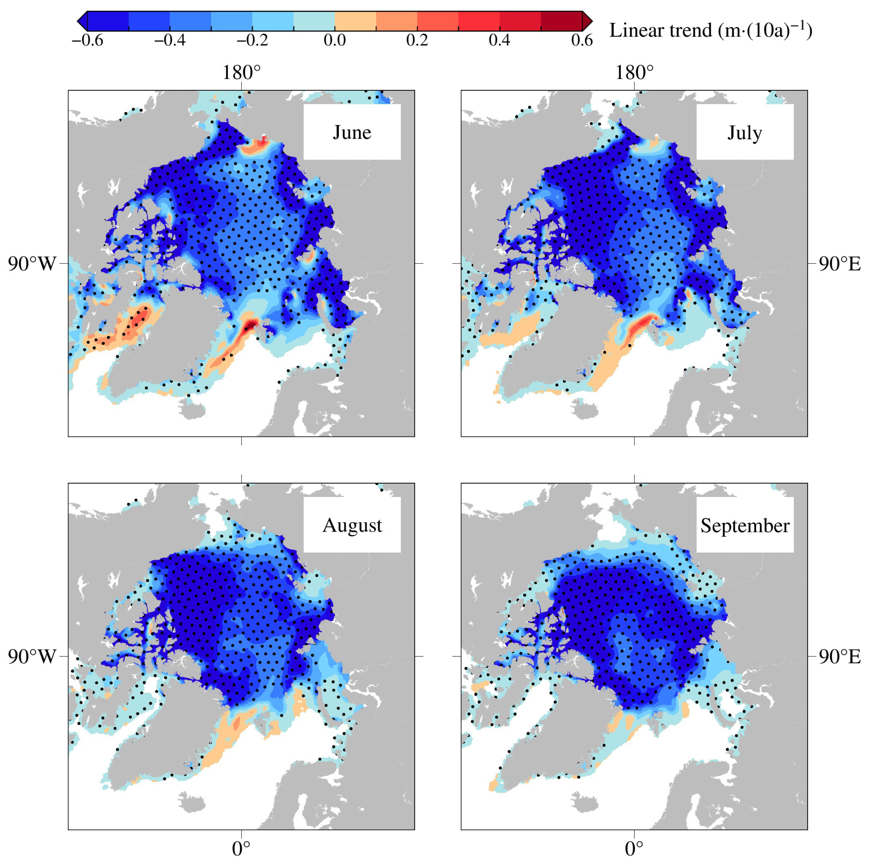
Figure 3 shows that a declining trend of SIC predominates in most regions of the Arctic over the two decades. The most notable region of SIC declining is evident along the coastlines and progressively extends the central Arctic from June to September. In particular, coastal regions experience significant reductions in SIC as the trend shifts northward from June through September. In comparison, SIC in the central Arctic is high all year-round, showing negligible monthly variations and long-term changes, which is relatively pale in comparison to the pronounced shifts seen in coastal areas. Additionally, there is a subtle uptrend in the northeastern direction from Greenland during June, July, and September.

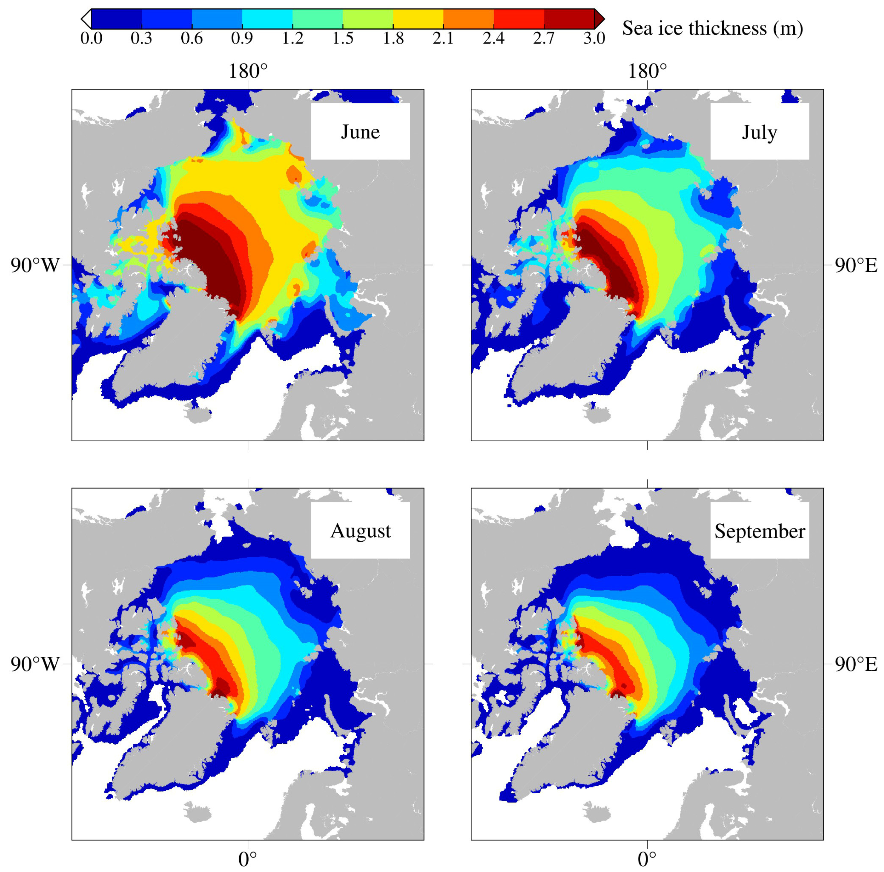
The spatial distribution of sea ice thickness (SIT) shares many characteristics with SIC, as shown in Figure 4. In the first two decades of the 21st century, the Arctic region featured notably high SIT, with areas that experience rapid monthly changes primarily located along the coastlines. In June, the SIT in most parts of the NEP exceeded 1.6 m. Particularly to the east of the Drang Strait and the Sonikov Strait, SIT even exceeded 2 m. However, specific areas of the Laptev and Kara Seas saw SIT below 1.2 m. Among them, the areas with the most significant variation in SIT between June and September were distributed in the northern regions of the East Siberian Sea and the Chukchi Sea, with differences beyond 1.7 m in most areas, especially those like the east of the Drang Strait and the Sonikov Strait, showing disparities over 2 m, which is similar to the central Arctic. Unlike SIC, the central Arctic recorded noteworthy variations in SIT, with a decrease of around 0.8 m from June to September.

An examination of the spatial distribution of SIT trends over two decades, as presented in Figure 5, reveals a declining trend in SIT across most regions of the NEP. From June to August, the declining trend in SIT in the high-latitude and near North Pole routes is less obvious compared to the surrounding regions in mid-latitude and low-latitude routes. In September, there is a more rapid decrease in SIT in areas distant from the continent. Furthermore, the trend of decreasing SIT in the eastern part of the Kara Sea is consistently less significant over the course of four months compared to the surrounding areas. A notable exception exists in some areas east of Greenland, which see an uptick in June and July.

3.1.2. Distribution and Variation of Sea Fog Frequency

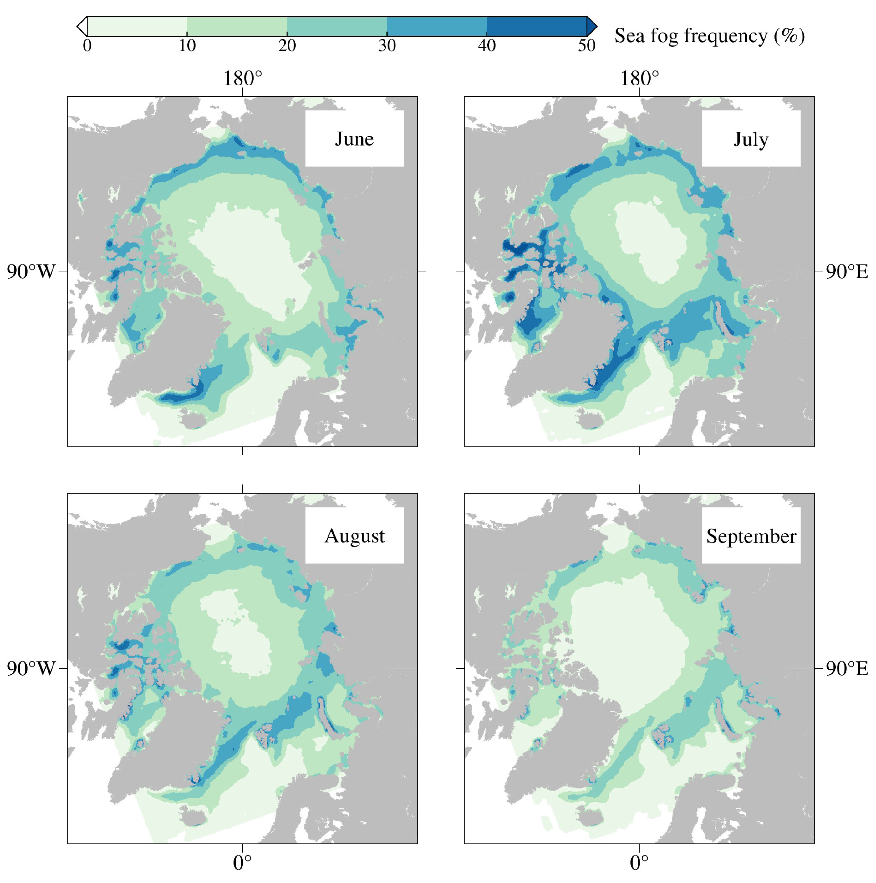
The spatial distribution of the multi-year average of Arctic sea fog frequency (SFF) from June to September exhibits an interesting contrast with the distribution of SIC and SIT (Figure 6). Higher SFF are primarily observed along the coastal regions, with a decrease in SFF as latitude increases. Notably, from June to July, the SFF remains consistently above 20% in coastal regions. Compared to the other three months mentioned above, September records the lowest SFF. Combined with the spatial distribution of sea ice, it becomes evident that September is the most suitable month for navigation during the period from 2001 to 2020. SFF in the central Arctic consistently maintains levels below 10%.

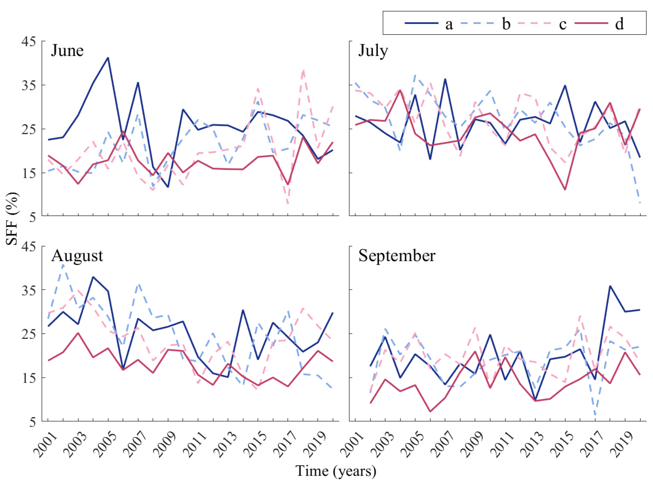
The SFF in four regions did not exhibit a significant trend over the course of 20 years (Figure 7). In September, sea fog has the least impact on navigation in the NEP, and among the four regions, the Barents Sea offers more favorable sailing conditions. When comparing the multi-year average of SFF across different months (

Table 1. Multi-year mean SFF in four regions from June to September: (a) East Siberian Sea, (b) Laptev Sea, (c) Kara Sea, and (d) Barents Sea.

	Region a	Region b	Region c	Region d	Mean
June	25.57%	21.38%	19.92%	17.53%	21.1%
July	26.07%	27.03%	27.28%	24.48%	26.22%
August	25.38%	24.78%	23.95%	18.03%	23.04%
September	20.19%	18.89%	19.56%	13.88%	18.19%
Mean	24.30%	23.02%	22.73%	18.48%	22.13%

), it is evident that July has the highest SFF, with all four regions exceeding 24%. Conversely, September exhibits the lowest SFF, with a mean falling below 20%. In terms of regional comparisons, the Barents Sea has the smallest multi-year average of SFF at 18.5%, while the other three regions have SFF values of 24.3% for the East Siberian Sea, 23% for the Laptev Sea, and 22.7% for the Kara Sea.

3.2. The Impact of Sea Fog on Route Planning

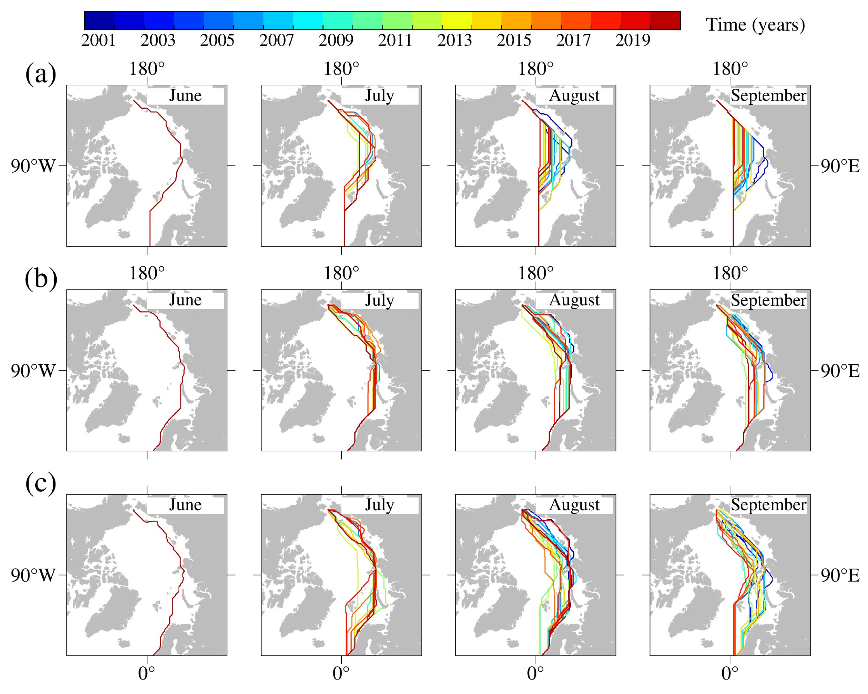
Figure 8 illustrates the route distribution of a PC6 in the NEP from June to September over the first two decades of this century. It includes the shortest route, the fastest route considering sea ice, and the new fastest route considering both sea ice and sea fog. In terms of navigational probability, the highest likelihood of navigation is observed in August and September, while June presents the lowest likelihood. Specifically, August and September were navigable for 18 years each, July was navigable 12 years, and June was navigable only in the year 2020.

In terms of route distribution, the three routes exhibit distinctive characteristics. The shortest route occupies the highest latitudes, originating from the Bering Strait, traversing the Chukchi Sea, East Siberian Sea, and the Laptev Sea, and passing through the northern regions of the Kara Sea and the Barents Sea. Over the course of 20 years, there is a noticeable trend of the route migrating towards higher latitudes. The fastest route has the lowest distribution latitude, and its course is closer to the Russian coastline. In comparison to the shortest route, this route takes a longer path through the northern regions of the Kara Sea and the Barents Sea. However, due to lower SIC and SIT, vessels can complete the navigation in a shorter duration. When further considering the impact of sea fog on sailing speed, the latitude of the new fastest routes, which incorporate both sea ice and sea fog deceleration effects, falls between that of the original fastest route and the shortest route.

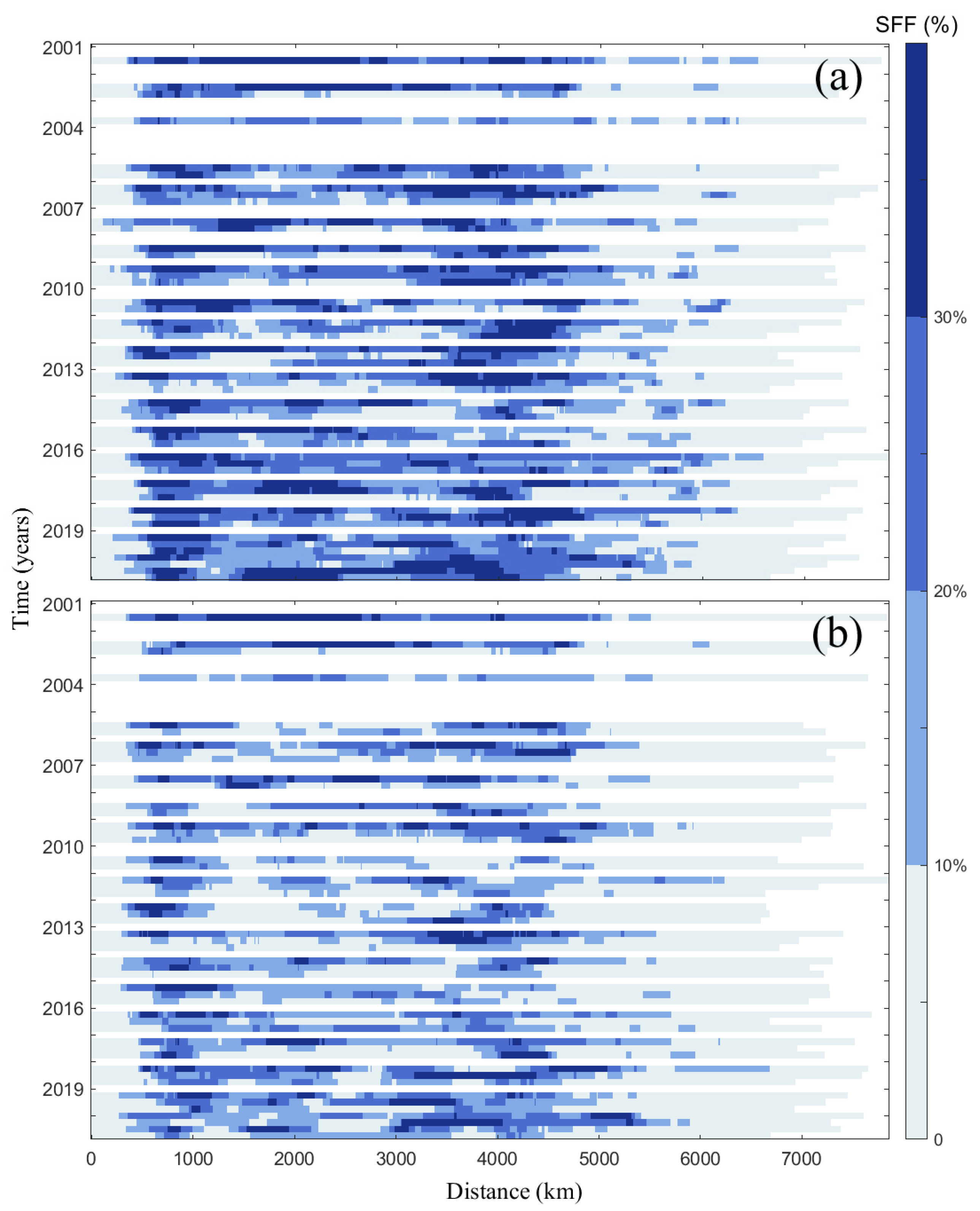
In this study, we compared the changes in SFF along the original fastest route and the new fastest route, based on the cumulative sailing distances starting from the Bering Strait. As shown in Figure 9, it is evident that the SFF along the new fastest route is significantly lower compared to the original fastest route. During 2001–2020, for the original fastest route, the mean distance affected by sea fog-induced deceleration (SFF > 10%) is approximately 4280 km, accounting for 53.3% of the total sailing distance (

Table 2. The annual mean percentage of sailing distance affected by sea fog relative to total distance. Route I is the original fastest route considering sea ice. Route IF is the new fastest route considering both sea ice and sea fog.

Year	Route I	Route IF	Year	Route I	Route IF
2001	66.31%	58.26%	2011	51.03%	38.35%
2002	40.93%	37.33%	2012	47.28%	27.98%
2003	60.22%	50.00%	2013	45.34%	36.54%
2004	/	/	2014	47.61%	36.45%
2005	53.80%	35.82%	2015	49.09%	35.38%
2006	52.26%	45.35%	2016	68.22%	47.95%
2007	51.36%	38.09%	2017	48.32%	35.99%
2008	42.86%	33.84%	2018	60.90%	49.67%
2009	57.06%	47.54%	2019	57.19%	45.93%
2010	52.18%	27.63%	2020	60.74%	47.67%

). The maximum distance affected by sea fog-induced deceleration can reach 6210 km, representing 72.3% of the total monthly route distance. The average distance of routes with high SFF (SFF > 30%) amounts to 1080 km. In contrast, the new fastest route experiences a reduced average distance affected by sea fog-induced deceleration, totaling 3270 km, which accounts for 40.8% of the total distance. The maximum distance affected by sea fog-induced deceleration on this route reaches 5310 km, representing 65.2% of the monthly route. The average distance for routes with high SFF decreases to 420 km, constituting only 38.9% of the original fastest route. The reason for this is that the SFF along the Russian coastline is higher, leading to a more pronounced deceleration effect on vessels and a substantial increase in sailing time. Consequently, the new fastest route tends to be concentrated in regions of higher latitude with lower SFF.

3.3. The Impact of Sea Fog on Navigational Efficiency

We quantified the navigational efficiency of three routes, analyzing sailing time, sailing distance, and average sailing speed for navigation (Figure 10). To emphasize the impact of sea fog on navigational efficiency, we divided the original fastest route into two scenarios: one considering sea ice only and the other incorporating the impacts of sea fog.

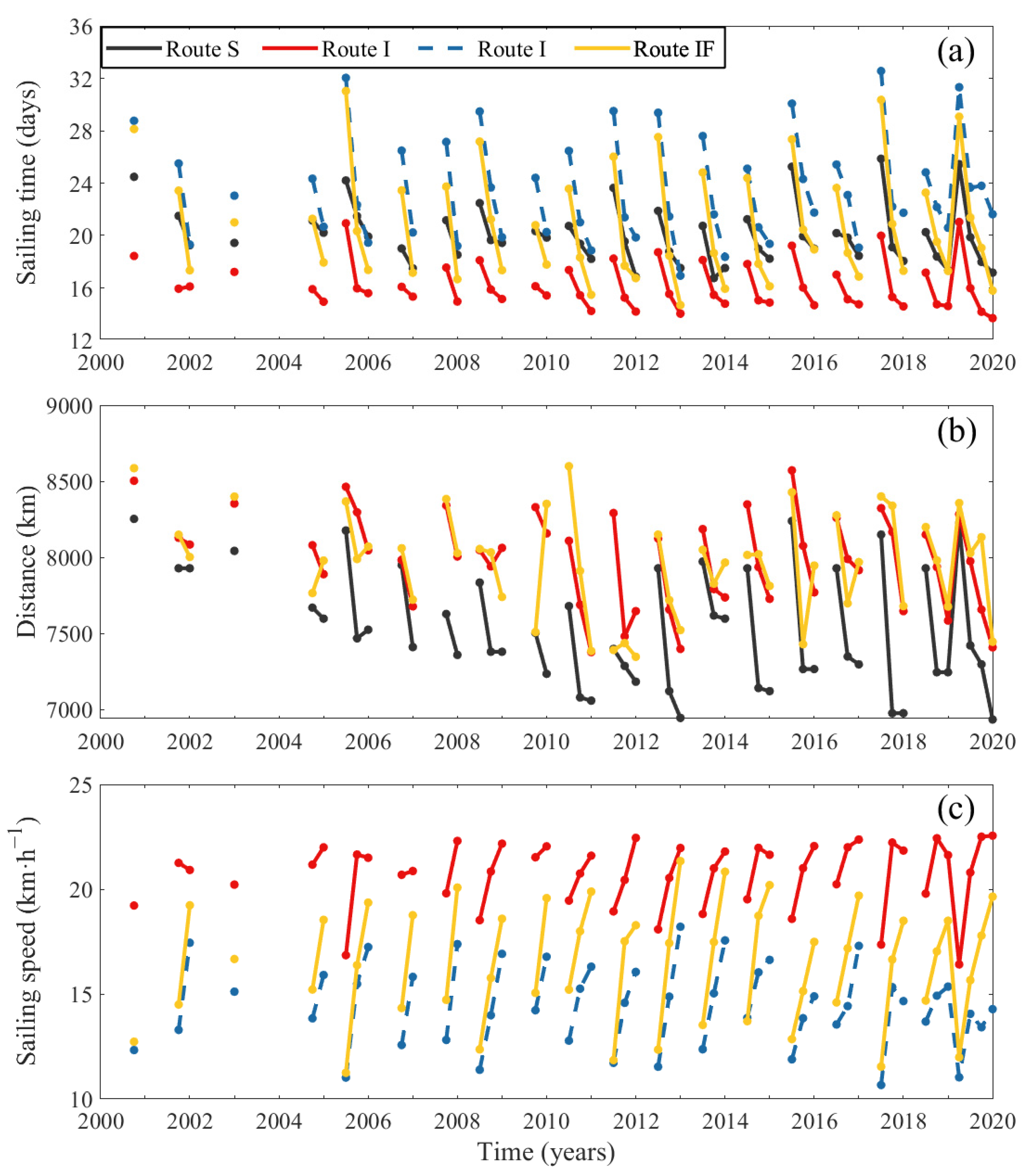
When considering sea ice alone, the shortest route and the fastest route each have their advantages. During the period from 2001 to 2020, the average distance covered by vessels following the shortest route was approximately 7530 km, with an average sailing duration of 20 days. In contrast, vessels following the fastest route covered a distance of 7992 km on average, with an average sailing duration of 16.2 days. Compared to the shortest route, the fastest route in the same month had an increasing sailing distance ranging from 150 to 920 km, while the sailing time decreased by 1.3 to 6 days. Due to the influence of sea ice, the routes in the Arctic vary seasonally based on ice conditions, and the shortest and fastest routes are not always the same. Vessels should consider factors such as fuel or cargo loss when choosing the most suitable route in a cost-effective manner.

The impact of Arctic sea fog on navigational efficiency is significant. When comparing the optimized new fastest route considering both sea ice and sea fog to the original fastest route considering sea fog deceleration, there is a noticeable improvement in navigational efficiency. If vessels were to encounter deceleration due to Arctic sea fog on the original fastest route, their average sailing speed would decrease by 30.2%, resulting in an average sailing time of 23.5 days., In contrast, the sea fog led to an increase of 45.1% in sailing time. This substantially diminishes the navigational efficiency of vessels in the NEP. In contrast, vessels following the optimized new fastest route considering both sea ice and sea fog complete the journey with an average total distance of approximately 7966 km and an average sailing time of approximately 20.8 days. While the new fastest route covers a distance similar to that of the original fastest route, the optimized new fastest route exhibits a 13.9% increase in average sailing speed and an 11.5% reduction in sailing time compared to the original fastest route. These optimization results significantly enhance navigational efficiency.

4. Discussion

Previous studies on route planning in the NEP have mostly relied on the calculation of the least-cost route accumulating the lowest total time or distance based on sea ice data only. Given the unique characteristics of the NEP in contrast to other oceans, sea ice not only limits where ships can go but also affects their speed in navigable areas. The shortest route is not always the fastest, so vessels should weigh factors like fuel and cargo expenses when deciding between the shortest and fastest routes. In terms of the shortest route, the sailing time was reported as approximately 17 days during the summer of the 2020s in a previous study, while our research indicates a longer duration of 20 days in the first two decades of the 21st century [4]. Concerning the fastest route, Melia et al. proposed a sailing time of approximately 19 days from Yokohama to Rotterdam during the period from 2015 to 2029 [22], and the result in this study shows a mean sailing time of 16 days from the Bering Strait to Rotterdam. Considering the sailing time from Yokohama to the Bering Strait, the difference between these two results is about 2 days. Furthermore, the previous studies suggested the potential opening of the Central Passage for a PC6 as early as after 2030 [22,32,33]. However, this study reveals that the Central Passage had already become accessible for the PC6 by 2020, which is similar with the findings of Cao et al. [9].

From the detailed analysis provided, it is clear that when sea fog is considered, the NEP’s outcomes differ significantly from when only sea ice is factored in, both for route planning and navigational efficiency. Using the POLARIS to plan Arctic shipping routes aids in understanding the future potential of Arctic navigation. Furthermore, incorporating sea fog’s effects enhances the navigation model’s practical applicability.

Additionally, given the influence of sea fog on sailing speed and safety, depending solely on the original fastest route, which only considers sea ice, might not be the best option. In addition, compared with the number of foggy days, the range of visibility also has an important impact on the ship speed. However, there are little extensive and continuously observed sea fog data in the NEP, as well as insufficient reliable information for quantifying the effects of sea fog on safe speeds. This limitation makes it challenging to support safe navigation in the NEP with timely and dependable sea fog data, hampering progress in research related to the NEP and Arctic sea fog. Currently, models play an essential role in offering continuous spatiotemporal insights into sea fog. The SFF data in this study are derived from daily average visibility data, which are generated by models. Although these data might not suit shorter time-scale studies, like daily or hourly analysis, and cannot be employed for real-time navigation and safety services, the route optimization findings suggest that future ship navigation and simulations should consider a broader range of influencing factors to be more comprehensive and reasonable.

The POLARIS, as a cutting-edge tool for quantifying navigation risks, encompasses a wide variety of vessel types and offers detailed segmentation of sea ice thickness. This makes it integral to contemporary Arctic route planning research. However, it does not account for real-time factors like ice conditions, weather, or sea state, among other natural variables. Furthermore, it does not factor in human-induced elements like the quality of coastal navigation infrastructure or regional navigation policies. By solely relying on data about ship icebreaking capabilities and sea ice thickness and concentration, the resulting composite navigation risk index might not adequately capture the maritime area’s navigational conditions. This study’s results highlight the variability in maritime route choices, which are contingent on several factors, including whether the shortest or fastest route is selected. Even within the same route category, factoring in diverse navigational influences can lead to different planning results. As the NEP increasingly becomes accessible, the future will likely emphasize a holistic approach, taking into account various natural factors such as sea ice, oceanic conditions, and weather patterns. The emphasis on delivering real-time navigation safety services in the Arctic, drawing on updated data on sea ice, ocean conditions, and meteorology, will become a crucial direction for development.

5. Conclusions

Arctic sea fog is a major factor influencing vessel safety and navigational efficiency in the NEP. Presently, much of the research centers on the effects of sea ice in determining the least-cost route, which accumulates the minimum time or distance. In our study, we examined the combined effects of sea ice and sea fog on route planning and navigation efficiency within the NEP. Using the POLARIS model, we quantified navigation risks for a PC6 in the NEP from June to September across the initial two decades of the 21st century. Our analysis encompasses route planning and navigational efficiency, including the shortest route, the fastest route considering sea ice, and the new fastest route considering both sea ice and sea fog.

From 2001 to 2020, the NEP consistently had sea ice coverage. Yet, the coastal areas along the continent have less extensive sea ice compared to the central Arctic, showing pronounced monthly variations. Additionally, most of this region observed a decreasing trend in sea ice concentration and thickness over the two decades. Contrasting with sea ice distribution, regions with elevated SFF are predominantly found along the Arctic’s coastal areas, with a decline as latitude rises. Among the four months, September has the most minimal sea ice and the lowest SFF in the NEP, translating to the highest navigational probability.

In navigation outcomes and focusing solely on sea ice’s influence, the shortest route has an average sailing duration of 20 days, with a clear trend towards higher latitudes over the two decades. In contrast, the fastest route reduces the average sailing duration by about 4 days, and the distribution of this route aligns closer to the Russian coast. When factoring in sea fog, the average speed for the original fastest route drops by 30.2%, extending the average sailing duration to 25.3 days.

The new fastest route, which considered both sea ice and sea fog, sits between the latitudes of the shortest and the original fastest routes. Relative to the original fastest route, the new fastest route has a lower SFF, which considerably lessens the distance influenced by sea fog. The new route, though covering a distance akin to the original’s, sees a 13.9% uptick in average speed and shaves off 11.5% of the sailing duration, markedly boosting navigational efficiency.

The results in our study indicate that relying solely on sea ice as a predictive factor does not provide a convincing forecast for future vessel navigation in the NEP. There is a note that the results of this study are focused on the first two decades in the 21st century; the long-term projection of NEP route planning should be further analyzed. It is imperative to incorporate additional variables to make navigation model more comprehensive and reliable. Meanwhile, visibility directly affects the speed of vessels in the NEP, while monthly SFF data can only roughly reflect the deceleration effect of sea fog on ships. The Arctic navigation model can be optimized based on daily or hourly extensive and continuous observed visibility data and sea ice data to serve risk simulation or ship navigation in the future.

References

- Serreze, M.C.; Meier, W.N. The Arctic’s sea ice cover: Trends, variability, predictability, and comparisons to the Antarctic. Ann. N. Y. Acad. Sci. 2019, 1436, 36–53. [Google Scholar] [CrossRef] [PubMed]
- Kwok, R. Arctic sea ice thickness, volume, and multiyear ice coverage: Losses and coupled variability (1958–2018). Environ. Res. Lett. 2018, 13, 105005. [Google Scholar] [CrossRef]
- Notz, D.; SIMIP Community. Arctic Sea Ice in CMIP6. Geophys. Res. Lett. 2020, 47, e2019GL086749. [Google Scholar] [CrossRef]
- Min, C.; Yang, Q.; Chen, D.; Yang, Y.; Zhou, X.; Shu, Q.; Liu, J. The Emerging Arctic Shipping Corridors. Geophys. Res. Lett. 2022, 49, e2022GL099157. [Google Scholar] [CrossRef]
- Biskaborn, B.K.; Smith, S.L.; Noetzli, J.; Matthes, H.; Vieira, G.; Streletskiy, D.A.; Schoeneich, P.; Romanovsky, V.E.; Lewkowicz, A.G.; Abramov, A.; et al. Permafrost is warming at a global scale. Nat. Commun. 2019, 10, 264. [Google Scholar] [CrossRef]
- Box, J.E.; Colgan, W.T.; Christensen, T.R.; Schmidt, N.M.; Lund, M.; Parmentier, F.J.W.; Brown, R.; Bhatt, U.S.; Euskirchen, E.S.; Romanovsky, V.E.; et al. Key indicators of Arctic climate change: 1971–2017. Environ. Res. Lett. 2019, 14, 045010. [Google Scholar] [CrossRef]
- Loomis, B.D.; Rachlin, K.E.; Luthcke, S.B. Improved Earth Oblateness Rate Reveals Increased Ice Sheet Losses and Mass-Driven Sea Level Rise. Geophys. Res. Lett. 2019, 46, 6910–6917. [Google Scholar] [CrossRef]
- Stroeve, J.; Notz, D. Changing state of Arctic sea ice across all seasons. Environ. Res. Lett. 2018, 13, 103001. [Google Scholar] [CrossRef]
- Cao, Y.; Liang, S.; Sun, L.; Liu, J.; Cheng, X.; Wang, D.; Chen, Y.; Yu, M.; Feng, K. Trans-Arctic shipping routes expanding faster than the model projections. Glob. Environ. Chang. 2022, 73, 102488. [Google Scholar] [CrossRef]
- Gunnarsson, B.; Moe, A. Ten years of international shipping on the Northern Sea Route: Trends and challenges. Arct. Rev. Law Politics 2021, 12, 4–30. [Google Scholar] [CrossRef]
- Buixadé Farré, A.; Stephenson, S.R.; Chen, L.; Czub, M.; Dai, Y.; Demchev, D.; Efimov, Y.; Graczyk, P.; Grythe, H.; Keil, K.; et al. Commercial Arctic shipping through the Northeast Passage: Routes, resources, governance, technology, and infrastructure. Polar Geogr. 2014, 37, 298–324. [Google Scholar] [CrossRef]
- Schøyen, H.; Bråthen, S. The Northern Sea Route versus the Suez Canal: Cases from bulk shipping. J. Transp. Geogr. 2011, 19, 977–983. [Google Scholar] [CrossRef]
- Lasserre, F. Case studies of shipping along Arctic routes. Analysis and profitability perspectives for the container sector. Transp. Res. Part A Policy Pract. 2014, 66, 144–161. [Google Scholar] [CrossRef]
- Marchenko, N. Russian Arctic Seas: Navigational Conditions and Accidents; Springer Science & Business Media: Berlin/Heidelberg, Germany, 2012. [Google Scholar] [CrossRef]
- Mulherin, N.D. The Northern Sea Route: Its Development and Evolving State of Operations in the 1990s; CRREL: Hanover, NH, USA, 1996. [Google Scholar]
- Li, X.; Lynch, A.H. New insights into projected Arctic sea road: Operational risks, economic values, and policy implications. Clim. Chang. 2023, 176, 30. [Google Scholar] [CrossRef] [PubMed]
- Chen, J.; Kang, S.; Du, W.; Guo, J.; Xu, M.; Zhang, Y.; Zhong, X.; Zhang, W.; Chen, J. Perspectives on future sea ice and navigability in the Arctic. Cryosphere 2021, 15, 5473–5482. [Google Scholar] [CrossRef]
- Chen, J.; Kang, S.; You, Q.; Zhang, Y.; Du, W. Projected changes in sea ice and the navigability of the Arctic Passages under global warming of 2 °C and 3 °C. Anthropocene 2022, 40, 100349. [Google Scholar] [CrossRef]
- Chen, J.; Kang, S.; Chen, C.; You, Q.; Du, W.; Xu, M.; Zhong, X.; Zhang, W.; Chen, J. Changes in sea ice and future accessibility along the Arctic Northeast Passage. Glob. Planet. Chang. 2020, 195, 103319. [Google Scholar] [CrossRef]
- Li, X.; Stephenson, S.R.; Lynch, A.H.; Goldstein, M.A.; Bailey, D.A.; Veland, S. Arctic shipping guidance from the CMIP6 ensemble on operational and infrastructural timescales. Clim. Chang. 2021, 167, 23. [Google Scholar] [CrossRef]
- Wei, T.; Yan, Q.; Qi, W.; Ding, M.; Wang, C. Projections of Arctic sea ice conditions and shipping routes in the twenty-first century using CMIP6 forcing scenarios. Environ. Res. Lett. 2020, 15, 104079. [Google Scholar] [CrossRef]
- Melia, N.; Haines, K.; Hawkins, E. Sea ice decline and 21st century trans-Arctic shipping routes. Geophys. Res. Lett. 2016, 43, 9720–9728. [Google Scholar] [CrossRef]
- Nam, J.H.; Park, I.; Lee, H.J.; Kwon, M.O.; Choi, K.; Seo, Y.K. Simulation of optimal arctic routes using a numerical sea ice model based on an ice-coupled ocean circulation method. Int. J. Nav. Archit. Ocean. Eng. 2013, 5, 210–226. [Google Scholar] [CrossRef]
- Song, S.; Chen, Y.; Chen, X.; Chen, C.; Li, K.F.; Tung, K.K.; Shao, Q.; Liu, Y.; Wang, X.; Yi, L.; et al. Adapting to a Foggy Future Along Trans-Arctic Shipping Routes. Geophys. Res. Lett. 2023, 50, e2022GL102395. [Google Scholar] [CrossRef]
- Comiso, J.C. Bootstrap Sea Ice Concentrations from Nimbus-7 SMMR and DMSP SSM/ISSMIS, Version 3; National Snow and Ice Data Center: Boulder, CO, USA, 2017. [Google Scholar] [CrossRef]
- Schweiger, A.; Lindsay, R.; Zhang, J.; Steele, M.; Stern, H.; Kwok, R. Uncertainty in modeled Arctic sea ice volume. J. Geophys. Res. Ocean. 2011, 116, C00D06. [Google Scholar] [CrossRef]
- Zhang, J.; Rothrock, D.A. Modeling global sea ice with a thickness and enthalpy distribution model in generalized curvilinear coordinates. Mon. Weather Rev. 2003, 131, 845–861. [Google Scholar] [CrossRef]
- Meier, W.N.; Stewart, J.S. NSIDC Land, Ocean, Coast, Ice, and Sea Ice Region Masks. NSIDC Special Report 25. Boulder CO, USA: National Snow and Ice Data Center. 2023. Available online: https://nsidc.org/sites/default/files/documents/technical-reference/nsidc-special-report-25.pdf (accessed on 14 June 2023).
- Dijkstra, E.W. A note on two problems in connexion with graphs. Numer. Math. 1959, 1, 287–290. [Google Scholar] [CrossRef]
- Aksenov, Y.; Popova, E.E.; Yool, A.; Nurser, A.G.; Williams, T.D.; Bertino, L.; Bergh, J. On the future navigability of Arctic sea routes: High-resolution projections of the Arctic Ocean and sea ice. Mar. Policy 2017, 75, 300–317. [Google Scholar] [CrossRef]
- Stephenson, S.R.; Smith, L.C.; Brigham, L.W.; Agnew, J.A. Projected 21st-century changes to Arctic marine access. Clim. Chang. 2013, 118, 885–899. [Google Scholar] [CrossRef]
- Smith, L.C.; Stephenson, S.R. New Trans-Arctic shipping routes navigable by midcentury. Proc. Natl. Acad. Sci. USA 2013, 110, E1191–E1195. [Google Scholar] [CrossRef]
- Stephenson, S.R.; Smith, L.C. Influence of climate model variability on projected Arctic shipping futures. Earth’s Future 2015, 3, 331–343. [Google Scholar] [CrossRef]
Figure 1.
Schematic diagram of the Arctic, (a) East Siberian Sea, (b) Laptev Sea, (c) Kara Sea, (d) and Barents Sea.
Figure 2.
Distribution for the multi-year average of SIC from June to September in the first two decades of the 21st century.
Figure 3.
Distribution for the linear trend of SIC from June to September in the first two decades of the 21st century. The black spots are the areas passing the 95% significance test.
Figure 4.
Distribution for the multi-year average of SIT from June to September in the first two decades of the 21st century.
Figure 5.
Distribution for the linear trend of SIT from June to September in the first two decades of the 21st century. The black spots are the areas passing the 95% significance test.
Figure 6.
Distribution for the multi-year average of SFF from June to September in the first two decades of the 21st century.
Figure 7.
Annual mean SFF in four regions from June to September in the first two decades of the 21st century: (a) East Siberian Sea, (b) Laptev Sea, (c) Kara Sea, and (d) Barents Sea.
Figure 8.
Shipping routes distribution from June to September in the first two decades of the 21st century: (a) the shortest route, (b) the fastest route considering sea ice, (c) and the new fastest route considering both sea ice and sea fog.
Figure 9.
The SFF along the shipping routes: (a) the original fastest route considering sea ice, and (b) the new fastest route considering both sea ice and sea fog.
Figure 10.
The (a) sailing time, (b) distance, and (c) sailing speed among the shipping routes. Route S is the shortest route. Route I is the fastest route considering sea ice. The blue dashed line is also Route I while calculating the deceleration of sea fog. Route IF is the new fastest route considering both sea ice and sea fog.