Article

Forecasting Vertical Profiles of Ocean Currents from Surface Characteristics: A Multivariate Multi-Head Convolutional Neural Network–Long Short-Term Memory Approach

Roger F. Wicker Center for Ocean Enterprise, The University of Southern Mississippi, Gulfport, MS 39501, USA
*
Author to whom correspondence should be addressed.
J. Mar. Sci. Eng. 2023, 11(10), 1964; https://doi.org/10.3390/jmse11101964
Submission received: 6 September 2023 / Revised: 5 October 2023 / Accepted: 9 October 2023 / Published: 11 October 2023

Abstract

:
While study of ocean dynamics usually involves modeling deep ocean variables, monitoring and accurate forecasting of nearshore environments is also critical. However, sensor observations often contain artifacts like long stretches of missing data and noise, typically after an extreme event occurrence or some accidental damage to the sensors. Such data artifacts, if not handled diligently prior to modeling, can significantly impact the reliability of any further predictive analysis. Therefore, we present a framework that integrates data reconstruction of key sea state variables and multi-step-ahead forecasting of current speed from the reconstructed time series for 19 depth levels simultaneously. Using multivariate chained regressions, the reconstruction algorithm rigorously tests from an ensemble of tree-based models (fed only with surface characteristics) to impute gaps in the vertical profiles of the sea state variables down to 20 m deep. Subsequently, a deep encoder–decoder model, comprising multi-head convolutional networks, extracts high-level features from each depth level’s multivariate (reconstructed) input and feeds them to a deep long short-term memory network for 24 h ahead forecasts of current speed profiles. In this work, we utilized Viking buoy data, and demonstrated that with limited training data, we could explain an overall 80% variation in the current speed profiles across the forecast period and the depth levels.

1. Introduction

Understanding and effective modeling of the dynamics in marine (coastal and open ocean/deep sea) ecosystems are critical to scientific research and ecosystem analysis. One of the significant applications of ocean modeling is the long-term weather forecasting associated with El Niño, which requires substantial historical data on the physical characteristics of the oceans [1,2]. However, for short-term forecasts like predicting the currents or changes in water density in estuaries or nearshore regions, detailed measurement of surface/subsurface variables is required. Apart from scientific implications, blue research also supports the data collection and information mining necessary for the development of a new blue economy, which is focused on revitalizing the marine industrial activities. These activities encompass ship building, communication cable laying, equipment deployment, sustainable energy from waves, currents, seaside leisure tourism, fisheries, and aquaculture, etc. [3]. Therefore, ocean observation data are being increasingly utilized for developing intelligent solutions that can track, predict, manage, and adapt to changes in the marine environment, in real or near-real time [4,5].
Ocean observation data typically span five types: physical data, biological data, chemical data, geological data, and socioeconomic data [6], commonly measured using buoys, water column samplers, and floats. Using several platforms, like unmanned marine vehicles, research vessels, etc., collaborative research efforts are directed towards democratizing these datasets. The commonly used open-source ocean data sources are the National Centers for Environmental Information (NCEI), National Data Buoy Center (NDBC), Integrated Ocean Observing Systems (IOOS), etc., in addition to the Gulf of Mexico Coastal Ocean Observing System (GCOOS) and the Coastal CUBEnet, focused on providing Gulf of Mexico (GoM)-specific data [7]. While these data sources house unfathomable volumes and a variety of ocean observation data, efficient utilization of these datasets and the development of sustainable data-driven solutions are impeded by a range of artifacts in the raw data. The commonly noticed data artifacts are long contiguous and/or intermittent gaps and noise present in the time series of the observed variables. Such a lack of complete observation data mostly occurs from sensor malfunction during extreme wave conditions, especially if the sensors are deployed in the coastal or shallower regions [8,9].
Here, we have attempted to address the artifact of missingness in ocean observation data and provide a data-driven solution for the systematic utilization of the reconstructed time series of multiple physical sea state variables, through a deep learning pipeline that can potentially aid intelligent ocean readiness. To demonstrate the workflow, we have leveraged the University of Southern Mississippi’s (USM) Viking buoy (WMO-42067) data, moored 20 m below the sea surface in the nearshore regions of the northern GoM. The sensors integrated in the buoy measured several meteorological and oceanographic variables, and in this case study, we have first focused on the reconstruction of the vertical profiles of water temperature (WTMP), salinity (SAL), and current speed (CS) from the surface characteristics. And the second module of the pipeline involved a deep learning model, developed from the reconstructed attributes to provide simultaneous one-day-ahead forecasts of the CS for various depths in the water column. Notably, reliable current monitoring is an important consideration in offshore and coastal design [10,11].
Temperature and salinity gradients are some of the significant drivers that shape the ocean currents, which are critical to marine ecosystems since they redistribute heat, water, nutrients, and oxygen in the ocean [12]. Temperature differences across the globe influence global wind patterns, which, in turn, impact ocean currents. Such differences also drive a vital component of ocean circulation known as thermohaline circulation, where ‘thermo’ refers to temperature, and ‘haline’, salinity [13]. Cold and salty water, being denser than the warm and less salty water, sinks and flows along the ocean floor, forming deep ocean currents. Eventually, these deep currents can rise to the surface in different parts of the world, completing the circulation loop [14].
The salinity gradients, on the other hand, can create a layer of rapidly changing salinity, known as a halocline, that acts as a barrier, impeding the vertical mixing of water masses and influencing the movement of ocean currents [13]. The presence of a halocline can cause the upper and lower layers of water to move independently, leading to the development of different current systems. Effectively, salinity also affects the density of seawater. Higher salinity increases water density, making it denser and more prone to sinking. Near the coastlines, salinity variations between the coastal water and the open ocean influence the development of coastal currents, consequently affecting the near-surface marine ecosystems [15]. These implications are not only critical from a marine science perspective, but also majorly impact the ballasting designs of the undersea vehicles, since it is critical to ensure that an underwater vehicle can remain neutrally buoyant through varying depths [16]. Therefore, predictive analysis of currents is largely associated with simultaneous modeling of the temperature and salinity profiles, in addition to other environmental variables.
Traditionally, numerical ocean circulation models (based on physical schemes defined by certain governing equations) are utilized for predicting vertical profiles of ocean subsurface temperature, salinity, and current [17]. Ocean models widely used in physical oceanography include the Regional Ocean Modeling System (ROMS) [18], Modular Ocean Model (MOM) [19], HYbrid Coordinate Ocean Model (HYCOM) [20], etc. These models are highly effective in global/regional modeling of ocean processes, and predictions of the complex air-sea interactions are achieved by coupling different numerical models into an integrated framework, e.g., the Coupled Ocean–Atmosphere–Wave–Sediment Transport (COAST) system [21]. However, their usage is limited due to very high computational and implementation complexities [22]. Therefore, for short-term predictions of physical sea state characteristics, data-driven models have recently gained momentum.
Most of the machine learning-based studies aim at reconstruction of deep ocean variables using satellite remote sensing data for spatially diverse predictions, combined with Argo float data [23,24]. For example, Han et al. [25] used satellite remote sensing observations of sea surface temperature (SST), sea surface height (SSH), and sea surface salinity (SSS) to reconstruct the monthly ocean subsurface temperature (ST) to a depth of 1800 m, using 12 discrete convolutional neural network (CNN) models. In addition to sequential networks like bi-directional long short-term memory (Bi-LSTM) models [26], other common machine learning methods used for efficient prediction of sea subsurface vertical profiles (typically down to 1000 m deep) are the Extreme Gradient Boosting method (XGBoost) [23], support vector machines [27], etc. However, many Argo floats suffer from sensor drift, resulting in large errors, varying with different locations and yet to be quantified [28]. Additionally, very few studies have measured the surface layer processes in coastal regions, although the surface layer dynamics play an important role in the momentum, heat, and energy exchanges across the air–sea interface [29].
Therefore, considering the above aspects, this study is aimed at the reconstruction of three key physical sea state characteristics (WTMP, SAL, CS) in the nearshore areas, that are only 20–30 m deep and are sites of active biogeochemical cycling. The reconstructed data are further utilized for multi-step ahead forecasting of current speeds using data-driven methods. From the literature, it has been identified that machine learning models like support vector machines or tree-based ensemble learners are usually not efficient for forecasting sea state variables at different depths and with longer lead times. Hence, deep learning approaches are typically employed, using one-dimensional convolutional layers to extract high-level features from the multivariate inputs that are passed onto sequential learners like the LSTMs for multi-step ahead predictions [30,31]. Nevertheless, such approaches mostly involve data aggregation from several individual models [25]. Therefore, to enable simultaneous, multivariate modeling of multi-level or hierarchical data spanning various depth levels, we have utilized computationally efficient chained XGBoost (interchangeably with XGB) regressors for data reconstruction. Subsequently, a single deep multi-head CNN-LSTM encoder–decoder model was leveraged for one-day-ahead CS predictions for each of the depth levels.
The data-driven models leveraged in this work allow stepwise analysis of the sea state variables, and integration of discrete modules into a complete framework for expedited forecasting of vertical current profiles from surface characteristics. For deep learning model training, although the related literature [25,26,27,30,31] commonly leverages multiple years of historical data and reports superior predictive performance, here, one of the core objectives is to test the performance of data-driven models when trained with limited data, i.e., on an experimental Viking buoy dataset, as discussed later. In summary, the major contribution of the mentioned work is the development of an end-to-end pipeline that addresses the challenges associated with data artifacts in nearshore ocean monitoring as well as forecasts current speeds at multiple depth levels simultaneously, thereby addressing the computational constraints associated with conventional numerical ocean circulation models.

2. Data and Methodology
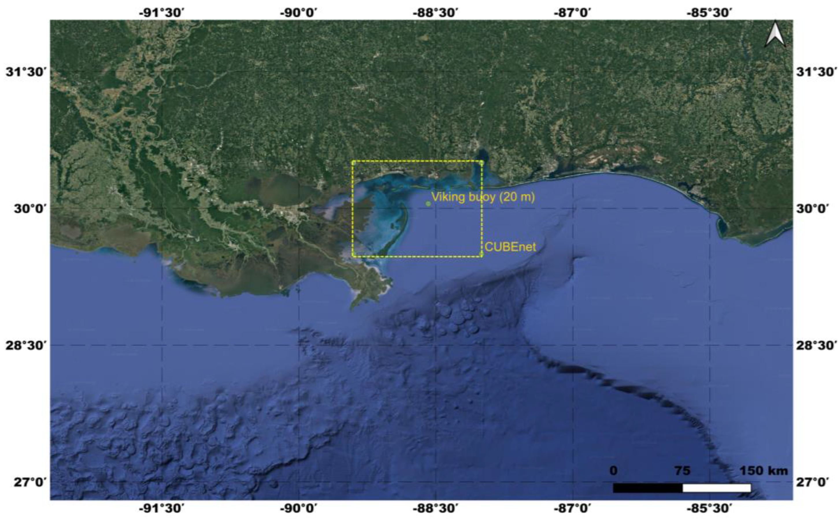
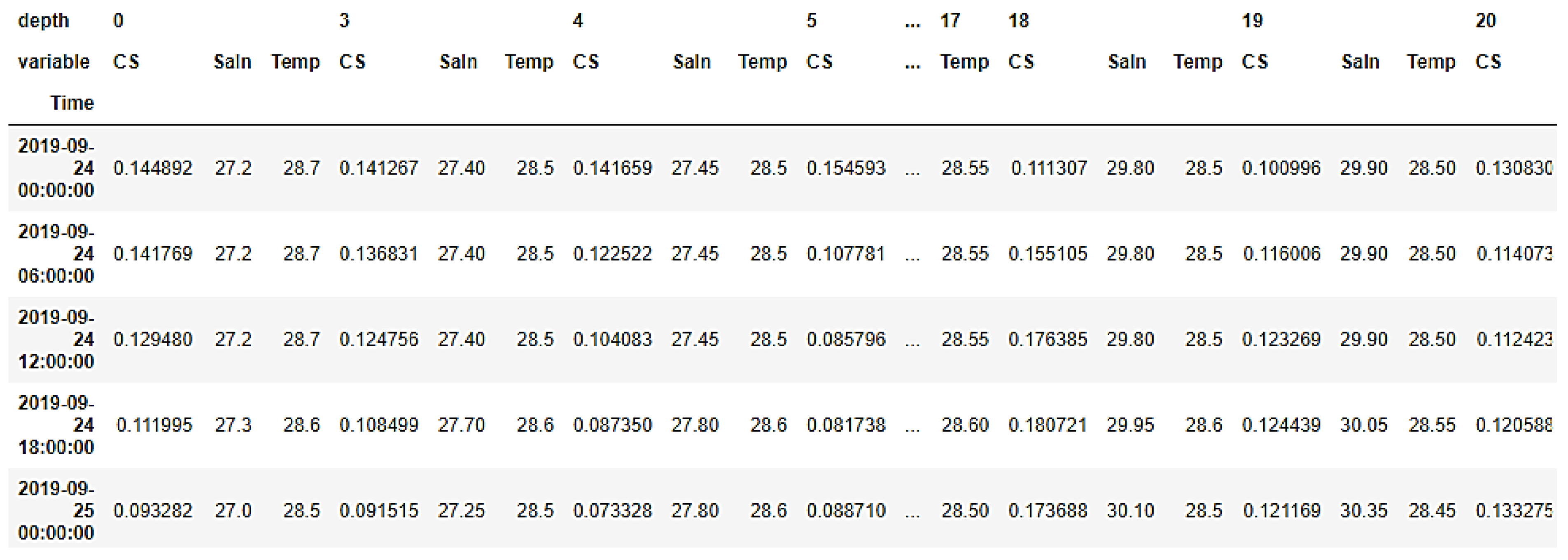
2.1. Buoy Data

The Viking buoy (USM-R1, WMO-42067) is one of the observational buoys and uncrewed systems operated by USM in the CUBEnet region [32] (Figure 1). It is a meteorological–oceanographic buoy with a diameter of 2.2 m, and it transmits data every 15 min via an Iridium satellite uplink to a server at USM. The buoy is designed to accommodate the use of many instruments, e.g., wavemeter, weather sensor, automatic CTD profiler, and the Acoustic Doppler Current Profiler (ADCP), etc., per the requirements (further details provided in Supplementary Figure S1). For this case study, the sensors on board the Viking buoy measured wave height (WVHT, m) and average wave period (APD, sec), wind direction (WDIR, °C) and wind speed (WSPD, m/s), atmospheric temperature (ATMP, °C), and pressure (PRES, hPa). Additionally, the buoy is equipped with a CTD profiler, capable of recording water temperature (WTMP, °C) and salinity (SAL, PSU) measurements at different programmable depths, and an Acoustic Doppler Current Profiler (ADCP) that records current speed (CS, m/s) at various depths throughout the water column, i.e., up to 20 m depth in this case. The period of available Viking data used in this study is from September 2019 to August 2020.

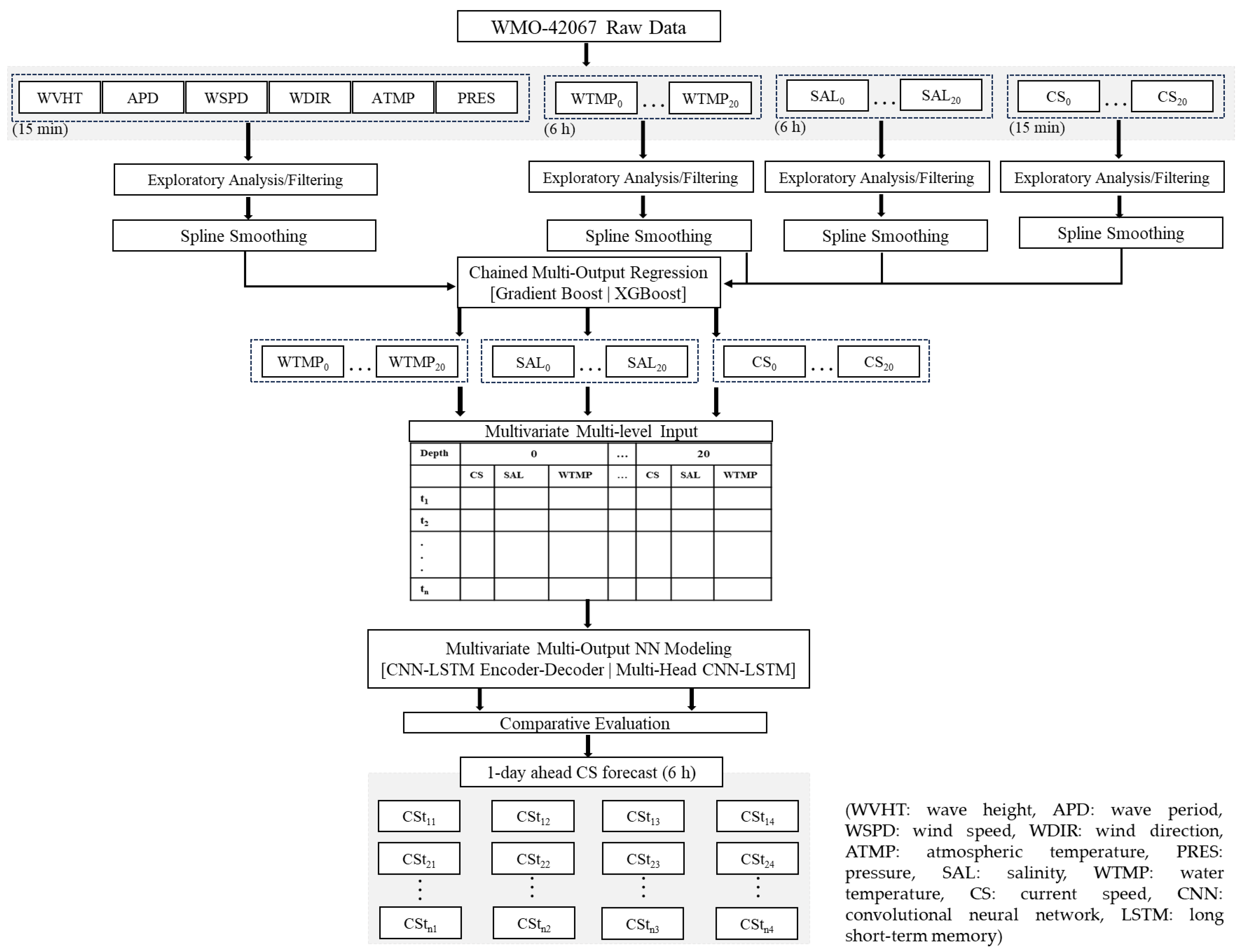
2.2. Methodology Overview

As a broader objective of this work, we aimed to test the Viking buoy data quality and its applicability to developing a forecast and alert system that could help the maritime operations with preparedness and risk mitigation. For evaluating data quality, this work focuses on extensive exploratory analysis of the raw data (Section 2.3), followed by k-fold cross-validation-based chained regression analysis for credible reconstruction of the gaps in the in situ data (Section 2.4). This ensured that the reconstructed vertical profiles of WTMP and SAL could be further utilized for simultaneous prediction of CS at different depths. Before proceeding with multi-step forecasting of current speed (Section 2.5) using the reconstructed profiles, it was important to ensure that the variables had the same sampling interval. And since WTMP and SAL were sampled every 6 h, whereas the CS time series had a 15 min interval, the reconstructed CS profiles were resampled by taking the mean across every 6 h for consistency in data processing and the final forecast operation. The CS forecasts were obtained for four time steps in the future, i.e., 1 day ahead, as illustrated in the methodology diagram (Figure 2).

2.3. Data Preprocessing

The raw buoy time series mostly contained missing data points (after removal of the placeholders) compared to the proportion of outlying values. Since many unrealistic CS values were noticed, especially during August, which led to larger data gaps upon removal, before further analysis, the multivariate time series was trimmed to retain data only up to 1 August 2020. Following descriptive statistics of each random variable, each of the time series was inspected via STL (seasonal and trend decomposition using locally weighted smoothing) decomposition, which separates the season, trend, and remainder components from an input series. The anomalies were then iteratively identified and removed from the remainder series based on the outcomes from a comparison of the Student’s t-test statistic to a critical value [33]. Using the cubic spline method, each variable in the surface feature set (WVHT, APD, WSPD, ATMP, PRES, CV, WTMP, SAL) were interpolated. The new data points were smooth and continuous across each time series, since a cubic spline function itself consists of multiple cubic piecewise polynomials, largely used for interpolating univariate time series [34]. However, since the WDIR attribute was not associated with any seasonality or cyclical patterns, the missing data points in WDIR were linearly interpolated.
While formulating the methodology, at each stage, the data quality was carefully monitored to identify the issues that could arise from a data-driven procedure or sensor movements. To ensure consistency in data quality during the preprocessing stage, the multivariate time series were visually inspected before and after STL decomposition (Supplementary Figure S2) to ensure that only the outliers were removed, and not the relevant anomalies (which were real data). Additionally, anomaly diagnostics of the surface waves were inspected with respect to the normalized values of wind speed, temperature, pressure, and relative humidity, and the cross-correlations were compared before and after outlier removal. Since the detected anomalies corresponded with the extreme waves (Supplementary Figure S3), none were eliminated, and further modeling/analysis was performed on the same surface data following comparative analysis of the data quality with respect to the nearest National Data Buoy Center buoy (Supplementary Figure S4).

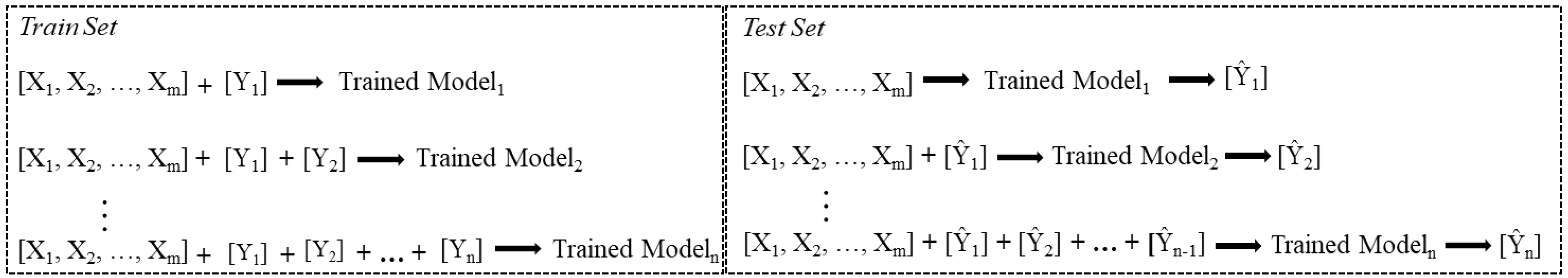
2.4. Data Reconstruction Method

On inspecting the in situ vertical time series profiles of water temperature (WTMP), salinity (SAL), and current velocities (CS), WTMP and SAL had 5% missingness, while large contiguous segments of data were found missing in CS, which roughly comprised 20% of the entire series (Figure 3). Although studies have shown that some statistical methods can credibly impute datasets having up to 30% missingness [35], such methods do not consider the temporal correlations (lagged dependencies), or seasonal patterns required to model a time series. In such cases, autoregressive time series models could be used for the reconstruction. Nevertheless, those parametric models depend on the estimation of the lag, difference, and the size of the moving average window parameters that are not updated (or skipped) for the missing portions [36,37], and, hence, are not suitable for complex multivariate data. Therefore, hybrid models or data-driven algorithms are used as tools to reconstruct and analyze incomplete time series [38]. Here, we have compared the time series reconstruction efficacies of two boosted tree-based models, the Gradient Boosting Regressor (GBR) and the Extreme Gradient Boosting (XGBoost) algorithms.

2.4.1. Model Description

The GBR is a machine learning algorithm that performs supervised classification and regression tasks. It is a tree-based model; however, unlike the Random Forest (RF) algorithm, which is built on completely random subsets of data and features, the GBR trains multiple models in a gradual, additive, and sequential manner by putting more weight on instances with wrong predictions and high errors. Thus, the learning is focused on improving the predictability for the instances that are hard to predict, and by stochastically training each tree ensemble on a different subset of the training sample, the model generalizability tends to improve. Since the GBR works on the gradient descent optimization procedure, the hyperparameters include learning rate (the step size for descending the gradient), shrinkage (reduction of the learning rate), and loss function (MSE), in addition to the hypermeters used for RF modeling, like the number of trees per ensemble, the number of observations in each leaf, tree complexity and depth, etc. Despite being largely implemented for very high predictive accuracy [39,40], the GBR at times suffers from over-fitting; hence, its more regularized variant, the XGBoost algorithm, is sometimes preferred due to its better performance and generalizability [41]. In XGB, the regularization term controls the complexity of the model, which helps us to avoid overfitting [42].

2.4.2. Model Training and Evaluation

Since the air–sea interaction at the surface drives the near-surface (and subsurface) gradients in WTMP, SAL, and CS, the reconstruction procedure also required predicting the outcome variable for a given depth level as a function of its patterns in the layers above it. Therefore, using the GBR and XGBoost as the baseline regressors, two separate regressor-chain models were executed (and compared) for reconstructing each variable’s vertical profiles. A regressor chain is an extension of a multi-output regression model, where a sequence of dependent models is developed to match the number of outcome variables to be predicted (Figure 4). The prediction from the first model is taken as part of the input to the second model, and the process of output-to-input dependency repeats along the chain of models [43].
There were 19 distinct outcome variables (corresponding to the 19 depth levels) for each predicted feature, while the same set of surface variables was used as the input for each of the 6 regressor chains. In the current speed time series, all the observations between 10 March–20 April 2020 were found missing across all the depth levels from 3 m to 20 m. Therefore, the remaining portion of the multivariate time series was used for predictive analyses. Before model training, the input and the output feature sets were separately normalized between 0 and 1, and through 5-fold (without shuffling) cross-validation, the hyperparameters of the regressor chains were fine-tuned. The same procedure was followed for modeling the regressor chains for WTMP and SAL attributes as well, and for each attribute, the last 7 days of data were used for testing the model performance. Across all the models, the loss function was Mean Squared Error (MSE), the number of trees—500, maximum depth—10, learning rate—0.1, shrinkage—0.3, and the remaining hyperparameters were set to their defaults in the ensemble learning and XGBoost Python (version, 3.9.10) modules. Thus, the chained regressions resulted in 19 complete time series for CS, WTMP, and SAL features, and the test predictions were evaluated using the metrics, Mean Absolute Percentage Error (MAPE, Equation (1)), and Root Mean Squared Error (RMSE, Equation (2)).
M A P E = 1 N i = 1 N y i y i ^ × 100
R M S E = M S E
where y i ^ is the predicted value of the target, y i is the ith observation in the sample space of size, N.

2.5. Multi-Output Multi-Step Forecast

In this step, the reconstructed profiles of WTMP and SAL were utilized for multi-step-ahead forecasting of the current speeds for each depth level, using two different deep learning architectures. Due to the higher accuracy and adaptability gained in incrementally learning complex non-linearities (i.e., the hierarchical feature representations) in large multivariate datasets, hybrid deep learning frameworks are leveraged for simultaneously predicting multiple outputs from parallel multivariate inputs. Here, two variants of the CNN-LSTM hybrid network, typically used for sequential learning [44,45], are compared for 1-day-ahead forecasting of CS for all the 19 vertical layers, from an input feature set comprising the corresponding WTMP and SAL values. The two hybrid deep learning architectures are a CNN-LSTM encoder–decoder network and a multi-head CNN-LSTM network.

2.5.1. CNN Architecture

A convolutional neural network (CNN), or ConvNet, specializes in highly abstracted features of objects from visual data, or any data that can be represented with a gridded topology. A typical CNN architecture has three layers: a convolutional layer, a pooling layer, and a fully connected (FC) layer. The convolution layer is the building block of a CNN, since it helps extract various features from the input data by performing a dot product between the kernel and the window of data, in a sliding manner, to obtain the convolved output, which is fed to the pooling layer. The pooling layer reduces the feature map dimension and extracts dominant features by summarizing the data for each slice of operation, as per the pooling functions defined by the user in every pooling layer. By flattening the pooling layer outputs into a single dimension, the learned features are passed to the FC layer to get the predicted outputs. Different CNN architectures are built with varying combinations and stacking of these layers and are based on the number of dimensions along which the kernel slides; a CNN model could either be 1-dimensional (Conv1D), 2-dimensional (Conv2D), or 3-dimensional (Conv3D). While the Conv2D- and Conv3D-based architectures are prevalent in computer vision [46], the Conv1D models are used for sequence learning like time series forecasting, which requires the kernel to slide only along the 1-dimension, the time axis [47].

2.5.2. LSTM Architecture

The long short-term memory (LSTM) model is a preferred variant of the recurrent neural network (RNN) architecture mostly used for time series forecasting. It processes sequence data by looping over time steps and learning the long-term dependencies better than an RNN, while also overcoming the vanishing and exploding gradient problems [48]. The building blocks of an LSTM network are the memory blocks called cells, and three gated operations (forget, input, and output) are used to define the current and hidden cell states at each time step. On vertically stacking the LSTM cell sequences, information flow across the depth of the network is triggered via the intermediate activation functions connections, until the dense layer assimilates all of that to make the final prediction. A typical LSTM cell structure and computation of the cell states for multi-step wave height forecasting from buoy data is illustrated in [49].

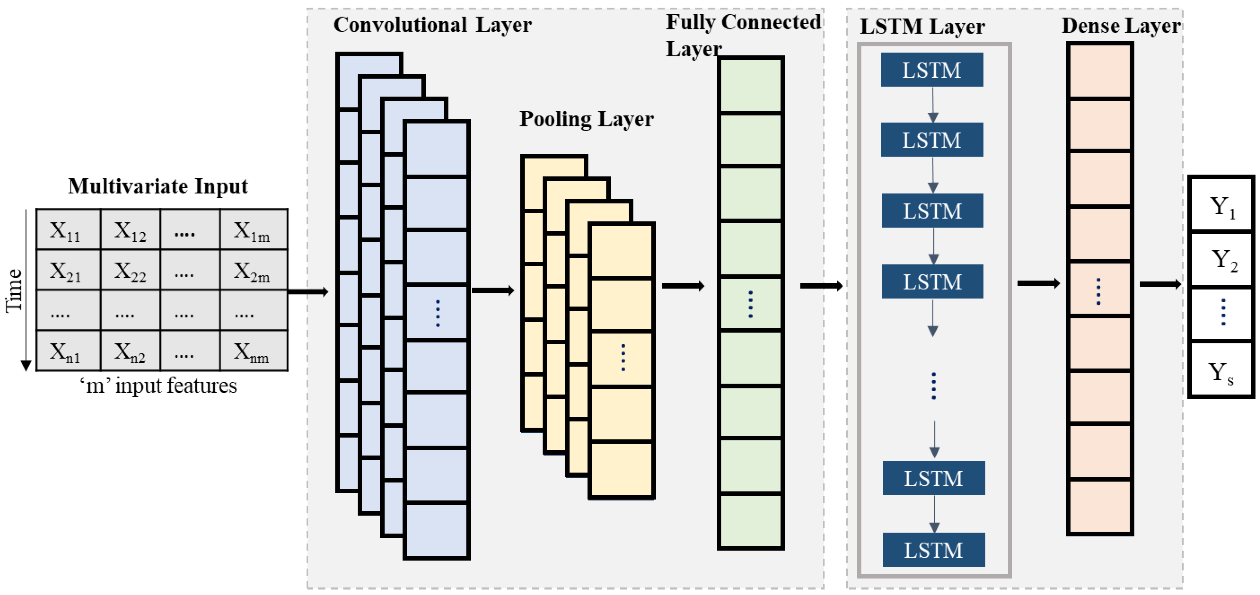
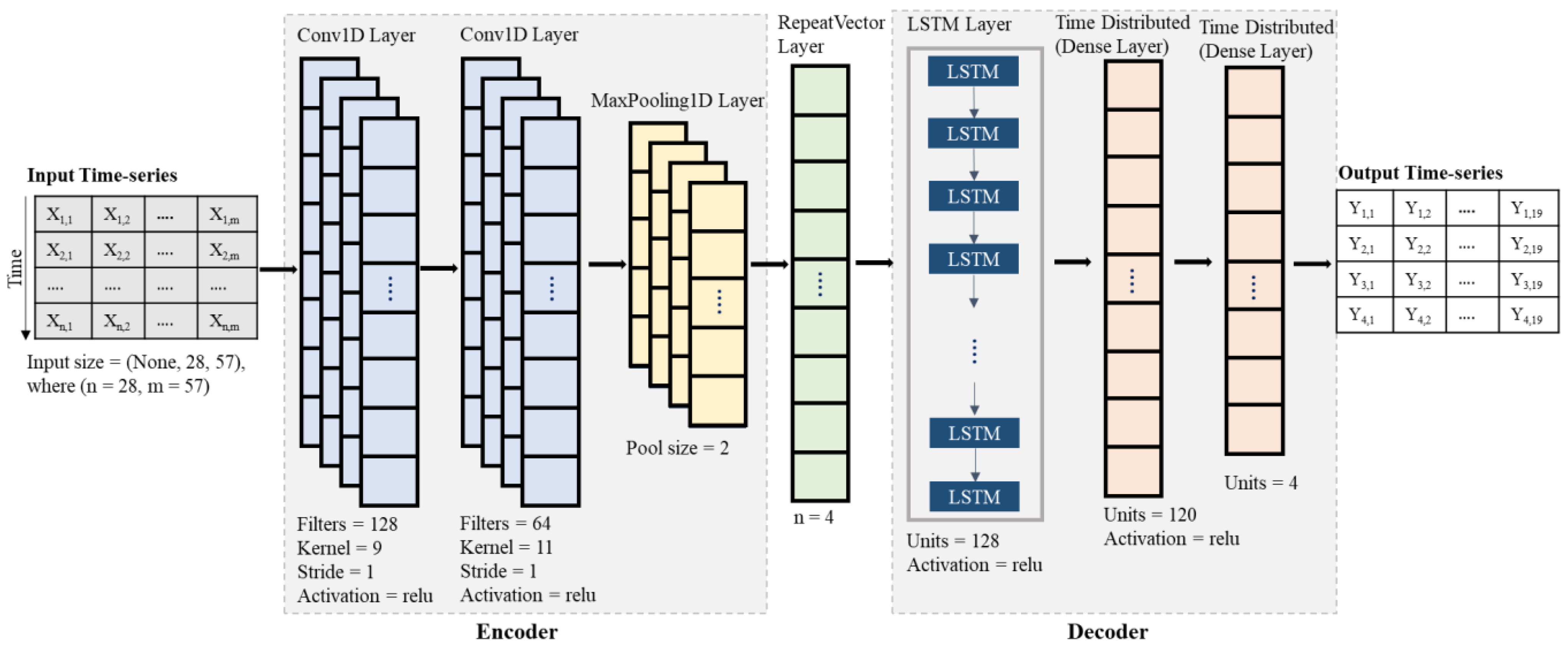
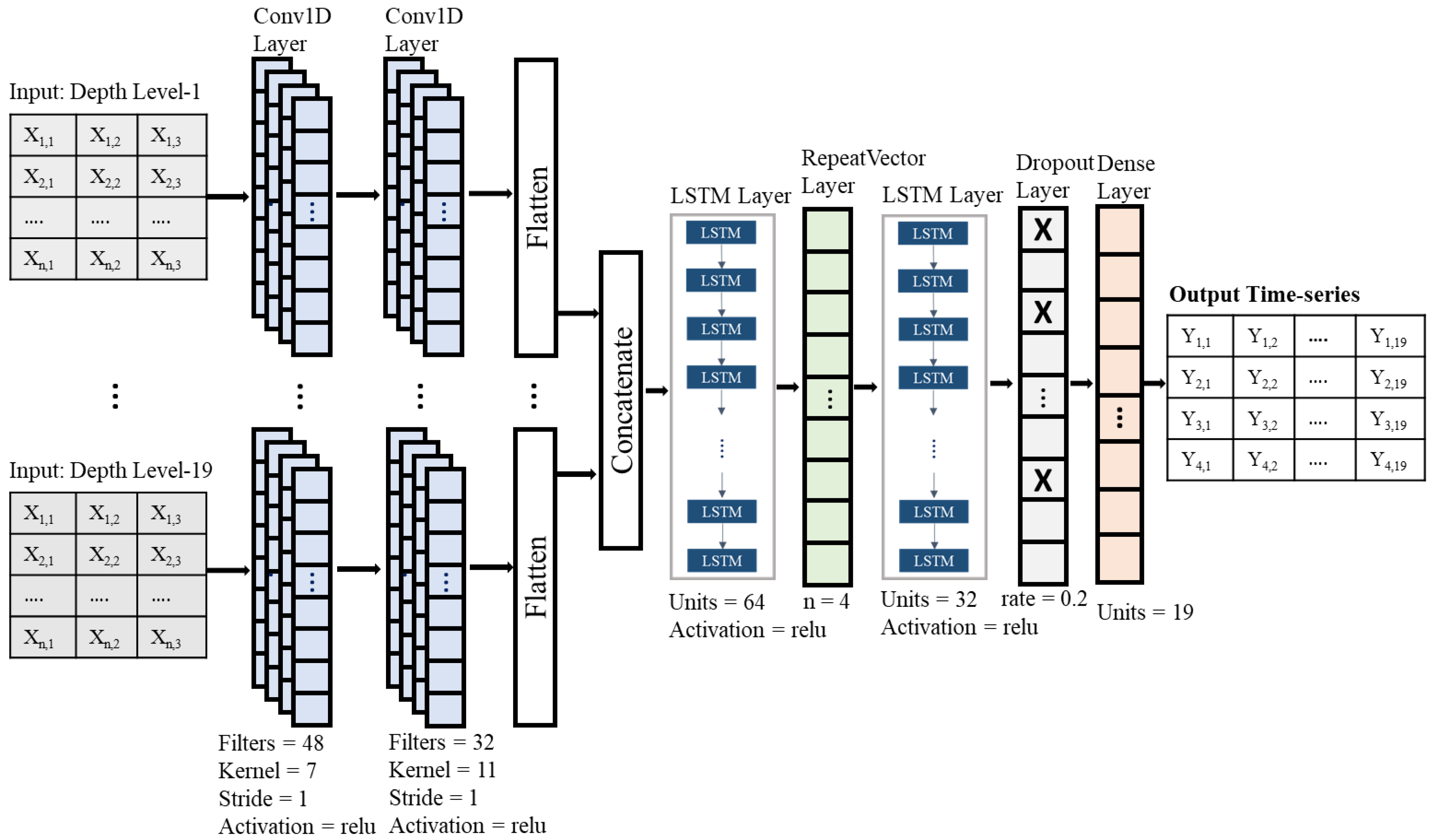
2.5.3. CNN-LSTM Architecture

In a hybrid CNN-LSTM model (Figure 5), the outputs of the CNN layers are passed to the LSTM layers, followed by a dense layer at the output to support sequence prediction. Thus, the LSTM layers can be supported with informative high-level features learned by the CNN layers, instead of directly learning the temporal patterns from raw data. In this work, the hybrid CNN-LSTM models were built using the TimeDistributed and RepeatVector layers of the Keras deep learning Python (3.9.10) API [50]. The TimeDistributed layer is a wrapper that allows us to apply a layer to every temporal slice of an input while building models with one-to-many or many-to-many architectures. Further, a RepeatVector layer is used to repeat the inputs n times, where n is the number of time steps to be predicted for each output, or simply the forecast range.

2.5.4. Forecast Model Architecture and Configuration

CNN-LSTM encoder–decoder network (Model-1): In this model, the ConvNet layers acted as the encoder, and the LSTM layers as the decoder of the encoder–decoder network. An encoder–decoder architecture is typically used for variable-length sequence-to-sequence (seq2seq) learning [51,52]. The encoder takes a variable-length sequence as input and transforms it into latent representations, summarized as a fixed-length vector. The decoder then interprets and maps the encoded state to a variable-length output sequence. Thus, in this case, the encoder was fed with a 3-dimensional input (CS, WTMP, SAL) from each depth level to forecast the 1-day-ahead CS values. And given the 6 h sampling interval of the input data, this implied 4 time steps forecasted for each of the 19 CS time series. As shown in Figure 6, the encoder component of the model consisted of two subsequent Conv1D layers with 128, 64 filters, and kernels of sizes 9, 11, respectively. The second Conv1D layer was followed by a max pooling layer, the output of which was flattened and provided as the input to a RepeatVector layer. This ensured that the output context vector was repeated four times (n = 4, the range for 1-day-ahead forecast) and provided as input to the decoder part, an LSTM layer with 128 units. Finally, the TimeDistributed wrapper applied on an FC dense layer was added to separate the LSTM layer’s output for each of the 4 time steps in the forecast range, resulting in an output dimension, 4 × 19. The Rectified Linear Unit (relu) activation function was used to activate the neurons in all the network layers.
Multi-head CNN-LSTM network (Model-2): This model (Figure 7) exploits multiple Conv1D layers to extract a separate set of convolved features for each variable in the multivariate time series input. Each separate CNN is an independent ‘head’, which are successively flattened, concatenated, and then reshaped to match the input shape of the LSTM layer [53]. Since this architecture leverages multiple CNN heads, unlike a common multi-channel structure, it is hypothesized to offer better forecast accuracy and explainability by more successfully extracting the informative features specific to each input series. The CNN head for each time series had two Conv1D layers with 48, 32 filters, and kernels of sizes 7, 11, respectively. The CNN configuration was the same for all the 19 depth levels, so that the same number of features are obtained for every input to the CNN. The flattened outputs of the CNN heads were concatenated and passed as input to a 2-layer-deep LSTM stack with 64 and 32 units, respectively. The two LSTM layers were connected by a RepeatVector layer with n = 4, for the 4 steps ahead. Finally, with a 20% drop out of the second LSTM layer outputs, the final forecasted values were obtained after being passed through a dense layer with 19 output neurons. Like Model-1, relu activation was used for all the ConvNet and the LSTM layers.

2.5.5. Data Preparation

The CS, WTMP, and SAL time series from each depth level were structured as a multi-index pivot table (Figure 8) representing the multivariate parallel time series input to the multi-output forecast models. This hierarchical data representation ensured that the interrelationships between a variety of input features (or predictors) from different depth levels were accounted for while forecasting the vertical profiles of CS. For model training, we used approximately 9 months’ worth of data from the available period from September 2019 until June 2020, and the remaining time series comprised the test set. Before feeding the data to the models, the train and test feature sets were normalized and transformed using a scale of [0, 1] to overcome the potential bias in the predictions caused by the differences in the scales of input features. Further, to enable temporal feature learning, 28 lagged variables (i.e., data from the past 7 days) were included for each input feature, such that for each time step the input matrix dimensions were 28 × 57 (3 variables from 19 depth levels).

2.5.6. Model Training and Evaluation

Model training was performed on the transformed train set, out of which the last 10% data series was used for validation. The input feature maps of both the models were obtained from the sliding convolutional operations that were max-pooled and provided as flattened inputs to the LSTM layers. With a batch size of 16, both the models were trained for 500 epochs, which implied that during each epoch, the model parameters were updated after every 16 training samples were processed. During backpropagation, the model weights were optimized by minimizing the MSE loss function at a learning rate of 0.001 using the stochastic Adam optimizer [54]. Both the models utilized the walk forward validation approach, which is known to prevent overfitting and widely used for multi-step forecasting [55,56]. To regularize the training process, the performances of both the networks on the validation set were monitored, and further training was stopped if the validation loss failed to lower after 10 consecutive epochs. After the models were trained, forecasts were obtained for the test set, and the forecasted values inverse transformed to the original scale. Comparative analysis of the forecast ability of the hybrid models was then performed based on three performance metrics, RMSE, MAPE, and the coefficient of determination (R2, Equation (3)). Finally, the statistical and the time series features were derived for the raw test data and the forecasted time series for comparative assessment. The time series features, described in Hyndman et al. [57], were calculated on tiled (non-overlapping) windows of size 4 (i.e., on 1 day’s data).
R 2 = 1 y i y i ^ 2 y i y ¯ 2
where y i ^ is the predicted value of the target, y i is the ith observation in the sample space of size, N, and y ¯ is the mean of y.

3. Results and Discussion

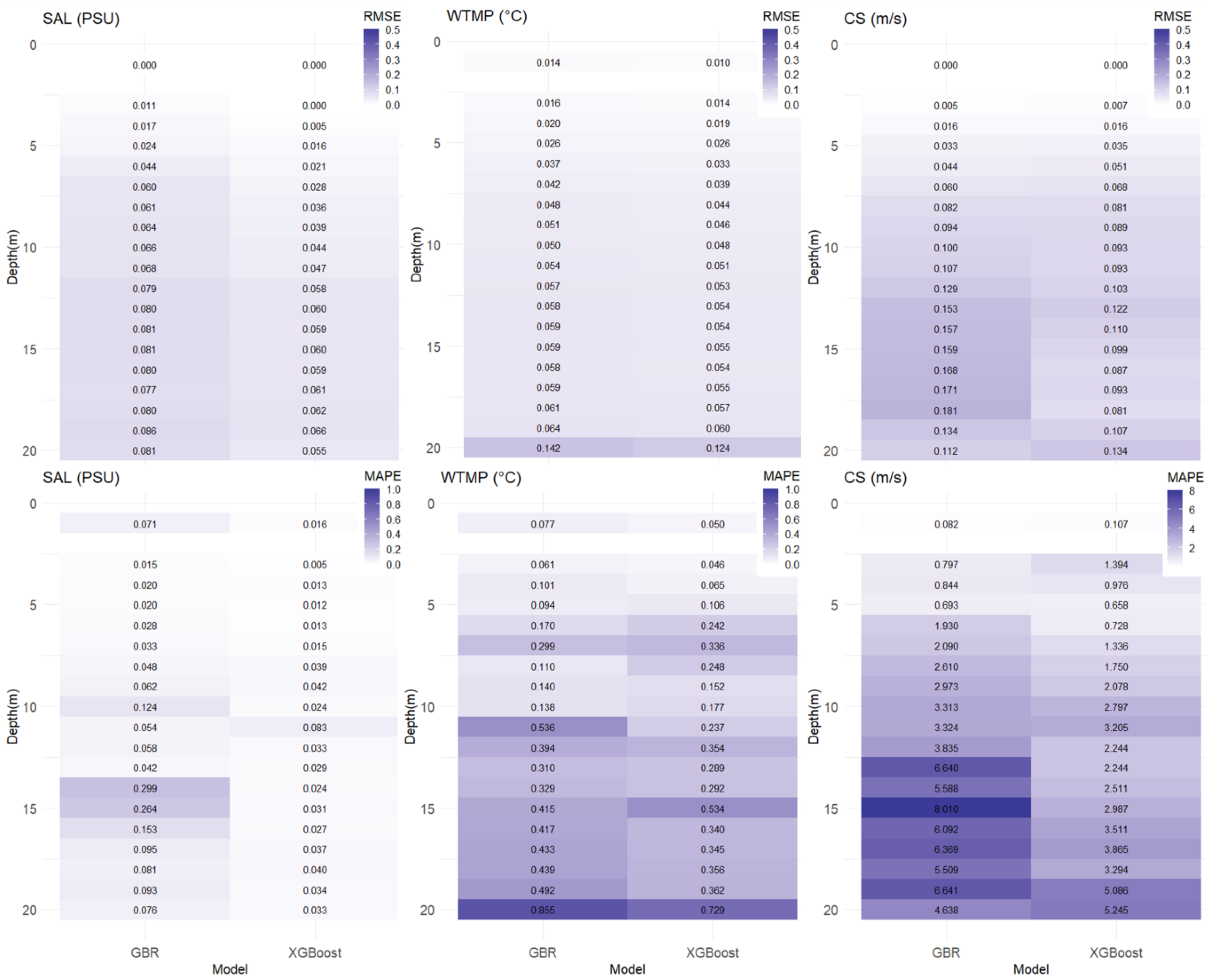
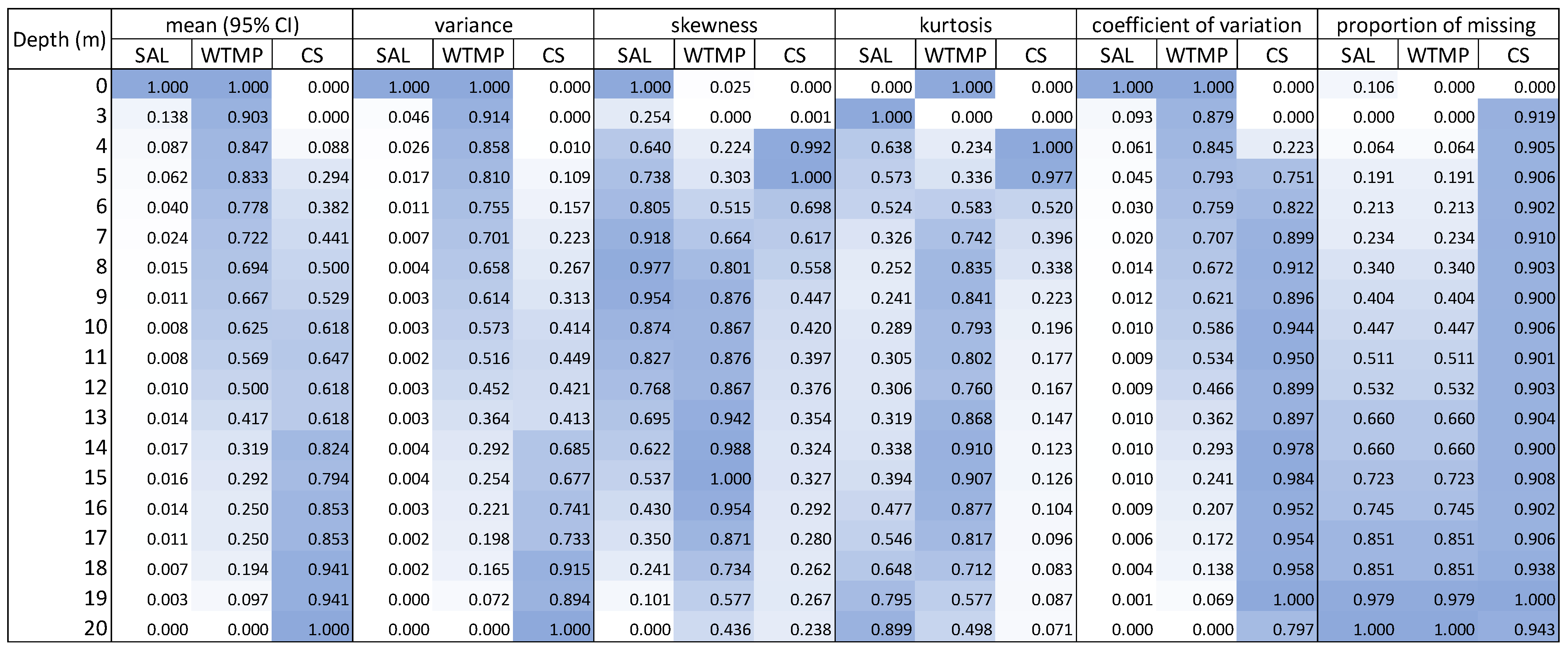
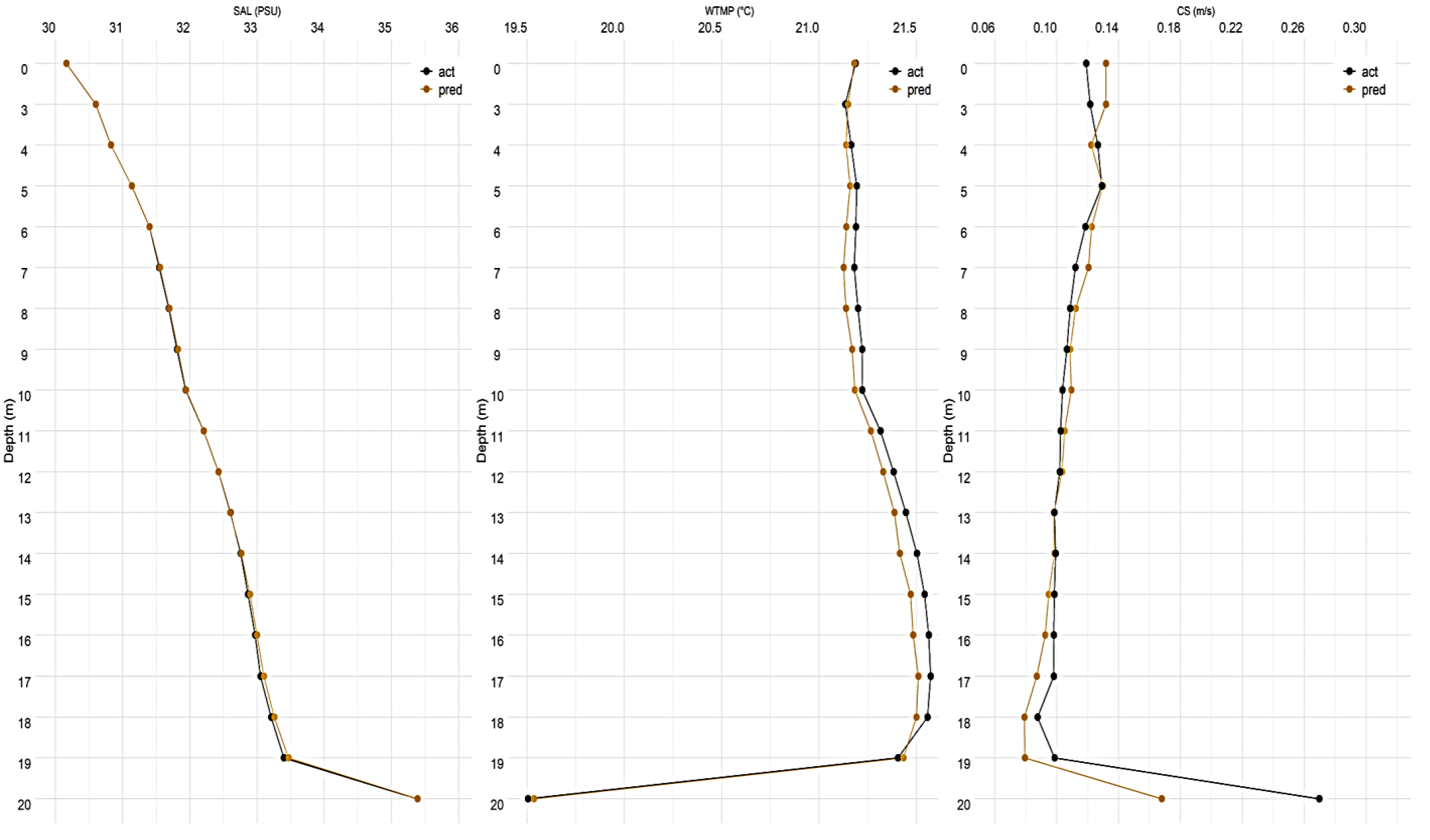
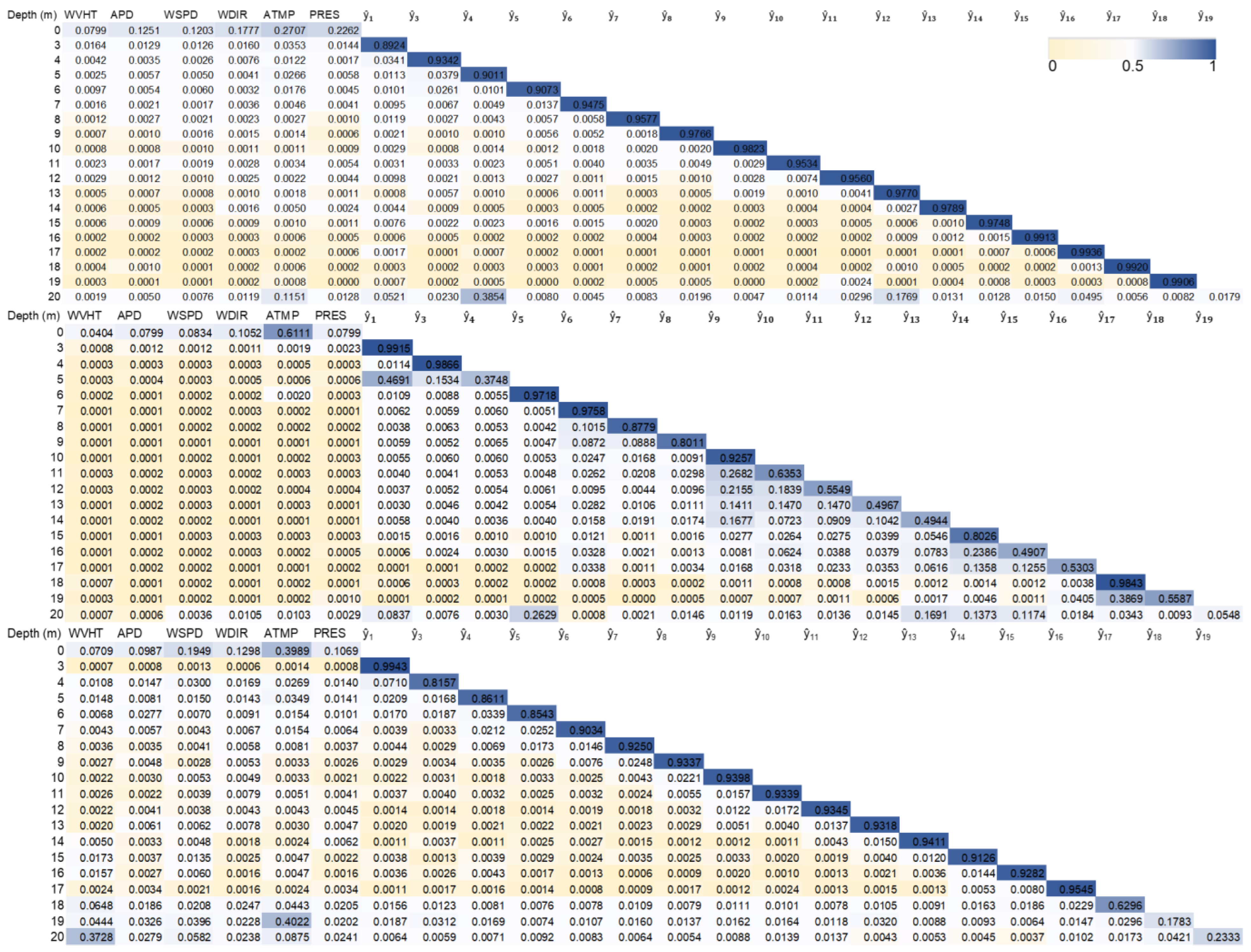
3.1. Reconstruction Performance

Comparison of the GBR and XGB model performance in reconstructing the three variables revealed that both the models had minimal differences in the case of SAL and WTMP, whereas XGB performed remarkably better than the GBR in CS data reconstruction. In addition to being faster than gradient boosting, due to its ability to robustly deal with sparse learning data, XGB has reportedly been most effective in prior data reconstruction studies [41,58]. Also, per overall comparison, the XGBoost model yielded lower errors, with a maximum RMSE of 0.066 PSU, 0.124 °C, and 0.134 m/s, and highest MAPE estimates of 0.083%, 0.729%, and 5.245% for SAL, WTMP, and CS, respectively (Figure 9). These results showed that the CS reconstruction performance was remarkably lower than that of WTMP and SAL. Such results were expected given the higher proportion of gaps in the raw CS time series. We also noticed that SAL reconstruction performance was better than that of WTMP, although both had the same proportion of missing data. This difference could be attributed to the higher variability inherent in the raw WTMP data, as identified from the comparative analysis of the summary statistics (variance and coefficient of variation) of the raw profile data (Figure 10). Further, relatively higher skewness and kurtosis in WTMP also implied that the observed data points had more extreme values and a heavy tailed distribution, compared to that of SAL. And, although the XGB performance seemed largely consistent across the depth layers, slightly higher errors were noticed for the deeper layers, especially in case of CS.
Visual assessment of the mean actual and reconstructed time series further demonstrated that the vertical profile patterns could be correctly modeled by the XGB algorithm for the three variables (Figure 11). The salinities of the coastal waters were in the range from 30.1 to 35.4 PSU, and linearly increasing by a mean 0.5 PSU with every layer deeper down to 19 m below the surface. At 20 m deep, a sharp 2 PSU increase in salinity was observed, which was also correctly modelled by the XGB algorithm. At 19 m deep, such breakpoints in the vertical profiles of WTMP and CS were also observed. Nevertheless, unlike SAL, down to 19 m from the surface, WTMP and CS profiles had low anomalies and almost uniform variation, ranging from 21.2–21.6 °C, and 0.9–0.13 m/s, respectively. Beyond that depth level, WTMP plunged by 1.7 °C, while CS rose from 0.12–0.27 m/s. Similar patterns in the vertical profiles of SAL and WTMP can be found in Lobus et al. [59]. Such drastic changes in the vertical profiles possibly imply the presence of a pycnocline at around 18–19 m deep, resulting in the mixing up of SAL and WTMP along the gradient indicated by the spike in CS at that depth. Additionally, since the mooring depth was 20 m, these changes in the bottom layer could represent a salinity barrier later due to transport from the deeper offshore area [60]. Hence, we could infer that the abrupt distributional shift in CS data along with large contiguous data gaps could have resulted in the underestimation of CS for the last two depth levels (Figure 11). The complete reconstructed CS time series at various depth levels are illustrated with the actual data, clearly identifying the underestimated portions in the time series (Figure 12). In Figure 13, the importance of each input feature and for each depth level is represented using the gain scores. In tree-based models, gain implies the relative contribution of the corresponding feature to the model calculated by taking each feature’s contribution for each tree in the model. A higher value of this metric when compared to another feature implies it is more important for generating a prediction [42]. The feature-importance scores demonstrated the importance of utilizing a chained regression approach for vertical profile data reconstruction, since, beyond the surface layer, for every variable, the previously predicted outcome was found to be highly significant for the next prediction. As expected, diminishing feature importance of the surface characteristics was noticed beyond 9 m deep, especially in SAL and CS. It was interesting to note that at the depth levels 18, 19, and 20 m, the relative importance of the surface characteristics abruptly increased, whereas that of the previous layer’s CS predictions dropped. These results further corroborated our earlier inference of the possible presence of a pycnocline and mixing along the water column at that depth.

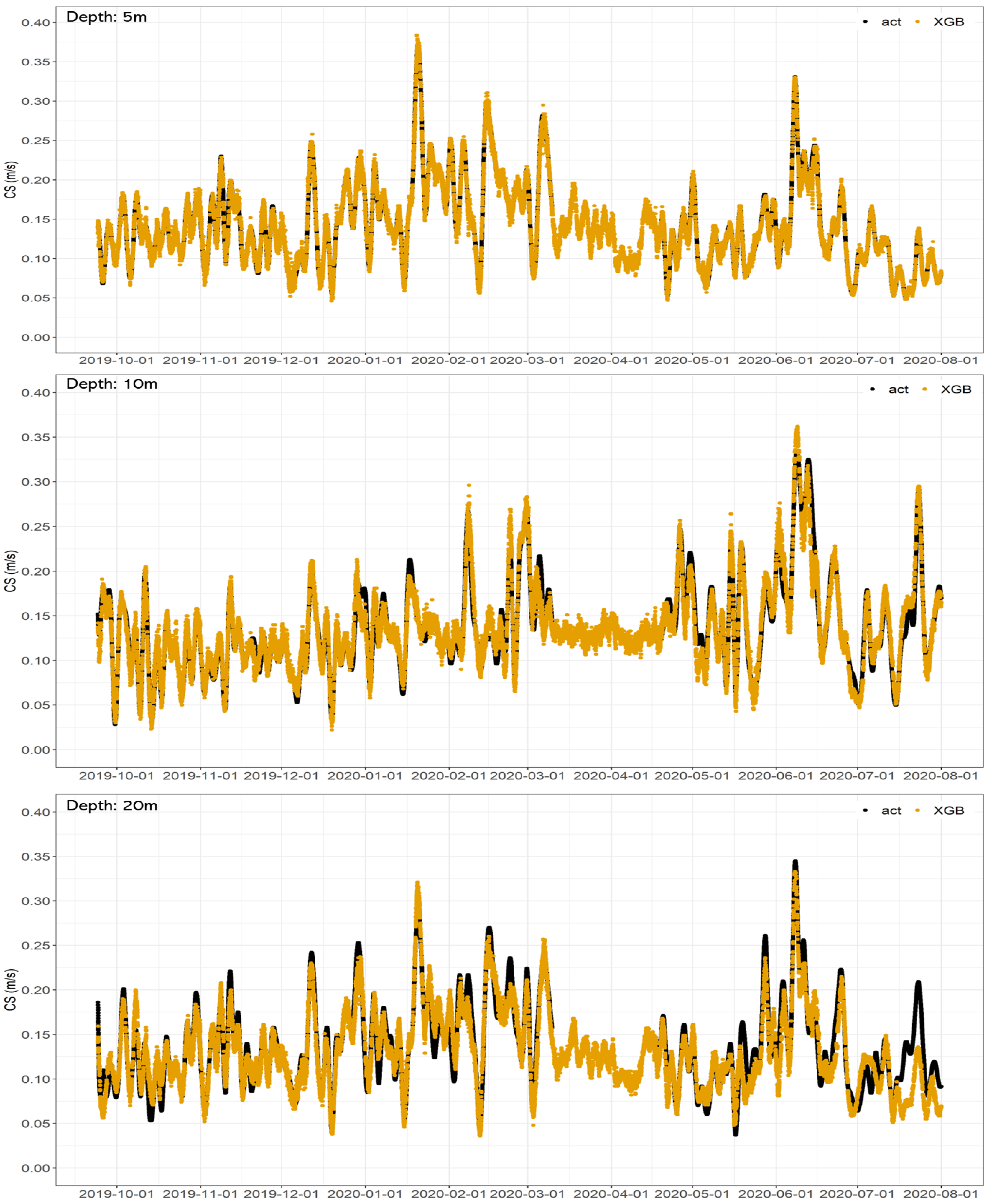
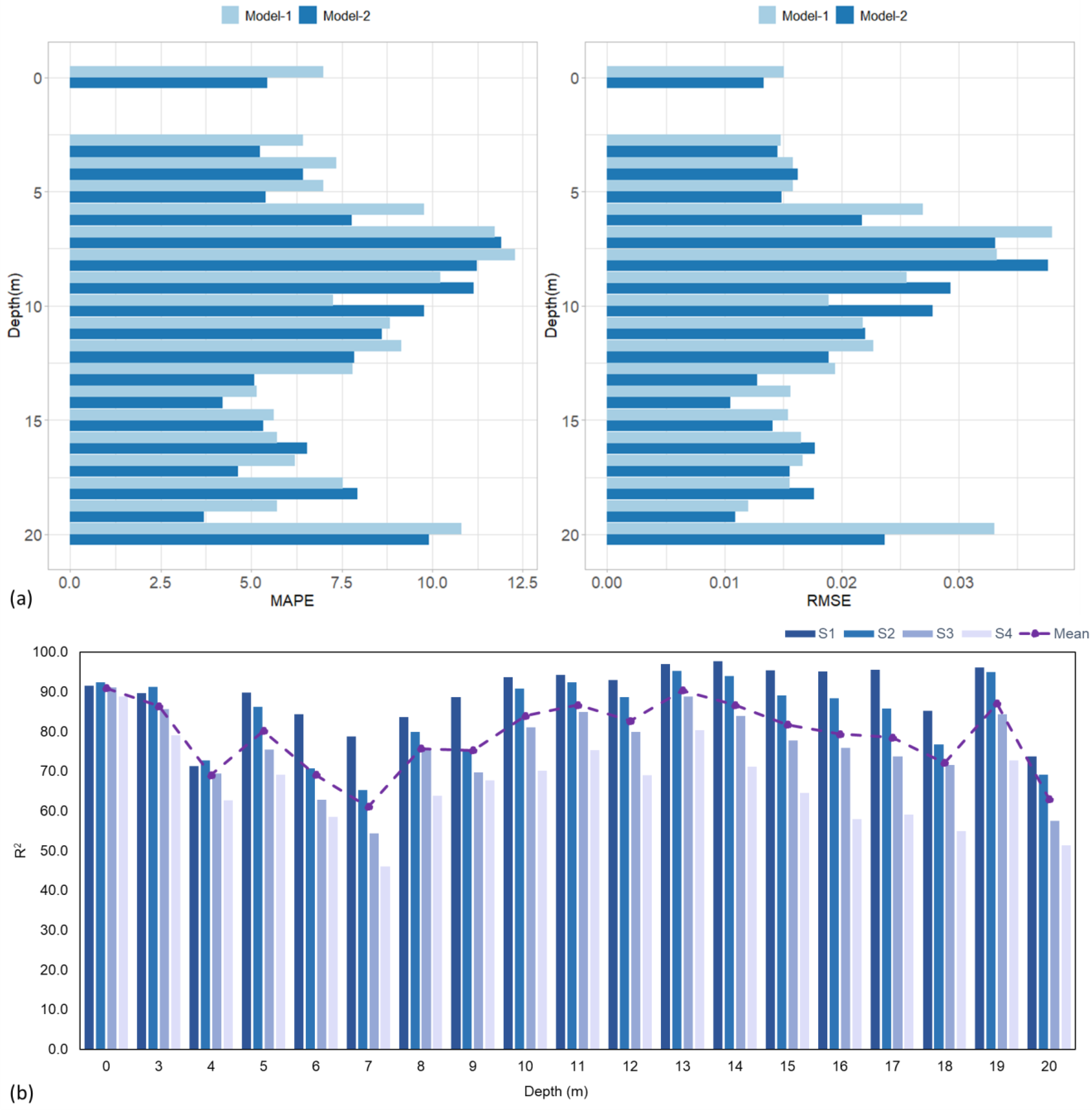
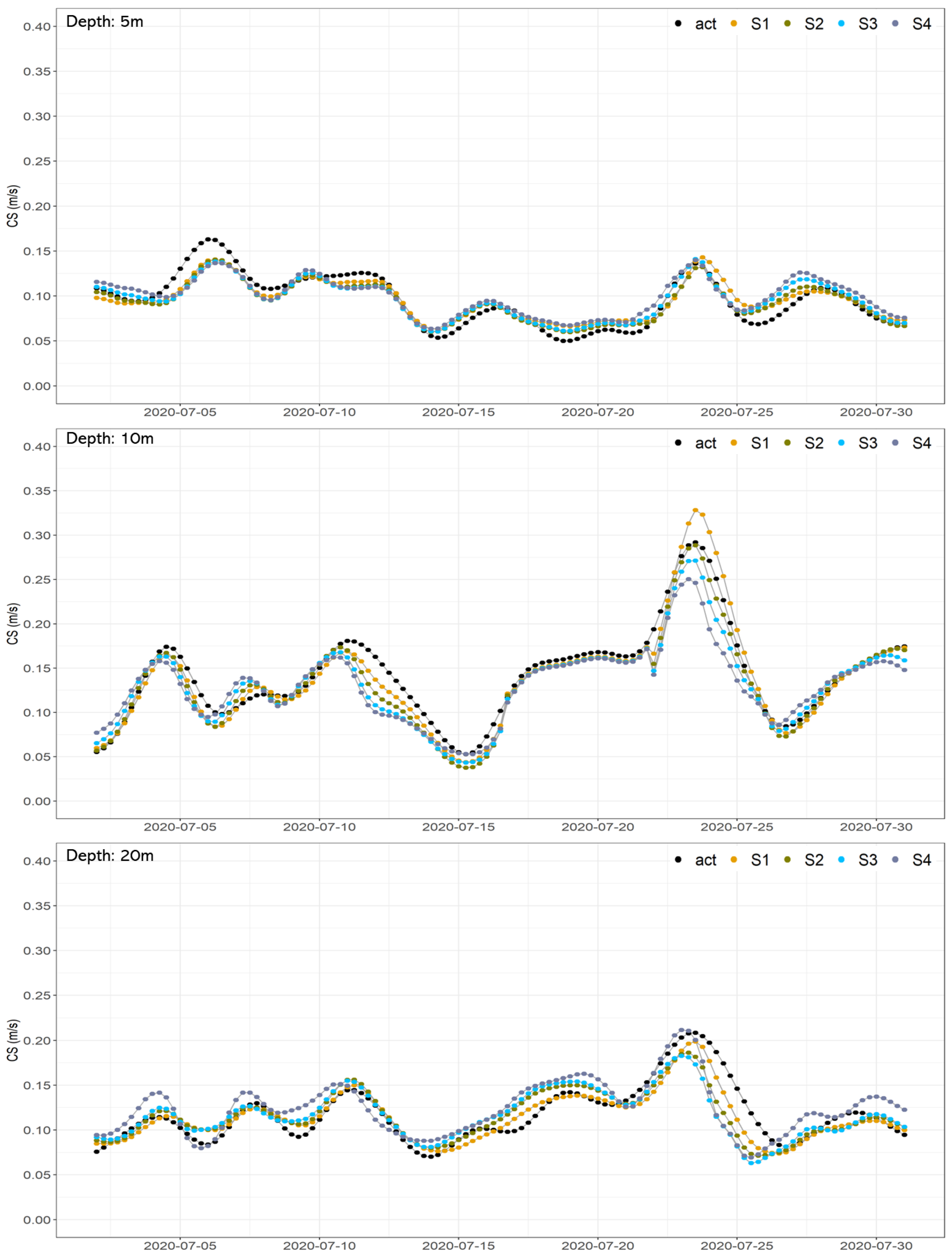
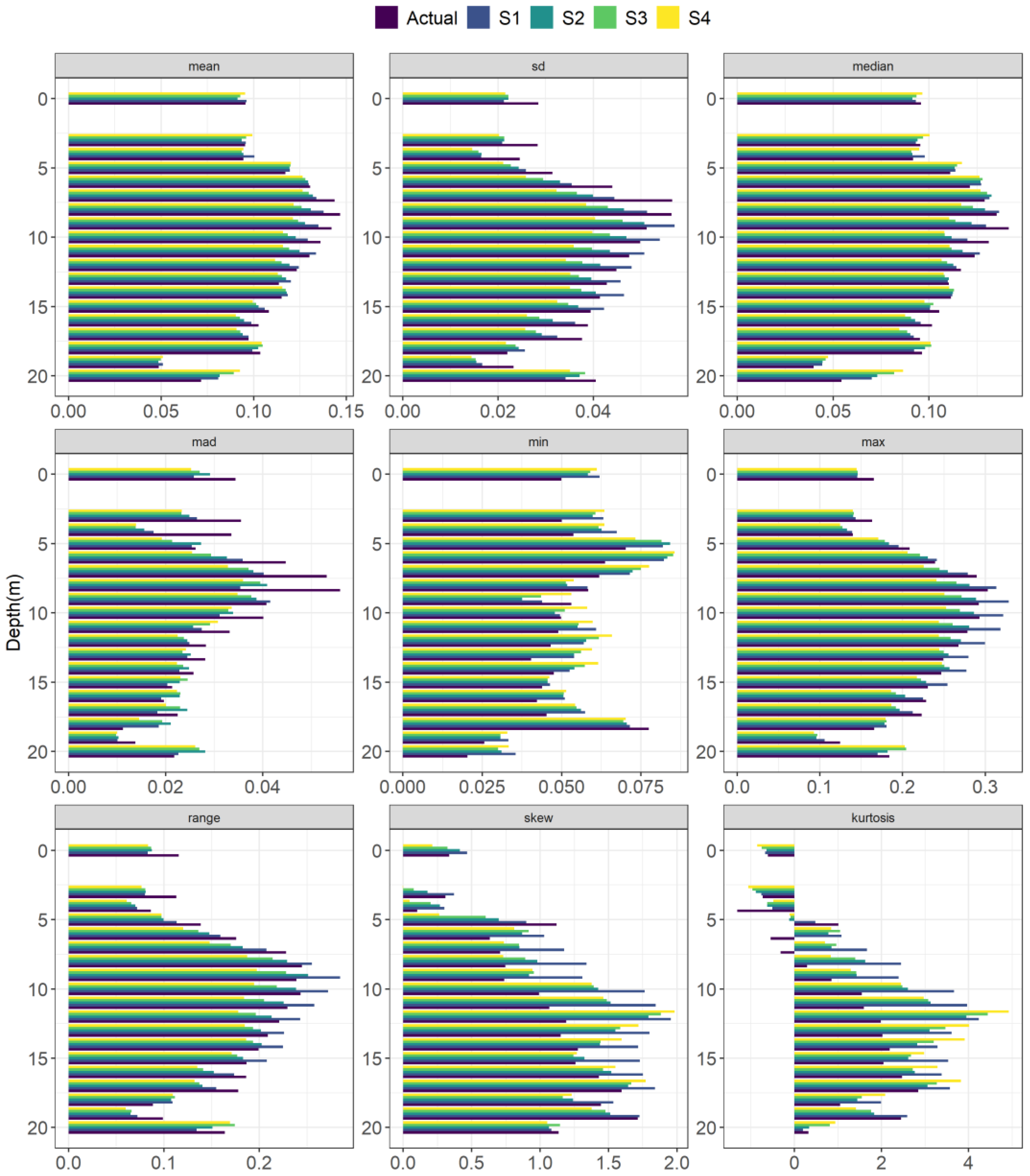
3.2. Multi-Step Forecast Performance

Our results on the multi-step forecast of CS demonstrated an overall better performance achieved by the multi-head CNN-LSTM network (Model-2), although for some depth layers Model-1 scored better (Figure 14a). On average, Model-2 was able to achieve 0.7% less MAPE, and the RMSE was lower by 0.001; hence, it was chosen for further analysis. The minimum MAPE scores for Model-1 and Model-2 were 5.15% and 3.7%, while the maximum MAPE scores were 12.28% and 11.96%, respectively. Regarding the mean goodness of fit scores (Figure 14b), Model-2 could explain approximately 80% of the proportion of variation in the test data across all the depth levels. The forecasted time series for each step size are compared with the test data from different depth levels in Figure 15, illustrating the gradual increase in error (or underestimation) as the step size increased, which is usually noticed with multi-step sequential networks [60].
The forecast model’s performance was found to be consistent with our previous inferences (observed in the reconstruction results). From the resultant R2 estimates, we could again associate the change points along the water column with that of the mean CS profiles (refer Figure 11). As the water depth increased, the forecast error seemed to suddenly spike at 6 m and 18 m, implying abrupt changes in the physical properties along the water column at those depth levels. Therefore, although an overall data summary is illustrated in Figure 9, to further examine the validity of our findings from the forecast analysis, we have compared the statistical and the time series features of the actual test data and each of the multi-step-ahead forecasts (Figure 16 and Figure 17). We noticed a striking similarity in the vertical patterns of the test data statistics, and the forecasted metrics.
The descriptive features were the mean, standard deviation (sd), median, median absolute deviation (mad), minimum (min), maximum (max), range, skewness (skew), and kurtosis. The time series features were trend, stability, linearity, curvature, entropy, the largest shift in Kulback–Leibler divergence between two consecutive windows (max_kl_shift), the time index of the max_kl_shift (time_kl_shift), and the first autocorrelation coefficient of the time series (x_acf1). The descriptive statistics (Figure 16) revealed that in the test data, not only the overall magnitude, but also the variance in the current speed significantly increased from 6 m deep downwards until 10 m, subsequently following a declining trend down to 18 m deep. Therefore, the mean, maximum (max), median, standard deviation (sd), median absolute deviation (mad), and range followed similar patterns, that was reversed in case of the minimum observed CS values. Consequently, as the water depth increased beyond 5 m, we found that the test data had a more skewed distribution with higher kurtosis. These differences in the physical properties of CS values could also be confirmed from the profiles of the time series features (Figure 17)—stability, linearity, curvature, and the maximum Kulback–Leibler shift (max_kl_shift), which denoted the variance or divergence between two consecutive time windows. Finally, vertical profiles of the statistical and time series properties of the forecasted values from each step size (S1, S2, S3, S4, representing 6, 12, 18, 24 h ahead lead times, respectively) were found to exactly follow that of the raw test data (albeit with slight differences among them, as observed in the forecasted metric comparison). Hence, we could infer that while the proposed model optimally learned the data properties at each depth level, increased error for the depth levels denoting break points in the vertical current profile also implied the model’s sensitivity to the distributional shift in the unseen test data.
Per the literature, several deep learning-based studies on forecasting vertical profiles of such physical ocean properties have reported very high model performance scores, and for deeper ocean conditions [25,26]. Such studies generally rely on a considerable amount of historical data for model training, such that the model can learn the inherent trends and seasonalities of the sequential data better, along with the complex high-level features, resulting in better model performance and generalization. For example, in Kar et al. [47], we have presented that with 10 years of training data, we could forecast wave heights from the same Viking buoy data (only surface characteristics), 72 h in advance, with ~97% mean R2. However, here, we had 10 months of training data, and our proposed model (Model-2) could still demonstrate excellent predictive ability, with a 7.2% mean MAPE, and 0.0195 mean RMSE, for 24 h ahead forecasts. Hence, given the limited length of the time series in our case study, we believe the satisfactory forecast performance could be attributed to the model architecture.
To enhance the predictive power of a machine learning model, constrained with limited training data, it is often beneficial to feed the model with informative (additional) features. Therefore, in the absence of sufficient historical features, we leveraged multiple CNN models for each of the multivariate inputs, such that independent convolved features from each time series could aid the LSTM forecast ability. Prior works [61,62] on sequential deep learning from limited training data have leveraged convolutional models for data augmentation and enhancing the input feature set of the LSTM network for various other applications. For example, Widiputra et al. [60] have trained a multi-head CNN-LSTM network on 242 days of past data for financial time series forecasting, and reported 0.017 mean RMSE. Thus, we base these results off of two key modeling perspectives: training data length and model architecture.
Finally, it is crucial to note that the neural networks applied were trained on the data from the northern Gulf of Mexico, which is subjected to the intense freshening by the Mississippi water, resulting in the strong subsurface barrier layer, which makes it different from the southern Gulf and adjacent Atlantic. Hence, when applying them to other basins, learning should be repeated, and models need to be trained as per the water characteristics in those locations. Previously, current speed forecasts have been performed for different regions using both simple and complex neural network prediction models. For example, with a single-hidden-layer feed-forward backpropagation network, for a 12 h ahead forecast, the resultant mean RMSE was 0.15 m/s [63], and deep bi-directional LSTMs have been beneficial in achieving RMSEs of less than 0.021 when compared for multi-step forecasts across multiple locations [64]. Immas et al. [65] have reported that deep LSTM models and transformer models (which are more complex networks) have comparable forecast performances, resulting in an averaged normalized RMSE of 0.10 and 0.11, respectively. And in this case study, we could achieve a 0.0195 mean RMSE with a limited dataset of just 10 months, suggesting excellent predictive ability and the progressiveness of the proposed multi-head CNN-LSTM model. Prior research also corroborates the superior predictive ability of CNN-LSTM-based models on limited datasets [66]. Additionally, other types of neural network architectures could also be examined for similar forecast applications in different regions [67,68].

4. Conclusions

In this work, we demonstrated a case study on dealing with common sensor data artifacts that can potentially impact the efficacy and accuracy of subsequent predictive modeling. By utilizing the Viking buoy data, which contains several sensors to measure both surface and vertical casts of sea state characteristics, we demonstrated a framework to efficiently handle contiguous gaps in time series profile data of multiple sea physical variables from the surface characteristics. We then utilized the reconstructed data to forecast 24 h ahead CS for all the depth levels. For accurate time series data reconstruction, we proposed an XGB-chained regressor model, and a multi-head CNN-LSTM hybrid model for simultaneous multi-step forecasting of the current speed vertical profiles. Despite the highly dynamic nearshore conditions, and limited experimental data, we could reconstruct CS time series and forecast the profiles 24 h ahead with just 5% and 7% mean error values, respectively. In future, we intend to test the generalization ability of the proposed framework with data from a diverse set of buoys deployed in the CUBEnet region for longer time periods.

Supplementary Materials

The following supporting information can be downloaded at: https://www.mdpi.com/article/10.3390/jmse11101964/s1, Figure S1: Available instruments on the Viking buoy are shown in the image (source: http://www.multi-electronique.com/buoy.html), which are integrated and deployed per user requirement. The list of specific instrument measurements includes conductivity and temperature, oceanographic pH, biogeochemical, acoustic doppler current profiler (ACDP), radiometer, fluorometer, water salinity, water temperature and wavemeter (wave height and period), global positioning, weather (temperature, wind, humidity, rain, atmospheric pressure) wind, light, oceanographic pC02, radar reflector, automatic CTD profiler (for observing conductivity and temperature from depth). The buoy comes with its own software, designed to help the researcher interpret information from the buoy. This information is sent to a land station via cellular modem or satellite or a combination of cellular and Internet, at user-defined time intervals. Here, Iridium satellite uplink was leveraged to receive data every 15 min. For easier deployment using a small boat, the buoy uses only one anchor. Details provided here are sourced from http://www.multi-electronique.com/files/Buoy_specification.pdf; Figure S2: Illustration of the anomalies present in raw current speed data (top), identified using the seasonal and trend decomposition using Loess (locally weighted smoothing) anomaly diagnostic method, and comparison with outlier removed time series for each depth level (bottom). The anomalies identified in the raw data represented sensor noise that amplified with increase in water depth, which were removed to obtain current speeds within a realistic range of 0.6m/s; Figure S3: Wave anomaly diagnostics plotted (L) with respect to the normalized values of wind speed, temperature, pressure and relative humidity, and the correlations between each pair of the surface characteristics are illustrated (R); Figure S4: Comparison of Viking meteorological and wave data with respect to the nearest NDBC buoy data from station 42012.

Author Contributions

Conceptualization, S.K. and J.R.M.; methodology, S.K.; software, S.K.; validation, S.K., R.C. and J.R.M.; formal analysis, S.K.; resources, J.R.M., V.S., S.S. and L.B.; data curation, S.K. and V.S.; writing—original draft preparation, S.K. and G.A.; writing—review and editing, S.K., R.C. and J.R.M.; visualization, S.K.; supervision, J.R.M.; project administration, J.R.M.; funding acquisition, J.R.M. All authors have read and agreed to the published version of the manuscript.

Funding

Funding for this study was supported by The Roger F. Wicker Center for Ocean Enterprise (OE-001), The University of Southern Mississippi, USA.

Institutional Review Board Statement

Not applicable.

Informed Consent Statement

Not applicable.

Data Availability Statement

This data was collected by the Roger F. Wicker Center for Ocean Enterprise research team, and can be found here: http://oceancube.usm.edu/data.html, accessed on 11 June 2023.

Conflicts of Interest

The authors declare no conflict of interest.

References

  1. Kim, J.; Kwon, M.; Kim, S.D.; Kug, J.S.; Ryu, J.G.; Kim, J. Spatiotemporal neural network with attention mechanism for El Niño forecasts. Sci. Rep. 2022, 12, 7204. [Google Scholar] [CrossRef]
  2. Wang, S.; Mu, L.; Liu, D. A hybrid approach for El Niño prediction based on Empirical Mode Decomposition and convolutional LSTM Encoder-Decoder. Comput. Geosci. 2021, 149, 104695. [Google Scholar] [CrossRef]
  3. Wenhai, L.; Cusack, C.; Baker, M.; Tao, W.; Mingbao, C.; Paige, K.; Xiaofan, Z.; Levin, L.; Escobar, E.; Amon, D.; et al. Successful blue economy examples with an emphasis on international perspectives. Front. Mar. Sci. 2019, 6, 261. [Google Scholar] [CrossRef]
  4. Wen, J.; Yang, J.; Wei, W.; Lv, Z. Intelligent multi-AUG ocean data collection scheme in maritime wireless communication network. IEEE Trans. Netw. Sci. Eng. 2022, 9, 3067–3079. [Google Scholar] [CrossRef]
  5. Kar, S.; Sunkara, V.; McKenna, J.; Stanic, S.; Bernard, L. Near Real-Time Radio Frequency (RF) Data Analysis Pipeline for Aiding Marine Domain Awareness and Surveillance. In OCEANS 2022, Hampton Roads; IEEE: Piscataway, NJ, USA, 2022; pp. 1–8. [Google Scholar]
  6. Trice, A.; Robbins, C.; Philip, N.; Rumsey, M. Challenges and Opportunities for Ocean Data to Advance Conservation and Management; Ocean Conservancy: Washington, DC, USA, 2021. [Google Scholar]
  7. Sunkara, V.; McKenna, J.; Kar, S.; Iliev, I.; Bernstein, D.N. The Gulf of Mexico in trouble: Big data solutions to climate change science. Front. Mar. Sci. 2023, 10, 1075822. [Google Scholar] [CrossRef]
  8. Franz, M.; Lieberum, C.; Bock, G.; Karez, R. Environmental parameters of shallow water habitats in the SW Baltic Sea. Earth Syst. Sci. Data 2019, 11, 947–957. [Google Scholar] [CrossRef]
  9. Salles, R.; Mattos, P.; Iorgulescu, A.M.; Bezerra, E.; Lima, L.; Ogasawara, E. Evaluating temporal aggregation for predicting the sea surface temperature of the Atlantic Ocean. Ecol. Inform. 2016, 36, 94–105. [Google Scholar] [CrossRef]
  10. Jonathan, P.; Ewans, K.; Flynn, J. Joint modelling of vertical profiles of large ocean currents. Ocean. Eng. 2012, 42, 195–204. [Google Scholar] [CrossRef]
  11. Srinivasan, A.; Sharma, N.; Gustafson, D. A multi-resolution probabilistic ocean current forecasting system for offshore energy operations. In Proceedings of the InOffshore Technology Conference, Houston, TX, USA, 30 April 2018; p. D031S042R003. [Google Scholar]
  12. Zhu, C.; Liu, W.; Li, X.; Xu, Y.; El-Serehy, H.A.; Al-Farraj, S.A.; Ma, H.; Stoeck, T.; Yi, Z. High salinity gradients and intermediate spatial scales shaped similar biogeographical and co-occurrence patterns of microeukaryotes in a tropical freshwater-saltwater ecosystem. Environ. Microbiol. 2021, 23, 4778–4796. [Google Scholar] [CrossRef]
  13. Bagatinsky, V.A.; Diansky, N.A. Contributions of Climate Changes in Temperature and Salinity to the Formation of North Atlantic Thermohaline Circulation Trends in 1951–2017. Mosc. Univ. Phys. Bull. 2022, 77, 564–580. [Google Scholar] [CrossRef]
  14. Rudels, B. The thermohaline circulation of the Arctic Ocean and the Greenland Sea. In Arctic and Environmental Change; Routledge: London, UK, 2019; pp. 87–99. [Google Scholar]
  15. Kniebusch, M.; Meier, H.M.; Radtke, H. Changing salinity gradients in the Baltic Sea as a consequence of altered freshwater budgets. Geophys. Res. Lett. 2019, 46, 9739–9747. [Google Scholar] [CrossRef]
  16. Love, T.; Toal, D.; Flanagan, C. Buoyancy control for an autonomous underwater vehicle. IFAC Proc. Vol. 2003, 36, 199–204. [Google Scholar] [CrossRef]
  17. Fox-Kemper, B.; Adcroft, A.; Böning, C.W.; Chassignet, E.P.; Curchitser, E.; Danabasoglu, G.; Eden, C.; England, M.H.; Gerdes, R.; Greatbatch, R.J.; et al. Challenges and prospects in ocean circulation models. Front. Mar. Sci. 2019, 6, 65. [Google Scholar] [CrossRef]
  18. Robertson, R.; Dong, C. An evaluation of the performance of vertical mixing parameterizations for tidal mixing in the Regional Ocean Modeling System (ROMS). Geosci. Lett. 2019, 6, 1–8. [Google Scholar] [CrossRef]
  19. Griffies, S.M. Elements of the modular ocean model (MOM). GFDL Ocean. Group Tech. Rep. 2012, 7, 47. [Google Scholar]
  20. Chassignet, E. Global Ocean Prediction with the HYbrid Coordinate Ocean Model, HYCOM. In Proceedings of the 35th COSPAR Scientific Assembly, Paris, France, 18–25 July 2004; Volume 35, p. 585. [Google Scholar]
  21. Warner, J.C.; Armstrong, B.; He, R.; Zambon, J.B. Development of a coupled ocean–atmosphere–wave–sediment transport (COAWST) modeling system. Ocean. Model. 2010, 35, 230–244. [Google Scholar] [CrossRef]
  22. Pranić, P.; Denamiel, C.; Vilibić, I. Performance of the Adriatic Sea and Coast (AdriSC) climate component–a COAWST V3. 3-based one-way coupled atmosphere–ocean modelling suite: Ocean results. Geosci. Model Dev. 2021, 14, 5927–5955. [Google Scholar] [CrossRef]
  23. Su, H.; Yang, X.; Lu, W.; Yan, X.H. Estimating subsurface thermohaline structure of the global ocean using surface remote sensing observations. Remote Sens. 2019, 11, 1598. [Google Scholar] [CrossRef]
  24. Tian, T.; Cheng, L.; Wang, G.; Abraham, J.; Wei, W.; Ren, S.; Zhu, J.; Song, J.; Leng, H. Reconstructing ocean subsurface salinity at high resolution using a machine learning approach. Earth Syst. Sci. Data 2022, 14, 5037–5060. [Google Scholar] [CrossRef]
  25. Han, M.; Feng, Y.; Zhao, X.; Sun, C.; Hong, F.; Liu, C. A convolutional neural network using surface data to predict subsurface temperatures in the Pacific Ocean. IEEE Access 2019, 7, 172816–172829. [Google Scholar] [CrossRef]
  26. Su, H.; Zhang, T.; Lin, M.; Lu, W.; Yan, X.H. Predicting subsurface thermohaline structure from remote sensing data based on long short-term memory neural networks. Remote Sens. Environ. 2021, 260, 112465. [Google Scholar] [CrossRef]
  27. Zhang, R.; Wang, Y.; Yang, S.; Wang, S.; Ma, W. A Combination Forecasting Model Based on AdaBoost_GRNN in Depth-Averaged Currents Using Underwater Gliders. In Global Oceans 2020: Singapore–US Gulf Coast; IEEE: Piscataway, NJ, USA, 2020; pp. 1–6. [Google Scholar]
  28. Wong, A.P.; Wijffels, S.E.; Riser, S.C.; Pouliquen, S.; Hosoda, S.; Roemmich, D.; Gilson, J.; Johnson, G.C.; Martini, K.; Murphy, D.J.; et al. Argo data 1999–2019: Two million temperature-salinity profiles and subsurface velocity observations from a global array of profiling floats. Front. Mar. Sci. 2020, 7, 700. [Google Scholar] [CrossRef]
  29. Paskyabi, M.B.; Fer, I. Turbulence measurements in shallow water from a subsurface moored moving platform. Energy Procedia 2013, 35, 307–316. [Google Scholar] [CrossRef]
  30. Xiao, C.; Tong, X.; Li, D.; Chen, X.; Yang, Q.; Xv, X.; Lin, H.; Huang, M. Prediction of long lead monthly three-dimensional ocean temperature using time series gridded Argo data and a deep learning method. Int. J. Appl. Earth Obs. Geoinf. 2022, 112, 102971. [Google Scholar] [CrossRef]
  31. Cheng, X.; Li, G.; Han, P.; Skulstad, R.; Chen, S.; Zhang, H. Data-driven modeling for transferable sea state estimation between marine systems. IEEE Trans. Intell. Transp. Syst. 2021, 23, 2561–2571. [Google Scholar] [CrossRef]
  32. Stanic, S.; Bernard, L.; Delgado, R.; Braud, J.; Jones, B.; Fanguy, P.; Hawkins, J.; Lingsch, W. The 4-dimension ocean cube training test and evaluation area. In Global Oceans 2020: Singapore–US Gulf Coast; IEEE: Piscataway, NJ, USA, 2020; pp. 1–6. [Google Scholar]
  33. Barbato, G.; Barini, E.M.; Genta, G.; Levi, R. Features and performance of some outlier detection methods. J. Appl. Stat. 2011, 38, 2133–2149. [Google Scholar] [CrossRef]
  34. Li, H.; Wan, X.; Liang, Y.; Gao, S. Dynamic time warping based on cubic spline interpolation for time series data mining. In Proceedings of the 2014 IEEE International Conference on Data Mining Workshop, Shenzhen, China, 14 December 2014; IEEE: Piscataway, NJ, USA; pp. 19–26. [Google Scholar]
  35. Kar, S.; Garin, V.; Kholová, J.; Vadez, V.; Durbha, S.S.; Tanaka, R.; Iwata, H.; Urban, M.O.; Adinarayana, J. SpaTemHTP: A data analysis pipeline for efficient processing and utilization of temporal high-throughput phenotyping data. Front. Plant Sci. 2020, 11, 552509. [Google Scholar] [CrossRef]
  36. Lepot, M.; Aubin, J.B.; Clemens, F.H. Interpolation in time series: An introductive overview of existing methods, their performance criteria and uncertainty assessment. Water 2017, 9, 796. [Google Scholar] [CrossRef]
  37. Bashir, F.; Wei, H.L. Handling missing data in multivariate time series using a vector autoregressive model-imputation (VAR-IM) algorithm. Neurocomputing 2018, 276, 23–30. [Google Scholar] [CrossRef]
  38. Janik, M.; Bossew, P.; Kurihara, O. Machine learning methods as a tool to analyse incomplete or irregularly sampled radon time series data. Sci. Total Environ. 2018, 630, 1155–1167. [Google Scholar] [CrossRef]
  39. Cui, Z.; Qing, X.; Chai, H.; Yang, S.; Zhu, Y.; Wang, F. Real-time rainfall-runoff prediction using light gradient boosting machine coupled with singular spectrum analysis. J. Hydrol. 2021, 603, 127124. [Google Scholar] [CrossRef]
  40. Başakın, E.E.; Ekmekcioğlu, Ö.; Stoy, P.C.; Özger, M. Estimation of daily reference evapotranspiration by hybrid singular spectrum analysis-based stochastic gradient boosting. MethodsX 2023, 10, 102163. [Google Scholar] [CrossRef]
  41. Li, Z.; Lu, T.; He, X.; Montillet, J.P.; Tao, R. An improved cyclic multi model-eXtreme gradient boosting (CMM-XGBoost) forecasting algorithm on the GNSS vertical time series. Adv. Space Res. 2023, 71, 912–935. [Google Scholar] [CrossRef]
  42. Chen, T.; Guestrin, C. Xgboost: A scalable tree boosting system. In Proceedings of the 22nd ACM Sigkdd International Conference on Knowledge Discovery and Data Mining, San Francisco, CA, USA, 13 August 2016; pp. 785–794. [Google Scholar]
  43. Geiß, C.; Brzoska, E.; Pelizari, P.A.; Lautenbach, S.; Taubenböck, H. Multi-target regressor chains with repetitive permutation scheme for characterization of built environments with remote sensing. Int. J. Appl. Earth Obs. Geoinf. 2022, 106, 102657. [Google Scholar] [CrossRef]
  44. Kanai, S.; Fujiwara, Y.; Iwamura, S. Preventing gradient explosions in gated recurrent units. Adv. Neural Inf. Process. Syst. 2017, 30. [Google Scholar]
  45. Kar, S.; McKenna, J.; Sunkara, V.; Stanic, S.; Bernard, L. Multi-step ahead wave forecasting and extreme event prediction from buoy data using an ensemble of LSTM and genetic algorithm-aided classification model. In OCEANS 2022, Hampton Roads; IEEE: Piscataway, NJ, USA, 2020; pp. 1–7. [Google Scholar]
  46. Zha, W.; Liu, Y.; Wan, Y.; Luo, R.; Li, D.; Yang, S.; Xu, Y. Forecasting monthly gas field production based on the CNN-LSTM model. Energy 2022, 8, 124889. [Google Scholar] [CrossRef]
  47. Agga, A.; Abbou, A.; Labbadi, M.; El Houm, Y.; Ali, I.H. CNN-LSTM: An efficient hybrid deep learning architecture for predicting short-term photovoltaic power production. Electr. Power Syst. Res. 2022, 208, 107908. [Google Scholar] [CrossRef]
  48. Alzubaidi, L.; Zhang, J.; Humaidi, A.J.; Al-Dujaili, A.; Duan, Y.; Al-Shamma, O.; Santamaría, J.; Fadhel, M.A.; Al-Amidie, M.; Farhan, L. Review of deep learning: Concepts, CNN architectures, challenges, applications, future directions. J. Big Data 2021, 8, 1–74. [Google Scholar] [CrossRef]
  49. Wang, Q.; Kang, K.; Zhang, Z.; Cao, D. Application of LSTM and conv1d LSTM network in stock forecasting model. Artif. Intell. Adv. 2021, 3, 1. [Google Scholar] [CrossRef]
  50. Gulli, A.; Pal, S. Deep Learning with Keras; Packt Publishing Ltd.: Birmingham, UK, 2017. [Google Scholar]
  51. Du, S.; Li, T.; Yang, Y.; Horng, S.J. Multivariate time series forecasting via attention-based encoder–decoder framework. Neurocomputing 2020, 388, 269–279. [Google Scholar] [CrossRef]
  52. Luo, T.; Cao, X.; Li, J.; Dong, K.; Zhang, R.; Wei, X. Multi-task prediction model based on ConvLSTM and encoder-decoder. Intell. Data Anal. 2021, 25, 359–382. [Google Scholar] [CrossRef]
  53. Canizo, M.; Triguero, I.; Conde, A.; Onieva, E. Multi-head CNN–RNN for multi-time series anomaly detection: An industrial case study. Neurocomputing 2019, 363, 246–260. [Google Scholar] [CrossRef]
  54. Kingma, D.P.; Ba, J. Adam: A method for stochastic optimization. arXiv preprint 2014, arXiv:1412.6980. [Google Scholar]
  55. Guo, X.; Gao, Y.; Li, Y.; Zheng, D.; Shan, D. Short-term household load forecasting based on Long-and Short-term Time-series network. Energy Rep. 2021, 7, 58–64. [Google Scholar] [CrossRef]
  56. Mehtab, S.; Sen, J. Analysis and forecasting of financial time series using CNN and LSTM-based deep learning models. In Advances in Distributed Computing and Machine Learning: Proceedings of ICADCML 2021; Springer: Singapore, 2022; pp. 405–423. [Google Scholar]
  57. Hyndman, R.; Kang, Y.; Talagala, T.; Wang, E.; Yang, Y. Tsfeatures: Timeseriesfeatureextraction.Rpackageversion1.0.0. 2019. Available online: https://pkg.robjhyndman.com/tsfeatures/ (accessed on 8 August 2023).
  58. Sprintall, J.; Tomczak, M. Evidence of the barrier layer in the surface layer of the tropics. J. Geophys. Res. Ocean. 1992, 97, 7305–7316. [Google Scholar] [CrossRef]
  59. Wu, S.; Wang, B.; Zhao, L.; Liu, H.; Geng, J. High-efficiency and high-precision seismic trace interpolation for irregularly spatial sampled data by combining an extreme gradient boosting decision tree and principal component analysis. Geophys. Prospect. 2022. [Google Scholar] [CrossRef]
  60. Lobus, N.V.; Arashkevich, E.G.; Flerova, E.A. Major, trace, and rare-earth elements in the zooplankton of the Laptev Sea in relation to community composition. Environ. Sci. Pollut. Res. 2019, 26, 23044–23060. [Google Scholar] [CrossRef]
  61. Han, L.; Zhang, R.; Wang, X.; Bao, A.; Jing, H. Multi-step wind power forecast based on VMD-LSTM. IET Renew. Power Gener. 2019, 13, 1690–1700. [Google Scholar] [CrossRef]
  62. Widiputra, H.; Mailangkay, A.; Gautama, E. Multivariate cnn-lstm model for multiple parallel financial time-series prediction. Complexity 2021, 2021, 1–4. [Google Scholar] [CrossRef]
  63. Aydog, B.; Ayat, B.; Öztürk, M.N.; Çevik, E.Ö.; Yüksel, Y. Current velocity forecasting in straits with artificial neural networks, a case study: Strait of Istanbul. Ocean. Eng. 2010, 37, 443–453. [Google Scholar] [CrossRef]
  64. Bai, L.H.; Xu, H. Accurate estimation of tidal level using bidirectional long short-term memory recurrent neural network. Ocean. Eng. 2021, 235, 108765. [Google Scholar] [CrossRef]
  65. Immas, A.; Do, N.; Alam, M.R. Real-time in situ prediction of ocean currents. Ocean. Eng. 2021, 228, 108922. [Google Scholar] [CrossRef]
  66. Wubet, Y.A.; Lian, K.Y. Voice conversion based augmentation and a hybrid CNN-LSTM model for improving speaker-independent keyword recognition on limited datasets. IEEE Access 2022, 10, 89170–89180. [Google Scholar] [CrossRef]
  67. Alahmari, F.; Naim, A.; Alqahtani, H. E-Learning Modeling Technique and Convolution Neural Networks in Online Education. In IoT-enabled Convolutional Neural Networks: Techniques and Applications; River Publishers: Ljubljana, Slovenia, 2023; pp. 261–295. [Google Scholar]
  68. Krichen, M. Convolutional neural networks: A survey. Computers 2023, 12, 151. [Google Scholar] [CrossRef]
Figure 1. Map showing the Viking buoy location in the northern Gulf of Mexico within the CUBEnet region.
Jmse 11 01964 g001
Figure 2. Methodology flowchart for multivariate data reconstruction and multi-step forecast (abbreviations are defined in the figure, and detailed architectures of the neural network models for current speed prediction are provided in Section 2.5).
Jmse 11 01964 g002
Figure 3. Current speed (CS, m/s) raw data that shows the gaps in the time series for each depth level, from the surface to 20 m.
Jmse 11 01964 g003
Figure 4. Schematic representation of chained multivariate multi-output regression, where [X1, X2, …, Xm] represents the m input features, [Y1, Y2, …, Yn], the n output or dependent variables, and Y1, …, Yn, the predicted outputs.
Jmse 11 01964 g004
Figure 5. Schematic illustration of a hybrid convolutional–long short-term memory (CNN-LSTM) neural network for predicting the output variable Y, ‘s’ time steps ahead. The multivariate input is shown as a matrix of ‘m’ features from past ‘n’ time steps (window size). Data transmission between layers is represented with bold arrows.
Jmse 11 01964 g005
Figure 6. Architecture of the convolutional–long short-term memory (CNN-LSTM) encoder–decoder network (Model-1).
Jmse 11 01964 g006
Figure 7. Architecture of the multi-head convolutional–long short-term memory (CNN-LSTM) network (Model-2).
Jmse 11 01964 g007
Figure 8. Snapshot of multivariate hierarchical input data (with 2 levels, 1st—depth level, 2nd—variables measured along the time axis) fed to the deep learning models for CS forecasting.
Jmse 11 01964 g008
Figure 9. Heatmaps of the performance metrics, MAPE, and RMSE of the two chained regression models, for the three features—current speed: CS (m/s), salinity: SAL (PSU), and water temperature: WTMP (°C).
Jmse 11 01964 g009
Figure 10. Normalized summary statistics of raw data for all depth levels of salinity (SAL), water temperature (WTMP), and current speed (CS). Lowest to highest values are shaded on a white to blue color scale; hence, the darker the shade, the higher the values in the table.
Jmse 11 01964 g010
Figure 11. Time averaged actual and predicted vertical profiles of salinity: SAL (PSU), water temperature: WTMP (°C), current speed: CS (m/s).
Jmse 11 01964 g011
Figure 12. Actual and XGBoost-reconstructed current speed (CS) time series for depths 5, 10, and 20 m.
Jmse 11 01964 g012
Figure 13. Importance scores of the XGB predictors for the chained predictions of salinity: SAL, water temperature: WTMP, and current speed: CS (top–bottom), respectively.
Jmse 11 01964 g013
Figure 14. (a) Comparison of the hybrid deep forecast model performance metrics—mean RMSE, and MAPE across the 24 h forecast horizon, and (b) R2 estimates from Model-2, for each depth level and step size (S1–S4 representing 6–24 h ahead lead times) in the vertical profile.
Jmse 11 01964 g014
Figure 15. Comparison of actual vs forecasted CS time series of the test set for the depth levels 5, 10, and 20 m, illustrated for each step (S1–S4 representing 6–24 h ahead lead times).
Jmse 11 01964 g015
Figure 16. Descriptive statistics comparison of actual and forecasted test data for each step, where S1–S4 represent 6–24 h ahead lead times.
Jmse 11 01964 g016
Figure 17. Time series feature comparison of actual and forecasted test data for each step, where S1–S4 represent 6–24 h ahead lead times.
Jmse 11 01964 g017
Disclaimer/Publisher’s Note: The statements, opinions and data contained in all publications are solely those of the individual author(s) and contributor(s) and not of MDPI and/or the editor(s). MDPI and/or the editor(s) disclaim responsibility for any injury to people or property resulting from any ideas, methods, instructions or products referred to in the content.

