Hydraulic Bottom Friction and Aerodynamic Roughness Coefficients for Mangroves in Southwest Florida, USA

Abstract

Mangroves are a natural feature that enhance the resilience of natural and built coastal environments worldwide. They mitigate the impacts of hurricanes by dissipating energy from storm surges and waves, as well as reducing wind speeds. To incorporate mangroves into storm surge simulations, surface roughness parameters that accurately capture mangrove effects are required. These effects are typically parameterized using Manning’s n bottom friction coefficient for overland flow and aerodynamic roughness length (z₀) for wind speed reduction. This paper presents the suggested values for these surface roughness parameters based on field observation and a novel voxel-based processing method for laser scanning point clouds. The recommended Manning’s n and z₀ values for mangroves in southwest Florida are 0.138 and 2.34 m, respectively. The data were also used to retrain a previously developed random forest model to predict these surface roughness parameters based on point cloud statistics. The addition of the mangrove sites to the training data produced mixed results, improving the predictions of z₀ while weakening the predictions of Manning’s n. The paper concludes that machine learning models developed to predict environmental attributes using small datasets with predictor features containing subjective estimates are sensitive to the uncertainty in the field observations.

1. Introduction

Coastal mangrove forests effectively mitigate damaging impacts from hurricane storm surge [1,2,3,4]. They accomplish this primarily by dissipating incoming energy from surge velocity and waves, which results in slower, lower, and shorter inundations inland of coastal mangrove forests [2,4]. The extent to which they are able to dissipate hydraulic energy depends on the size and density of mangrove forests [1,4], and the attributes of the storm, such as size, intensity, forward speed, and angle of attack, relative to the areal configuration of the mangrove forest [3,4]. Their importance to coastal resilience cannot be overstated [5]; therefore, it is essential to incorporate them into coastal models as accurately as possible. In the case of hurricane storm surge modeling for operational forecasts, evacuation route studies, and infrastructure planning, the parameterization of mangrove surface roughness is the primary means of assessing their effects on inundation behavior. However, this requires frequent reanalysis to account for the effects of sea level rise [5] and storm damage [6,7].

In the eastern United States (U.S.), hurricanes and their storm surges have been responsible for numerous deaths and hundreds of billions of dollars in damages. Efforts to make coastal communities more resilient rely on informative assessments of risk provided by coastal hydrodynamic models that capture the physics of surge inundation and wave action. For those models to produce actionable guidance that is relevant to decision makers and coastal stakeholders, they must contain accurate characterizations of the terrain features, as well as forcing mechanisms such as astronomic tides, winds, and pressure gradients. One of the most common physics-based numerical models for this application is the finite element Advanced CIRCulation (ADCIRC) model. The two-dimensional version of ADCIRC, the one most commonly used in storm surge modeling, is based on a depth-integrated form of the shallow water equations and uses an unstructured mesh of triangles to discretize the domain [8,9]. It has been used in numerous studies of coastal circulation and storm surge inundation [10,11], and has all the essential characteristics mentioned above. ADCIRC has also been tightly coupled to the Simulating Waves Nearshore (SWAN) model [12] to represent phase-averaged wave spectra and their interactions with the underlying hydrodynamics [13]. Finer-scale wave models that simulate coastal flooding induced by surface wave run-up are not considered here, as they have unique input data needs that require spatial scales that are much smaller than typical storm surge models.

Several investigations have demonstrated the importance of surface roughness parameters such as bottom friction (Manning’s n) and aerodynamic roughness length (z₀) for modeling coastal overland flow dynamics [14,15,16,17]. Bottom friction coefficients are a parameterized interpretation of the resistance to flow from drag forces exerted by the surface on the fluid. In practical terms, a densely vegetated channel will offer more resistance to flow than a smooth concrete one, and thus it will have a higher bottom friction coefficient. Similarly, aerodynamic roughness length is a parameter that encapsulates the degree to which the upwind terrain, including above-ground obstacles, reduces the effective wind velocity experienced at a particular location. Areas downwind of a forest of tall trees will experience a reduction in wind velocity compared to areas downwind of the open ocean, for example. In terms of wind-driven flood processes like storm surge, aerodynamic roughness length limits the ability of winds to transfer momentum to the water surface. It is also important to note that the sensitivity of the model results to surface roughness parameters, especially bottom friction, has been debated [18]. However, when spatially distributed bottom friction coefficients are used as calibration or data assimilation variables in overland flow models, the optimal or recovered values often deviate substantially from their initial values [16,19]. This indicates that their influence is non-negligible, and if we seek to disaggregate the contributions of the many complex phenomena in overland flood flows, surface roughness should be parameterized as descriptively as possible.

The surface roughness parameters developed in this paper are targeted towards an implementation in ADCIRC but can easily be used in other models that support spatially variable nodal attributes such as MIKE21 [20] and the recent CoastFLOOD model [21]. Currently, Manning’s n and z₀ are primarily chosen based on raster land use/land cover (LULC) maps [22,23]. Typical values for each LULC class are interpolated onto the mesh nodes and effectively model the impacts of the terrain (including above-ground obstructions) on shear stresses and momentum transfer from wind to the surface water flows. This technique is efficient and produces reasonable results across regional-scale domains. However, at any given location, the surface roughness parameterization has been shown to be inaccurate due to misclassifications and intra-class variabilities in the LULC data [24]. One of the objectives of this paper is to corroborate the typical surface roughness parameter values used for mangroves based on field measurements and terrestrial laser scanning (TLS) of representative sample areas. To enable this, a novel analysis technique for deriving aerodynamic roughness length from TLS data is also presented.

The surface roughness parameters values measured in the field will be used as ground-truth for another parameter estimation technique derived from light detection and ranging (lidar) point clouds. Lidar, or airborne laser scanning (ALS), revolutionized the acquisition of topographic data at large geographic scales and quickly became the standard data source for floodplain topography in coastal inundation models [25,26]. In addition to storm surge prediction, lidar topographic maps in the form of gridded digital elevation models (DEMs) have been used in hydrologic modeling [27], sea level rise studies [28], and coastal salt marsh migration projections [29], to name only a few. However, in addition to the applications for the gridded products listed above, researchers have used lidar point clouds in a variety of innovative contexts.

Lidar point cloud analysis has seen many applications in archeology, forestry, conservation, and hydrology. The common thread running through these applications is the ability to quantify the 3-dimensional structure of above-ground elements in a repeatable way so that areas can be compared or placed on a spectrum according to a key property. To highlight one example, Hightower et al. used lidar point clouds to study the effect of historic land use practices on the above-ground structure of the forest canopy in Caracol, Belize. While storm surge inundation modeling and Mayan archeology are vastly different contexts, both studies relied on a statistically driven, quantitative, three-dimensional assessment of complex above-ground structures. In the archeological case, their goal was to discern quantitative differences in canopy structure between areas that had been terraced and those that had not [30]. Here, the difference we seek to quantify is the spatially varying energy dissipation potential of mangroves. TLS was used by Cannon et al. to quantify the canopy structure and roughness of intertidal oyster reefs. The roughness characteristics were then used as a quantitative measure to assess oyster reef restoration by comparing live, dead, and restored reefs of different ages [31,32]. Moving beyond three-dimensional positioning, the intensity of lidar returns have also been used to map stream networks by exploiting the tendency of standing water to absorb the near-infrared (NIR, ~1064 nm) laser pulses common to topographic ALS systems [33].

The final objective of this paper is to improve upon a machine learning regression model that mines the lidar point cloud for statistical features describing the three-dimensional structure of above-ground obstructions and uses them to determine surface roughness parameters [34]. This technique uses a random forest to model the relationship between point density and height variability within a site and its local surface roughness characteristics. There is a growing body of work, in addition to the afore-mentioned random forest, on using lidar to parameterize surface roughness [35,36,37]. Overall, this paper intends to expand on that body of work by presenting a reasonable Manning’s n bottom friction coefficient and aerodynamic roughness length (z₀) based on field measurements and TLS for mangroves, a complex vegetation structure present along many tropical coastlines. In addition, a previously developed random forest parameter estimation model was retrained to include the new mangrove data and assessed for accuracy and sensitivity to the ground-truth values.

2. Materials and Methods

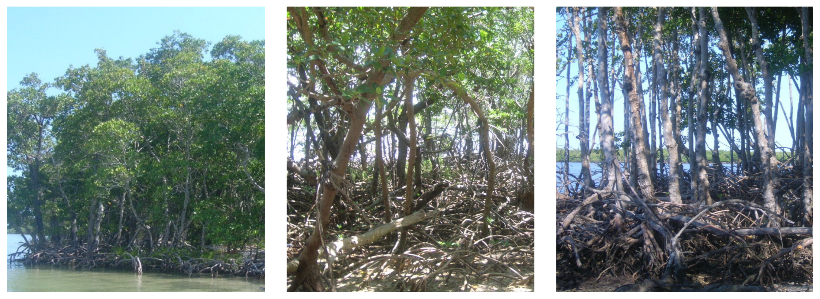
2.1. Research Setting

The Ten Thousand Islands National Wildlife Refuge in southwestern Florida USA (Figure 1) has extensive mangrove stands on many of its densely vegetated islands, which are classified as keys. Three sites were selected based on accessibility by boat and possession of representative characteristics of mangroves. These sites are known by the local names Coon Key, Panther Key, and an unnamed island just east of Panther Key. The sites were given the short code names of CKEY, PKEY, and IEPK, respectively, for identification purposes within the study.

All three sites were dominated by red mangroves (Rhizophora mangle) recognizable by their dense characteristic prop roots, as shown in Figure 2. There was also a limited presence of black mangroves (Avicennia germinans) with their vertical pneumatophores at the upland fringe of the IEPK site. The mangrove stands at all three sites had a canopy height of approximately 9–10 m and average density of approximately 1 trunk per 2–3 square meters (0.3–0.5 trunks/m²). The stands are intertidal, with the aerial root base submerged at the outer fringes of the stands, while the interior portions are only inundated during high tide.

2.2. Field Determination of Manning’s n

Manning’s n bottom friction coefficients were determined in the field using the method and tables from Arcement and Schneider [38]. This method relies on characterizing the contributions of a variety of factors to the overall bottom friction coefficient for the site. The values for these factors, described in the paragraph below, are aggregated as shown in Equation (1):

$$n=\left(n_b+n_1+n_2+n_3+n_4\right)m$$

(1)

Two field researchers experienced in the technique (including the author) assessed each mangrove site for these factors. In situ observations were compared with written descriptions of typical conditions associated with specific value ranges for each factor obtained from “Table 3. Adjustment Values for Factors that Affect the Roughness of a Floodplains [sic]”, an excerpt of which is included as

Table A1. Recreation of Table 3 from Arcement and Schneider, 1989. Minor punctuation errors have been corrected.

Flood-Plain Conditions	n Value Adjustment	Example
Degree of Irregularity (n1)
Smooth	0.000	Compares to the smoothest, flattest flood-plain attainable in a given bed material.
Minor	0.001–0.005	Is a Flood Plain Slightly irregular in shape. A few rises and dips or sloughs may be more visible on the flood plain.
Moderate	0.006–0.010	Has more rises and dips. Sloughs and hummocks may occur.
Severe	0.011–0.020	Flood Plain very irregular in shape. Many rises and dips or sloughs are visible. Irregular ground surfaces in pasture land and furrows perpendicular to the flow are also included.
Variation of Flood-Plain cross section (n2)
Gradual	0.0	Not applicable
Effect of obstruction (n3)
Negligible	0.000–0.004	Few scattered obstructions, which include debris deposits, stumps, exposed roots, logs, piers, or isolated boulders, that occupy less than 5 percent of the cross-sectional area.
Minor	0.005–0.019 *	Obstructions occupy less than 15 percent of the cross-sectional area.
Appreciable	0.020–0.030	Obstructions occupy from 15 percent to 50 percent of the cross-sectional area.
Amount of vegetation (n4)
Small	0.001–0.010	Dense growths of flexible turf grass, such as Bermuda, or weeds growingwhere the average depth of flow is at least two times the height of the vegetation; supple tree seedlings such as willow, cottonwood, arrow-weed, or saltcedar growing where the average depth of flow is at least three times the height of the vegetation.
Medium	0.010–0.025	Turf grass growing where the average depth of flow is from one to two times the height of the vegetation; moderately dense stemy grass, weeds, or tree seedlings growing where the average depth of flow is from two to three times the height of the vegetation; brushy, moderately dense vegetation, similar to 1-to-2-year-old willow trees in the dormant season.
Large	0.025–0.050	Turf grass growing where the average depth of flow is about equal to the height of the vegetation; 8-to-10-years-old willow or cottonwood trees intergrow with some weeds and brush (none of the vegetation in foliage) where the hydraulic radius exceeds 0.607 m; or mature row crops such as small vegetables, or mature field crops where depth flow is at least twice the height of the vegetation.
Very Large	0.050–0.100	Turf grass growing where the average depth of flow is less than half the height of the vegetation; or moderate to dense brush, or heavy stand of timber with few down trees and little undergrowth where depth of flow is below branches, or mature field crops where depth of flow is less than the height of the vegetation.
Extreme	0.100–0.200	Dense bushy willow, mesquite, and saltcedar (all vegetation in full foliage), or heavy stand of timber, few down trees, depth of reaching branches.
Degree of Meander (m)
	1.0	Not Applicable

* The range of values for the minor condition of n₃ contained a typographical error in the original publication. The correct range is shown here.

in Appendix A, and photographic examples presented in Section 3 of Arcement and Schneider [38]. Due to the age of the original publication and the low image resolution, a photographic example from Section 3 of Arcement and Schneider [38] could not be provided in Appendix A.

Each researcher independently estimated values for each factor, as described below, and the values were averaged. These observations were constrained to the zone within 1 m of the ground elevation:

• Degree of irregularity (n₁). This factor was assessed by carefully walking through the site core and qualitatively assessing the microtopographic variation or rugosity contributed by depressions and/or mounds with areas of approximately 1 m² or less.
• Effect of obstruction (n₃). The researchers viewed the site core from multiple external positions and estimated the percentage of vertical cross-sectional area occupied by non-vegetative or non-living vegetative debris such as boulders, fallen logs, and garbage.
• Amount of vegetation (n₄). Like n₃, the researchers viewed the site core from multiple external positions and estimated the percentage of vertical cross-sectional area occupied by living vegetation.

Note that the factor n₂ represents the effect of channel cross-section variation; therefore, it is not applicable to the determination of Manning’s n for a floodplain. Similarly, the factor m represents the degree of meandering of the channel and is also not applicable to floodplains [38]. A shallow (less than 10 cm deep) soil sample of approximately 2 kg was excavated from the ground surface at each site to calculate the contribution of the ground surface, termed the base factor (n_b), to the overall Manning’s n for the site. The soil sample was oven dried, and a sieve analysis was performed to determine the 84th percentile particle diameter (d₈₄). This d₈₄ value was used in Equation (2) to determine n_b.

$$n_b=\frac{\left(0.8204\right)R^{1/6}}{1.16+2.0\hspace{0.17em}\log \left(\frac{R}{d_{84}}\right)}$$

(2)

The remaining variable in Equation (2), R, is the hydraulic radius of the flow, which is equal to the cross-sectional flow area divided by the wetted perimeter. For broad floodplains, R converges to the depth of flow since the horizontal dimension is much greater than the depth [38]. Thus, for floodplains, R is assumed to be equal to the depth of flooding in meters (for the units used here). Since depth is a dynamically computed result in the storm surge model, it varies throughout the simulation. For the purposes of this work, a value of 1 m was chosen to align with the existing training data for the random forest parameter estimation model (referred to hereafter as the RF model) [34].

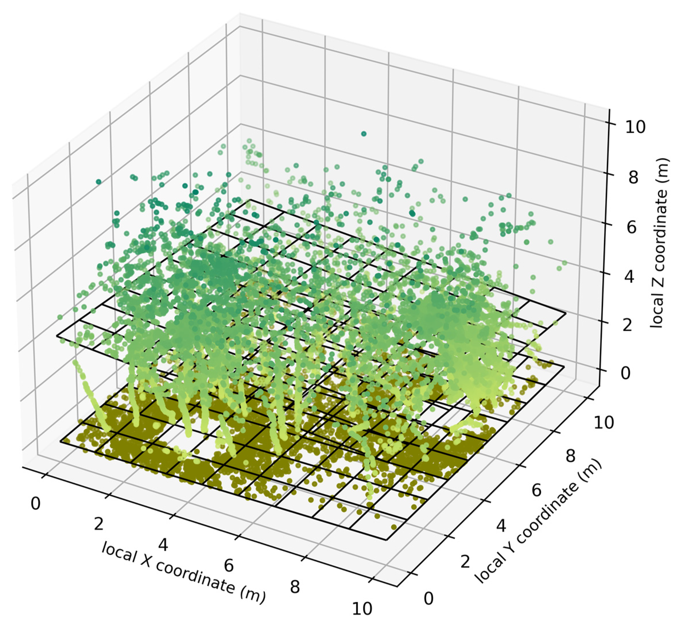
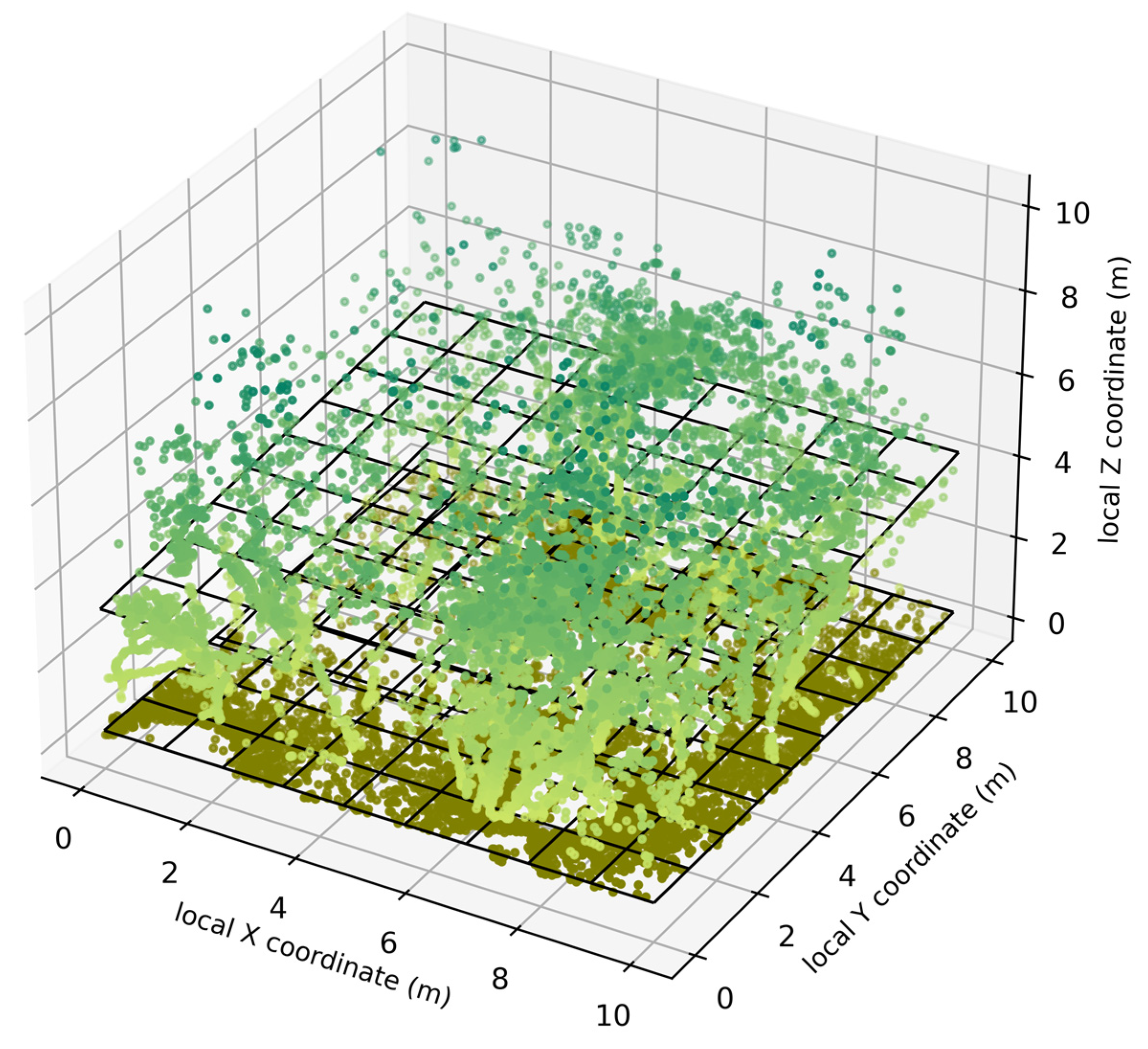
2.3. Laser Scanning Data Acquisition and Processing

The point cloud data for this project were acquired by TLS. Once the data were exported from the equipment vendor’s software, all point cloud processing tasks were completed using the Point Data Abstraction Library (PDAL) command line and Python tools [39,40]. Point cloud information and details on the processing steps, including cropping, classification, and calculation of height above ground, are presented below.

In 2015, a FARO Focus 3d S120 terrestrial laser scanner was used to acquire point clouds for three mangrove stands in the Ten Thousand Islands National Wildlife Refuge in southwestern Florida. Due to the dense, twisting, and stiff characteristics of this type of vegetation, from five to eight scan positions were used, with five 200 mm white spherical targets deployed to aid in registration of the individual scans on a site. The scans were processed using the FARO’s SCENE software version 2018.0 to register (combine) the scans and delete the targets. It is important to note that, at this point in the processing pipeline, the points are referenced to a local scanner-centric coordinate system and are not georeferenced to a recognized datum and coordinate projection.

A 10 m by 10 m central core of each mangrove stand was extracted from the point cloud and its coordinates were shifted so that the minimum x, y, and z values were zero. These points were classified into ground and non-ground points using PDAL Simple Morphological Filter (smrf) [41]. The “max_window_size” and “cell_size parameters” were set to 1.0 m and 0.1 m, respectively, to facilitate processing of these relatively small areas [41]. The height above ground (HAG) was then calculated using PDAL HAG nearest neighbor (hag_nn) with the default parameters. This core point cloud contained the data that were used to parameterize surface roughness.

2.4. Determination of Aerodynamic Roughness Length from TLS

In order to calculate aerodynamic roughness length from the three-dimensional TLS point cloud, an adaptation of the method presented by Lettau [42] was used. This method is based on the following equation:

$$z_0=0.5H\frac{S}{A}$$

(3)

where H (m) is the average height of the above-ground obstacles, S (m²) is the average vertical silhouette area of the obstacles, and A (m²) is the average plan view area occupied by the obstacles. To capitalize on the dense TLS point cloud, Equation (3) was modified from an area to a volumetric context by subdividing the TLS point cloud into 1 m³ voxels, calculating various values that are analogous to H, S, and A in Equation (3), and aggregating the results. The analogous values for the volumetric method will be given a star superscript in the description below.

First, the TLS point cloud was subdivided into n voxels of equal dimension, in this case 1 m³. The total site volume, V, was calculated by summing the voxel volumes (Equation (4)); this value is analogous to the site area A in Equation (3). The number of points in each voxel were counted to produce values $p_1\dots p_n$. The volume fraction of each pixel was calculated as shown in Equation (5). The P₅₀ value represented the median number of points in all voxels that contain points. Voxels that contain P₅₀ points or greater were considered “full” and received a volume fraction value of 1.0. The volume fraction of each pixel was then multiplied by the voxel volume, as shown in Equation (6), to obtain the point volume for each voxel $v_i$. All $v_i$ values were then summed using Equation (7) to obtain the point volume for the site, which serves as an analog for S in Equation (3) Finally, the maximum point heights above ground were selected using a 1 m moving window approach with no overlap. The average obstacle height for the site was determined by calculating the mean maximum point height above ground $h_i$ from each of the m moving windows, as shown in Equation (8); this value is analogous to H in Equation (3).

$$A^{*}=V$$

(4)

$$f_i=\min \left(\frac{p_i}{P_{50}},1.0\right)$$

(5)

$$v_i=\left(f_i\right)\left(1\hspace{0.17em}{m}^3\right)$$

(6)

$$S^{*}={\displaystyle \sum _{i=1}^n{v}_i}$$

(7)

$$H^{*}=\frac{{\displaystyle \sum _{i=1}^m{h}_i}}{m}$$

(8)

With values for H*, S*, and A*, the aerodynamic roughness length was calculated for each site using Equation (3). The density of the point cloud is dependent on the data acquisition process, with more scan positions generating more points, so the 10 m by 10 m core of the TLS point cloud for each site was thinned by random sampling to 30,000,000 points or a density of 300,000 ppsm to enhance comparability across the three sites. Further, to test the sensitivity of the method to the density of the point cloud, fractions of the TLS data were randomly sampled, without replacement, at 10 levels from 1.0 (all points) to 0.01 (1 % of the points). At each thinning level, 10 replicate samples were taken except for the 1.0 level, which contains all 30,000,000 points.

2.5. Random Forest Technique for Surface Roughness Parameter Estimation

The RF model used here was developed by Medeiros et al. [34] and utilizes statistics mined from a point cloud as predictor variables. This method requires that the point cloud is classified into ground and non-ground points and that the non-ground points have a calculated height above ground value. Point clouds of this configuration are typically referred to as “xyzch” to indicate the five fields in the dataset. Only a brief summary of the required data is presented here; for additional details, we refer the reader to the original publication [34].

The RF model requires three predictor variables mined from the point cloud: non-ground point height variance (σ_NG), ground point elevation variance (σ_G), and the height of the non-ground point regression plane (H_NG). After computing the predictor variables from the TLS point clouds for the three mangrove areas and coupling them with the field measured Manning’s n and z₀, they were appended to the training data. Due to the small number of records in the data set (28 sites including the mangroves), a leave-one-out cross-validation (LOOCV) procedure was carried out using the Python module scikit-learn. This process involves removing one record from the dataset, training the random forest on the remaining data, using that trained model to predict the target values for the held-out record, and repeating the cycle for every record in the dataset. LOOCV has been used in numerous applications of machine learning regression techniques to environmental studies, where the ground-truth data acquisition involves extensive field work [43,44,45] and thus produces small (by typical machine learning standards) training data sets. A bootstrapping validation method was not chosen since the RF algorithm itself relies heavily on bootstrapping when building the decision trees comprising the random forest.

The hyperparameters of the RF model were chosen using a grid search optimization method in scikit-learn. The domains for the grid search were a range of discrete, typical values for RF models and are shown in parentheses. The “max_depth” parameter (3, 4, 5) constrains the number of splits in each decision tree in the random forest. The “max_features” parameter (0.3, 0.6, 0.9, “sqrt”, “log2”, “None”) establishes the number of features in the randomly chosen subset of features that can be considered when determining the best split at each level of the decision tree by specifying either the fraction of possible features or the calculation method for determining the number of features. “Sqrt” chooses a number of features that is equal to the square root of the total number of features. “Log2” uses the base 2 logarithm in a similar way. “None” considers all possible features at every split. The “min_samples_leaf” (1, 2, 3) specifies the number of samples at the terminal nodes of each decision tree. If this parameter is greater than one, the values that remain in the leaf node are averaged to form the predicted value. When this parameter is greater than one, it tends to smooth out the prediction field since the predictions from each tree are not strictly constrained to the label values. Lastly, the “n_estimators” parameter (51, 101, 201, 401, 801, 1601) specifies the number of trees in the random forest. The results of the grid search are shown in

Table 1. Random Forest parameter estimation model hyperparameters.

RF Model	Max_Depth	Max_Features	Min_Samples_Leaf	n_Estimators
Manning’s n	5	0.3	2	1601
z0	3	0.3	2	1601

. The only other RF model parameter was the arbitrary “random_state” variable, which was implemented consistently across all computations for reproducibility.

Since the TLS data are much more dense than typical ALS data, the TLS point cloud was randomly sampled from its native density of from ~300 k ppsm to 200 ppsm before calculating the predictor variables used in the RF model. Thirty replicate samples were processed in this way and the mean value for each predictor variable was incorporated into the training data for future use. Lastly, to investigate the sensitivity of the Manning’s n and z₀ predictions to the field measurements, the labels on the data (i.e., the field measured n and z₀) were perturbed by selecting 30 replicate samples from a gaussian distribution with a mean of the measured value and a standard deviation of 50% of the mean value. These were used to produce the uncertainty bands of one standard deviation around the prediction residuals.

3. Results

The results achieved in this study are presented in this section, beginning with the field-measured values for Manning’s n and followed by the TLS-measured aerodynamic roughness length, z₀. The final part of this section will present the LOOCV results of the expanded RF model data set. These results will be put into context in the Discussion and Conclusions section, which will also include a description of their limitations, implications, and recommended future work.

3.1. Field Measured Manning’s n Values

Manning’s n bottom friction coefficient was measured in the field for each of the three mangrove sites. The values for each factor and the overall Manning’s n value are presented in

Table 2. Manning’s n based on factors measured in the field and laboratory.

Site	d84 (mm)	nb	n1	n3	n4	n
CKEY	3.51	0.019	0.005	0.025	0.074	0.123
IEPK	16.2	0.024	0.007	0.029	0.053	0.113
PKEY	12.8	0.023	0.006	0.030	0.088	0.147

.

The mean value for the Manning’s n bottom friction coefficient across all three sites is 0.128, with a standard deviation of 0.014. Relative to the magnitude of typical Manning’s n values, the standard deviation indicates that there is considerable variability in this parameter for mangroves across southwest Florida.

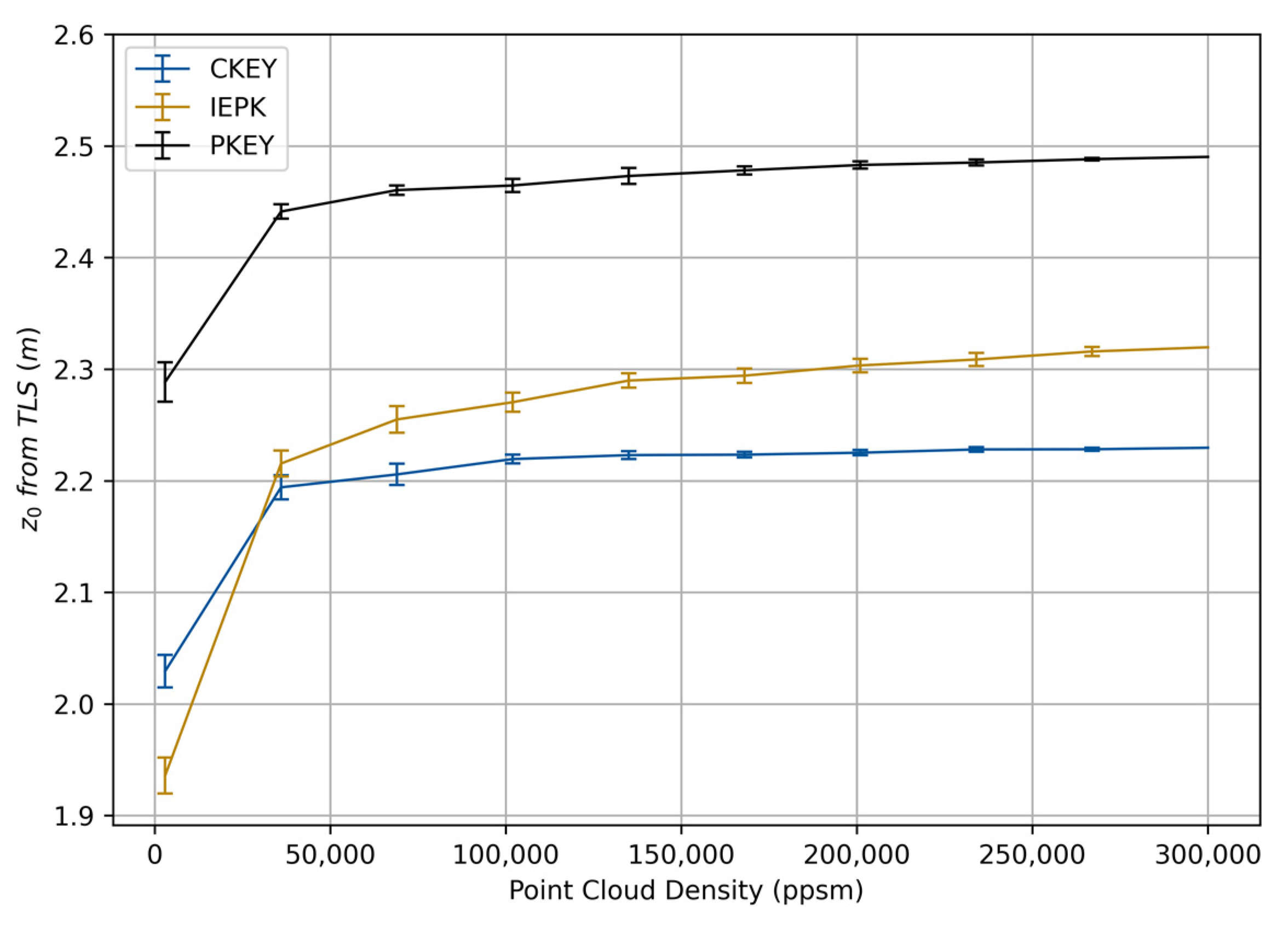
3.2. Aerodynamic Roughness Length Measured from TLS Data

The z₀ values were measured using a voxel-based point cloud processing method presented in this paper for each of the mangrove sites. The values for each factor in Equation (3), modified according to the proposed method and calculated using a 300,000 ppsm TLS point cloud for each site, are shown in

Table 3. Aerodynamic roughness length z₀ measured from the TLS point cloud.

Site	H* (m)	S* (m3)	A* (m3)	z0 (m)
CKEY	8.60	571	1100	2.23
IEPK	10.9	637	1500	2.31
PKEY	9.01	606	1100	2.48

.

The mean value for z₀ across all three mangrove sites is 2.34 m with a standard deviation of 0.01. This indicates that the aerodynamic roughness length is relatively consistent for mangroves in southwest Florida.

The sensitivity of z₀ to the point cloud density is depicted in Figure 3. As shown, the z₀ value converges as point cloud density increases. The error bars indicate that the uncertainty in the result also generally decreases as point cloud density increases.

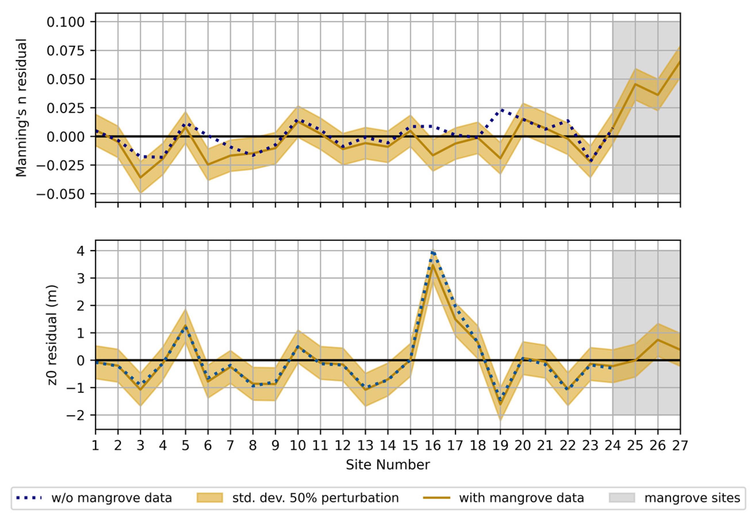
3.3. Leave-One-Out Cross-Validation of Expanded Random Forest Parameter Estimation Model

As stated in Section 2.5, the TLS point clouds for each mangrove site were randomly sampled down to 20,000 points (200 ppsm). The point cloud statistics used as predictor variables in the random forest parameter estimation model were derived from the down-sampled point clouds and are shown in

Table 4. TLS point cloud statistics and associated surface roughness parameters.

Site	σG(m)	σNG(m)	HNG (m)	n	z0(m)
CKEY	0.162	1.607	3.214	0.123	2.23
IEPK	0.231	2.077	4.193	0.113	2.31
PKEY	0.170	1.765	3.368	0.147	2.48

. The features and labels from the existing training data set are omitted for brevity although the Manning’s n values ranged from 0.013 (parking lot) to 0.061 (evergreen forest with shrub/grass understory)) and the z₀ values ranged from 0.00 m (parking lot) to 4.66 m (palustrine forested wetland) [34].

The point clouds, along with the ground and non-ground OLS regression planes, are shown in Figure 4 (CKEY), Figure 5 (IEPK), and Figure 6 (PKEY). Factors that contribute to both surface roughness parameters including variability in the point heights, the density of mangrove trunks, the presence of prop roots, and the overall canopy height are all visible in the three figures.

The LOOCV prediction residuals for the RF model are shown in Figure 7. The results are presented in this manner to align with the original random forest parameter estimation model paper [34] for comparison. The residuals for Manning’s n appear to be slightly larger (worse) when the new mangrove sites are included in the training data. The residuals for Manning’s n of the mangrove sites themselves were larger than those for the sites in the original data. This is likely attributed to the Manning’s n values for mangroves being the highest values in the new training data set; therefore, it is plausible that the RF model would underpredict their values (resulting in larger positive residuals). The width of the uncertainty band around the predictions with mangrove sites included indicates that the RF model was sensitive to the 50% perturbations in the field-measured Manning’s n.

For z₀, the predictions with or without the mangrove sites in the training data were essentially the same. Furthermore, the relatively narrow uncertainty band indicates that for z₀, the random forest parameter estimation model was more robust against perturbation in the field-measured z₀ values. The z₀ residuals for the mangrove sites were generally smaller (more accurate) than those for the original training data set.

To enable further comparison, the prediction accuracy metrics for both versions of the RF model are shown in

Table 5. Random Forest parameter estimation model prediction accuracy metrics.

Model	MAE (m)	RMSE (m)	R2
n w/o mangrove sites	0.010	0.012	0.086
n with mangrove sites	0.016	0.022	0.516
z0 w/o mangrove sites	0.730	1.121	0.009
z0 with mangrove sites	0.664	0.984	0.310

.

The residual-based metrics MAE and RMSE for Manning’s n were both weakened by the inclusion of the mangrove sites into the training data. The same metrics for z₀ were improved. For both surface roughness parameters, the R² values were substantially improved, going from essentially no correlation to a moderate correlation. Overall, the inclusion of the mangrove sites produced mixed results when assessed against the assumption that the addition of new data, especially when the new data expand the range of values for the predicted quantity, will improve the performance of a machine learning regression model.

4. Discussion

Mangroves are a dominant land cover in many of the hurricane prone regions of the western Atlantic; therefore, parameterizing them accurately in coastal storm surge and compound flooding models is essential. Furthermore, they are actively expanding northward, especially along Florida’s east and the Gulf of Mexico coasts, so their impact on coastal resilience will increase correspondingly [46,47].

The field measured values for Manning’s n and z₀ are generally aligned with other values for mangroves in the literature, as shown in

Table 6. Mangrove Manning’s n values from the literature.

Publication	n
Wolanski et al., 1980 [48]	0.2–0.4
Liu et al., 2003 [49]	0.045–0.281
Urish et al., 2009 [50]	0.084–0.445
Zhang et al., 2012 [4]	0.15

, although they appear to be in the lower part of the range. This agrees with the residuals shown in Figure 7, as the Manning’s n values for the mangrove sites were consistently underpredicted (i.e., produced a positive residual when calculating true minus predicted Manning’s n). One reason for this may be that the lower end of the range from the literature refers to areas that are emergent swamps and marshes, and thus usually contain water, lowering their effective bottom friction coefficient. The root structures of the mangroves measured in this study were submerged only at the fringes, while the inner core of the stands was dry at high tide.

At the time of publication, no other field-measured values for z₀ in mangroves could be found. However, when mangrove z₀ values were necessary for a storm surge modeling study, researchers tended to use z₀ values from other, seemingly similar, LULC classes as a proxy for mangroves. For example, in 2016, Deb and Ferreira used woody wetlands, a National Land Cover Dataset (NLCD) classification [51], to parameterize surface roughness for mangroves [52]. This resulted in a Manning’s n of 0.100 and a z₀ of 0.550 m, following the precedents set by Mattocks and Forbes [53], Bunya et al. [22], and Atkinson et al. [23]. Using that same logic, the value of 0.128 measured in this study would correspond approximately to wetland forest–deciduous [22]. However, more recent work utilizing typical three-dimensional structural characteristics of mangroves idealized into cylindrical shapes, coupled with a porosity-based approach, suggests that the wind speed reduction capacity of mangrove forests is more significant than previously thought [54]. This may be attributed to mangrove stands having greater canopy heights than typical areas classified as woody wetlands. The mangroves measured for this study had an average canopy height of 9.85 m, while areas classified as woody wetlands have an average height of approximately 7 m [55]. Based on this information, the values of 0.128 for Manning’s n and 2.34 m for z₀ are reasonable and recommended for use in southwest Florida. However, an even more robust recommendation would be to compute z₀ across the model domain using publicly available ALS data and the voxel-based method presented herein.

In Figure 3, it appears that a point cloud density of approximately 30,000 ppsm effectively achieves the true result; however, this is still multiple orders of magnitude more dense than typical ALS point clouds, which would be the preferred data source for mapping at the regional scale. This would more accurately represent the spatial variability of z₀ in the region but may underestimate z₀ in many locations. Future work will involve the development of an analogous procedure for Manning’s n based on ALS data coupled with published soil maps. The results from this future work could lessen the reliance on the machine learning methods, such as the RF model used here, which suffer from small training data sets. Figure 3 indicates that the voxel-based method is sensitive to the point cloud density, which can vary across an ALS collection area, so this would need to be investigated further prior to deployment of the method across a regional model domain where ALS (5–200 ppsm) data would be the source.

In addition to the sensitivity to point cloud density, the calculation of z₀ may also be sensitive to the one cubic meter voxel size and the one square meter window size for determining S* and H*, respectively. Reducing those sizes would increase the resolution of the spatial discretization of the point cloud and may improve the representation of smaller features like tall grass, shrubs, or prop roots. The influence of this decision would likely be more pronounced closer to the ground surface. At the 1 m resolution presented here, lower voxels were almost always characterized as fully obstructed due to the high number of points reflecting off the mangrove prop roots. Increasing the resolution by making the voxel dimension smaller would result in more empty or partially full voxels, which could change the calculated z₀. If this method is adapted for calculating Manning’s n, as suggested above, this would have to be investigated.

The incorporation of mangrove sites into the RF model produced mixed results. It was expected that the expansion of the training dataset would result in more robust and accurate predictions for both surface roughness parameters, but this was not the case. The prediction accuracy metrics in Table 5 were used to evaluate whether the inclusion of the mangrove sites improved the RF model. When the mangrove sites were included in the training data, the MAE and RMSE values were worse for Manning’s n and better for z₀. In the case of Manning’s n, this would indicate that the predicted values were less accurate. Further, the predicted Manning’s n values for the mangrove sites themselves were among the weakest in the LOOCV process. In contrast, the predicted z₀ values were improved slightly by including the mangrove sites. The z₀ predictions for the mangrove sites themselves were among the strongest in the LOOCV process. The R² metric is significantly improved by including the mangrove sites. The mixed results could be attributed to the tendency of small training datasets to produce significant fluctuations in prediction accuracy as new data are added. In this case, three new sites with essentially the same predictor features and labels were added to the data set, so it is possible that the inclusion of the mangrove sites had the effect of polluting the training data. The incorporation of additional data, especially data which further diversify the range of predictors and labels, could reverse this degradation in predictive capability in Manning’s n. In this work and the original RF model paper, the determination of the field or ground truth Manning’s n is much more subjective than z₀. This may also be a contributing factor to the difference in prediction improvement between the two surface roughness parameters.

As mentioned in the introduction, the long-term objective of this work is to develop frequently updated maps for both Manning’s n and z₀ for use in coastal modeling that account for morphological changes due to sea level rise, storm damage, and other drivers of land cover change. These maps can be produced and updated as new ALS data are acquired, thus reflecting the synoptic conditions at many points in the past. This will allow for modelers to hindcast past storms as accurately as possible by using the conditions that were present at the time. If the voxel-based method for determining z₀ from point cloud data could be adapted for Manning’s n, the subjectivity inherent in determining ground truth Manning’s n values could be eliminated. This would also mitigate the persistent problem of spatial auto-correlation [56] in broad-scale environmental attribute maps based on predictions from machine learning models validated with LOOCV [57]. In the work presented here, the LOOCV results should be interpreted as further evidence that the RF model, and by extension other similra machine learning-based models, should be used with caution when they are trained with limited ground-truth data, especially those containing subjective estimates of factors.

5. Conclusions

This study was focused on the determination of two surface roughness parameters for mangroves in southwestern Florida, USA. The Manning’s n hydraulic bottom friction coefficient and the aerodynamic roughness length, z₀, were measured in the field at three sites in the 10,000 Islands National Wildlife Refuge dominated by black mangroves (Avicennia germinans). Manning’s n was measured using the method of Arcement and Schneider [38], where field personnel estimate the individual contributing factors and aggregate them to form the overall Manning’s n. The mean Manning’s n value was 0.128, which aligns with the lower end of the ranges found in the literature. Aerodynamic roughness length was calculated using a novel three-dimensional voxel-based method presented herein, which derives vegetation density and height measurements from a terrestrial laser scanning point cloud. The mean measured value for z₀ was 2.34 m. The literature on the use of this parameter specifically for mangroves is sparse; however, the value does generally align with the upper range of values from similar land cover classes used as proxies for mangroves in previous storm surge studies. These values are recommended for use in mangrove areas in coastal flooding studies that utilize spatially distributed hydraulic bottom friction coefficients and wind reduction parameters.

This study also utilized the field measured surface roughness parameters to augment the training data and test a previously developed random forest regression model that predicts Manning’s n and z₀ based on statistics derived from the classified (ground and non-ground) point cloud. The incorporation of the mangrove surface roughness parameters weakened the predictions for Manning’s n and improved the predictions for z₀; therefore, the overall impact of the mangrove sites was inconclusive. The mixed results were primarily attributed to the small training data set (28 records including the mangrove sites) and the associated sensitivity of machine-learning-based models to prediction targets containing subjective estimates. Since the use of machine learning to determine environmental characteristics like surface roughness involves extensive field work to collect ground-truth data, small datasets are common. To address this, future work should focus on developing deterministic methods, like the point cloud analysis method for z₀ presented here, for calculating Manning’s n, thus reducing the dependence on subjective estimates.

References

1. Montgomery, J.M.; Bryan, K.R.; Mullarney, J.C.; Horstman, E.M. Attenuation of Storm Surges by Coastal Mangroves. Geophys. Res. Lett. 2019, 46, 2680–2689. [Google Scholar] [CrossRef]
2. Dasgupta, S.; Islam, S.; Huq, M.; Khan, Z.H.; Hasib, R. Quantifying the protective capacity of mangroves from storm surges in coastal Bangladesh. PLoS ONE 2019, 14, e0214079. [Google Scholar] [CrossRef] [PubMed]
3. Liu, H.; Zhang, K.; Li, Y.; Xie, L. Numerical study of the sensitivity of mangroves in reducing storm surge and flooding to hurricane characteristics in southern Florida. Cont. Shelf Res. 2013, 64, 51–65. [Google Scholar] [CrossRef]
4. Zhang, K.; Liu, H.; Li, Y.; Xu, H.; Shen, J.; Rhome, J.; Smith, T.J. The role of mangroves in attenuating storm surges. Estuar. Coast. Shelf Sci. 2012, 102–103, 11–23. [Google Scholar] [CrossRef]
5. Blankespoor, B.; Dasgupta, S.; Lange, G.-M. Mangroves as a protection from storm surges in a changing climate. Ambio 2017, 46, 478–491. [Google Scholar] [CrossRef]
6. Smith, T.J.; Anderson, G.H.; Balentine, K.; Tiling, G.; Ward, G.A.; Whelan, K.R.T. Cumulative impacts of hurricanes on Florida mangrove ecosystems: Sediment deposition, storm surges and vegetation. Wetlands 2009, 29, 24–34. [Google Scholar] [CrossRef]
7. Lagomasino, D.; Fatoyinbo, T.; Castañeda-Moya, E.; Cook, B.D.; Montesano, P.M.; Neigh, C.S.R.; Corp, L.A.; Ott, L.E.; Chavez, S.; Morton, D.C. Storm surge and ponding explain mangrove dieback in southwest Florida following Hurricane Irma. Nat. Commun. 2021, 12, 4003. [Google Scholar] [CrossRef]
8. Luettich, R.A.; Westerink, J.J.; Scheffner, N.W. ADCIRC: An Advanced Three-Dimensional Circulation Model for Shelves, Coasts, and Estuaries, Report 1: Theory and Methodology of ADCIRC-2DDI and ADCIRC-3DL; Department of the Army, US Army Corps of Engineers, Waterways Experiment Station: Vicksburg, MS, USA, 1992; pp. 1–137. [Google Scholar]
9. Luettich, R.; Westerink, J. Formulation and Numerical Implementation of the 2D/3D ADCIRC Finite Element Model Version 44. XX; University of North Carolina Rep.: Chapel Hill, NC, USA, 2004; p. 74. [Google Scholar]
10. Dietrich, J.C.; Westerink, J.J.; Kennedy, A.B.; Smith, J.M.; Jensen, R.E.; Zijlema, M.; Holthuijsen, L.H.; Dawson, C.; Luettich, R.A., Jr.; Powell, M.D.; et al. Hurricane Gustav (2008) waves and storm surge: Hindcast, synoptic analysis and validation in southern Louisiana. Mon. Weather Rev. 2011, 139, 2488–2522. [Google Scholar] [CrossRef]
11. Bilskie, M.V.; Hagen, S.C.; Medeiros, S.C.; Cox, A.T.; Salisbury, M.; Coggin, D. Data and numerical analysis of astronomic tides, wind-waves, and hurricane storm surge along the northern Gulf of Mexico. J. Geophys. Res.-Ocean. 2016, 121, 3625–3658. [Google Scholar] [CrossRef]
12. Booij, N.; Ris, R.C.; Holthuijsen, L.H. A third-generation wave model for coastal regions: 1. Model description and validation. J. Geophys. Res. 1999, 104, 7649–7666. [Google Scholar] [CrossRef]
13. Dietrich, J.C.; Zijlema, M.; Westerink, J.J.; Holthuijsen, L.H.; Dawson, C.; Luettich, R.A., Jr.; Jensen, R.E.; Smith, J.M.; Stelling, G.S.; Stone, G.W. Modeling hurricane waves and storm surge using integrally-coupled, scalable computations. Coast. Eng. 2011, 58, 45–65. [Google Scholar] [CrossRef]
14. Straatsma, M. 3D float tracking: In situ floodplain roughness estimation. Hydrol. Process. 2009, 23, 201–212. [Google Scholar] [CrossRef]
15. Straatsma, M.W.; Baptist, M.J. Floodplain roughness parameterization using airborne laser scaning and spectral remote sensing. Remote Sens. Environ. 2008, 112, 1062–1080. [Google Scholar] [CrossRef]
16. Mayo, T.; Butler, T.; Dawson, C.; Hoteit, I. Data assimilation within the Advanced Circulation (ADCIRC) modeling framework for the estimation of Manning’s friction coefficient. Ocean Model. 2014, 76, 43–58. [Google Scholar] [CrossRef]
17. Shields, F.D.; Coulton, K.G.; Nepf, H. Representation of Vegetation in Two-Dimensional Hydrodynamic Models. J. Hydraul. Eng. 2017, 143, 02517002. [Google Scholar] [CrossRef]
18. Werner, M.; Hunter, N.; Bates, P. Identifiability of distributed floodplain roughness values in flood extent estimation. J. Hydrol. 2005, 314, 139–157. [Google Scholar] [CrossRef]
19. Morsy, M.M.; Lerma, N.R.; Shen, Y.; Goodall, J.L.; Huxley, C.; Sadler, J.M.; Voce, D.; O’neil, G.L.; Maghami, I.; Zahura, F.T. Impact of Geospatial Data Enhancements for Regional-Scale 2D Hydrodynamic Flood Modeling: Case Study for the Coastal Plain of Virginia. J. Hydrol. Eng. 2021, 26, 05021002. [Google Scholar] [CrossRef]
20. Warren, I.; Bach, H. MIKE 21: A modelling system for estuaries, coastal waters and seas. Environ. Softw. 1992, 7, 229–240. [Google Scholar] [CrossRef]
21. Makris, C.; Mallios, Z.; Androulidakis, Y.; Krestenitis, Y. CoastFLOOD: A High-Resolution Model for the Simulation of Coastal Inundation Due to Storm Surges. Hydrology 2023, 10, 103. [Google Scholar] [CrossRef]
22. Bunya, S.; Dietrich, J.C.; Westerink, J.J.; Ebersole, B.A.; Smith, J.M.; Atkinson, J.H.; Jensen, R.; Resio, D.T.; Luettich, R.A.; Dawson, C.; et al. A High-Resolution Coupled Riverine flow, Tide, Wind, Wind Wave, and Storm Surge Model for Southern Louisiana and Missippi. Part I: Model Development and Validation. Mon. Weather Rev. 2010, 128, 354–358. [Google Scholar]
23. Atkinson, J.; Roberts, H.; Hagen, S.C.; Zou, S.; Bacopoulos, P.; Medeiros, S.C.; Weishampel, J.F.; Cobell, Z. Deriving frictional parameters and performing historical validation for an ADCIRC storm surge model of the Florida gulf coast. Fla. Watershed J. 2011, 4, 22–27. [Google Scholar]
24. Medeiros, S.C.; Hagen, S.C.; Weishampel, J.F. Comparison of floodplain surface roughness parameters derived from land cover data and field measurements. J. Hydrol. 2012, 452–453, 139–149. [Google Scholar] [CrossRef]
25. Medeiros, S.C.; Ali, T.; Hagen, S.C.; Raiford, J.P. Development of a Seamless Topographic / Bathymetric Digital Terrain Model for Tampa Bay, Florida. Photogramm. Eng. Remote Sens. 2011, 77, 1249–1256. [Google Scholar] [CrossRef]
26. Bilskie, M.V.; Coggin, D.; Hagen, S.C.; Medeiros, S.C. Terrain-driven unstructured mesh development through semi-automatic vertical feature extraction. Adv. Water Resour. 2015, 86, 102–118. [Google Scholar] [CrossRef]
27. Hovenga, P.A.; Wang, D.; Medeiros, S.C.; Hagen, S.C.; Alizad, K. The response of runoff and sediment loading in the Apalachicola River, Florida to climate and land use land cover change. Earth’s Future 2016, 4, 124–142. [Google Scholar] [CrossRef]
28. Alizad, K.; Hagen, S.C.; Medeiros, S.C.; Bilskie, M.V.; Morris, J.T.; Balthis, L.; Buckel, C.A. Dynamic responses and implications to coastal wetlands and the surrounding regions under sea level rise. PLoS ONE 2018, 13, e0205176. [Google Scholar] [CrossRef] [PubMed]
29. Alizad, K.; Hagen, S.C.; Morris, J.T.; Bacopoulos, P.; Bilskie, M.V.; Weishampel, J.F.; Medeiros, S.C. A coupled, two-dimensional hydrodynamic-marsh model with biological feedback. Ecol. Model. 2016, 327, 29–43. [Google Scholar] [CrossRef]
30. Hightower, J.N.; Butterfield, A.C.; Weishampel, J.F. Quantifying Ancient Maya Land Use Legacy Effects on Contemporary Rainforest Canopy Structure. Remote Sens. 2014, 6, 10716–10732. [Google Scholar] [CrossRef]
31. Cannon, D.; Kibler, K.M.; Kitsikoudis, V.; Medeiros, S.C.; Walters, L.J. Variation of mean flow and turbulence characteristics within canopies of restored intertidal oyster reefs as a function of restoration age. Ecol. Eng. 2022, 180, 106678. [Google Scholar] [CrossRef]
32. Cannon, D.J.; Kibler, K.M.; Taye, J.; Medeiros, S.C. Characterizing canopy complexity of natural and restored intertidal oyster reefs (Crassostrea virginica) with a novel laser-scanning method. Restor. Ecol. 2023, 31, e13973. [Google Scholar] [CrossRef]
33. Hooshyar, M.; Kim, S.; Wang, D.; Medeiros, S.C. Wet channel network extraction by integrating LiDAR intensity and elevation data. Water Resour. Res. 2015, 51, 10029–10046. [Google Scholar] [CrossRef]
34. Medeiros, S.C.; Hagen, S.C.; Weishampel, J.F. A random forest model based on lidar and field measurements for parameterizing surface roughness in coastal models. IEEE J. Sel. Top. Appl. Earth Obs. Remote Sens. 2015, 8, 1582–1590. [Google Scholar] [CrossRef]
35. Dorn, H.; Vetter, M.; Höfle, B. GIS-Based Roughness Derivation for Flood Simulations: A Comparison of Orthophotos, LiDAR and Crowdsourced Geodata. Remote Sens. 2014, 6, 1739–1759. [Google Scholar] [CrossRef]
36. Cobby, D.M.; Mason, D.C.; Horritt, M.S.; Bates, P.D. Two-dimensional hydraulic flood modelling using a finite-element mesh decomposed according to vegetation and topographic features derived from airborne scanning laser altimetry. Hydrol. Process. 2003, 17, 1979–2000. [Google Scholar] [CrossRef]
37. Mason, D.C.; Cobby, D.M.; Horritt, M.S.; Bates, P.D. Floodplain friction parameterization in two-dimensional river flood models using vegetation heights derived from airborne scanning laser altimetry. Hydrol. Process. 2003, 17, 1711–1732. [Google Scholar] [CrossRef]
38. Arcement, G.J.; Schneider, V.R. Guide for selecting Manning’s roughness co-efficients for natural channels and flood plains / by George J. Arcement, Jr. and Verne R. Schneider; prepared in cooperation with the U.S. Department of Transportation, Federal Highway Administration. In U.S. Geological Survey Water-Supply Paper; Department of the Interior, U.S. Geological Survey: Denver, CO, USA, 1989; p. 2339, For sale by the Books and Open-File Reports Section, 1989. [Google Scholar]
39. Butler, H.; Chambers, B.; Hartzell, P.; Glennie, C. PDAL: An open source library for the processing and analysis of point clouds. Comput. Geosci. 2021, 148, 104680. [Google Scholar] [CrossRef]
40. PDAL Contributors. PDAL Point Data Abstraction Library. 2022. Available online: https://zenodo.org/records/8436666 (accessed on 22 September 2023).
41. Pingel, T.J.; Clarke, K.C.; McBride, W.A. An improved simple morphological filter for the terrain classification of airborne LIDAR data. ISPRS J. Photogramm. Remote Sens. 2013, 77, 21–30. [Google Scholar] [CrossRef]
42. Lettau, H. Note on Aerodynamic Roughness-Parameter Estimation on the Basis of Roughness-Element Description. J. Appl. Meteorol. 1969, 8, 828–832. [Google Scholar] [CrossRef]
43. Emmanuel, E.D.; Lenhart, C.F.; Weintraub, M.N.; Doro, K.O. Estimating Soil Properties Distribution at a Restored Wetland Using Electromagnetic Imaging and Limited Soil Core Samples. Wetlands 2023, 43, 39. [Google Scholar] [CrossRef]
44. Luo, S.; Wang, C.; Pan, F.; Xi, X.; Li, G.; Nie, S.; Xia, S. Estimation of wetland vegetation height and leaf area index using airborne laser scanning data. Ecol. Indic. 2015, 48, 550–559. [Google Scholar] [CrossRef]
45. Yang, R.-M.; Guo, W.-W. Modelling of soil organic carbon and bulk density in invaded coastal wetlands using Sentinel-1 imagery. Int. J. Appl. Earth Obs. Geoinf. 2019, 82, 101906. [Google Scholar] [CrossRef]
46. Williams, A.A.; Eastman, S.F.; Eash-Loucks, W.E.; Kimball, M.E.; Lehmann, M.L.; Parker, J.D. Record Northernmost Endemic Mangroves on the United States Atlantic Coast with a Note on Latitudinal Migration. Southeast. Nat. 2014, 13, 56–63. [Google Scholar] [CrossRef]
47. Osland, M.J.; Day, R.H.; Hall, C.T.; Feher, L.C.; Armitage, A.R.; Cebrian, J.; Dunton, K.H.; Hughes, A.R.; Kaplan, D.A.; Langston, A.K.; et al. Temperature thresholds for black mangrove (Avicennia germinans) freeze damage, mortality and recovery in North America: Refining tipping points for range expansion in a warming climate. J. Ecol. 2019, 108, 654–665. [Google Scholar] [CrossRef]
48. Wolanski, E.; Jones, M.; Bunt, J. Hydrodynamics of a tidal creek-mangrove swamp system. Mar. Freshw. Res. 1980, 31, 431–450. [Google Scholar] [CrossRef]
49. Liu, W.-C.; Hsu, M.-H.; Wang, C.-F. Modeling of Flow Resistance in Mangrove Swamp at Mouth of Tidal Keelung River, Taiwan. J. Waterw. Port Coast. Ocean Eng. 2003, 129, 86–92. [Google Scholar] [CrossRef]
50. Urish, D.W.; Wright, R.M.; Feller, I.C.; Rodriguez, W. Dynamic Hydrology of a Mangrove Island: Twin Cays, Belize. Smithson. Contrib. Mar. Sci. 2009, 38, 473–490. [Google Scholar]
51. Homer, C.; Dewitz, J.; Fry, J.; Coan, M.; Hossain, N.; Larson, C.; Herold, N.; McKerrow, A.; VanDriel, J.N.; Wickham, J. Completion of the 2001 National Land Cover Database for the Conterminous United States. Photogramm. Eng. Remote Sens. 2007, 73, 337–341. [Google Scholar]
52. Deb, M.; Ferreira, C.M. Simulation of cyclone-induced storm surges in the low-lying delta of Bangladesh using coupled hydrodynamic and wave model (SWAN + ADCIRC). J. Flood Risk Manag. 2016, 11, S750–S765. [Google Scholar] [CrossRef]
53. Mattocks, C.; Forbes, C. A real-time, event-triggered storm surge forecasting system for the state of North Carolina. Ocean Model. 2008, 25, 95–119. [Google Scholar] [CrossRef]
54. Chen, Q.; Li, Y.; Kelly, D.M.; Zhang, K.; Zachry, B.; Rhome, J. Improved modeling of the role of mangroves in storm surge attenuation. Estuar. Coast. Shelf Sci. 2021, 260, 107515. [Google Scholar] [CrossRef]
55. Steyaert, L.T.; Knox, R.G. Reconstructed historical land cover and biophysical parameters for studies of land-atmosphere interactions within the eastern United States. J. Geophys. Res. Atmos. 2008, 113, D02101. [Google Scholar] [CrossRef]
56. Enwright, N.M.; Cheney, W.C.; Evans, K.O.; Thurman, H.R.; Woodrey, M.S.; Fournier, A.M.; Gesch, D.B.; Pitchford, J.L.; Stoker, J.M.; Medeiros, S.C. Elevation-based probabilistic mapping of irregularly flooded wetlands along the northern Gulf of Mexico coast. Remote Sens. Environ. 2023, 287, 113451. [Google Scholar] [CrossRef]
57. Meyer, H.; Pebesma, E. Machine learning-based global maps of ecological variables and the challenge of assessing them. Nat. Commun. 2022, 13, 2208. [Google Scholar] [CrossRef] [PubMed]
Figure 1. Location of field sites Coon Key (CKEY), Panther Key (PKEY), and Island East of Panther Key (IEPK) in the 10,000 Islands National Wildlife Refuge in southwest, FL, USA. Mangrove areas are shaded in pink, ArcGIS map service layer credit: GulfDataAtlas/Mangroves_GOM: National Centers for Environmental Information, NESDIS, NOAA, U.S. Department of Commerce; Office for Coastal Management, NOS, NOAA, U.S. Department of Commerce; National Commission for the Knowledge and Use of Biodiversity (CONABIO). Background image uses ArcGIS map service layer World Imagery converted to grayscale by the author, service layer credit: Esri, DigitalGlobe, GeoEye, i-cubed, USDA FSA, USGS, AEX, Getmapping, Aerogrid, IGN, IGP, swisstopo, and the GIS User Community.
Jmse 11 02053 g001
Figure 2. Photographs of the three mangrove sites in the 10,000 Islands National Wildlife Refuge in southwest, FL, USA. (Left): Coon Key (CKEY), (Center): Panther Key (PKEY), (Right): Island East of Panther Key (IEPK).
Jmse 11 02053 g002
Figure 3. Sensitivity of TLS-derived z0 to point cloud density.
Jmse 11 02053 g003
Figure 4. TLS point cloud and OLS regression planes for CKEY site.
Jmse 11 02053 g004
Figure 5. TLS point cloud and OLS regression planes for IEPK site.
Jmse 11 02053 g005
Figure 6. TLS point cloud and OLS regression planes for PKEY site.
Jmse 11 02053 g006
Figure 7. Residual plots for Manning’s n (top) and z0 (bottom) predicted by the random forest parameter estimation model.
Jmse 11 02053 g007