Article

Theoretical Analysis of Dynamic Response of Pipe Pile with Multi-Defects

1
College of Transportation, Shandong University of Science and Technology, Qingdao 266000, China
2
Cardiff School of Engineering, Cardiff University, Queen’s Buildings, The Parade, Cardiff CF24 3AA, UK
*
Author to whom correspondence should be addressed.
J. Mar. Sci. Eng. 2023, 11(1), 83; https://doi.org/10.3390/jmse11010083
Submission received: 29 November 2022 / Revised: 23 December 2022 / Accepted: 25 December 2022 / Published: 3 January 2023
(This article belongs to the Special Issue Offshore Wind Turbine Foundations)

Abstract

:
A mathematical model for an outer soil, multi-defects pipe pile, and inner soil dynamic interaction system is established to research the influences of multi-defects on the vibration of a pipe pile. The dynamic impedance of the pipe pile is deduced by applying a Laplace transformation method and an impedance recursive technique. Then, the velocity response at the pile head is further obtained using the inverse Fourier transform method. Moreover, parametric analyses are conducted to research the influences of the type, degree, distribution, length, and depth of multi-defects on the vibration of the pipe pile. The results indicate that the characteristics of multi-defects appear different, with amplitude differences and reflected signal features on the velocity admittance and velocity response curve, respectively. This means that the obtained analytical solutions and relevant results can be used to detect multi-defects of pipe piles using the different appearances of the velocity admittance and velocity response curve, as measured in engineering practice.

1. Introduction

Pile, as a reliable foundation to deal with unfavorable geological conditions, has been extensively used in various infrastructures, such as offshore platforms and wind turbines, due to its large capacity. During the construction of the pile foundation, it is inevitable that there is concrete segregation, mud clamping, necking, and other defects, which adversely affect the function of the pile foundation [1,2,3]. However, the detection of pile defects is difficult, due to their invisibility. Therefore, the nondestructive testing method, such as low-strain pile integrity testing (LS-PIT) for the detection of pile defects is crucial to the safety of pile-supported structures. As the cornerstone of LS-PIT, pile–soil dynamic interaction theory has attracted great attention worldwide.
According to the integrity of pile, the existing research for the pile–soil dynamic interaction can be divided into two categories, namely homogeneous pile [4] and defective pile [5]. For the homogeneous pile, relevant studies are mainly aimed at the improvement of the rationality of the mathematical model for pile and soil. The pile analytical models consist of the Euler–Bernoulli model [6,7], the Rayleigh–Love model [8], and the continuum pile model [9]. Among them, the Euler–Bernoulli model is the most commonly used to study the vibration of pile with a large slenderness ratio, due to its simplicity. The development of analytical models for soil includes the simplified Winkler model [10,11,12], the Novak plain strain model [13], and the 3D continuum soil model [14].
However, the LS-PIT technique is intended to detect defects along the pile shaft. Therefore, based on the aforementioned analytical models for pile and soil, many researchers have conducted various theoretical studies for the dynamic interaction of defective pile and soil. Wang et al. [15] researched the vibration of pile with single defect by simplifying the soil as a general Voigt model. Gao et al. [16] generalized the pile defect as Young’s moduli changing, and applied the δ function method to solve the pile dynamic response theoretically. Using the three-dimensional continuum soil model, Wu et al. [17,18] presented a defective pile–soil interaction analytical model for the parallel seismic (PS) method to study the influences of pile defect on wave propagation in soils. Ni et al. [2] used the complex continuous wavelet transform method to analysis the effect of single defect features, such as length and location, on the phase diagram, and gave the corresponding evaluation method for pile defect features. Zheng et al. [19] proposed an impulse response function analysis method to detect the single defect of pile, the accuracy of which was verified by conducting field testing. Considering the various forms of pile single defects, Liu et al. [20] obtained the analytical solutions for the velocity response of pile at multi-points along pile shaft. Compared to the pile with single defect, the dynamic response of multi-defects pile is more complex. Wu et al. [21] applied the Fourier-Hankel integral transform method to derive the analytical solution of the velocity response of multi-defects pile in half-space soil. Yang et al. [22] compared the detection outcomes of different techniques, such as LS-PIT and PS, for pile with multi-defects, by designing large-scale field model testing. For the study of experimental and numerical evaluations of the pile–soil interaction under dynamic loads, Basack Sudip et al. [23] carried out the model experimental for pile groups to study the pile soil interaction under lateral cyclic loading of loose sand, and two alternative numerical models, boundary element model and finite element model (BEM and FEM), were established. Cao et al. [24] proposed a series of field tests of pile groups embedded in multi-layer soil and studied the influence of pile group characteristic parameters on stiffness, dynamic interaction coefficient and dynamic efficiency coefficient in combination with the theoretical model.
The above studies are all carried out for solid pile. In recent decades, a new type of pipe pile, known as cast-in-place concrete pipe pile (PCC), has been widely used to improve the capability and to reduce the settlement of soft ground due to its economy and practicability [25]. For PCC, the existence of inner soil makes its vibration characteristics different from that of solid pile [26]. Zheng et al. [27] investigated the resistance of inner soil to PCC and analyzed the effects of the parameters of inner soil on the response of PCC. Subsequently, Zheng et al. [28,29], Liu et al. [30], Ding et al. [31], and Li et al. [32] adopted different mathematical models for pile and soil to investigate the effects of parameters of PCC and soils on the vertical vibration of PCC. Zheng et al. [33] derived the velocity time history of PCC with a single defect and utilized a parametric analysis to investigate the effect of defect feature on the velocity time history of PCC. Existing research indicates that PCC may have multi-defects due to a cast-in-place process [34]. However, previous analytical models for PCC mainly aimed at the vibration problems of integrity pile or pile with a single defect and are not suitable for multi-defects PCC. Therefore, it is essential to develop an analytical model for multi-defect PCC.
In this study, a mathematical model for an outer soil, multi-defects pipe pile, and inner soil dynamic interaction system is established to research the influence of multi-defects on the vibration of a pipe pile. The dynamic impedance of the pipe pile is deduced by applying a Laplace transformation method and an impedance recursive technique. Then, the velocity response at the pile head is further obtained using the inverse Fourier transform method. Moreover, parametric analyses are conducted to research the influence of the type, degree, distribution, length, and depth of multi-defects on the vibration of the pipe pile.

2. Mathematical Model and Definite Problem

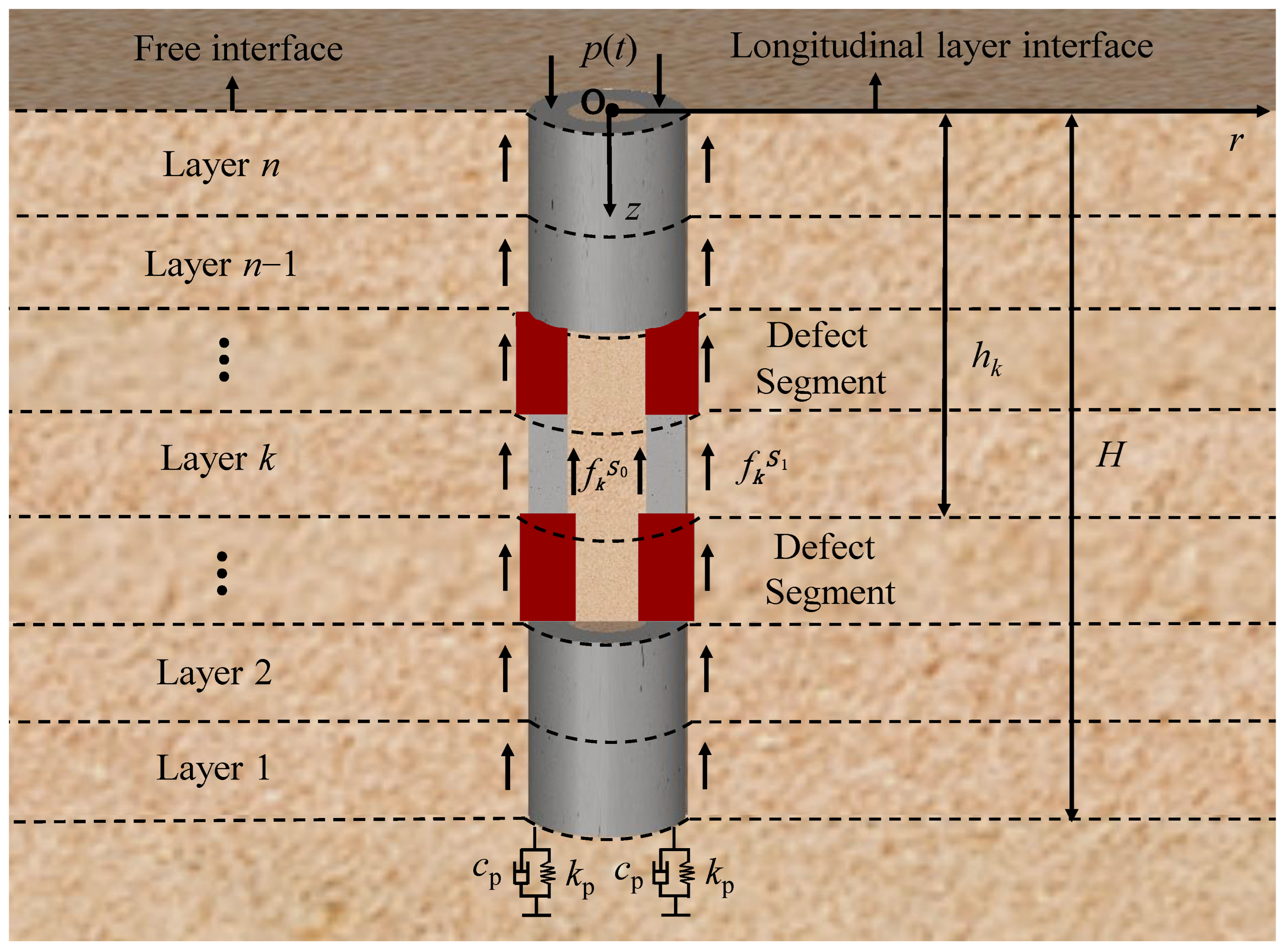
2.1. Simplified Mathematical Model

The simplified mathematical model of a pipe pile–soil dynamic interaction system considering pile with multi-defects is shown in Figure 1. The r and z in the coordinate system represent the radial and vertical variables, respectively. According to the location of a defect within pile, this multi-layered system is numbered 1, 2, …, k, …, n from the pile toe to the head. The length, upper interface depth, inner radius, outer radius, cross section, density, and elastic modulus of the kth pile are lk, hk, r k 0 , r k 1 , S k , ρ k P , and E k P , respectively. According to existing research by Lysmer and Richart [35], the pile end soil behaves similarly to a simply damped oscillator that can be simplified as an analog of a parallel spring and dashpot type. Therefore, the kelvin-voigt model is used to simulate the stiffness and damping at the pile toe. The damping and stiffness coefficients of the visco-elastic support at the pile toe are cp and kp, respectively. The shear modulus, damping coefficient, and density of the kth soil layer are G k 0 ( G k 1 ) , η k 0 ( η k 1 ) , and ρ k 0 ( ρ k 1 ) , respectively. The subscripts k0 and k1 refer to the corresponding parameters for the inner and surrounding soils. f k S 0 and f k S 1 are the shear stresses of the inner and surrounding soils, respectively, at relevant interfaces of the pipe pile. The excitation is p ( t ) . The length of the pipe pile is H.

2.2. Wave Equations

Based on the Novak soil model, the wave equations of the kth pile inner and surrounding soil layers are given as:
G k 0 2 u k S 0 ( r , t ) r 2 + η k 0 3 u k S 0 ( r , t ) t r 2 + G k 0 r u k S 0 ( r , t ) r + η k 0 r 2 u k S 0 ( r , t ) t r = ρ k 0 2 u k S 0 ( r , t ) t 2
G k 1 2 u k S 1 ( r , t ) r 2 + η k 1 3 u k S 1 ( r , t ) t r 2 + G k 1 r u k S 1 ( r , t ) r + η k 1 r 2 u k S 1 ( r , t ) t r = ρ k 1 2 u k S 1 ( r , t ) t 2
where u k S 0 and u k S 1 are the displacements of the kth inner soil and surrounding soil, respectively.
According to the Euler–Bernoulli rod theory, the wave equation of the kth pile is given as:
2 u k P ( z , t ) z 2 2 π r k 0 f k S 0 E k P S k 2 π r k 1 f k S 1 E k P S k = ρ k P E k P 2 u k P ( z , t ) t 2
where u k P is the displacement of the kth pile.

2.3. Boundary Conditions

(1) Pile inner soil:
lim r 0 u k S 0 ( r , t )
The displacement continuity and force balance conditions of pile and inner soil are given as:
u k S 0 ( r k 0 , t ) = u k P ( r k 0 , t )
f k S 0 = τ k S 0 ( r ) | r = r k 0
(2) Pile surrounding soil
When r→∞, the displacement of kth pile surrounding soil is zero.
lim r u k S 1 ( r , t ) = 0
The displacement continuity and force balance conditions of pile and surrounding soil are given as:
u k S 1 ( r k 1 , t ) = u k P ( r k 1 , t )
f k S 1 = τ k 1 S 1 ( r ) | r = r k 1
(3) Pile shaft
E n P S n u n P ( z , t ) z | z = 0 = p ( t )
E 1 P u 1 P ( z , t ) z | z = H = ( k p u 1 P ( z , t ) + c p u 1 P ( z , t ) t )

3. Solutions for Definite Problems

3.1. Solutions for Soils

By utilizing the Laplace Transformation (LT), Equations (1) and (2) can be written as
G k 0 2 U k S 0 ( r , s ) r 2 + η k 0 s 2 U k S 0 ( r , s ) r 2 + G k 0 r U k S 0 ( r , s ) r + η k 0 s r U k S 0 ( r , s ) r = ρ k 0 s 2 U k S 0 ( r , s )
G k 1 2 U k S 1 ( r , s ) r 2 + η k 1 s 2 U k S 1 ( r , s ) r 2 + G k 1 r U k S 1 ( r , s ) r + η k 1 s r U k S 1 ( r , s ) r = ρ k 1 s 2 U k S 1 ( r , s )
where U k S 0 ( r , s ) and U k S 1 ( r , s ) are the LT form of u k S 0 ( r , t ) and u k S 1 ( r , t ) , respectively.
Then, Equations (12) and (13) can be further arranged into the following form:
2 U k S 0 ( r , s ) r 2 + 1 r U k S 0 ( r , s ) r = ( q k S 0 ) 2 U k S 0 ( r , s )
2 U k S 1 ( r , s ) r 2 + 1 r U k S 1 ( r , s ) r = ( q k S 1 ) 2 U k S 1 ( r , s )
where q k S 0 = ρ k 0 s 2 G k 0 + η k 0 s , q k S 1 = ρ k 1 s 2 G k 1 + η k 1 s .
The solutions for Equations (14) and (15) are:
U k S 0 ( r , s ) = A k S 0 K 0 ( q k S 0 r ) + B k S 0 I 0 ( q k S 0 r )
U k S 1 ( r , s ) = A k S 1 K 0 ( q k S 1 r ) + B k S 1 I 0 ( q k S 1 r )
where A k S 0 , B k S 0 , A k S 1 , and B k S 1 are underdetermined coefficients.
Utilizing LT for Equations (4) and (7), and substituting them into Equations (16) and (17) yields:
U k S 0 ( r , s ) = B k S 0 I 0 ( q k S 0 r )
U k S 1 ( r , s ) = A k S 1 K 0 ( q k S 1 r )
Subsequently, the shear stiffness of the pile inner and surrounding soils at the interface with pipe pile can be further obtained as
K K k S 0 = 2 π r k 0 τ k S 0 ( r k 0 ) U k P = 2 π r k 0 ( G k 0 + η k 0 s ) q k S 0 I 1 ( q k S 0 r k 0 ) I 0 ( q k S 0 r k 0 )
K K k S 1 = 2 π r k 1 τ k S 1 ( r k 1 ) U k P = 2 π r k 1 ( G k 1 + η k 1 s ) q k S 1 K 1 ( q k S 1 r k 1 ) K 0 ( q k S 1 r k 1 )
where U k P ( r , s ) is the LT form of u k P ( r , t ) .

3.2. Solutions for Pipe Pile

Utilizing LT for Equation (3) and substituting it into Equations (20) and (21) yields:
2 U k P ( z , s ) z 2 α k 2 U k P ( z , s ) = 0
where α k 2 = K K k S 1 E k P S k K K k S 0 E k P S k + ρ k P E k P s 2 .
The solution of Equation (22) is
U k P ( z , s ) = C k P e α k z / l k + D k P e α k z / l k
where α k = α k l k is a dimensionless eigenvalue. C k P and D k P are underdetermined coefficients.
Therefore, the displacement impedance (DI) of the first pile segment at its lower interface ( z = H ) and upper interface ( z = h 1 ) can be expressed as
Z 0 P | z = H = E 1 P S 1 z U 1 P ( z , s ) | z = H U 1 P ( z , s ) | z = H = E 1 P S 1 α 1 ( C 1 P e α 1 H / l 1 D 1 P e α 1 H / l 1 ) l 1 ( C 1 P e α 1 H / l 1 + D 1 P e α 1 H / l 1 ) = S 1 ( k p + c p s )
Z 1 P | z = h 1 = E 1 P S 1 z U 1 P ( z , s ) | z = h 1 U 1 P ( z , s ) | z = h 1 = E 1 P S 1 α 1 ( C 1 P e α 1 h 1 / l 1 D 1 P e α 1 h 1 / l 1 ) l 1 ( C 1 P e α 1 h 1 / l 1 + D 1 P e α 1 h 1 / l 1 )
By combining Equations (24) and (25), the recursive relation of DI can be given as
Z 1 P = E 1 P S 1 α 1 ( β 1 e α 1 h 1 / l 1 e α 1 h 1 / l 1 ) l 1 ( β 1 e α 1 h 1 / l 1 + e α 1 h 1 / l 1 )
where β 1 = E 1 P S 1 α 1 Z 0 P l 1 E 1 P S 1 α 1 + Z 0 P l 1 e 2 α 1 h 0 / l 1 .
According to the coupling conditions of adjacent pile segments, the DI of the kth pile at its upper interface ( z = h k ) can be obtained using the impedance recursive method.
Z k P = E k P S k α k ( β k e α k h k / l k e α k h k / l k ) l k ( β k e α k h k / l k + e α k h k / l k )
where β k = E k P S k α k Z ( k 1 ) P l k E k P S k α k + Z ( k 1 ) P l k e 2 α k h k 1 / l k .
Consequently, the DI at the pile head can be given as
Z n P | z = h n = 0 = E n P S n α n ( β n 1 ) l n ( β n + 1 ) = E n P S n l n Z n P
where β n = E n P S n α n Z n 1 P l n E n P S n α n + Z n 1 P l n e 2 α n h n 1 / l n . Z n P = α n ( β n 1 ) β n + 1 is a dimensionless DI. Z n P = K r + k K i . K r is the dynamic stiffness. K i is the dynamic damping.
Then, the displacement ( H u ) and velocity ( H v ) in the frequency domain of the pile head can be obtained:
H u = 1 / Z n P = l n ( β n + 1 ) E n P S n α n ( β n 1 )
H v = i ω l n ( β n + 1 ) E n P S n α n ( β n 1 ) = 1 ρ n P S n P V n P H v
H v = i θ t n ( β n + 1 ) α n ( β n 1 )
where H v is the dimensionless velocity admittance. V n P = E n P / ρ n P , θ = ω T c , T c = H / V n P , t n = l n / V n P , t n = t n / T c .
When p ( t ) = Q max sin π T t , the dimensionless velocity response of pile can be given using the inverse Fourier transform for Equation (31).
V v = 1 2 π [ H v π T π 2 T 2 θ 2 ( 1 + e i θ T ) ] e i θ t d θ
where T is the pulse width. T = T / T c .

4. Results and Discussion

The parameters for numerical instances are shown in Table 1.
To study the influences of pile multi-defects on the pile vibration, the pile–soil system is divided into five segments (n = 5). The length and depth of each pile are shown in Table 2.

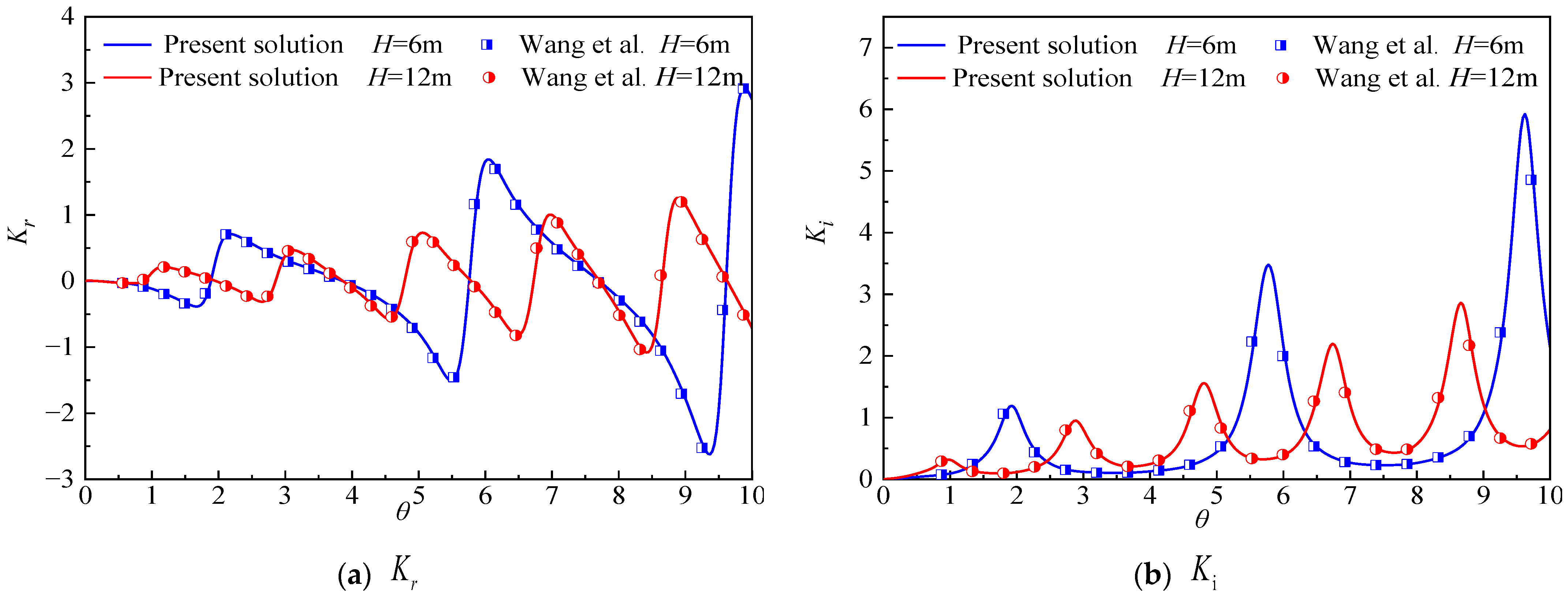
4.1. Verification of the Present Method

To verify the rationality of the present model, the reduction form of the analytical solution of DI expressed in Equation (28) is compared to the existing solution. Wang et al. [36] gives the analytical solution of DI for solid pile. The pipe pile solution is reduced to solid pile by setting r k 0 = 0 and comparing it with the solution of Wang et al. [36] (shown in Figure 2). It is clear from Figure 2 that the present solution agrees well with the existing solutions.

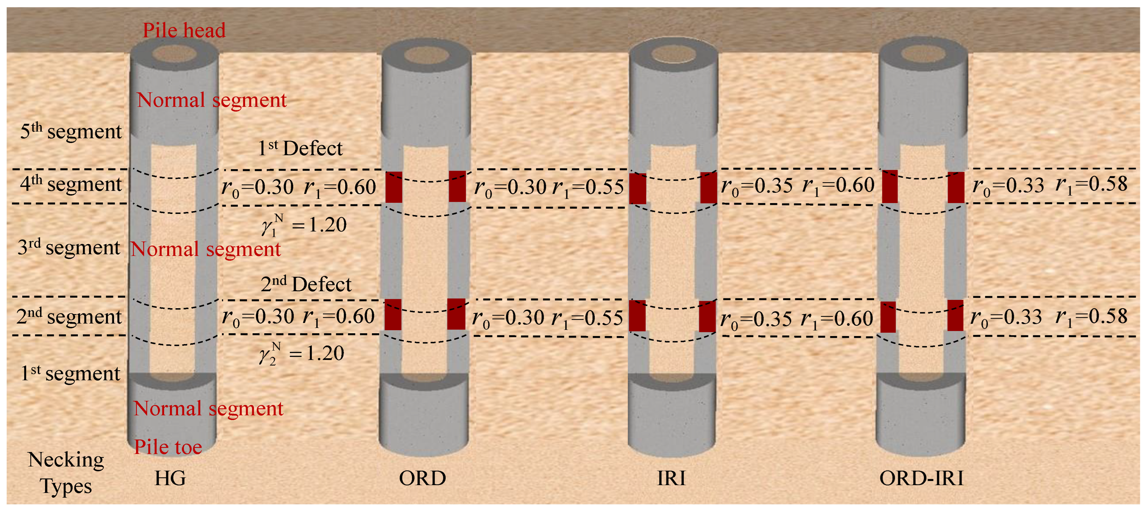
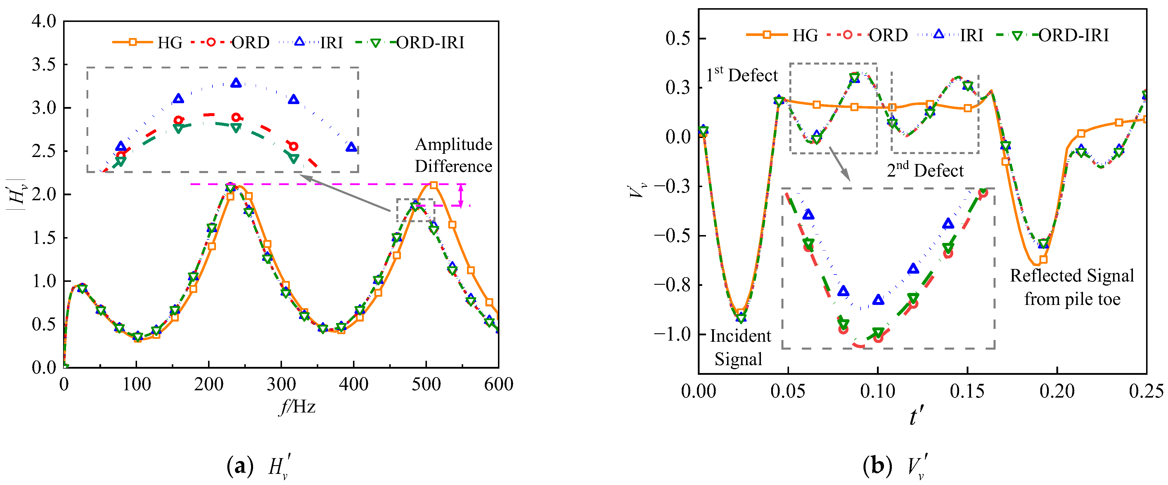
4.2. Effect of Multi-Defects on the Response of the Pipe Pile

To investigate the effect of multi-defect segments along the pipe pile shaft on the response of the pile head, the second and fourth pipe piles are set as defect segments. In the following numerical analysis, the defects are generalized as the changing of the pile section, such as necking and expanding [15]. The defect degree is defined by the ratio of wall thickness for the defect segment to the normal segment.
γ j N = r 1 r 0 r j 1 r j 0
γ j E = r j 1 r j 0 r 1 r 0
where γ j N and γ j E are the defect degrees for necking and expanding, respectively, of the jth defect segment. r j 1 and r j 0 are the outer and inner radii of the jth defect segment. r 1 and r 0 are the outer and inner radii of the normal segment.
The necking defect of pipe pile can be caused by the increase in inner radius or the decrease in the outer radius. Consequently, there are three types for the necking defect, namely the outer radius decrease (ORD), inner radius increase (IRI), and coincidence of ORD and IRI (ORD-IRI). Figure 3 illustrates the diagram of different types of necking defect with the same defect degree. HG refers to the homogeneous pile type. Figure 4 shows the comparison of the pile dynamic response under different necking types.
It can be noticed from Figure 3 and Figure 4 that the amplitude difference (AD) between adjacent crests of admittance for homogeneous pile types can be neglected, while this AD for multi-necking pile is apparent. Specifically, the AD of ORD-IRI is the largest, followed by that of IRI, and that of ORD is the smallest. That means, for two necking segments with same defect degree, the AD between two crests caused by the simultaneous change of the inner and outer diameters is the most obvious, while that caused by the single change of the inner diameter is the smallest. Furthermore, the two necking segments lead to obviously reflected signals at corresponding locations on the velocity and the attenuation of the signal from the pile tip. These reflected signals from the necking segments are first in phase and then out of phase with the incident signal. The amplitude for the necking reflected signal of ORD is the largest, and that of IRI is the smallest. In other words, the necking caused by the decrease in the outer radius is easier to detect than that caused by the increase in the inner radius in practice.
The effect of the defect degree for multi-necking within pile on its response is investigated by setting various γ j N under same defect type. Figure 5 and Figure 6 show the necking degree diagram and the changing of the pile dynamic response with defect degree, respectively. The AD between adjacent crests of admittance increases with the increase in the defect degree. Furthermore, the larger the defect degree, the lower the resonance frequency of admittance. For the dimensionless velocity in Figure 6b, the amplitudes of reflected signals from necking defect rise with the increasing defect degree. The effect of defect degree on the signal from the first necking is more obvious than that from the second necking. That means that the closer the defect is to the pile head, the greater the effect of the defect degree on the amplitude of the signal from the defect. Moreover, with the increase in the defect degree, the amplitude of the signal from the pile toe decreases. Due to the difference in acoustic impedance between normal and defect segments, the vibration velocity ( V v ) is divided into two parts, namely transmission velocity ( T V v ) and reflection veloity ( R V v ), at the interface of normal and defect segments.
R V v = V v α T V v = V v β
where α and β are reflection and transmission coefficients.
According to the definition of reflection and transmission coefficients, it can be easily found that the reflection coefficient increase with the decrease of cross-section area, while the transmission coefficient decrease with the decrease of the cross-section area. The smaller the cross-section area of the defect segment, the greater the degree of defect. Therefore, the greater the degree of defect, the larger the reflection coefficient and the smaller the transmission coefficient. In summary, the amplitude of the signal from pile toe is in direct proportion to the transmission velocity ( T V v ) decrease with an increase in the degree of defect. Due to the evaluation of the pile length being based on the pile tip signal, the increase in the defect degree makes it difficult to detect the pile length in practice.
For the pipe pile with two defects, the distribution of defects consists of four conditions (as shown in Figure 7); namely, two necking segments (TN), two expanding segments (TE), upper necking–lower expanding (N-E), and upper expanding–lower necking (E-N). Figure 8 shows the response of pile for the four defect distribution conditions under same defect degree ( γ j N = γ j E = 1.2 ). The AD between the HG pile and the TN or TE pile appears only at the third resonance amplitude. Specifically, the amplitude of the TE pile is greater than that of HG pile, while the amplitude of the TN pile is less than that of the HG pile. Differently, there exists AD between the HG pile and the N-E or E-N pile at both the second resonance amplitude and the third resonance amplitude. For the N-E pile, the amplitude is greater than the HG pile at the second resonance amplitude, and the amplitude is less than the HG pile at the third resonance amplitude. The AD between the E-N pile and the HG pile is opposite to the N-E pile. Compared with the TN and TE piles, the total AD between adjacent crests of N-E and E-N piles is greater. It is clear from Figure 8b that the signal from the expanding defect is anti-phase with that from the necking defect. Furthermore, the amplitudes for the reflected signals from the necking and expanding defects are almost identical under the same defect degree. However, the features of reflected signals for different defect distributions are quite distinct. Therefore, the distribution of different defects can be recognized from the velocity of pile measured in practice.
Figure 9 shows the diagram of four instances for necking defects with different lengths. The dynamic response for these four instances is shown in Figure 10. For the velocity admittance, the AD between the adjacent crests rises with the increase in the lengths of necking defects. Compared with the second necking defect, the effect of the length of the first necking defect on the AD is even more obvious. In other words, the closer the necking defect to the pile head, the greater the AD caused by the increase in the defect length. As shown in Figure 10b, the influence of the necking defect’s length on the velocity response mainly appears in the amplitude of the defect signals. To be specific, the amplitude of the reflected signals from the necking defect increases with the rise in the necking defects length. Furthermore, the increase in the necking defect’s length also leads to a decrease in the amplitude of the pile tip signal, and this decrease in amplitude mainly relates to the total length of multi-defects.
To study the effects of multi-defect depths on the pipe pile response, three instances with different defect depths are set (as shown in Figure 11), and the responses of pipe pile for these three instances are compared. It is clear from Figure 12 that the changing of the two defect depths have significant influences on both the velocity admittance and velocity response curve. For the velocity admittance, the comparison of the H1 and H3 instances shows that the deeper the depths of defects are, the greater the ADs are. The comparison of the H1 and H2 or H2 and H3 instances shows that the closer the two defects are, the smaller the ADs are. Furthermore, the difference between the AD of H3 and H2 is larger than that between the AD of H1 and H2. This indicates that the effect of the second defect depth on velocity admittance is more obvious than the first defect depth. For the velocity response curve, the changing of defect depth leads to a time delay of the reflected signals from the relevant defect. In particular, the time difference between the reflected signals from the first defect and the second defect reduces with the decrease in the distance between the first defect and the second defect. Therefore, the depth and distance of multi-defects can be evaluated by the time delay and the time difference of reflected signals from these multi-defects in engineering practice.

5. Conclusions

In this paper, the response of a pipe pile with multi-defects is researched. The dynamic impedance of the pipe pile is deduced by applying a Laplace transformation method and an impedance recursive technique. Then, the velocity response at the pile head is further obtained by using the inverse Fourier transform method. Moreover, parametric analyses are conducted to research the influence of the type, degree, distribution, length, and depth of multi-defects on the vibration of the pipe pile. The results indicate the following:
(1)
For two necking segments with the same defect degree, the amplitude difference between two crests caused by the simultaneous change in the inner and outer diameters is the most obvious, while that caused by the single change in the inner diameter is the smallest. Furthermore, the amplitude for the necking reflected signal of the outer radius decrease is the largest, and that of the inner radius increase is the smallest.
(2)
The amplitude difference between adjacent crests of admittance increases with the increase in the defect degree, and the amplitudes of the reflected signals from the necking defect rise with the increasing defect degree. Moreover, the closer the defect is to the pile head, the greater the influence of the defect degree on the amplitude of the defect signal.
(3)
The amplitude of the TE pile is greater than that of the homogeneous pile, while the amplitude of the TN pile is less than that of the homogeneous pile. Compared with the TN and TE piles, the total AD between the adjacent crests of the N-E and E-N piles is greater. For the velocity response curve, the features of the signals for different defect distributions are quite distinct.
(4)
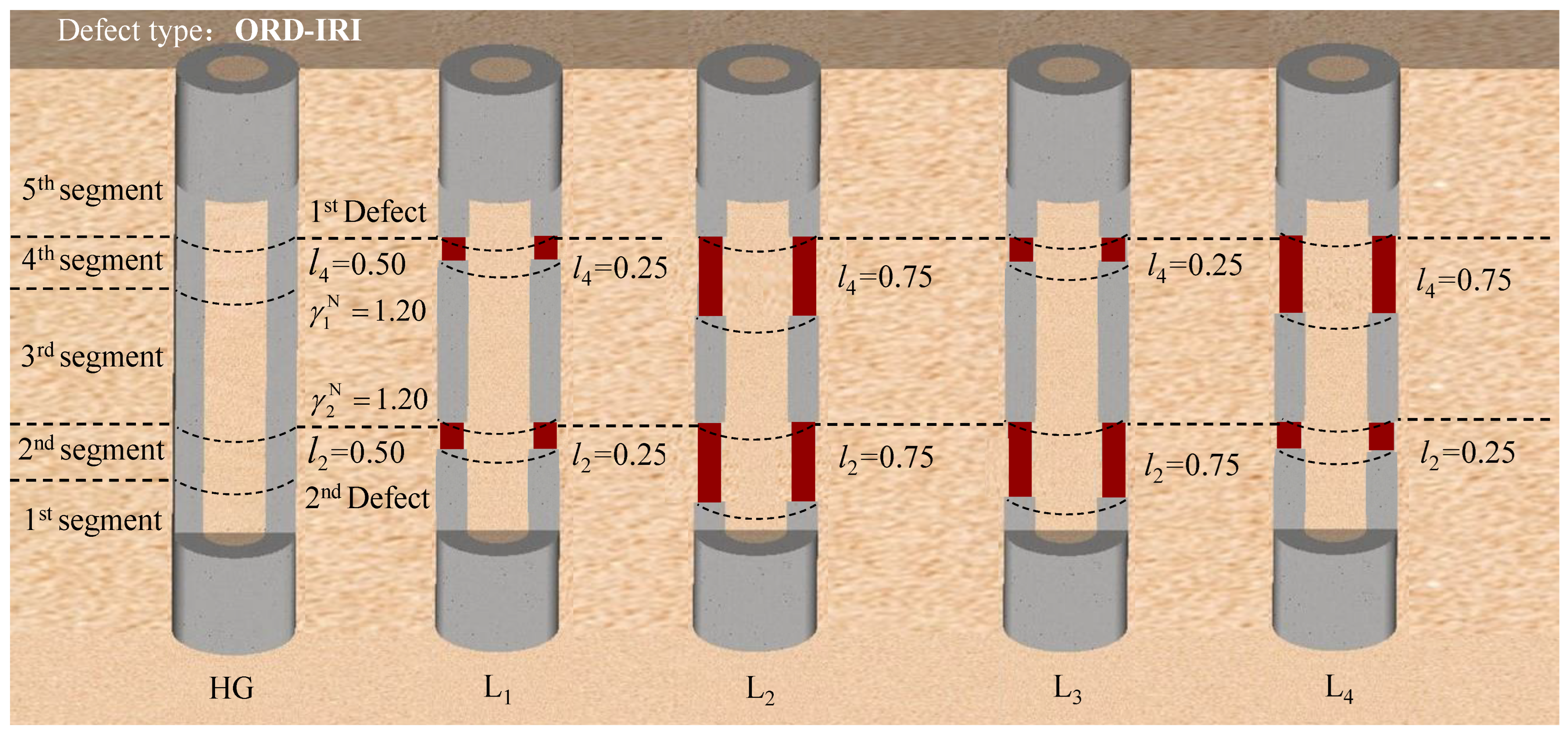
The amplitude difference between adjacent crests rises with the increase in the length of necking defects, and the closer the necking defect to the pile head, the greater the AD that is caused by the increase in the defect length. The necking defect length increase also leads to a decrease in the amplitude of the pile tip signal, and this amplitude decrease mainly relates to the total lengths of multi-defects.
(5)
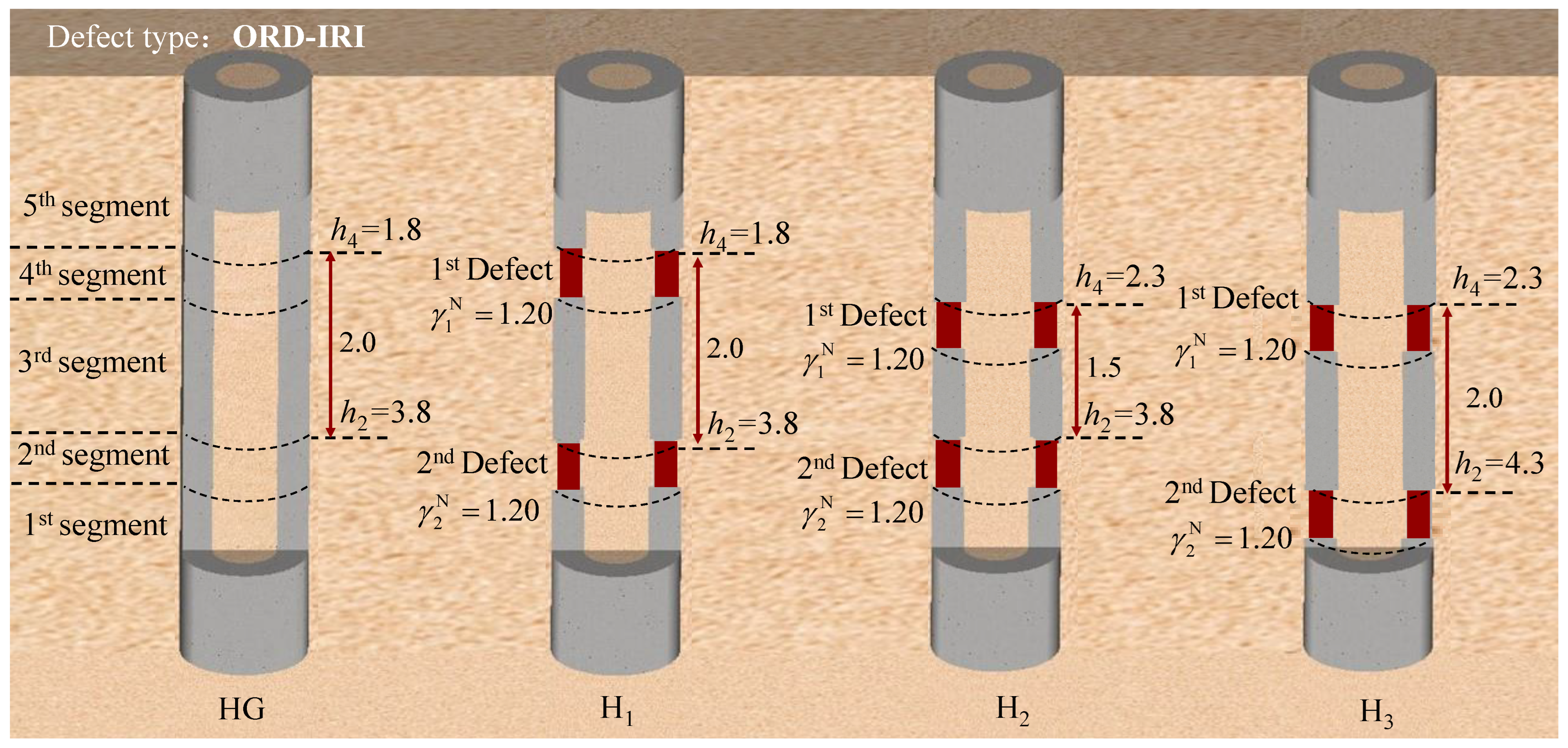
The deeper the depths of the defects, the greater the amplitude differences, and the closer the two defects, the smaller the amplitude differences. For the velocity response curve, the change in the defect depth leads to a time delay of the reflected signals from the relevant defect. In particular, the time difference between the reflected signals from the two defects is related to the distances of these defects.
The features of multi-defects appear to have different amplitude differences and reflected signal features on the velocity admittance and velocity response curves, respectively. This means that the obtained analytical solutions and relevant results can be used to detect multi-defects of pipe piles according to the different appearances of the velocity admittance and velocity response curve, as measured in engineering practice.

Author Contributions

Conceptualization, K.M.; methodology, K.M.; software, M.Z.; validation, M.Z.; formal analysis, M.Z.; investigation, M.Z.; resources, M.Z.; data curation, K.M.; writing—original draft preparation, K.M.; writing—review and editing, K.M.; visualization, M.Z.; supervision, K.M.; project administration, M.Z.; funding acquisition, K.M. All authors have read and agreed to the published version of the manuscript.

Funding

This research was funded by the National Science Foundation for Young Scientists of China, grant number 52108326.

Institutional Review Board Statement

Not applicable.

Informed Consent Statement

Not applicable.

Data Availability Statement

Not applicable.

Conflicts of Interest

The authors declare no conflict of interest.

References

  1. Yuan, B.; Li, Z.; Chen, W.; Zhao, J.; Lv, J.; Song, J.; Cao, X. Influence of Groundwater Depth on Pile–Soil Mechanical Properties and Fractal Characteristics under Cyclic Loading. Fractal Fract. 2022, 6, 198. [Google Scholar] [CrossRef]
  2. Ni, S.-H.; Yang, Y.-Z.; Tsai, P.-H.; Chou, W.-H. Evaluation of pile defects using complex continuous wavelet transform analysis. NDT E Int. 2017, 87, 50–59. [Google Scholar] [CrossRef]
  3. Chen, L.; Wu, W.; Liu, H.; El Naggar, M.H.; Wen, M.; Wang, K. Influence of defects on the lateral dynamic characteristics of offshore piles considering hydrodynamic pressure. Ocean Eng. 2022, 260, 111894. [Google Scholar] [CrossRef]
  4. Meng, K.; Su, H. Analytical model of large-diameter viscoelastic floating pile and application in pile low-strain integrity testing. Soil Dyn. Earthq. Eng. 2022, 158, 107296. [Google Scholar] [CrossRef]
  5. Zhang, Y.; El Naggar, M.H.; Wu, W.; Wang, Z. Torsional Low-Strain Test for Nondestructive Integrity Examination of Existing High-Pile Foundation. Sensors 2022, 22, 5330. [Google Scholar] [CrossRef]
  6. Anoyatis, G.; Mylonakis, G. Dynamic Winkler Modulus for Axially Loaded Piles. Geotechnique 2012, 62, 521–536. [Google Scholar] [CrossRef] [Green Version]
  7. Ye, Z.; Ai, Z.Y. Vertical Dynamic Response of a Pile Embedded in Layered Transversely Isotropic Unsaturated Soils. J. Geotech. Geoenviron. Eng. 2022, 148, 04021169. [Google Scholar] [CrossRef]
  8. Lü, S.; Wang, K.; Wu, W.; Leo, C.J. Longitudinal vibration of a pile embedded in layered soil considering the transverse inertia effect of pile. Comput. Geotech. 2014, 62, 90–99. [Google Scholar] [CrossRef]
  9. Liu, X.; El Naggar, M.H.; Wang, K.; Wu, J. Three-dimensional axisymmetric analysis of pile vertical vibration. J. Sound Vib. 2021, 494, 115881. [Google Scholar] [CrossRef]
  10. Michaelides, O.; Gazetas, G.; Bouckovalas, G.; Chrysikou, E. Approximate non-linear dynamic axial response of piles. Géotechnique 1998, 48, 33–53. [Google Scholar] [CrossRef]
  11. Yesilce, Y.; Catal, H.H. Free vibration of piles embedded in soil having different modulus of subgrade reaction. Appl. Math. Model. 2008, 32, 889–900. [Google Scholar] [CrossRef]
  12. Mylonakis, G. Winkler modulus for axially loaded piles. Géotechnique 2001, 51, 455–461. [Google Scholar] [CrossRef]
  13. Novak, M. Dynamic Stiffness and Damping of Piles. Can. Geotech. J. 1974, 11, 574–598. [Google Scholar] [CrossRef]
  14. Wu, W.; Wang, K.; Zhang, Z.; Leo, C.J. Soil-pile interaction in the pile vertical vibration considering true three-dimensional wave effect of soil. Int. J. Numer. Anal. Methods Géoméch. 2013, 37, 2860–2876. [Google Scholar] [CrossRef]
  15. Wang, K.; Wu, W.; Zhang, Z.; Leo, C.J. Vertical dynamic response of an inhomogeneous viscoelastic pile. Comput. Geotech. 2010, 37, 536–544. [Google Scholar] [CrossRef]
  16. Gao, L.; Wang, K.; Xiao, S.; Li, Z.; Wu, J. An analytical solution for excited pile vibrations with variable section impedance in the time domain and its engineering application. Comput. Geotech. 2016, 73, 170–178. [Google Scholar] [CrossRef]
  17. Wu, J.; Wang, K.; El Naggar, M. Dynamic response of a defect pile in layered soil subjected to longitudinal vibration in parallel seismic integrity testing. Soil Dyn. Earthq. Eng. 2019, 121, 168–178. [Google Scholar] [CrossRef]
  18. Wu, J.; Wang, K.; El Naggar, M.H. Dynamic soil reactions around pile-fictitious soil pile coupled model and its application in parallel seismic method. Comput. Geotech. 2019, 110, 44–56. [Google Scholar] [CrossRef]
  19. Zheng, H.; Ertel, J.-P.; Kourmpetis, M.; Kanfoud, J.; Niederleithinger, E.; Gan, T.-H. Integrity Testing of Cast In Situ Concrete Piles Based on an Impulse Response Function Method Using Sine-Sweep Excitation by a Shaker. J. Nondestruct. Eval. 2019, 38, 55. [Google Scholar] [CrossRef]
  20. Liu, X.; El Naggar, M.H.; Wang, K.; Wu, J. Vertical response analysis at multi-points on defective pile in layered soil and its application. Soil Dyn. Earthq. Eng. 2020, 139, 106358. [Google Scholar] [CrossRef]
  21. Wu, J.; Wang, K.; El Naggar, M.H. Half-space dynamic soil model excited by known longitudinal vibration of a defective pile. Comput. Geotech. 2019, 112, 403–412. [Google Scholar] [CrossRef]
  22. Yang, J.; Sun, X.-L.; Bian, D.-C.; Shao, J.-X. Large-scale model test for detecting pile defects using the parallel seismic method. Soil Dyn. Earthq. Eng. 2020, 139, 106300. [Google Scholar] [CrossRef]
  23. Basack, S.; Karami, M.; Karakouzian, M. Pile-soil interaction under cyclic lateral load in loose sand: Experimental and numerical evaluations. Soil Dyn. Earthq. Eng. 2022, 162, 107439. [Google Scholar] [CrossRef]
  24. Cao, X.; Wang, S.; Gong, W.; Wu, W.; Dai, G.; Zhou, F. Experimental and theoretical study on dynamic stiffness of floating single pile and pile groups in multi-layered soil. Soil Dyn. Earthq. Eng. 2022, 157, 107282. [Google Scholar] [CrossRef]
  25. Liu, H.-L.; Chu, J.; Deng, A. Use of large-diameter, cast–in situ concrete pipe piles for embankment over soft clay. Can. Geotech. J. 2009, 46, 915–927. [Google Scholar] [CrossRef] [Green Version]
  26. Li, Z.; Gao, Y. Effects of inner soil on the vertical dynamic response of a pipe pile embedded in inhomogeneous soil. J. Sound Vib. 2019, 439, 129–143. [Google Scholar] [CrossRef]
  27. Zheng, C.; Liu, H.; Ding, X.; Kouretzis, G. Resistance of inner soil to the vertical vibration of pipe piles. Soil Dyn. Earthq. Eng. 2017, 94, 83–87. [Google Scholar] [CrossRef]
  28. Zheng, C.; Hua, J.; Ding, X. Torsional vibration of a pipe pile in transversely isotropic saturated soil. Earthq. Eng. Eng. Vib. 2016, 15, 509–517. [Google Scholar] [CrossRef]
  29. Zheng, C.; Ding, X.; Sun, Y. Vertical Vibration of a Pipe Pile in Viscoelastic Soil Considering the Three-Dimensional Wave Effect of Soil. Int. J. Géoméch. 2016, 16, 04015037. [Google Scholar] [CrossRef]
  30. Liu, H.; Zheng, C.; Ding, X.; Qin, H. Vertical dynamic response of a pipe pile in saturated soil layer. Comput. Geotech. 2014, 61, 57–66. [Google Scholar] [CrossRef]
  31. Ding, X.; Liu, H.; Kong, G.; Zheng, C. Time-domain analysis of velocity waves in a pipe pile due to a transient point load. Comput. Geotech. 2014, 58, 101–116. [Google Scholar] [CrossRef]
  32. Li, Z.; Wang, K.; Wu, W.; Leo, C.J.; Wang, N. Vertical vibration of a large-diameter pipe pile considering the radial inhomogeneity of soil caused by the construction disturbance effect. Comput. Geotech. 2017, 85, 90–102. [Google Scholar] [CrossRef]
  33. Zheng, C.; Liu, H.; Kouretzis, G.P.; Sloan, S.W.; Ding, X. Vertical response of a thin-walled pipe pile embedded in viscoelastic soil to a transient point load with application to low-strain integrity testing. Comput. Geotech. 2015, 70, 50–59. [Google Scholar] [CrossRef]
  34. Zhou, M.; Liu, H.; Hossain, M.S.; Hu, Y.; Zhang, T. Numerical simulation of plug formation during casing installation of cast-in-place concrete pipe (PCC) piles. Can. Geotech. J. 2016, 53, 1093–1109. [Google Scholar] [CrossRef] [Green Version]
  35. Lysmer, J.; Richart, F.E. Dynamic Response of Footings to Vertical Loading. J. Soil Mech. Found. Div. 1966, 92, 65–91. [Google Scholar] [CrossRef]
  36. Wang, K.H.; Yang, D.Y.; Zhang, Z.Q.; Leo, C.J. A new approach for vertical impedance in radially inhomogeneous soil layer. Int. J. Numer. Anal. Methods Géoméch. 2011, 36, 697–707. [Google Scholar] [CrossRef]
Figure 1. Simplified mechanical model.
Jmse 11 00083 g001
Figure 2. Comparisons of the proposed solution with the solution of Wang et al. [36]. (a) K r , (b) K i .
Jmse 11 00083 g002
Figure 3. Different necking types of pipe piles.
Jmse 11 00083 g003
Figure 4. Effect of pile necking on the response of pile. (a) H v , (b) V v .
Jmse 11 00083 g004
Figure 5. Diagram of necking degree.
Jmse 11 00083 g005
Figure 6. Effect of necking degree on the pipe pile response. (a) H v , (b) V v .
Jmse 11 00083 g006
Figure 7. Diagram of defect distribution.
Jmse 11 00083 g007
Figure 8. Effect of defect distribution on the pipe pile response. (a) H v , (b) V v .
Jmse 11 00083 g008
Figure 9. Diagram of necking defect with different lengths.
Jmse 11 00083 g009
Figure 10. Effect of the length of necking defects on the pipe pile response. (a) H v , (b) V v .
Jmse 11 00083 g010
Figure 11. Diagram of necking defect with different depths.
Jmse 11 00083 g011
Figure 12. Effect of the depth of necking defects on the pipe pile response. (a) H v , (b) V v .
Jmse 11 00083 g012
Table 1. The parameters for numerical instances.
H = 6 m E k P = 25 GPa δ p = 100 kN / m 3 ρ k 1 = ρ k 0 = 2000 kg / m 3 G k 0 = G k 1 = 5 × 10 6 Pa
r k 0 = 0.30   m r k 1 = 0.60   m k p = 1000 kN / m 3 ρ k P = 2500 kg / m 3 η k 0 = η k 1 = 10 kN · s / m 2
Table 2. Length and depth of each pile segment.
n12345
lk (m)1.700.501.500.501.80
hk (m)4.303.802.301.800.00
Disclaimer/Publisher’s Note: The statements, opinions and data contained in all publications are solely those of the individual author(s) and contributor(s) and not of MDPI and/or the editor(s). MDPI and/or the editor(s) disclaim responsibility for any injury to people or property resulting from any ideas, methods, instructions or products referred to in the content.

