A Marine Hydrographic Station Networks Intrusion Detection Method Based on LCVAE and CNN-BiLSTM

Abstract

Marine sensors are highly vulnerable to illegal access network attacks. Moreover, the nation’s meteorological and hydrological information is at ever-increasing risk, which calls for a prompt and in depth analysis of the network behavior and traffic to detect network attacks. Network attacks are becoming more diverse, with a large number of rare and even unknown types of attacks appearing. This results in traditional-machine-learning (ML)-based network intrusion detection (NID) methods performing weakly due to the lack of training samples. This paper proposes an NID method combining the log-cosh conditional variational autoencoder (LCVAE) with convolutional the bi-directional long short-term memory neural network (LCVAE-CBiLSTM) based on deep learning (DL). It can generate virtual samples with specific labels and extract more significant attack features from the monitored traffic data. A reconstructed loss term based on the log-cosh model is introduced into the conditional autoencoder. From it, the virtual samples are able to inherit the discrete attack data and enhance the potential features of the imbalance attack type. Then, a hybrid feature extraction model is proposed by combining the CNN and BiLSTM to tackle the attack’s spatial and temporal features. The following experiments evaluated the proposed method’s performance on the NSL-KDD dataset. The results demonstrated that the LCVAE-CBiLSTM obtained better results than state-of-the-art works, where the accuracy, F1-score, recall, and FAR were 87.30%, 87.89%, 80.89%, and 4.36%. The LCVAE-CBiLSTM effectively improves the detection rate of a few classes of samples and enhances the NID performance.

1. Introduction

Regional marine hydrographic information (RMHI) includes sea temperature, ocean current conditions, and tidal cycles and their intensity, which are intimately related to the navigation conditions for vessels [1]. Therefore, RMHI is regarded as vital strategic information by various countries worldwide. In general, RMHI is usually monitored for normalization by permanent or semi-permanent automatic hydrographic monitoring stations (AHMSs) [2]. Only based on publicly available data, the U.S. National Oceanic and Atmospheric Administration (NOAA) has deployed more than 20,000 AHMSs in the global ocean as of 2022. Meanwhile, other countries are also accelerating the deployment of AHMSs with different specifications [3].

With the rapid development of 5G technology and IoT technology in recent years, automation and networking have become the most-common working mode of AHMSs [4,5]. Ordinarily, in a sea area, several adjacent AHMSs can be formed into a monitoring network [6]. In this network, the stations communicate with each other through wireless protocols, complete the initial data analysis, and package the data to upload to the cloud. This operation mode helps improve the robustness of RMHI, reduce the load on the network, and control the cost of data storage and downloading [3].

It is difficult to maintain hydrological monitoring networks (HMNs) deployed in remote oceans. The cloud computing strategy plays an important role in HMNs [7]. According to cloud computing, remote servers are able to store, read, and analyze the data. Because of this, highly automated HMNs are vulnerable to various forms of nefarious attacks (including man-in-the-middle attacks, network sniffing, denial-of-service attacks, port scanning, and other forms of attack) [8]. Once the HMN is under these attacks, confidential RMHI may be leaked, threatening national strategic security. In this context, an intrusion detection system (IDS), which enables detecting and alerting about network intrusions by identifying network traffic data (NTD), is essential in the HMN.

In terms of detection devices, host-based IDSs (HIDSs) and network-based IDSs (NIDSs) are the most-popular types of network intrusion detection (NID) systems [9]. The former are mainly deployed in local devices (e.g., PCs, database devices, etc.) and detect network intrusions by analyzing the operation behavior of the files [10]. NIDSs are generally used to prevent network attacks against the server layer. There are two typical operation strategies for NIDSs, signature and anomaly [11]. The former defines a set of rules to determine whether a network behavior is an intrusion based on the description from known attack behavior features. This approach performs well for known attacks, but weakly detects unprecedented attacks (0-day attacks). Anomaly NIDSs analyze a large amount of normal NTDSs to obtain the best features of the normal network behavior. They are not sensitive to the attack occurrence frequency, obtain better generalization ability, and have gained wide attention in recent years.

NIDs can be regarded as a classification problem with respect to network behavior. In the past two decades, much research has been carried out in this area to propose a more advanced intrusion detection method [12,13]. Some Euclidean-distance-based ML methods were first applied to this field, such as k-nearest neighbors (KNNs), support vector machine (SVM), and logistic regression (LR) [8,14,15]. These methods may have satisfactory performance in a simple network environment, but because they cannot effectively trace the deeper features of the intrusion behavior, they are not suited to handling today’s diverse attacks [16].

Since the 2010s, DL technology has developed significantly, and the GAN, SAE, DNN, and other related algorithms are widely used in NIDs [17,18]. DL-based detection methods are adept at extracting abstract features from massive amounts of NTDs. They overcome the limitations of shallow ML algorithms and provide a new way of more accurate intrusion detection. However, for AHMSs, these methods generally suffer from the following two drawbacks:

(1) DL cannot address unbalanced intrusion samples. The actual NTD database often contains a large number of normal behaviors and a small number of attacks. At the same time, even with this minority of attacks, it may be filled with a number of 0-day attacks. This is fatal for DL methods that heavily rely on large amounts of data for training. They may not be able to obtain enough effective features in the training phase, especially for those 0-day attacks [19]. AHMSs typically work in a unattended and open environment. They are exposed to more diverse security threats, and AHMSs are vulnerable to new types of cyber attacks at all times. Therefore, the effectiveness of traditional DL-based detection methods is a concern for AHMSs.

(2) DL fails to consider the time cost of intrusion detection [20]. Since the actual NTD generally has high-dimensional characteristics (above 40 dimensions), complex detection neural networks incur a huge computational load, which takes much time and even affects the real-time performance of detection. On the other hand, due to cost considerations, AHMSs generally do not have high-performance master control units. Therefore, they are extremely inefficient in handling complex intrusion detection algorithms. We are very clear that too delayed detection results are meaningless, and the damage caused by the attack may have been irreversible.

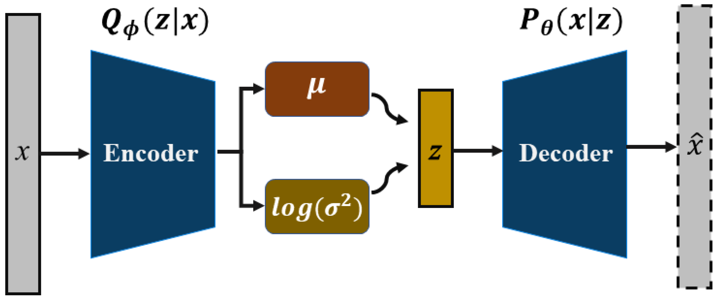
In order to solve the dilemma faced by AHMSs and secure RMHI transmission and storage, this paper proposes a BiLSTM combining the CNN NID method based on the LCVAE. As show in Figure 1 , the overall structure of the LCVAE-CBiLSTM, which consists of two main parts, the encoder and the classification. The former can be regarded as an extended model of the VAE and CVAE. A basic VAE consists of an encoder and a decoder to model the distribution of observed data by latent variables in an unsupervised manner [21]. On this basis, the CVAE can refer to the sample feature vector by itself to guide the encoder generation process and obtain more efficient features in the potential space [22]. More importantly, it can generate new samples given conditional information (labels). In the classification part, the CNN is used to extract the data features in space. Considering the NTD’s potential sequential features, BiLSTM can extract its temporal features further. Moreover, this model will reduce the data dimension and control the detection time [23,24].

In summary, the main contributions of this paper are as follows:

(1) We introduced the CVAE to the NID for reconstructing attack samples in the NTD. On the basis of the CVAE, we constructed the loss function using the log-cosh function. This enables the novel LCVAE to better extract the discrete features of the NTD. It also allows the new samples generated by the LCVAE to complement the minority types and provide a database for more accurate intrusion detection.

(2) We constructed a classification model combining the CNN and BiLSTM. Among them, the CNN is suitable for extracting local spatial features and BiLSTM takes into account bi-directional time series information. The model can analyze the NTD in two dimensions, time and space, to extract more significant network behavior features, which provides a guarantee for a more accurate NID. The multiple-feature extraction strategy also effectively controls the data’s dimensionality to ensure the intrusion detection’s efficiency.

(3) We evaluated the accuracy of the LCVAE-CBiLSTM compared to several other state-of-the-art works in a simulation environment. A miniature hydrological monitor was developed to evaluate the efficiency of different methods on a low-power platform. The experimental results show that our model is superior to other methods in detection performance. This demonstrates that the LCVAE-CBiLSTM provides an effective method for intrusion detection.

The remaining parts of this article are organized as follows. Section 2 introduces the related works. Section 3 describes the proposed algorithm’s theory in detail. Section 4 shows the experimental setup, experimental results, and discussion. Section 5 provides the conclusion of the work, as well as future work.

2. Related Works

Machine learning strategies have been long applied to improve IDS through hybrid models. Zhao proposed a method based on the hybrid kernel function least-squares support vector machine (LSSVM) [25]. He introduced a particle swarm optimization (PSO) algorithm to find the optimal parameters in the LSSVM, which effectively improved the accuracy of intrusion detection. Tao used a genetic algorithm (GA) to select features, weights, and parameters in SVM [26]. Compared to the traditional SVM approach, his strategy had better performance in terms of the accuracy rate and the false alarm rate. In order to improve the detection efficiency, Peng filtered the more significant traffic features with the network behavior by principal component analysis (PCA) first and, then, identified the attack type by K-means [27].

Traditional ML methods all belong to shallow learning. Along with the development of the Internet, the large number of more complex and hidden nonlinear network features brings new challenges to NID. DL algorithms are able to extract high-level abstract features from the original samples through multiple iterations. Therefore, they will effectively overcome the limitations of ML methods and improve detection accuracy. The use of DL methods for NID has become a trend in recent years [28].

Some neural-network-based classification models have been proposed. Ingre deployed artificial neural networks (ANNs) for IDSs, but the experimental results on a publicly available network traffic dataset, NSL-KDD, did not show model superiority [29]. He also tried to propose several hybrid detection methods combining different algorithms, but the results still needed improvement. Yan proposed a greedy multilayer deep belief network model (GDBN) [30]. The model focuses on using the restricted Boltzmann machine (RBM) to separate noisy and anomalous data in the samples [31]. A back-propagation strategy was used to control the training parameters in the DBN, which in turn implemented the NID. Tang selected six basic features from the NSL-KDD dataset using the software-defined networking (SDN) strategy [32]. These features support effective network behavior classification by a simple deep neural network (DNN). The above DL-based NID approaches ignore the imbalance of samples in NID, which has resulted in no significant improvement in the detection performance for IDS for a long time.

At present, there are two main types of solutions for the imbalanced characteristics of the samples: algorithmic compensation and data compensation. The former considers the model’s sensitivity to different intrusion types and improves the detection accuracy by designing the attack detection weights [33]. However, since the weights of 0-day attacks are unknown, the algorithmic compensation method is constantly weak when dealing with them [34]. Data compensation reduces the degree of type imbalance in modifying the original sample distribution. Simply put, it adds minority-type samples or removes a part of the normal samples. Common methods are the random oversampler (ROS) [35], synthetic minority oversampling technique (SMOTE) [36], variational autoencoder (VAE) [37], etc. DL can extract additional significant intrusion features from minority types that have already been increased. Numerous experiments have shown that combining data compensation and DL is a unique NID method. This means that this hybrid technique has much promise for study in intrusion detection.

The VAE is a feature extraction algorithm derived from the autoencoder (AE) [37,38]. The AE uses a neural network to fit a mapping relationship from sample $\mathit{x}$ to a potentially encoded sample $\mathit{z}$. For a high-dimensional $\mathit{x}$, the structure of $\mathit{z}$ may be straightforward. Since the mapping relationship between $\mathit{x}$ and $\mathrm{z}$ is unique, the AE does not work for data generation. In NID, the AE is more often used for feature dimensionality reduction. The VAE assumes $x\to z$ tallies with a normal distribution. After describing the encoding process of $\mathit{z}$ by means and variances, the new data can be obtained by sampling from them. However, the VAE uses an unsupervised learning strategy, and we cannot control the generated data by the distribution of the samples. There is not much one VAE can do to solve the problem of attack imbalance. To address the problem, Kingma proposed the conditional variational autoencoder (CVAE) [22]. It establishes a distribution relationship between sample labels $\mathit{c}$ and $\mathit{z}$ based on the VAE. In other words, the class of $\mathit{z}$ can be determined by $\mathit{c}$. This feature makes the decoder of the CVAE generate the specified data type. It is of great significance for NID because it enables expanding minority attacks in the original sample and helps the intrusion detection algorithm dig out deeper features.

The CVAE-based NID model designed by Martin is poor in intrusion detection, but he validated that the data generation capability of the CVAE can be used in IDS [39]. Hannan was not interested in data generation. He focused on a semi-supervised CVAE-based feature extraction method by marking attack data in the training set [40]. The experimental results showed that the CVAE was more satisfactory for the detection on the CIC-IDS2017 dataset than other traditional methods, but less effective for NSL-KDD. Liu compared the detection effectiveness of the VAE and CVAE for NTDs in the setting of the CNN and RNN as the classifiers [41]. In the experiments for the CSE-CIC-IDS2018 dataset, he found that the CVAE can effectively improve the detection of NIDs from multiple scales such as the precision, recall, and F1-score. However, some scholars have pointed out some drawbacks of the CVAE deployed on NID. (1) The CVAE suffers from KL vanishing in training, which leads to the model’s failure to converge [42]. (2) The L2 loss function in the traditional CVAE tends to result in local optima and is sensitive to noise [43]. In this context, many CVAE-based improvement models have been proposed. For example, the supervised adversarial variational autoencoder with regularization (SAVAER), the classwise focal loss variational autoencoder (CFLVAE), the conditional denoising adversarial autoencoder (CDAAE), etc., but these methods failed to bring better performance to NID [43,44,45].

Recently, related scholars have attempted to combine multiple DL methods into a hybrid model to improve intrusion detection performance. Hawawreh proposed an NID model combining a deep autoencoder with a deep feed-forward neural network (DAE-DFFNN), which validated the possibility of hybrid models [46]. Zhang proposed the CWGAN-CSSAE, which combines the improved conditional Wasserstein generative adversarial network and cost-sensitive stacked autoencoders. The experimental results on the KDDTest-21 showed that the detection accuracy was improved by 2–5% compared to other simple DL models [47].

Combining the advantages of the above methods, this paper first proposes an LCVAE model, which avoids the problem of KL divergence for insufficient control of the model by introducing a log-cosh function to reconstruct the loss term of the CVAE. Then, we expand the original dataset with the few classes of attack samples generated by the LCVAE to provide sufficient training conditions for the classifier. Finally, a hybrid detection model, the CNN-BiLSTM, is constructed to ensure intrusion detection accuracy.

3. Methods

The flowchart of the proposed LCVAE-CBiLSTM method is shown in Figure 2 and consists of 4 steps:

Step 1: numerical processing. To make the intrusion detection model more accurate in identifying the data features, at the beginning of all processes, performing the necessary pre-processing of the original data is necessary. It first digitizes the character-based features and, then, normalizes each feature. Then, it separates the training set and testing set from the dataset.

Step 2: LCVAE-based sample generator for minority class attacks. DL-based detection algorithms are usually insensitive to a few classes of samples. We propose an improved CVAE algorithm for generating minority class attack samples to enforce their missing features. The training set data are fed into the model to obtain the newly generated enhanced data.

Step 3: Hybrid feature extraction strategy. In order to comprehensively extract features from traffic data that are more closely associated with attack behavior, we designed a hybrid feature extraction strategy. In this strategy, the CNN is used to extract the spatial features of the samples, and the BiLSTM is used to extract the temporal features. The training set and the enhanced data are fed into the proposed algorithm after the iterations of training to obtain a high-performance feature extraction model.

Step 4: Obtain test results. We input the testing set into the model obtained by Step 3 to extract the deep features of the samples. Finally, a Softmax algorithm completes the intrusion decision based on these features.

3.1. Data Preprocessing

Data preprocessing includes two steps as follows:

Numerical processing.

The three symbolic features (protocol_type, service protocol, and flag protocol) in NSL-KDD need to be converted into digital features to facilitate model training. We used one-hot encoding to accomplish this task. The above three features are converted into 3, 70, and 11 numeric features. Together with the original 38 numeric features, the original 41-dimensional features become 122-dimensional after numerical processing. It is worth noting that the feature $\mathit{num}$_$outbound$_$cmds$ is all 0, which can be considered a redundant feature [29]. Therefore, we removed it and finally obtained 121-dimensional features.

Normalization processing.

In NTDs, the difference in the range of values of various features may be too huge. For example, in NSL-KDD, the $\mathit{num}$_$root$ feature takes a range of [0,7468], while the $\mathit{num}$_$shells$ feature only takes a range of [0, 5]. In DL, the exaggerated range of feature values would lead to the model not being able to converge. Therefore, we completed the normalization process for all the features by mapping each feature within the [0, 1] interval uniformly and linearly. The normalization process for variable X is shown in Equation (1).

$$X_{\mathrm{nom}}=\frac{X-X_{min}}{X_{max}-X_{min}}$$

(1)

In Equation (1), $X_{max}$ is the maximum value of the sample data, $X_{min}$ is the minimum value of the sample data, and $X_{\mathrm{nom}}$ is the data after normalization.

3.2. Log-Cosh Conditional Variational Autoencoder

The VAE and CVAE are the prerequisites for understanding the mechanism of the LCVAE. Assume that the original sample is $\mathit{x}$ and the generated sample by the model is $\widehat{x}$. A typical CVAE model is shown in Figure 3, which adds a conditional factor $\mathrm{c}$ (which can be interpreted as the sample’s label) to the VAE. The target of the encoder $Q_{\varphi }$ in the VAE is to establish a mapping relationship from the original high-dimensional sample $\mathit{x}$ to the low-dimensional feature vector $\mathrm{z}$ through a neural network. In Figure 3, the CVAE introduces $\mathit{c}$ as a selection condition for $\mathit{x}$, at which point, the mapping relationship from $\mathit{x}$ to $\mathit{z}$ is $\mathit{z}\sim Q_{\varphi }(\mathit{z}\mid \mathit{x},\mathit{c})$. In contrast, the decoder $P_{\theta }$ constructs a neural network $\widehat{x}\sim P_{\theta }(\mathit{x}\mid \mathit{z},c)$ that maps $\mathit{z}$ and $\mathit{c}$ back to $\widehat{x}$. The objective loss function of the VAE is shown in Equation (2).

$$\begin{array}{cc}\hfill L_{VAE}=& {\mathbb{E}}_{Q(z\mid x)}[logp\left(x\right)]\hfill \\ \hfill & =\underset{\mathrm{Reconstruct}\mathrm{term}{L}_{\mathrm{Rec}}}{\underbrace{{\mathbb{E}}_{Q(z\mid x)}[logP(x\mid z)]}}-\underset{KL\mathrm{term}{L}_{KI}}{\underbrace{D_{KL}(Q(z\mid x)\parallel P\left(z\right))}}\hfill \end{array}$$

(2)

Then, the CVAE loss function model can be introduced as:

$$\begin{array}{cc}\hfill L_{CVAE}=& {\mathbb{E}}_{Q(z\parallel x)}[logP(x\mid c)]\hfill \\ \hfill & =\underset{\mathrm{Reconstruct}\mathrm{term}{L}_{\mathrm{Rec}}}{\underbrace{{\mathbb{E}}_{Q(z\parallel x,c)}[logP(x\mid z,c)]}}-\underset{KL\mathrm{term}{L}_{KI}}{\underbrace{D_{KL}(Q(z\mid x,c)\parallel P(z\mid x,c))}}\hfill \end{array}$$

(3)

where the loss function consists of two components. (1) The first term, ${\mathbb{E}}_{Q(z\mid x,c)}[logP(x\mid z,c)]$, is a logarithmic reconstruction likelihood function that describes the correct rate of compressing high-dimensional features into a low-dimensional space and, then, restoring them correctly. (2) The second term, $D_{KL}(Q(z\mid x,c)\parallel P(z,c))$, evaluates the performance of the encoder and decoder by constructing the KL scatter of the prior and posterior distributions of $\mathit{z}$. Obviously, the training process of the CVAE is to ensure the maximization of the reconstruction term and the minimization of the KL scatter term in Equation (3). Due to the presence of the reconstruction term $P(x\mid z,c)$, the type of new samples generated can be selected by controlling $\mathit{z}$ and $\mathit{c}$.

From Equation (3), the reconstruction term is constructed based on the $L_2$ function, as shown in Equation (4).

$$L_{Rec}(x,\widehat{x})={\parallel x-\widehat{x}\parallel }_2^2=\sum _i{\left|x_i-\widehat{x}\right|}^2$$

(4)

In Equation (4), $x_i$ denotes the $\mathit{i}$th feature in $\mathit{x}$. Two shortcomings of $L_2$ limit the performance of the reconstructed model. $L_2$ will generate a large loss value when $\mathit{x}$ is significantly higher than $\widehat{x}$. It may cause a gradient explosion, and the reconstructed model may not converge effectively. Furthermore, the gradient explosion will seriously increase the time complexity and lead to a huge computational overhead of the model. Because of the presence of the squared term in $L_2$, when the loss value is small (<1), $L_2$ may ignore part of this error. It would cause the reconstruction model of the CVAE to be completely controlled by KL and even fall into the local optimum. Chen argued that this reconstruction model significantly weakens the accuracy of sample generation when dealing with high-dimensional features [48].

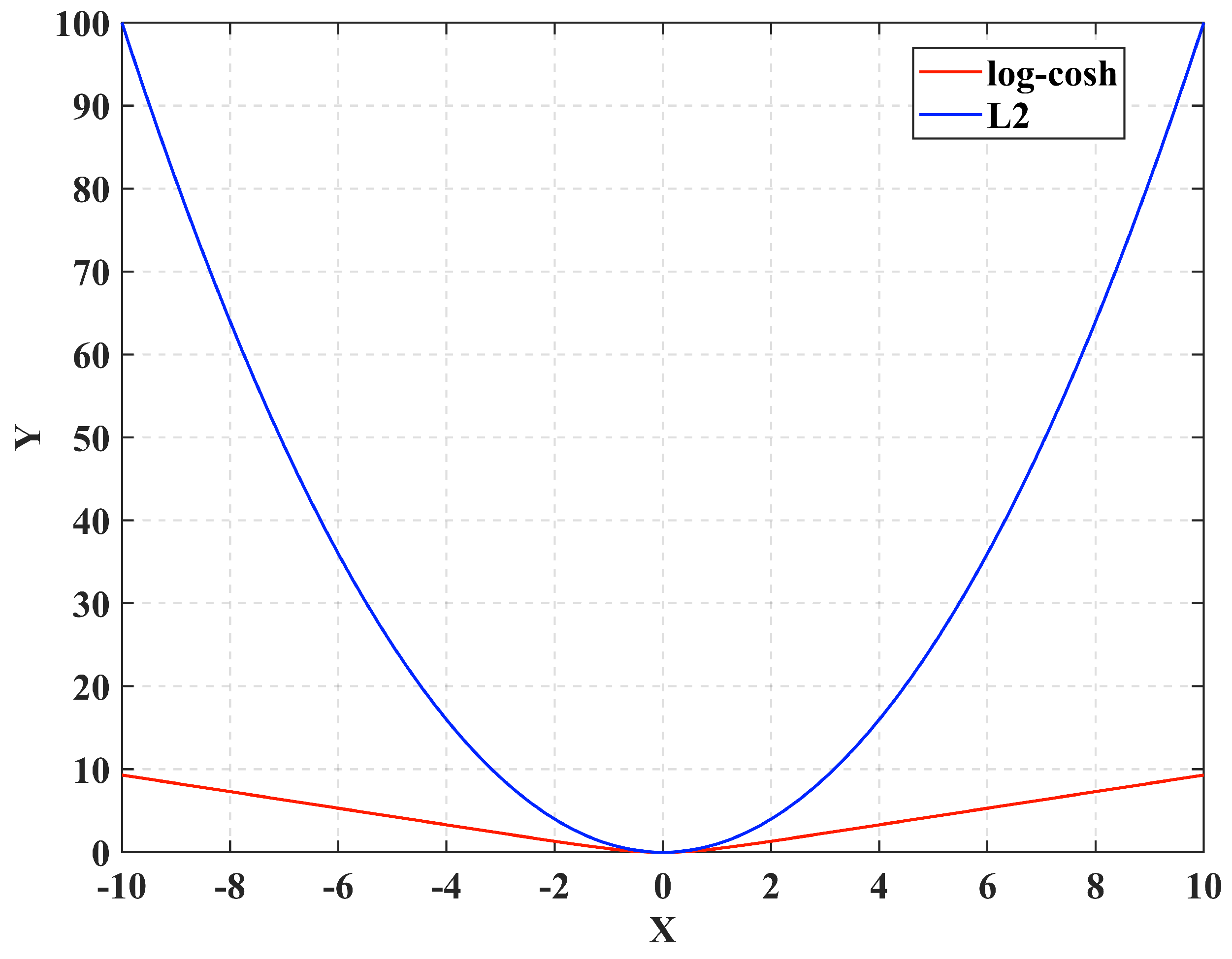
To solve the problem that the $L_2$ limits the performance of the CVAE, we propose the log-cosh function as the loss term of the reconstruction, as Equation (5):

$$L_{log-cosh}(x,\widehat{x})=\frac{1}{a}\sum _{i}log\left(cosh\left(a\left(x_i-{\widehat{x}}_i\right)\right)\right)$$

(5)

Equation (5) in $a\in R$ is a parameter. The images of log-cosh and $L_2$ are shown in Figure 4. It can be seen that, when the difference between $\mathrm{x}$ and $\widehat{x}$ is large, the loss value of the log-cosh is much smaller than $L_2$, which can effectively avoid the gradient explosion. On the contrary, when the loss is close to 0, the log-cosh gradient decreases, ensuring the model’s accuracy.

When the log-cosh replaces the reconstructed loss term of the CVAE, the proposed LCVAE model is shown by Equation (6).

$$L_{\mathrm{LCVAE}}=\frac{1}{a}\sum _{i}log\left(cosh\left(a\left(x_i-{\widehat{x}}_i\right)\right)\right)-D_{KI}(Q(z\mid x,c)\parallel P(z\mid x,c))$$

(6)

The percentage of certain attack types might be quite low because there is an imbalance in the types of network traffic. For example, samples belonging to the remote-to-local and user-to-root account for less than 1% of the KSL-KDD dataset. Most intrusion detection algorithms are powerless to deal with similar minority classes. Even though they are non-converging when training the detection model, the meager ratio cannot affect the model’s overall training results. This will cause the detection models to ignore the detection sensitivity of these types.

Similar to the traditional CVAE, in the LCVAE, Equation (6) is used as the loss function to train the generator. We first chose $\mathit{c}$ as belonging to the minority types in the dataset generation phase. The appropriate $\mathit{z}$ is determined by the normal distribution of $\mathit{c}$ and fed back to the decoder network to generate new intrusion samples. By adding the generated $\widehat{x}$ to the original dataset, the minority types sample in the whole dataset may be increased to alleviate the data category imbalance.

3.3. Temporal Features Extraction by BiLSTM

Considering the potential temporal correlation of NTD, a neural network model combining the BiLSTM [19], as shown in Figure 5, was established to extract the temporal features.

As can be seen from Figure 5, the BiLSTM is formed by two inverse LSTM networks. The single LSTM network consists of multiple neuron nodes. Each neuron node contains three decision-makers: the input gate, the output gate, and the forget gate. The computational flow of each neuron node in the LSTM is as follows.

The state $h_{t-1}$ of the hidden layer at the moment $t-1$ and the input $x_t$ at moment t are fed into the forget gate of a new neuron node. Equation (7) determines whether the information of the current input $x_t$ will be updated in the neuron, where W is the weight matrix and b is the decision preference.

$$i_t=\sigma \left(W_t·\left[h_{t-1},x_t\right]+b_t\right)$$

(7)

At this point, the input gate also generates ${\tilde{C}}_t$ to describe the temporary state of the neuron node, as shown in Equation (8).

$${\tilde{C}}_t=tanh\left(W_C·\left[h_{t-1},x_t\right]+b_C\right)$$

(8)

Then, the input gate will determine the information that the neuron node at moment t will retain from $h_{t-1}$ based on $x_t$, as shown in Equation (9).

$$f_t=\sigma \left(W_f·\left[h_{t-1},x_t\right]+b_f\right)$$

(9)

The forget gate selects the information that needs to be updated from the node’s state at $t-1$. The input gate will control the temporary state that needs to be retained. The current node state C will be obtained by associating the node states of these two temporal states:

$$C_t=f_t*C_{t-1}+i_t*{\tilde{C}}_t$$

(10)

Finally, the output gate will update the state of the hidden layer, as shown in Equation (11).

$$h_t=\sigma \left(W_o\left[h_{t-1},x_t\right]+b_o\right)*tanh\left(C_t\right)$$

(11)

In Figure 5, two LSTM networks are responsible for the forward and backward feature extraction, respectively. Using the BiLSTM model provides a better consideration of the effect of each attribute before and after in the sequence data and obtains more comprehensive feature information. The BiLSTM states at time t include the forward and backward outputs, as shown in Equations (12)–(14).

$$h_t^{\mathrm{forward}}=LST{M}^{\mathrm{forward}}\left(h_{t-1},x_t,C_{t-1}\right)$$

(12)

$$h_t^{\mathrm{backward}}=LST{M}^{\mathrm{backward}}\left(h_{t-1},x_t,C_{t-1}\right)$$

(13)

$$H_t=\left[h_t^{\mathrm{forward}},h_t^{\mathrm{backward}}\right]$$

(14)

3.4. Convolutional Neural Network

Besides temporal features, the huge amount of NTD data also has significant spatial features. Therefore, we designed a CNN model before the BiLSTM to extract the spatial distribution features. Furthermore, the multi-layer convolution and pooling process enables the downsizing of the features and improves the computational efficiency of the BiLSTM network.

In the CNN, the NTDs are firstly spread into a matrix of size n*m after pre-processing. This matrix is input into the convolution layer, and the convolution process is shown in Equation (15).

$$Z=f(M\otimes W+b)$$

(15)

where M is the feature map. b is the bias. ⊗ is the convolution function, and $f\left(x\right)$ is the activation function. $f\left(x\right)$ helps to reduce the linearity of the model and improve the performance of model feature extraction.

It is important to create a nonlinear mapping for each convolutional kernel’s convolution result in order to facilitate the computation. Here, we used the RULE activation function, as show in Equation (16).

$$f\left(x\right)=RULE=max(0,x)$$

(16)

Then, the activated feature vectors are integrated by a pooling layer. The maximum value is kept in a window of a certain size to reduce the size of the output features and avoid transition fitting.

After several convolutional and pooling processes, the output of the CNN is reshaped into a one-dimensional vector by one fully connected layer. This one-dimensional vector is the one that contains the spatial features of the NTD.

3.5. CNN-BiLSTM Feature Extraction Model

After introducing the CNN, the CNN-BiLSTM network model as shown in Figure 6 is established to extract the NTD’s features.

By combining the CNN and BiLSTM, the layered network model is established to extract the spatiotemporal features of the NTD simultaneously, in which the CNN uses two sets of convolutional–pooling layers to complete the extraction of the spatial features. The strides of Conv1 and Conv2 are 1 and 3, respectively. In these two convolutions, the convolutional kernel size is 3*3, padding is 1, the activation function is tanh, the pooling kernel size is 2*2, and the pooling step is 2. A two-layer BiLSTM model was used for temporal feature extraction. The first BiLSTM contains 128 neurons, and the second contains 256. Each recursive operation of the BiLSTM results in the fusion of all previous and current features. A fully connected layer is linked to all output layers of the BiLSTM to combine the previously extracted features. Then, the fully connected layer’s output value is transmitted to a Softmax classifier to complete the network behavior detection. Finally, according to the extracted features, the network behavior is decided by a Softmax.

4. Experimental Validation and Analyses

This research conducted experiments on a desktop platform to evaluate the effectiveness of the proposed method. The detailed configuration of the platform is shown in

Table 1. Experimental platform.

Project	Configuration
Operation system	Windows 11
CPU	AMD-5700X 4.7–5.0 Ghz
GPU	NVIDIA 3060TI 8 G
Memory	32 G
Frame	Pytorch

. The experimental target dataset was NSL-KDD.

4.1. The Benchmark Datasets

The NSL-KDD dataset is an improved version of the KDDcup99 dataset [49]. It eliminates a large amount of duplicated and redundant data in KDDcup99, improves the sample quality, and has become a widely used intrusion detection dataset in recent years. NSL-KDD records 148,517 NTDs as samples, each sample consisting of 41 features and containing two subsets: (1) KDDTrain+ as a training set containing 125,973 samples, recording 22 types of attacks, and (2) KDDTest+ as a testing set containing 22,544 samples and 17 more types of attacks than KDDTrain+ to serve as 0-day attacks.

Table 2. Attack type distributions of NSL-KDD.

Category		Description	Data
			Train	Test
Attack	DoS	Malicious occupation of network resources.	45,927	7458
	Probe	Illegal obtaining users’ privacy.	11,656	24,218
	R2L	Hijack from a remote computer.	99	2754
	U2R	Illegal obtaining of users’ advanced authorization.	52	200
Normal		Normal connection.	67,343	9711
Total			125,973	22,544

shows the distribution of the NTD samples in these two subsets.

4.2. Evaluation Criteria

We used five metrics: accuracy, precision, recall, F1-score, and false alarm rate (FAR), to evaluate the detection performance of the method. These metrics were calculated from the confusion matrix of the results, as shown in

Table 3. Definition of the confusion matrix.

	Predicted Attack	Predicted Normal
Actual Attack	True Positive (TP)	False Negative (FN)
Actual Normal	False Negative (FN)	True Negative (TN)

. For the NID, $TP$ is the number of attack samples that are correctly identified as attacks. $FP$ is the number of normal samples that are incorrectly identified as attacks. $TN$ indicates the number of samples correctly labeled as normal. $FN$ is the number of attack samples that are incorrectly identified as normal. The total number of samples tested is S, $S=TP+FN+FP+TN$.

The accuracy characterizes the correctly classified samples as a percentage of the total, defined as follows. Accuracy evaluates the detection performance of the model at a macro level. However, it cannot show the model’s ability to cope with normal or attack samples separately.

$$\mathrm{Accuracy}=\frac{TP+TN}{TP+TN+FP+FN}$$

(17)

Precision refers to the percentage of correctly classified attack samples among all predicted attack samples, as Equation (18). This measure emphasizes the number of correct samples in the attack outcomes.

$$\mathrm{Precision}=\frac{TP}{TP+FP}$$

(18)

Recall is the percentage of correctly predicted attack samples out of all attack samples as defined in Equation (19). It shows the degree of completeness of all attack samples detected.

$$\mathrm{Recall}=\frac{TP}{TP+FN}$$

(19)

The F1-score is defined as the average of precision and recall, as shown in Equation (20), and is more suitable for evaluating the overall intrusion detection performance of the model.

$$\mathrm{F}1=\frac{2TP}{2TP+FP+FN}$$

(20)

The FAR is the percentage of samples that are incorrectly predicted as attacks to all normal samples. This metric shows the models discrimination ability between different samples and measures its generalization.

$$\mathrm{FAR}=\frac{FP}{FP+TN}$$

(21)

Among the above metrics, except for the FAR, which should be as low as possible, larger values of the other metrics indicate better model intrusion detection performance.

4.3. LCVAE Performance

4.3.1. Model Parameters

The network depth and the number of neurons per hidden layer are important parameters for the LCVAE. They directly affect the model’s performance: if the model is too simple, it may not be able to encode the samples. By contrast, models with more complex structures imply the presence of better capabilities. The data it generates may be closer to the real sample. Therefore, a suitable LCVAE structure needs to be set up to assist the CNN-BiLSTM in detecting intrusions according to the needs of network intrusion detection.

From KDDTrain, we chose 60% of the samples as the training set and the rest as the validation set. We verified the effect of the encoding results on the CNN-BiLSTM by adjusting the number of hidden layers and the neurons of the LCVAE. Figure 7 shows the average detection error for ten experiments.

As shown in Figure 7, positive correlations were between the complexity of the model and the detection performance in general. However, the model performance did not increase linearly with the number of hidden layers. For example, the LCVAE model improved the accuracy by 2.45% when it was boosted from 1 to 3 hidden layers. When the model hidden layer number was raised from 4 to 5, the accuracy improved by only 0.03%.

From the perspective of the time complexity, the number of hidden layers and the time taken to complete the verification are exponentially related. When there is only one hidden layer, the verification process took about 5.5 s. As the number of hidden layers increased, the verification time grew to 12.0 s, 23.1 s, and 64.3 s.

It is worth noting that, although the most complex one with 5 layers had the best results, the improvement was insignificant (less than 0.03%) compared to the 4-layer one. Moreover, the former took almost three times as long as the latter. Considering the detection results and computational cost, it is reasonable to set the hidden layer’s neurons as 121-360-180-90-45, respectively.

4.3.2. Data Generation

As can be seen from Table 2, the number of attack types R2L and U2R was significantly less than other types in NSL-KDD. To enable the CNN-BiLSTM to extract their features effectively, we generated a total of 78,280 minority class samples (among them: 39,800 R2L and 38,480 U2R) based on the model in Section 4.3.1. The sample type percentages are shown in Figure 8.

4.3.3. Data Encoding

Figure 9 shows the distribution of the original dataset and the dataset enhanced by the LCVAE on the T-distributed stochastic neighbor embedding (T-SNE) space. The T-SNE is an unsupervised learning algorithm that maps high-dimensional data to low-dimensional data. Its clustering results provide an intuitive assessment of the degree of association between the comprehensive features of the samples and the network behavior.

Figure 9a shows that the original samples are almost randomly distributed in the T-SNE plane. There is no clear boundary between the different sample types of clusters. There was almost no significant trend of aggregation for the same type of samples. A large number of other samples were mixed in the limited type of clustering. For example, many probes are mixed in the DoS. Meanwhile, it can be easily found that the number of R2L and U2R samples was too small to be detected in the T-SNE. These factors are detrimental to the subsequent intrusion detection process.

In Figure 9b, the distribution of the normal, DoS, probe, and R2L sample points show a clear aggregation phenomenon, with clear boundaries separating the clusters. It is not easy to find these four types of sample points that are outside the clusters. There are two interesting phenomena here. (i) Each cluster of R2L has a distinct center. The proves the data generation process, where the center is the original data, and the other points represent the new samples generated by the LCVAE. (ii) The points of U2R are almost randomly distributed over the whole T-SNE space. This phenomenon may be related to the number of U2R in KDDTrain+ (only 52). The tiny training samples caused the LCVAE to not be able to be an encoding strategy for U2R, which caused the generated data to show large deviations from the true values. This can lead to a high error frequency of the classifier in response to such samples.

Overall, the LCVAE-enhanced encoded samples possessed more distinctive category characteristics, which is undoubtedly beneficial for NID.

4.4. Detect Results

Table 4. The NID results of the proposed method on KDDTest+.

Class		Type (Misclassification/Total)						Accuracy
Normal		443/9711						95.43%
Attack	DoS	back	0/359	neptune	2/4656	smurf	0/665	96.55%	80.99%
		teardrop	0/12	land	1/7	pod	0/41
		apache2	68/737	mailbomb	137/293	processtable	49/685
	Probe	satan	1/735	portsweep	0/153	ipsweep	3/141	92.14%
		nmap	0/73	mscan	184/996	saint	2/319
	R2L	warezmaster	365/944	ftpwrite	1/3	multihop	2/18	32.39%
		guesspassword	1011/1231	imap	0/1	phf	1/2
		sendmail	4/14	worm	2/2	snmpguess	320/331
		named	1/17	snmpgetattack	178/178	xsnoop	3/4
		xlock	6/9	httptunnel	41/133
	U2R	rootkit	8/13	bufferoverflow	7/20	loadmodule	1/2	50.75%
		perl	1/2	ps	10/15	sqlattack	0/2
		xterm	6/13
Total								87.30%

shows the detection results of the LCVAE-CBiLSTM on KDDTest+. The overall accuracy was 87.30%, the normal accuracy 95.64%, and the attack 80.99%. In the case of the DoS and probe attacks, the LCVAE-CBiLSTM exhibited excellent results, 96.55% and 92.14%. The R2L and U2R showed much poorer detection accuracy for the LCVAE-CBiLSTM than the others, with the former being 32.39% and the latter being 50.75%. The R2L and U2R are regarded as minority samples that are particularly challenging to identify. As a result, the outcome is still acceptable. This suggests that, albeit to a relatively small extent, the LCVAE-CBiLSTM optimizes the detection ability for a minority type.

For the 0-day attacks marked in bold font in Table 4, the LCVAE-CBiLSTM showed a satisfactory detection performance with an overall accuracy of 73.02%. This proves that the LCVAE-CBiLSTM is able to deal with threats from unknown attacks effectively. The detection rates of samples belonging to the 0-day attack in DoS, probe, R2L, and U2R were 85.19%, 85.86%, 19.33%, and 46.88%, respectively. It can be clearly seen that the detection rate of a 0-day attack was lower for samples belonging to a few categories.

Although the detection results of LCVAE-CBiLSTM are satisfactory from a macroscopic point of view, the experiments exhibited a large difference in sensitivity between different attack types. For attack types such as back, neptune, teardrop, and portsweep, their detection accuracy was nearly 100% regardless of the total number of samples (from a few to several thousand). However, in the face of the attack types guesspassword and warezmaster samples, its accuracy was only 61.33% and 17.87%. Noting that they all belong to a minority class of samples, we speculated the causes of this phenomenon: (1) The samples generated by the LCVAE are weak in describing the minority type. (2) The CNN-BiLSTM network cannot extract this type’s features effectively. These will be dealt with in subsequent research.

4.5. Discussion and Additional Comparison

To verify the performance of the LCVAE-CBiLSTM. In this section, we compare the detection results on KDDTest+ with several state-of-the-art NID methods, as shown in

Table 5. Comparison results (%) of different detection models on the KDDTest+ dataset.

Methods	Accuracy	Precision	F1-Score	Recall	FAR
SVM [50]	72.28	91.26	69.97	56.73	7.17
RF [51]	76.44	81.55	72.17	76.65	23.37
DNN [52]	80.22	95.85	79.70	68.21	3.90
CNN-BiLSTM [53]	83.58	85.82	85.14−	84.49+	17.55
SMOTE-NDD [36]	81.16	96.42−	80.76	67.41	2.90−
LCVAE-CNN [54]	85.51−	97.61+	80.78	68.90	1.34+
ROS-NDD [35]	78.16	92.32	77.93	67.41	7.39
LCVAE-CBiLSTM	87.30+	96.08	87.89+	80.89−	4.36

.

There were several NID methods selected for comparison, including machine learning methods (RF), single-structured neural networks (DNN), hybrid structured neural networks (CNN-BiLSTM), and multiple neural networks combined with data reinforcement (SMOTE-NDD, LCVAE-CNN, and SMOTE-NDD). As shown in Table 4, the LCVAE-CBiLSTM achieved the best results in the accuracy and F1-score as 87.30% and 87.89%, respectively. The precision value was 96.08%, and the recall value was 80.89%, which were slightly lower than the best ones, the LCVAE-CNN and CNN-BiLSTM, respectively. While achieving these excellent metrics, the LCVAE-CBiLSTM also maintained a high FAR of 4.36%, ranking third. Based on the values of the precision and FAR and combined with Table 5, we can conclude that LCVAE-CBiLSTM showed outstanding sensitivity to most network intrusions without overfitting. At the same time, it can be seen from the low recall rate that the method has a detection blind spot and cannot obtain accurate detection results for particular attacks.

The same drawbacks also appeared in other results. SMOTE-NDD, LCVAE-CNN, and ROS-NDD all exhibited a high accuracy (>90.00%), low recall (<70.00%), and low FAR (<5.00%). This proves that these methods’ generalization is significantly flawed. The minority samples caused this phenomenon, where the classifier cannot obtain sufficient features to perform effective intrusion detection. In comparison, the recall of the proposed method was satisfactory, and it improved by more than 12%. This indicates that it has a greater advantage in dealing with a small number of classes of samples.

We can also find that both the LCVAE-CNN and CNN-BiLSTM are mediocre methods. However, the results obtained by the LCVAE-CBiLSTM after combining their points appeared to be greatly improved. The data generation model enabled the classifier to obtain better detection results. The classifier can also mine the deep features of the samples from both temporal and spatial perspectives. It optimizes the detection performance of the model and is more sensitive in dealing with minority types.

Overall, the LCVAE-CBiLSTM network intrusion detection model had a better classification performance on KDDTest+.

4.6. Calculation Time Comparison

Real-time performance is an important metric for IDS deployed in AHMSs. It not only directly affects the response time to an intrusion, but also indicates the NID algorithm’s computing overhead. This is important for AHMSs with limited computing power.

As an experimental platform for computational performance, we designed an STM32F104 microcontroller-based miniature hydrological monitor, shown in Figure 10. It was powered by a 3.7 V–2 A lithium battery, which enabled recording the water temperature and surface humidity every five seconds. The LCVAE-CBiLSTM model’s weight values trained by PyTorch were compiled into this platform by C. We randomly selected 1000 samples from KDDTest+ for testing the computational efficiency of SVM, the DNN, and the LCVAE-CBiLSTM on the low-power platform. The results are shown in

Table 6. Detection time of different approaches.

Models	SVM	DNN	LCVAE-CBiLSTM
Detect time (s)	17.4	36.1	26.8

.

In Table 6, SVM and the DNN produced the shortest and longest detection times, respectively. Considering the intrusion detection accuracy in Table 5, they were unable to secure the AHMS. The time taken by the LCVAE-CBiLSTM to detect 1000 samples was only 9.4 s more than that of SVM, which is not worth mentioning compared to the improvement in accuracy. Therefore, it can be considered that the LCVAE-CBiLSTM has better computational performance and less computational effort.

5. Conclusions

This paper proposed a novel NID method, the LCVAE-CBiLSTM, for marine hydrographic monitoring networks, which has higher detection accuracy and less computational overhead. In the LCVAE-CBiLSTM, we first designed a CVAE based on the log-cosh loss function, which was used to reduce the dimensionality of the original NTD. More importantly, it generates new sample data with specific labels to supplement the number of minority samples and improve the detection capability of subsequent algorithms for minority class samples. Then, a hybrid feature extraction model that combines CNN and BiLSTM was proposed. This model combines the advantages of both neural networks and enables analyzing and extracting the deep features of the input data in space and time, providing for high-performance NID. Finally, high-precision attack detection was achieved using Softmax.

In order to illustrate LCVAE-CBiLSTM’s performance, a series of experiments were conducted on the NSL-KDD dataset. We obtained satisfactory results regarding the detection accuracy, precision, F1-score, recall, and FAR of 87.30%, 96.08%, 87.89%, 80.89%, and 4.36%, respectively. At the same time, the LCVAE-CBiLSTM passed the computational efficiency test on a miniature hydrological monitor. Compared with the other methods, the LCVAE-CBiLSTM achieved more accurate detection results with less computational time.

The experimental results strongly demonstrated that the LCVAE-CBiLSTM has excellent NID performance. Predictably, if this method is widely deployed in AHMSs, it will certainly improve the security of data transmission and storage. However, the LCVAE-CBiLSTM also has the following drawbacks. The LCVAE-CBiLSTM shows a clear sensitivity bias for different attack types, which may mean that the method is not suitable for all network environments. On the other hand, the detection accuracy of the LCVAE-CBiLSTM is still poor for minority attack types, and it is powerless for 0-day attacks. Further research and analyses are needed concerning more significant feature relations based on the network protocol from the source to improve the detection efficiency. Our next research will focus on NTD prediction and early warning based on DL. Future research for this problem should return to the mechanism of intrusion generation. It is not enough to rely on deep learning alone to dig out the more useful features. Even if a data reinforcement algorithm is used, it is not effective at improving detection when the minority samples are few.