Article

Model Reference Adaptive Vibration Control of an Offshore Platform Considering Marine Environment Approximation

Faculty of Information Science and Engineering, Ocean University of China, Qingdao 266100, China
*
Author to whom correspondence should be addressed.
J. Mar. Sci. Eng. 2023, 11(1), 138; https://doi.org/10.3390/jmse11010138
Submission received: 30 November 2022 / Revised: 29 December 2022 / Accepted: 30 December 2022 / Published: 7 January 2023
(This article belongs to the Special Issue Coastal Engineering: Sustainability and New Technologies)

Abstract

:
Adaptive control methods are suitable for offshore steel structures subject to harmful vibrations, as they employ reference models to adapt to coastal and nearshore physics. To decrease the dependence on the accurate characteristics of the offshore platform, a compensating measure containing the ocean environment is proposed in the adaptive control scheme. With incomplete states as the driving input, external loads are approximated using a wavelet neural network frame. Numerical experiments are conducted on a platform model with varying parameters to test the performance of the proposed adaptive controller. It is shown that the adaptive weights derived from the chosen Lyapunov function are qualified both theoretically and practically. The system-output-based adaptive controller overcomes the disadvantage of state loss. The compensated disturbance environment guarantees the reliability of the restored reference system based on mismatched physics. The designed estimator as a part of the adaptive controller compensates for the deviations of the environment between the reference and the practical, resulting in a desirable reduction in the excessive vibration.

1. Introduction

The exploration industry in oceans has attracted rapidly growing attention. The service life of offshore steel foundations in the marine environment is determined by many factors [1]. Both floating and fixed offshore platforms are subject to undesirable vibrations led by environmental loads, such as ocean waves and sea winds. The excessive vibrations have to be mitigated to ensure the platform runs in a safe state with a relatively long lifetime [2].
The primary active device to minimize structural vibrations is the active mass damper (AMD) [3]. Regarding the massive offshore structures and deepwater drilling systems, proper control laws have been investigated in the literature on optimal control theory [4] and robust control theory [5,6]. Note that they are essentially model-based with the reliably known physics as a prior. The onshore and underwater features of the offshore platforms are highly nonlinear and time-varying, which means the dynamics should be presented in a form with varying stiffness and damping, such as a moving target [7]. In such a case, the accurate platform model that underlies the fixed feedback control gain for AMD may not be available.
To realize the vibration control goal in inaccurate models, the adaptive control theory shows its privilege in online monitoring during the control period [8]. The model-reference adaptive control (MRAC) method has wide utilization in feedback-linearisable control-affined systems with an unknown drift vector field [9]. Nowadays, the learning methods bring about a huge enhancement of the adaptive control performance [10], involving the machine learning (ML) approach and reinforcement learning (RL) approach. The soft computing methods for adaptive supplementary tools, such as the extreme learning machine (ELM), are able to replace conventional control strategies in highly nonlinear systems, such as flexible robotic grippers [11]. The control input nonlinearities for underwater vehicles are automatically compensated by the RL method [12]. The adaptive learning control policies based on perturbations of the input signals have been proved useful for both system identification and adaptive control of stochastic systems [13]. Specifically, we focus on the works about onshore and offshore adaptive structure control methods. To control the excess aerodynamic torque of a wind turbine, the RL-based method improves the adaptability of the conventional controllers against varying winds [14]. However, little research has discussed the acquisition of a reliable model with the qualified reference environment as the baseline. For the coastal environment, limited rules or experimental data sets are available for estimating ocean waves [15], while the approximation using neural networks is merely applied to the first step of predicting the wave overtopping rate for now [16]. The aforementioned data-driven methods skip the modeling part by directly identifying the time-varying parameters online or offline, while we try at least to leverage the obtained information about the offshore platform.
The identification or approximation effects using different neural networks are compared in the adaptive learning task. The radial basis function (RBF) neural network model is capable of approximating the unknown function infinitely, with a complex motion model established [17]. The approximation models constructed by methods from the RL and RBF neural networks, Gaussian process (GP), random forest (RF) and support vector regression (SVR) have the capability to fulfill the same goal about the stochastic assessment of aerodynamics and hydrodynamics [18]. We are particularly interested in the learning model based on wavelet neural networks (WNNs), as the wavelet function and wavelet transform technique are suitable for wave monitoring [19]. Noticing that the numerical wave model in the marine environment with different sea states and hydraulic power is constructed on the interaction between waves and operation systems [20], there exists the potential possibility of wave restoration using WNNs. Several works have proposed WNN-based models for wave height forecasting [21] with reliable numerical correction in predicting [22]. On the output-feedback MRAC layout, we focus on the problem to simultaneously address the state loss problem in feedback and the ocean wave compensation problem for the reference model. Motivated by the variable replacement technique complemented with learning methods to realize offshore platform vibration control [23,24], we put forward a WNN-based wave estimator to complete the state learning goal using incomplete response data.
In this paper, we design an MRAC algorithm for the offshore platform vibration controller. The time-varying dynamic model of the offshore platform is first established. Regarding the ocean environment, the time series of the acting loads is derived through reliable spectra and then restored by a WNN-based estimator. Next, the incomplete-state-based adaptive controller is proposed in the reference model with the compensated environment features, using the control input from the above reference model and the output vibration response of the target platform. The adaptive control gains are obtained from the chosen Lyapunov function. With this restored environment, the selection of the reference model has more flexibility, as shown in several cases, while the WNN-supplemented reference system has the privilege of approaching the real working environment. The contributions are listed:
  • The adaptive control method is applied to the offshore platform containing time-varying features for the purpose of vibration attenuation;
  • The reference model with an environmental compensation scheme provides the online-adjusting adaptive control force input;
  • The data-driven approximation strategy of the ocean environment is realized through a wavelet neural network.
The remainder of the paper is organized as follows. In Section 2, we provide a precise formulation of the vibration control problem for an offshore platform. The data-driven learning period is defined for marine environment restoration. In Section 3, we introduce the way to acquire a reliable reference model with the added environmental compensating neural network. In Section 4, we perform the simulation of a real offshore platform under the designed controller. An illustrative analysis is conducted on different reference models with desired vibration-suppression results provided. In Section 5, we summarize our study and discuss the potential aspects of optimization.

2. Model Description

The physical features and motion dynamics of the offshore platform and the ocean environment are introduced in this section.

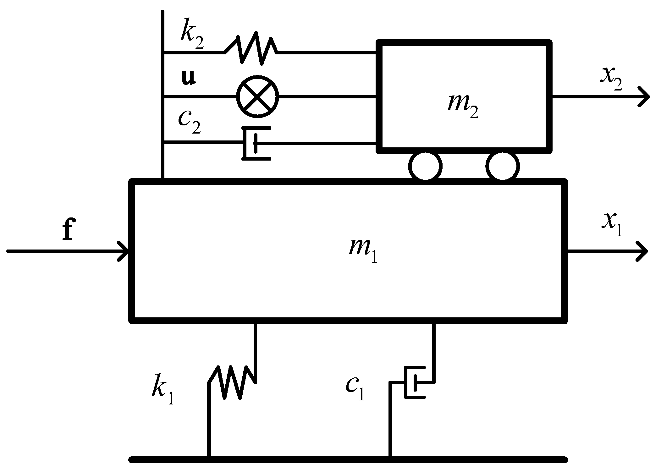
2.1. Active Mass Damper System of the Offshore Platform

The active mass damper (AMD) is the control device that suppresses structural vibration. It attaches the massive damper to the controlled structure to mitigate its harmful vibration by employing active forces properly. The steel jacket-type offshore platform with an AMD is described as a single-degree-of-freedom (SDOF) system, and the dominant layout for this SDOF system is shown in Figure 1 [24].
To explain the motion, the SDOF system is defined by Newton’s second law in [24,25]
m 1 ( t ) x ¨ 1 ( t ) + c 1 ( t ) x ˙ 1 ( t ) + k 1 ( t ) x 1 ( t ) c 2 ( t ) ( x ˙ 2 ( t ) x ˙ 1 ( t ) ) k 2 ( t ) ( x 2 ( t ) x 1 ( t ) ) = f ( t ) u ( t ) m 2 ( t ) x ¨ 2 ( t ) + c 2 ( t ) ( x ˙ 2 ( t ) x ˙ 1 ( t ) ) + k 2 ( t ) ( x 2 ( t ) x 1 ( t ) ) = u ( t )
where m 1 ( t ) , m 2 ( t ) , x 1 ( t ) , x 2 ( t ) , c 1 ( t ) , c 2 ( t ) , k 1 ( t ) and k 2 ( t ) are the mass, displacement response, stiffness coefficients and damping coefficients of the offshore structure and AMD device, respectively; f ( t ) is the disturbance acting on the structure, and u ( t ) is the control force provided by the AMD device. The vibration of the platform caused by f ( t ) should be stabilized with a properly designed u ( t ) , while perturbing c 1 ( t ) , c 2 ( t ) , k 1 ( t ) and k 2 ( t ) add uncertainty into the system. Using c 1 ( t ) and k 1 ( t ) as an example, the time-varying stiffness and damping are given by [24]
c 1 ( t ) = 2 m 1 ( t ) ξ 1 ( t ) ι 1 ( t ) , k 1 ( t ) = m 1 ( t ) ι 1 2 ( t )
where ξ 1 ( t ) = ξ 1 + ξ ^ 1 Δ ξ ˜ 1 ( t ) , ξ 1 represents the nominal value of the damping ratio; ξ ^ 1 stands for the maximum perturbation of the damping ratio; ι 1 ( t ) represents natural frequency, ι 1 ( t ) = ι 1 + ι ^ 1 Δ ι ˜ 1 ( t ) ; ι 1 represents the nominal value of the damping ratio; and ι ^ 1 stands for the maximum perturbation of the damping ratio. Here, ξ 1 ( t ) and ι 1 ( t ) share the limitations of t 0 , | Δ ξ ˜ 1 ( t ) | 1 and | Δ ι ˜ 1 ( t ) | 1 . Additionally, c 2 ( t ) and k 2 ( t ) share similar definitions, and we neglect the duplicates.
Inserting definition (2) into (1) yields
x ¨ 1 ( t ) + 2 ( ξ 1 ι 1 + ξ 1 ι ^ 1 Δ ι ˜ 1 ( t ) + ι 1 ξ ^ 1 Δ ξ ˜ 1 ( t ) ) x ˙ 1 ( t ) + ( ι 1 2 + 2 ι 1 ι ^ 1 Δ ι ˜ 1 ( t ) ) x 1 ( t ) 2 m 2 ( t ) ( ξ 2 ι 2 + ξ 2 ι ^ 2 Δ ι ˜ 2 ( t ) + ι 2 ξ ^ 2 Δ ξ ˜ 2 ( t ) ) ( x ˙ 2 ( t ) x ˙ 1 ( t ) ) / m 1 ( t ) + u ( t ) / m 1 ( t ) m 2 ( t ) ( ι 2 2 + 2 ι 2 ι ^ 2 Δ ι ˜ 2 ( t ) ) ( x 2 ( t ) x 1 ( t ) ) / m 1 ( t ) + g 1 ( t ) / m 1 ( t ) f ( t ) / m 1 ( t ) = 0 x ¨ 2 ( t ) + ( ι 2 2 + 2 ι ^ 2 ι 2 Δ ι ˜ 2 ( t ) ) ( x 2 ( t ) x 1 ( t ) ) u ( t ) / m 2 ( t ) + g 2 ( t ) / m 2 ( t ) + 2 ( ξ 2 ι 2 + ξ 2 ι ^ 2 Δ ι ˜ 2 ( t ) + ι 2 ξ ^ 2 Δ ξ ˜ 2 ( t ) ) ( x ˙ 2 ( t ) x ˙ 1 ( t ) ) = 0
with nonlinear parts
g 1 ( t ) = 2 m 1 ( t ) ι ^ 1 ξ ^ 1 Δ ι ˜ 1 ( t ) Δ ξ ˜ 1 ( t ) x ˙ 1 ( t ) m 2 ( t ) ι ^ 2 2 Δ ι ˜ 2 2 ( t ) ( x 2 ( t ) x 1 ( t ) ) + m 1 ( t ) ι ^ 1 2 Δ ι ˜ 1 2 ( t ) x 1 ( t ) 2 m 2 ( t ) ι ^ 2 ξ ^ 2 Δ ι ˜ 2 ( t ) Δ ξ ˜ 2 ( t ) ( x ˙ 2 ( t ) x ˙ 1 ( t ) ) g 2 ( t ) = m 2 ( t ) ι ^ 2 Δ ι ˜ 2 2 ( t ) ( x 2 ( t ) x 1 ( t ) ) + 2 m 2 ( t ) ι ^ 2 ξ ^ 2 Δ ι ˜ 2 ( t ) Δ ξ ˜ 2 ( t ) ( x ˙ 2 ( t ) x ˙ 1 ( t ) )
which are then defined as g ( t ) = [ g 1 ( t ) / m 1 ( t ) g 2 ( t ) / m 2 ( t ) ] T . Noting that the mass variables m 1 ( t ) and m 2 ( t ) are big enough, g ( t ) can be deleted from the motion equation.
The SDOF system (1) has a new form as
x ˙ ( t ) = ( A ( t ) + M ( t ) F ( t ) N ) x ( t ) + B ( t ) u ( t ) + D ( t ) f ( t )
where x ( t ) = [ x 1 ( t ) x 2 ( t ) x ˙ 1 ( t ) x ˙ 2 ( t ) ] T ,
A ( t ) = 0 0 ( ι 1 2 + ι 2 2 m 2 ( t ) / m 1 ( t ) ) ι 2 2 0 0 ι 2 2 m 2 ( t ) / m 1 ( t ) ι 2 2 1 0 2 ( ζ 1 ι 1 + ξ 2 ι 2 m 2 ( t ) / m 1 ( t ) ) 2 ξ 2 ι 2 0 1 2 ξ 2 ι 2 m 2 ( t ) / m 1 ( t ) 2 ξ 2 ι 2 T ,
M ( t ) = 0 0 ι ^ 1 0 0 0 ι ^ 2 m 2 ( t ) / m 1 ( t ) ι ^ 2 0 0 ξ ^ 1 0 0 0 ξ ^ 2 m 2 ( t ) / m 1 ( t ) ξ ^ 2 T ,
N = 2 ι 2 2 ι 2 0 0 0 2 ι 2 0 0 2 ξ 1 2 ξ 2 2 ι 1 2 ι 2 0 2 ξ 2 0 2 ι 2 T ,
B ( t ) = 0 0 1 / m 1 ( t ) 1 / m 2 ( t ) T ,
D ( t ) = 0 0 1 / m 1 ( t ) 0 T ,
F ( t ) = diag { Δ ι ˜ 1 ( t ) , Δ ι ˜ 2 ( t ) , Δ ξ ˜ 1 ( t ) , Δ ξ ˜ 2 ( t ) } satisfying F T ( t ) F ( t ) I , x ( t ) R m , u ( t ) R n , f ( t ) R p .

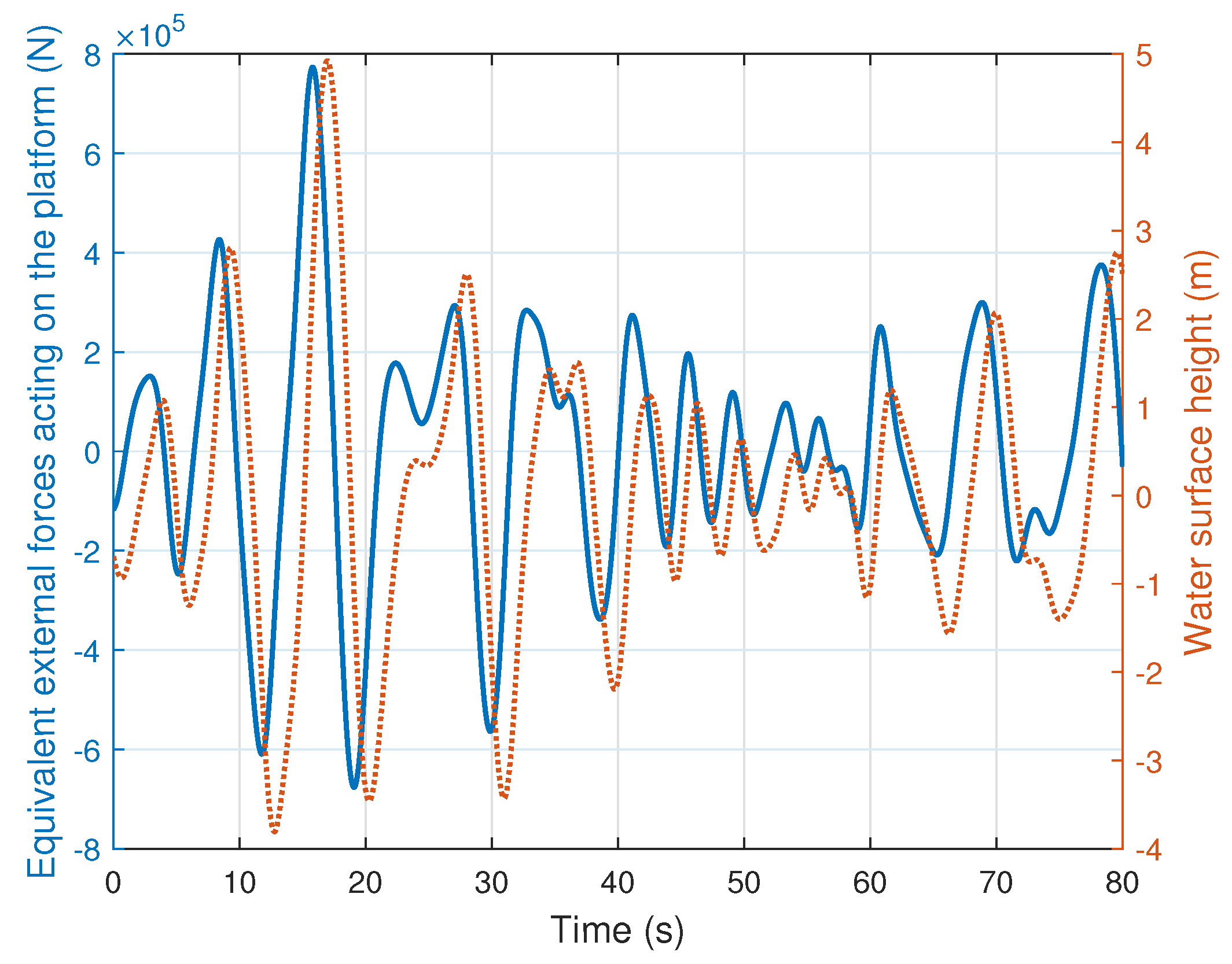
2.2. Loads Acting on the Platform

Ocean waves in conjunction with sea winds are the main excitation on the offshore platform. Wind loads usually account for around 20% of the whole external excitation, or even less in a calm wind field [24,26]. The statistical analysis of the environmental loads indicates that wind loads are usually neglected in a calm wind field. The description of waves is given by [24]
f j ( t ) = 0 d p j ( z , t ) φ ( z ) d z p j ( z , t ) = C d ρ D 8 / π σ v j v j ( z , d , t ) / 2 + C m ρ π D 2 v ˙ j ( z , d , t ) / 4 ϕ w a v e ( η ( t ) , C d , C m , D , ρ )
where f j ( t ) is the wave exciting force on the platform, and d is the water depth; p j is the wave load at the water depth z (zero at the bottom) generated from the Morison equation [24,25] via the function of water surface height η ( t ) , the diameter of equivalent pile cylinder D, the drag coefficient C d , the inertia coefficient C m and the fluid density ρ . Specifically, the velocity and acceleration of the water particle are
v j ( z , d , t ) = η ( t ) ω j c h ( k j z ) / s h ( k j d ) v ˙ j ( z , d , t ) = η ( t ) j ω j 2 c h ( k j z ) / s h ( k j d )
and σ v j is the standard deviation of v j at height z. For (7), k j is the wave number of the jth wave component in ω j 2 = g k j tanh ( k j d ) , g is the gravitational acceleration, j = 1 and ω j is the wave frequency. The wave height η ( t ) can be collected from practical experiments or generated based on wave spectra.
The above descriptions of wave disturbance rely on the basic component of the wave height η ( t ) . With a reliable wave spectrum, such as JONSWAP [27], we can restore the essential external force time series. The disturbance item is summarized
f ( t ) = 0 d ϕ w a v e ( η ( t ) , C d , C m , D , ρ ) φ ( z ) d z ϕ d i s ( η ( t ) )
based on (6) and (7), where ϕ d i s is a description function to be identified.

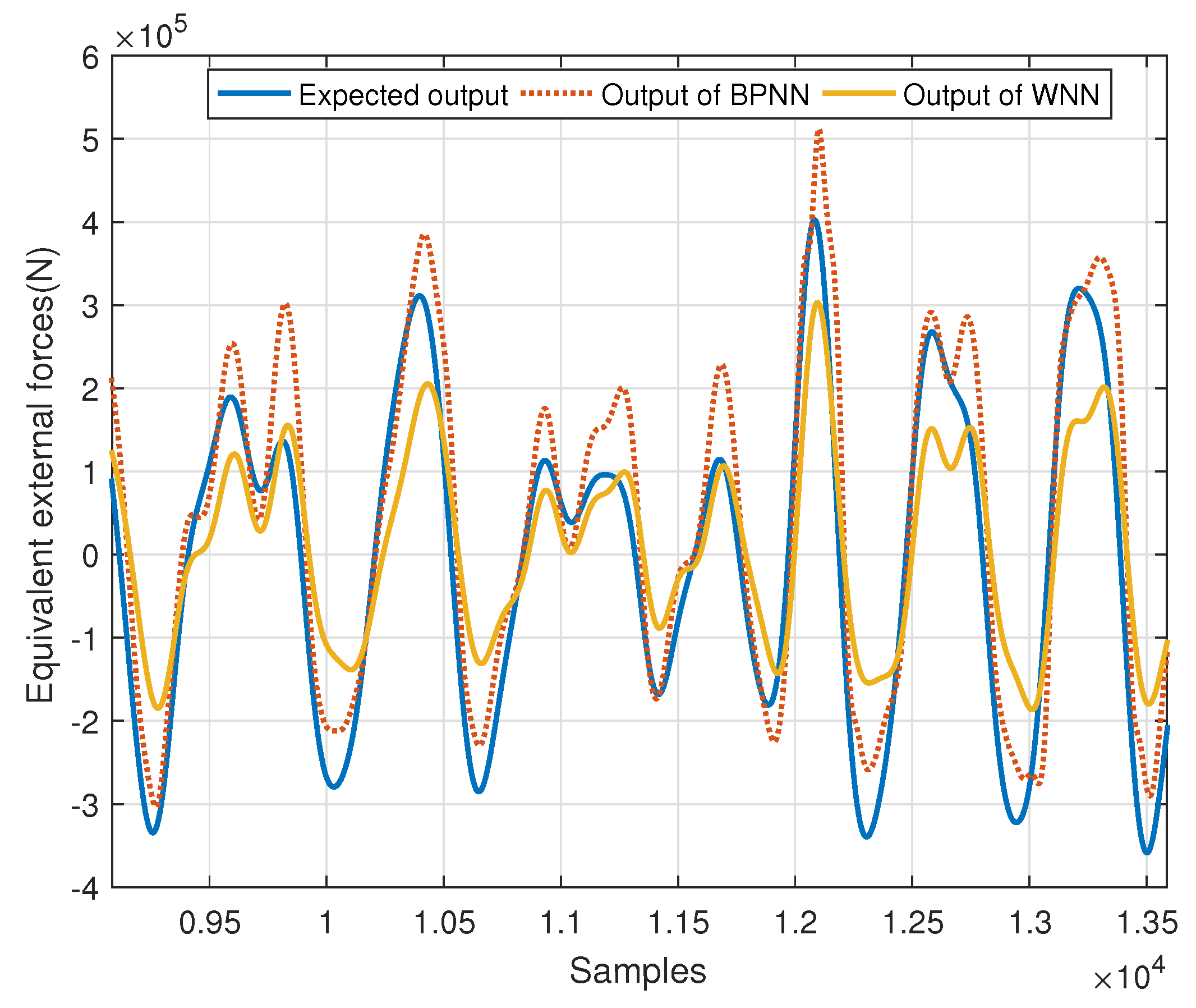
2.3. Data-Dependent Approximation of the Loads

Conventional methods for model identification require the determination of proper order and the recognition of separate weight values or the total matrices. Under the data-driven concept, we skip the acquisition procedure of the order and accurate real-time values. The learning input and output have more choices of dimensions and layers as the remedy for unknown orders and parameters. The disturbance function (8) is restored by a wavelet neural network [28,29], with the output defined as (9). The input layer has p 1 nodes with an input vector x i n , with available candidates x i n ( t ) = { η ( t ) , η ( t 1 ) , , y ( t ) , y ( t 1 ) , , x ( t ) , x ( t 1 ) , } . The hidden layer has l 1 nodes, and the output layer has n 1 nodes with an output vector y o u t . The weights ω i j between the hidden nodes and output nodes form the matrix W i j and obtain the output vector of the neural network
y o u t = W i j h ( x i n )
With the definition of the amplitude matrix a, transform matrix b, input weight matrix W j k and output of the wavelet function f w a v as h, the output of the hidden layer is
h ( x i n ) = f w a v ( W j k x i n b a ) f w a v ( x ¯ i n )
We choose the Morlet wavelet function as the active function [28]
f w a v ( x ¯ i n ) = e x ¯ i n 2 / 2 c o s ( 1.75 x ¯ i n )
and its derivative is
f w a v ( x ¯ i n ) = 1.75 s i n ( 1.75 x ¯ i n ) e x ¯ i n 2 / 2 x ¯ i n c o s ( 1.75 x ¯ i n ) e x ¯ i n 2 / 2
Define
E = 1 2 ( y i d e a l y o u t ) T ( y i d e a l y o u t ) 1 2 e T e
with the learning rates r 1 - r 4 , the updating laws for weights at the qth iteration are
W i j ( q + 1 ) = W i j ( q ) + Δ W i j ( q + 1 ) W j k ( q + 1 ) = W j k ( q ) + Δ W j k ( q + 1 ) a ( q + 1 ) = a ( q ) + Δ a ( q + 1 ) b ( q + 1 ) = b ( q ) + Δ b ( q + 1 )
which are illustrated by the gradient descent method based on (13)
Δ W i j ( q + 1 ) = r 1 E W i j ( q ) r 1 e h ( x ¯ i n ) Δ W j k ( q + 1 ) = r 2 E W j k ( q ) r 2 e W i j ( q ) f w a v ( W j k ( q ) x ¯ i n b ( q ) a ( q ) ) x ¯ i n ( a ( q ) ) 1 Δ a ( q + 1 ) = r 3 E a ( q ) r 3 e W i j ( q ) f w a v ( W j k ( q ) x ¯ i n b ( q ) a ( q ) ) ( W j k ( q ) x ¯ i n b ( q ) ) ( a ( q ) ) 2 Δ b ( q + 1 ) = r 4 E b ( q ) r 4 e W i j ( q ) f w a v ( W j k ( q ) x ¯ i n b ( q ) a ( q ) ) ( a ( q ) ) 1
When the neural network finishes the training on the given data set, the disturbance (8) identified by (9) after updates (14) and (15) will achieve the optimal weights W i j * , W j k * , a * and b * .

3. Main Results

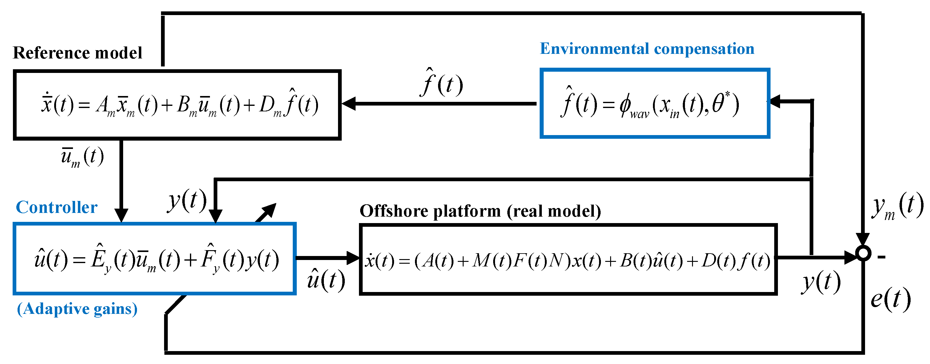
3.1. Environmental Compensation Scheme inside the Reference System

Define an environment-compensated reference model
x ˙ m ( t ) = A m x m ( t ) + B m u m ( t ) + D m f ^ m ( t ) y m ( t ) = C x m ( t )
where x m ( t ) , u m ( t ) , f ^ m ( t ) , y m ( t ) , A m , B m and D m are the references of x ( t ) , u ( t ) , f m ( t ) , y ( t ) , A ( t ) , B ( t ) and D ( t ) . The reference control input can be given by
u m ( t ) = R m 1 B m T P m x m ( t )
in which P m satisfies
A m T P m + P m A m + Q m = 0
with weight matrices of the cost function satisfying Q m > 0 and R m > 0 . The external disturbance f ^ m ( t ) is defined based on function ϕ d i s ,
f ^ m ( t ) = ϕ d i s ( x i n ( t ) , W i j * , W j k * , a * , b * )
where f ^ m ( t ) represents the item to restore the disturbance force f ( t ) , which is actually the f m ( t ) collected in the training set; x i n ( t ) = { η m ( t ) , η m ( t 1 ) , x m ( t ) , x m ( t 1 ) , y m ( t ) , y m ( t 1 ) } contains the reference inputs that are chosen for different approximation models, where η m ( t ) is related to f m ( t ) . The training of (8) approximated by (9) stops with
| | f ^ m ( t ) f m ( t ) | | < e m
where e m is a positive constant vector.
Based on the approximation model (19), the following theorem gives an adaptive compensated reference model control law with the structure assigned by Figure 2, where θ * represents the overall optimal hyperparameters W i j * , W j k * , a * , b * when the adaptive iteration finishes.

3.2. Model-Based Adaptive Controller Design

Theorem 1.
For the offshore platform (3), subject to random disturbance, choose a rough reference model stating
x ¯ ˙ m ( t ) = A m x ¯ m ( t ) + B m u ¯ m ( t ) + D m f ^ ( t ) y ¯ m ( t ) = C x ¯ m ( t )
where x ¯ m ( t ) and y ¯ m ( t ) are the reference states of x ( t ) and y ( t ) , and u ¯ m ( t ) is the reference control input
u ¯ m ( t ) = ( R ¯ m + B m T P ¯ m B m ) 1 B m T P ¯ m A m x ¯ m ( t )
in which P ¯ m is derived from
P ¯ m = A m T ( I + B m R ¯ m 1 B m T ) 1 P ¯ m A m + Q ¯ m
with R ¯ m > 0 , Q ¯ m > 0 . The environmental compensation model derived from (19) is replaced by
f ^ ( t ) = ϕ d i s ( x i n ( t ) , W i j * , W j k * , a * , b * )
where x i n ( t ) = { y ( t ) , y ( t 1 ) } contains the reference state input to be chosen in different approximation models. There exists an output feedback adaptive control law
u ^ ( t ) = E ^ y ( t ) u ¯ m ( t ) + F ^ y ( t ) y ( t )
which guarantees a stable system
x ˙ ( t ) = ( A ( t ) + M ( t ) F ( t ) N ) x ( t ) + B ( t ) u ^ ( t ) + D ( t ) f ( t ) y ( t ) = C x ( t )
where C decides the system output y ( t ) out of the system state x ( t ) with adaptive weights E ^ y ( t ) , and F ^ y ( t ) updating by
E ^ ˙ y T ( t ) = P ¯ y E 1 u ¯ m ( t ) e ¯ T ( t ) C P ¯ y e B m F ^ ˙ y T ( t ) = P ¯ y F 1 y ( t ) e ¯ T ( t ) C P ¯ y e B m
in which e ¯ ( t ) = y ¯ m ( t ) y ( t ) , P ¯ y F > 0 , P ¯ y E > 0 , P ¯ y e > 0 , and it is the solution of
A m T P ¯ y e + P ¯ y e A m + Q ¯ e = 0
where the quadratic weight matrix Q ¯ e satisfies Q ¯ e > 0 .
Proof. 
First, the reference control input (22) (which is another form of (17)) for (21) is derived from the quadratic cost function [23]
J = x ¯ m T Q m x ¯ m + u ¯ m T R m u ¯ m
It satisfies the stability conditions under the optimal theory with a maximum principle. The reference system (21), controlled by the reference control law (22), is stable.
Second, the compensated environmental disturbance requires the vibration response output of the rough reference model (16) and several features of the external disturbance in the form
f ^ m ( t ) = ϕ d i s ( x i n ( t ) , W i j * , W j k * , a * , b * )
The offline training should be performed on the historical data set with the goal (20). When the training completes, the real-time environmental loads will be approximated by the neural hyperparameters and the designated instant input. With regard to the same group of obtained neural hyperparameters, they are acquired by the training sample x i n ( t ) = { x m ( t ) , x m ( t 1 ) , y m ( t ) , y m ( t 1 ) } and f m ( t ) from (16) and then applied to output f ^ ( t ) using real x i n ( t ) = { x ( t ) , x ( t 1 ) , y ( t ) , y ( t 1 ) } from (26). Note that the state x ( t ) is not available in this situation together with η ( t ) and f ( t ) . Therefore, we should use x i n ( t ) = { y ( t ) , y ( t 1 ) } in both training and testing. The training period is adjusted with x i n ( t ) = { y m ( t ) , y m ( t 1 ) } . Given a non-negative constant vector e ϵ , the approximated f ^ ( t ) from (24) satisfies
| | f ^ ( t ) f ( t ) | | < e ϵ
which is the generalization goal of the neural network. It is achieved after numerical training [30,31].
Considering (5) and (16), the adjusting period of the adaptive weights should have the goal for the reference matrix D m and approximated loads f ^ ( t ) as
lim t D m f ^ ( t ) D ( t ) f ( t ) 0
It is noticed that real values for D ( t ) and f ( t ) are required for parameter correction, yet they are not given. There is no optimal value serving as the basis for approximation. As an alternative, the bound constraint of the parameters is given as follows for the proof of stability. Application with (31) and (32) added with a constant D , D ( t ) D satisfies
| | D m f ^ ( t ) D ( t ) f ( t ) | | | | ( D m D ) f ( t ) + D m e ϵ | |
Define the maximum disturbance load as f m a x , the bound constraint for (32) should be
| | D m D | | | | f ( t ) | | + | | D m | | | | e ϵ | | | | D m D | | | | f m a x | | + | | D m | | | | e ϵ | |
Each term on the right side of the above inequality is constant, which means there is an upper bound for (34). With the proper reference matrix D m , the adaptive law satisfies the premise (32).
Third, the error system between (3) and (26) is
e ˙ ( t ) = x ˙ m ( t ) x ˙ ( t ) = A m e ( t ) + [ A m A ( t ) M ( t ) F ( t ) N B ( t ) F ^ y ( t ) ] x ( t ) + [ B m B ( t ) E ^ y ( t ) ] u m ( t )
To realize the ideal approximating goal (36) with a positive constant matrix e c ,
lim t | | e ( t ) | | < e c
the adaptive weights should converge to the optimal E ^ y * ( t ) and F ^ y * ( t ) with
A m = A ( t ) + M ( t ) F ( t ) N + B ( t ) F ^ y * ( t ) B m = B ( t ) E ^ y * ( t )
Inserting (37) into (35) derives
e ˙ ( t ) = A m e ( t ) + B m E y * 1 ( t ) F ^ y ( t ) y ( t ) + B m E y * 1 ( t ) E ^ y ( t ) u ¯ m ( t )
with the deviation between the adaptive weights and the optimal weights defined by
F ˜ y ( t ) = F ^ y * ( t ) F ^ y ( t ) E ˜ y ( t ) = E ^ y * ( t ) E ^ y ( t )
(38) needs to satisfy the Lyapunov stability with the chosen function
V ( t ) = e T ( t ) P ¯ y e e ( t ) + tr ( F ˜ y T ( t ) P ¯ y F F ˜ y ( t ) ) + tr ( E ˜ y T ( t ) P ¯ y E E ˜ y ( t ) )
where P ¯ y e > 0 , P ¯ y F > 0 , P ¯ y E > 0 , satisfying V ( t ) > 0 . Using the derivative of (40) yields
V ˙ ( t ) = e T ( t ) ( A m T P ¯ y e + P ¯ y e A m ) e ( t ) + 2 tr [ F ˜ ˙ y T ( t ) P ¯ y F F ˜ y ( t ) + e T ( t ) P ¯ y e B m E y * 1 ( t ) F ˜ y ( t ) y ( t ) ] + 2 tr [ E ˜ ˙ y T ( t ) P ¯ y E E ˜ y ( t ) + e T ( t ) P ¯ y e B m E y * 1 ( t ) E ˜ y ( t ) u m ( t ) ]
Letting the last two items on the right side of (41) be zero, we have
tr [ F ˜ ˙ y T ( t ) P ¯ y F F ˜ y ( t ) + e T ( t ) P ¯ y e B m E y * 1 ( t ) F ˜ y ( t ) y ( t ) ] = 0 tr [ E ˜ ˙ y T ( t ) P ¯ y E E ˜ y ( t ) + e T ( t ) P ¯ y e B m E y * 1 ( t ) E ˜ y ( t ) u m ( t ) ] = 0
Inserting (39) into (42) derives the updating rules
F ˜ ˙ y T ( t ) = P ¯ y F 1 y ( t ) e T ( t ) P ¯ y e B m E y * 1 ( t ) E ˜ ˙ y T ( t ) = P ¯ y E 1 u m ( t ) e T ( t ) P ¯ y e B m E y * 1 ( t )
Noticing that there is no optimal value E y * 1 ( t ) , we set E y * 1 ( t ) = I as the substitute. Additionally, e ( t ) is not available as we assume when using y ( t ) (output feedback), instead of x ( t ) (state feedback), in the control environment. In this case, we use a rough replacement in the adaptive law in
F ˜ ˙ y T ( t ) = P ¯ y F 1 y ( t ) e ¯ T ( t ) P ¯ y e B m E ˜ ˙ y T ( t ) = P ¯ y E 1 u m ( t ) e ¯ T ( t ) P ¯ y e B m
and expect the adaptive rules to compensate this inaccurate setting of E y * and e ¯ ( t ) . Additionally, the exchange from e ( t ) to e ¯ ( t ) leads to a mismatch between the dimensions of e ¯ ( t ) and P ¯ y e . The proper weight matrix C is added in
F ˜ ˙ y T ( t ) = P ¯ y F 1 y ( t ) e ¯ T ( t ) C P ¯ y e B m E ˜ ˙ y T ( t ) = P ¯ y E 1 u m ( t ) e ¯ T ( t ) C P ¯ y e B m
Inserting (39) into (45) yields the rules for adaptive weights in (27).
Finally, the non-zero part left in (41) with the quadratic weight matrix Q ¯ e > 0 satisfies (28). It is easy to obtain the qualified P ¯ y e , and the control performance of the rules (45) with P ¯ y e replaced by P ¯ m is given in the simulation. Therefore, (41) obtains V ˙ ( t ) < 0 , and (38) is stable. This ends the proof. □

4. Numerical Results and Discussions

We conduct several simulation experiments on the offshore platform located in Gulf of Mexico described in Table 1 [32,33]. All the numerical tests use MATLAB as the simulating tool on CPU AMD Ryzen 7 4700U. The simulation duration is several minutes, and the sampling rate is 100 hz.

4.1. Simulating Verification of the Offshore Platform with Active Mass Damper to Suppress Vibration

The simulation model based on (3) in the marine environment (8) is materialized with the nominal values in Table 1. The wave description (6) is established by the JONSWAP spectrum [24]. We conduct a frequency analysis on the acceleration response of the platform, which is displayed in Figure 3. The blue line represents the vibration resulting from the wave loads, and the vibration controller settings for the yellow line will be introduced in the following subsections, together with the figures displaying the total vibration responses.
The two peaks indicate the governing vibration frequency of the platform. They are aligned with the peak frequency of the waves (0.79 rad/s) and the natural frequency of the platform (2.2 rad/s). The reduction in vibration is obvious when comparing the two lines, indicating the effectiveness of the proposed controller to be specified as follows.

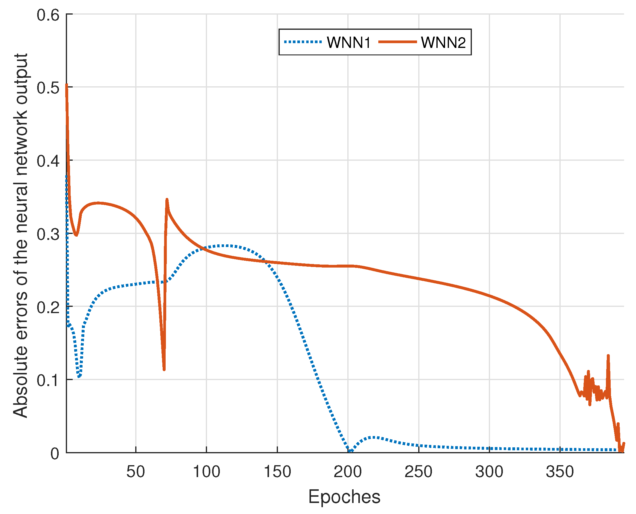
4.2. Adaptive Core and Reference Input Chosen for Disturbance Approximation

In the following section, the marine environment of the reference model concerning (21), (24) and (25) is estimated by (9). Two key points of the neural network are discussed in this section: the core neural function and the input.
Firstly, we should pick up a proper core neural network for the approximator. The Morlet wavelet function (11) is used as the active function when constructing the wavelet neural network (WNN). In comparison, the most common back-propagation neural network (BPNN) is activated with the sigmoid function in the hidden layer [34]. The training data set includes the equivalent force of external loads, and the wave surface height is reconstructed at a significant height 5.0 m [24]. Considering the available data on the disturbance, the input of the neural networks in this part is designated as η ( t ) , η ( t 1 ) , η ( t 2 ) , η ( t 3 ) , and the output is f ( t ) . Their numerical values during 80s are displayed in Figure 4. The two networks have 4-7-1 nodes, 3 × 10 4 training samples, maximum 800 epochs and 2 × 10 4 testing samples. Specifically, the test set is collected when the simulated wave’s significant height stays around 3.0 m, which means the fitting processes are different between the training and testing sets.
The proportion of the positive and negative values in the testing errors is shown in Table 2. The sum of the positive and negative proportions of each neural network should be 100% because we delete the zeros when counting the total. It is shown that the comparable BPNN has a drift in output. The testing output of BPNN is apparently biased towards the training data, which are bigger in value. The WNN keeps the same trend with the test data, with basically impartial positive and negative errors. Although the BPNN obtains smaller mean square errors in the output, as shown in Figure 5 (we display the samples between [ 0.9 × 10 4 , 1.4 × 10 4 ] for better illustration), the main object of this approximation period is to achieve a fair result during both training and testing. In that case, the WNN is more appropriate for our environmental compensation task.
Secondly, the approximator needs suitable input data. Different types of input for the neural network are discussed in this subsection, including the system state response x ( t ) , system output response y ( t ) , wave characteristics such as wave height η ( t ) , or the combination of multi-class data. The most common input for identifying external wave forces should be the wave height η ( t ) , as mentioned above, and we display the possible input η ( t ) and the defined output f ( t ) in Figure 4. Additionally, other possible inputs are x ( t ) and y ( t ) , and we list them in Figure 6.
We have constraints on the system (3) that no real-time disturbance data or full state data are available. Based on historical data sets including state samples and disturbance samples, we discuss the feasibility of different input. The sea surface height is theoretically more reliable as the input, as its approximation errors will not accumulate. The estimation at this time will not affect the next result, as a new η ( t ) is consistently given. In comparison, when the vibration response is used as the input of the approximation model, it will change the next approximation via the feedback part of the control law E ^ y ( t ) u ¯ m ( t ) . According to Figure 4 and Figure 6, we set two different neural networks, WNN1 and WNN2. The input of WNN1 is the sea surface height η ( t ) , and, for WNN2, the input is the vibration response y ( t ) . The comparison of the average error during each iteration is shown in Figure 7. It shows around 400 iterations in a possible simulation environment.
WNN1 represents the situation with qualified sensors to acquire wave features. WNN2 represents the limit that the disturbance monitoring sensors break down, and the approximation is totally dependent on the structural response of the platform itself. When the training is complete, both WNN1 and WNN2 obtain the desired estimation performance with a relatively small convergence error. Therefore, the vibration response output y ( t ) is proved reliable in the following experiments, satisfying the constraint of the state losses ( x ( t ) , f ( t ) and η ( t ) ) in the system.

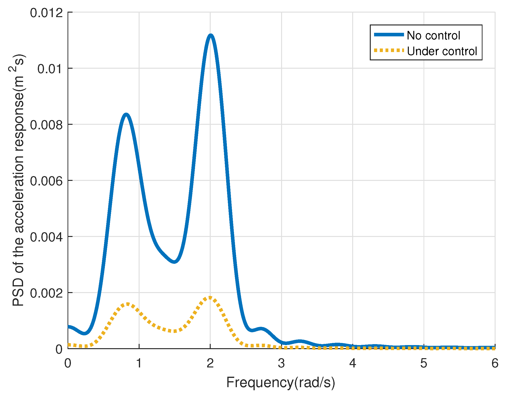
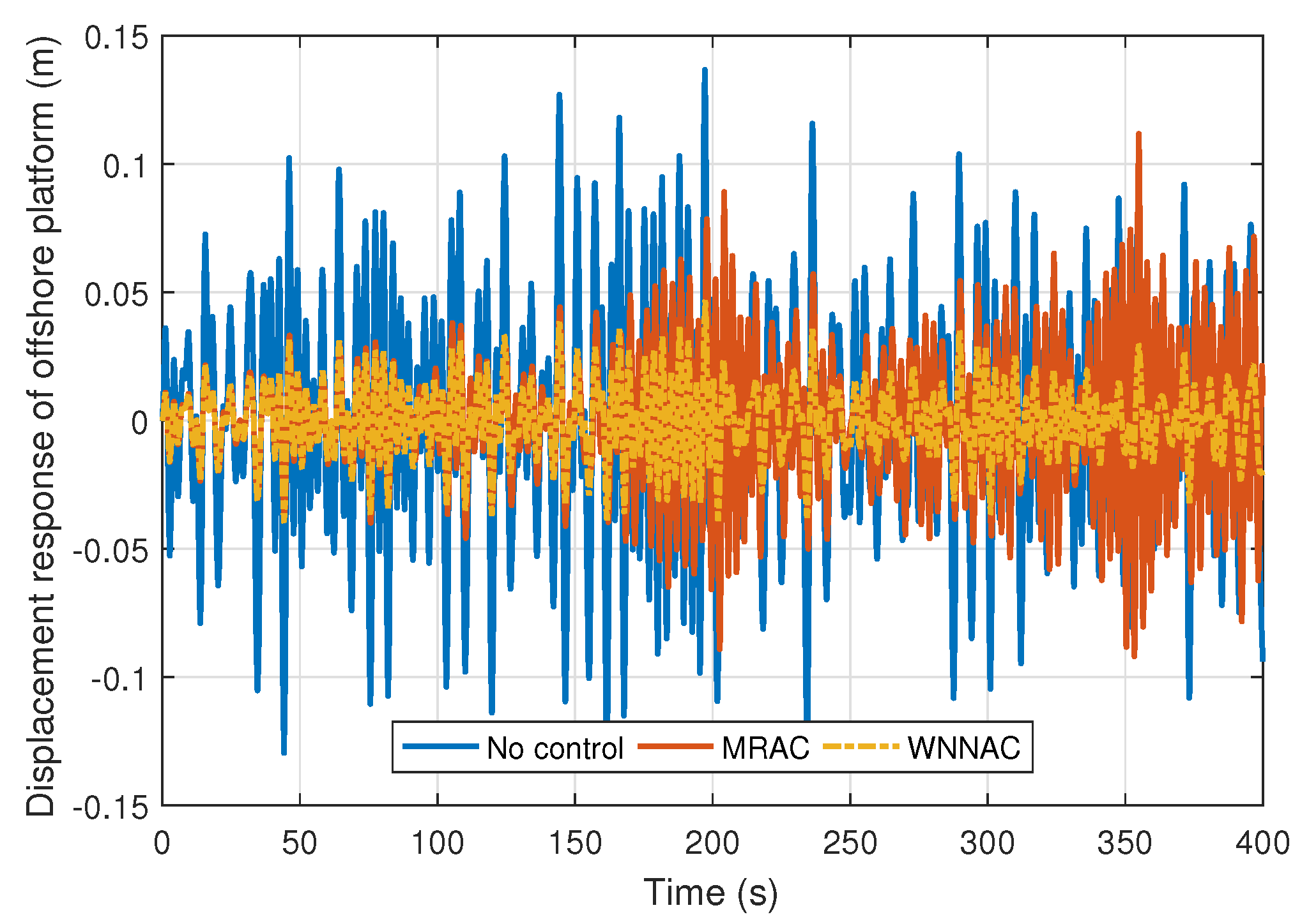
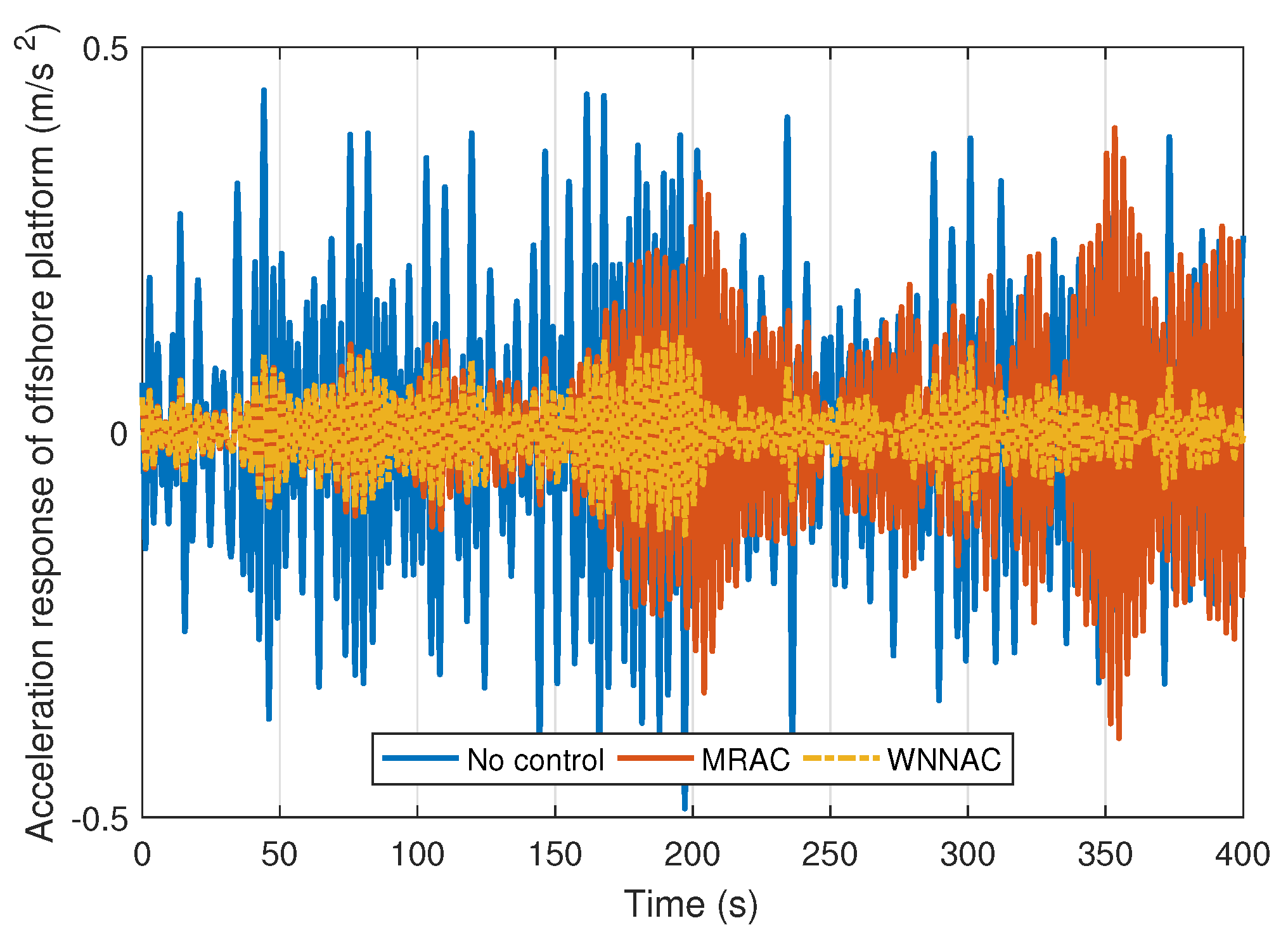
4.3. Controller Test Using Different Reference Models

In this subsection, the simulation model of the offshore platform to be controlled has unknown structural parameters. The nominal physical values are shown in Table 1, while each parameter has random perturbations. The discrete nominal parameters ( t = 0 ) are listed as follows.
A ( 0 ) + M ( 0 ) F ( 0 ) N = 0.9998 0 0.0100 0 0.0002 0.9994 0 0.0098 0.0423 0.0004 0.9988 0.0002 0.0400 0.0441 0.0083 0.9905 B ( 0 ) = 10 6 × 0 , 0.0006 , 0.0013 , 0.1272 T D ( 0 ) = 10 8 × 0.0006 , 0 , 0.1277 , 0.0005 T
  • Case 1. Control Performance with No. 1 Reference Model
In this case, (46) has 10% perturbations as { m 1 ( t ) ± 10 % , ι 1 ( t ) ± 10 % , ξ 1 ( t ) ± 10 % , m 2 ( t ) ± 10 % , ι 2 ( t ) ± 10 % and ξ 2 ( t ) ± 10 % }. Theoretically, any other platform model can be used as a reference model under the same settings of the governing mode. In this case, we use the features from another platform as the reference model [23]. Obviously, the platform height, water depth, mass and damping characteristics of the reference and the target platform models are different. The reference model with fixed nominal values is described by the following matrices in a discrete form.
A m = 0.9998 0 0.0100 0 0.0003 0.9997 0 0.0100 0.0486 0.0003 0.9980 0 0.0541 0.0542 0.0046 0.9954 B m = 10 6 × 0 , 0.0042 , 0.0042 , 0.8416 T D m = 10 8 × 0.0021 , 0 , 0.4215 , 0.0017 T
The control test is conducted in an ocean environment when the significant wave height stays at 5.0 m, with a comparable model reference adaptive controller (MRAC). We adopt the concepts [35,36] and assume that all of the information for the reference model is known. It has the adaptive law (25), in which the reference control input u ¯ m ( t ) is replaced by u m ( t ) in (17) on the basis of (16). The disturbance item f ^ ( t ) is replaced by the real value item f ( t ) , which means the limit for detection is quite strict. The wavelet neural network-based adaptive controller (WNNAC) is obtained via Theorem 1, together with an environmental compensation strategy (24), to replace (8), as shown in (21). In (29), we set Q m = 10 5 × diag { 1 , 0 , 1 , 0 } , R m = 10 4 for deriving (22). The other positive matrices are initially random. In short, the MRAC ideally knows all of the needed states and parameters, while the WNNAC needs approximations of certain information. The analysis of the responses is listed in Table 3 and Figure 8, Figure 9 and Figure 10, where S u , S x , S a and M u , M x , M a are the standard and maximum deviations, respectively.
Compared with the vibration response under uncontrolled conditions, the WNNAC can reduce the maximum displacement to 42.13%, the average deviation to 34.63%, the maximum acceleration deviation to 40.49% and the average deviation to 35.00%. The maximum control force provided by the WNNAC is 10.83% of that provided by the MRAC, and the average control force is 10.32%. In Figure 8 and Figure 9, the MRAC fails in a small range of around 350 s. For the first 300 s, the WNNAC has a 64.55% reduction in maximum control compared to the MRAC with a mean reduction of 73.96%. We only show 400 s in this simulation, and the total experiment lasts 16 min, with both controllers staying stable.
  • Case 2. Control Performance with Different Reference Models
In order not to lose the arbitrariness, we also test the WNNAC and MRAC when the reference model has random changes based on Case 1. For example, the element in the third row and first column of A m is 10 times the original value. B m has random changes at each element. The reference matrices are replaced by
A m = 0.9976 0 0.0100 0 0.0030 0.9997 0 0.0100 0.4859 0.0003 0.9958 0 0.0531 0.0542 0.0046 0.9954 B m = 10 6 × 0 , 0.0006 , 0.0013 , 0.1272 T
D m and the other settings are the same as in (47).
The vibration responses compared with the MRAC are displayed in Figure 11, Figure 12 and Figure 13. We can see that the WNNAC needs fewer control forces to achieve a control effect equivalent to that of the MRAC, and more details are displayed in Figure 12. The MRAC and WNNAC have basically the same reduction in the vibration responses, while the WNNAC has much smaller and more stable control forces in Figure 13.
Additionally, we test the WNNAC with the nominal values of m 1 ( t ) , ι 1 ( t ) , ξ 1 ( t ) , m 2 ( t ) , ι 2 ( t ) and ξ 2 ( t ) in the reference model and they have 0-60% random changes. The acceleration responses are shown in Figure 14 and details in Figure 15. The maximum perturbations of the reference model for each of the WNNACs are represented as 0 (blue line), 30%(red line) and 60%(yellow line). For example, the 60% perturbations are calculated by { m 1 ± 60 % , ι 1 ± 60 % , ξ 1 ± 60 % , m 2 ± 60 % , ι 2 ± 60 % , ξ 2 ± 60 % } in (47). The purple dashed line and the green dashed line define the perturbed scope of the acceleration response. Obviously, the WNNAC constrains the vibration response to a limited extent, which means changes in the chosen reference model are acceptable.

5. Conclusions

The adaptive control problem for offshore platforms subject to ocean loads is discussed in this paper. The simulation tests on the numerical model of the given platform prove that the proposed environmental compensating measures reduce more than half of the control forces compared to non-adaptive controllers. Moreover, the compensated reference system is able to be transferred among different perturbing systems. The potential aspect to optimize is in the rules to follow when selecting a proper reference model, including the proper sequences of different variables. We believe that there are many other reference models that can derive a stable adaptive controller for the target platform, and to what extent our environmental approximation measure maintains effectiveness could be investigated.

Author Contributions

Conceptualization, methodology, software, validation, writing—original draft preparation, Y.Z.; resources, data curation, writing—review and editing, H.M.; visualization, supervision, project administration, J.X.; formal analysis, funding acquisition, H.S.; investigation, J.Z. All authors have read and agreed to the published version of the manuscript.

Funding

This research was funded by the Natural Science Foundation of Shandong Province (Grants No. ZR2021MD054, ZR2017QF017) and the National Science Foundation of China (Grants No. 41276085).

Institutional Review Board Statement

Not applicable.

Informed Consent Statement

Not applicable.

Data Availability Statement

Not applicable.

Acknowledgments

This research was supported by the Ocean University of China.

Conflicts of Interest

The authors declare no conflict of interest.

References

  1. Erdogan, C.; Swain, G. The effects of biofouling and corrosion products on impressed current cathodic protection system design for offshore monopile foundations. J. Mar. Sci. Eng. 2022, 10, 1670. [Google Scholar] [CrossRef]
  2. Hemmati, A.; Oterkus, E. Semi-active structural control of offshore wind turbines considering damage development. J. Mar. Sci. Eng. 2018, 6, 102. [Google Scholar] [CrossRef] [Green Version]
  3. Yang, D.H.; Shin, J.H.; Lee, H.; Kim, S.K.; Kwak, M.K. Active vibration control of structure by Active Mass Damper and Multi-Modal Negative Acceleration Feedback control algorithm. J. Sound Vib. 2017, 392, 18–30. [Google Scholar] [CrossRef]
  4. Zhao, Y.D.; Sun, Y.T.; Zhang, B.L.; Han, Q.L.; Zhang, X.M. Recoil control of deepwater drilling riser systems via optimal control with feedforward mechanisms. Ocean. Eng. 2022, 257, 111690. [Google Scholar] [CrossRef]
  5. Zhang, W.; Zhang, B.L.; Han, Q.L.; Pang, F.B.; Sun, Y.T.; Zhang, X.M. Recoil attenuation for deepwater drilling riser systems via delayed H control. ISA Trans. 2022; in press. [Google Scholar] [CrossRef] [PubMed]
  6. Zhao, Y.D.; Sun, Y.T.; Zhang, B.L.; Zhang, D. Delay-feedback-based recoil control for deepwater drilling riser systems. Int. J. Syst. Sci. 2022, 53, 2535–2548. [Google Scholar] [CrossRef]
  7. Chen, Q.; Hu, Y.; Zhang, Q.; Jiang, J.; Chi, M.; Zhu, Y. Dynamic damping-based terminal sliding mode event-triggered fault-tolerant pre-compensation stochastic control for tracked ROV. J. Mar. Sci. Eng. 2022, 10, 1228. [Google Scholar] [CrossRef]
  8. Wu, D.; Chen, H.; Huang, Y.; Chen, S. Online monitoring and model-free adaptive control of weld penetration in vppaw based on extreme learning machine. IEEE Trans. Ind. Inform. 2019, 15, 2732–2740. [Google Scholar] [CrossRef]
  9. Calliess, J.P.; Roberts, S.J.; Rasmussen, C.E.; Maciejowski, J. Lazily Adapted Constant Kinky Inference for nonparametric regression and model-reference adaptive control. Automatica 2020, 122, 109216. [Google Scholar] [CrossRef]
  10. Gaudi, J.E.; Gibson, T.E.; Annaswamy, A.M.; Bolender, M.A.; Lavretsky, E. Connections between adaptive control and optimization in machine learning. In Proceedings of the IEEE 58th Conference on Decision and Control (CDC), Nice, France, 11–13 December 2019; pp. 4563–4568. [Google Scholar]
  11. Petković, D.; Danesh, A.S.; Dadkhah, M.; Misaghian, N.; Shamshirband, S.; Zalnezhad, E.; Pavlović, N.D. Adaptive control algorithm of flexible robotic gripper by extreme learning machine. Robot. Comput.-Integr. Manuf. 2016, 37, 170–178. [Google Scholar] [CrossRef]
  12. Cui, R.; Yang, C.; Li, Y.; Sharma, S. Adaptive control algorithm of flexible robotic gripper by extreme learning machine. IEEE Trans. Syst. Man Cybern. Syst. 2017, 47, 1019–1029. [Google Scholar] [CrossRef] [Green Version]
  13. Faradonbeh, M.K.S.; Tewari, A.; Michailidis, G. Input perturbations for adaptive control and learning. Automatica 2020, 117, 108950. [Google Scholar] [CrossRef] [Green Version]
  14. TOMIN, N.; KURBATSKY, V.; GULIYEV, H. Intelligent control of a wind turbine based on reinforcement learning. In Proceedings of the 2019 16th Conference on Electrical Machines, Drives and Power Systems (ELMA), Varna, Bulgaria, 6–8 June 2019; pp. 1–6. [Google Scholar]
  15. Frades, J.L.; Negro, V.; Barba, J.G.; Martín-Antón, M.; López-Gutiérrez, J.S.; Esteban, M.D.; Blasco, L.J.M. Preliminary design for wave run-up in offshore wind farms: Comparison between theoretical models and physical model tests. Energies 2019, 12, 492. [Google Scholar]
  16. Oliver, J.; Esteban, M.; López-Gutiérrez, J.S.; Negro, V.; Neves, M. Optimizing wave overtopping energy converters by ANN modelling: Evaluating the overtopping rate forecasting as the first step. Sustainability 2021, 13, 1483. [Google Scholar] [CrossRef]
  17. Liu, A.; Zhao, H.; Song, T.; Liu, Z.; Wang, H.; Sun, D. Adaptive control of manipulator based on neural network. Neural Comput. Appl. 2021, 33, 4077–4085. [Google Scholar] [CrossRef]
  18. Richmond, M.; Sobey, A.; Pandit, R.; Kolios, A. Stochastic assessment of aerodynamics within offshore wind farms based on machine-learning. Renew. Energy 2020, 161, 650–661. [Google Scholar] [CrossRef]
  19. Wu, J.; Xu, X.; Liu, C.; Deng, C.; Shao, X. Lamb wave-based damage detection of composite structures using deep convolutional neural network and continuous wavelet transform. Compos. Struct. 2021, 276, 114590. [Google Scholar] [CrossRef]
  20. Brito, M.; Bernardo, F.; Neves, M.G.; Neves, D.R.C.B.; Crespo, A.J.C.; Domínguez, J.M. Numerical model of constrained wave energy hyperbaric converter under full-scale sea wave conditions. J. Mar. Sci. Eng. 2022, 10, 1489. [Google Scholar] [CrossRef]
  21. Oh, J.; Suh, K.D. Real-time forecasting of wave heights using EOF-wavelet-neural network hybrid model. Ocean Eng. 2018, 150, 48–59. [Google Scholar] [CrossRef]
  22. Deshmukh, A.N.; Deo, M.C.; Bhaskaran, P.K.; Nair, T.M.B.; Sandhya, K.G. Neural-network-based data assimilation to improve numerical ocean wave forecast. IEEE J. Ocean. Eng. 2016, 41, 944–953. [Google Scholar] [CrossRef]
  23. Zhang, Y.; Ma, H.; Xu, J. Neural network-based fuzzy vibration controller for offshore platform with random time delay. Ocean Eng. 2021, 225, 108733. [Google Scholar] [CrossRef]
  24. Ma, H.; Zhang, Y.; Wang, S.Q.; Xu, J.; Su, H. Rolling-optimized model predictive vibration controller for offshore platforms subjected to random waves and winds under uncertain sensing delay. Ocean Eng. 2022, 252, 111054. [Google Scholar] [CrossRef]
  25. Chen, W.; Du, X.; Zhang, B.L.; Cai, Z.; Zheng, Z. Near-Optimal control for offshore structures with nonlinear energy sink mechanisms. J. Mar. Sci. Eng. 2022, 10, 817. [Google Scholar] [CrossRef]
  26. Jahangiri, V.; Sun, C. Three-dimensional vibration control of offshore floating wind turbines using multiple tuned mass dampers. Ocean Eng. 2020, 206, 107196. [Google Scholar] [CrossRef]
  27. Li, H.J.; Hu, S.L.J.; Jakubiak, C. H2 active vibration control for offshore platform subjected to wave loading. J. Sound Vib. 2003, 263, 709–724. [Google Scholar] [CrossRef]
  28. Sabir, Z.; Raja, M.A.Z.; Mahmoud, S.R.; Balubaid, M.; Algarni, A.; Alghtani, A.H.; Aly, A.A.; Le, D.N. A novel design of Morlet wavelet to solve the dynamics of nervous stomach nonlinear model. Int. J. Comput. Intell. Syst. 2022, 15, 1–15. [Google Scholar] [CrossRef]
  29. Yang, C.; Yang, R.; Xu, T.; Li, Y. Computational model of enterprise cooperative technology innovation risk based on nerve network. J. Algorithms Comput. Technol. 2018, 12, 177–184. [Google Scholar] [CrossRef]
  30. Chamon, L.; Ribeiro, A. Probably approximately correct constrained learning. Adv. Neural Inf. Process. Syst. 2020, 33, 16722–16735. [Google Scholar]
  31. Fang, Z.; Lu, J.; Liu, F.; Zhang, G. Semi-supervised heterogeneous domain adaptation: Theory and algorithms. IEEE Trans. Pattern Anal. Mach. Intell. 2022, 45, 1087–1105. [Google Scholar] [CrossRef]
  32. Ma, H.; Hu, W.; Tang, G.Y. Networked predictive vibration control for offshore platforms with random time delays, packet dropouts and disordering. J. Sound Vib. 2019, 441, 187–203. [Google Scholar] [CrossRef]
  33. Ma, H.; Tang, G.Y.; Ding, X.Q. Modified-transformation-based networked controller for offshore platforms under multiple outloads. Ocean Eng. 2019, 190, 1–11. [Google Scholar] [CrossRef]
  34. Chen, L.; Jagota, V.; Kumar, A. Research on optimization of scientific research performance management based on BP neural network. Int. J. Syst. Assur. Eng. Manag. 2021. [Google Scholar] [CrossRef]
  35. Su, G.; Wang, P.; Guo, Y.; Cheng, G.; Wang, S.; Zhao, D. Multiparameter identification of permanent magnet synchronous motor based on model reference adaptive system—Simulated annealing particle swarm optimization algorithm. Electronics 2022, 11, 159. [Google Scholar] [CrossRef]
  36. Aljuboury, A.S.; Hameed, A.H.; Ajel, A.R.; Humaidi, A.J.; Alkhayyat, A.; Mhdawi, A.K.A. Robust adaptive control of knee exoskeleton-assistant system based on nonlinear disturbance observer. Actuators 2022, 11, 78. [Google Scholar] [CrossRef]
Figure 1. Simplified SDOF model of the platform with AMD on deck (adapted from [24] with permission from Elsevier, 2022).
Jmse 11 00138 g001
Figure 2. Model reference adaptive vibration controller with compensated environment.
Jmse 11 00138 g002
Figure 3. Power spectral density on the acceleration response of the offshore platform.
Jmse 11 00138 g003
Figure 4. Ocean loads and wave height.
Jmse 11 00138 g004
Figure 5. Comparison of the approximation models using different neural networks.
Jmse 11 00138 g005
Figure 6. Ocean loads and displacement response of the platform.
Jmse 11 00138 g006
Figure 7. Comparison of the approximation models using different inputs.
Jmse 11 00138 g007
Figure 8. Displacement response of the offshore platform structure.
Jmse 11 00138 g008
Figure 9. Acceleration response of the offshore platform structure.
Jmse 11 00138 g009
Figure 10. Control force to suppress the vibration.
Jmse 11 00138 g010
Figure 11. Acceleration response of the offshore platform structure using another reference model.
Jmse 11 00138 g011
Figure 12. Acceleration response of the offshore platform structure (details).
Jmse 11 00138 g012
Figure 13. Control force to suppress the vibration using another reference model.
Jmse 11 00138 g013
Figure 14. Control force to suppress the vibration with different perturbations in platform parameters.
Jmse 11 00138 g014
Figure 15. Control force to suppress the vibration with different perturbations in platform parameters (enlarged view of Figure 13).
Jmse 11 00138 g015
Table 1. Parameters of offshore platform and sea condition.
DescriptionSymbolValueUnit
Significant wave height H s 5m
Peak frequency ω 0 0.79rad/s
Water depthd218m
Pile cylinderD1.83m
Height of platformL249m
First modal mass m 1 7,825,307kg
Nominal value of natural frequency (platform) ι 1 2.0446rad/s
Nominal value of damping ratio (platform) ξ 1 2%-
AMD device mass m 2 78,253kg
Nominal value of natural frequency (AMD) ι 2 2.0074rad/s
Nominal value of damping ratio (AMD) ξ 2 20%-
Drag coefficient C d 1.0-
Inertia coefficient C m 1.5-
Atmospheric density ρ ¯ 1.23-
Windward resistance coefficient C H 1.01-
Table 2. The proportion of output error from different neural networks.
Positive ErrorsNegative Errors
BPNN80.77%Less than 20%
WNN61.79%38.21%
Table 3. Numerical analysis of the vibration response of the offshore platform.
S u ( 10 4 N ) S x (m) S a ( m / s 2 ) M u ( 10 4 N ) M x (m) M a ( m / s 2 )
No control-0.04360.1317-0.11820.3818
MRAC14.7850.05710.236571.9960.24500.9797
MRAC(1-300s)5.85860.02370.088321.3880.08910.3379
WNNAC1.52570.01510.04617.58210.04980.1546
Disclaimer/Publisher’s Note: The statements, opinions and data contained in all publications are solely those of the individual author(s) and contributor(s) and not of MDPI and/or the editor(s). MDPI and/or the editor(s) disclaim responsibility for any injury to people or property resulting from any ideas, methods, instructions or products referred to in the content.

