

Water Exchange Due to Wind and Waves in a Monsoon Prevailing Tropical Atoll

Taiwan Ocean Research Institute, National Applied Research Laboratories, Kaohsiung City 852, Taiwan
J. Mar. Sci. Eng. 2023, 11(1), 109; https://doi.org/10.3390/jmse11010109
Submission received: 25 November 2022
/
Revised: 30 December 2022
/
Accepted: 2 January 2023
/
Published: 5 January 2023
(This article belongs to the Special Issue Hydrodynamic Circulation Modelling in the Marine Environment)
Abstract
:Physical forcings affect water exchange in coral reef atolls. Characteristics of the consequent water exchange depend on the atoll morphology and the local atmospheric and hydrographic conditions. The pattern of water exchange at the Dongsha atoll under the influences of tides, wind, and waves was investigated by conducting realistic modeling and numerical experiments. The analyses suggest that the southwestern wind could enhance the inflow transports at the southern reef flat and the outflow transports at the northern reef flat/north channel. The northeastern wind induces an inversed pattern. Unlike the wind, the waves always strengthen the inflow transports at the reef flat, and the locations of strengthened transports depend on the incident directions of the waves. Wind and waves induce shorter hydrodynamic time scales than tides, suggesting more vigorous water exchange during high wind and waves. The directions of wind and waves significantly affect the spatial distributions of the residence time and the age. This implies that the hydrodynamic processes in the Dongsha Atoll would have significant seasonal variability. This study presents different circulation patterns in an atoll system influenced by calm weather and strong wind/waves.
1. Introduction
Unlike fringing and barrier reefs that reside on the shorelines of lands, coral reef atolls rise solely in the deep ocean. They exhibit simple or irregular geometries, and their morphology generally includes steep fore reefs, reef flats, a lagoon, and several passes connecting the lagoon and the open ocean. The reef flats can be submerged or partly emerged with vegetation or residents on them. Passes can be channels of several kilometers wide or narrow leakages of several meters wide. The saucer-shaped lagoon exchanges its water with the open ocean through the passes and over the reef flats. For example, the Bikini Atoll, which is well known for the nuclear tests conducted there between 1946 and 1958, has a central lagoon enclosed by reef flats, islands, several narrow passes with an accumulation of width of about 3 km, and two wide channels in the south with widths of 3.5 and 15.7 km. The water exchange occurs through the passes and the reef flats [1].
Coral reef atolls build ecosystems with high biodiversity in the nutrient-poor open ocean. The ecosystems are strongly influenced by the nutrient concentrations and water qualities of the atolls, greatly depending on the water exchange with the open ocean. For example, the degree of water exchange determines either nitrogen or phosphorus limitations in an atoll lagoon; nitrogen limitation was found in large and open atoll lagoons, and phosphorus limitation was found in shallow and enclosed atoll lagoons [2]. As a result, understanding the processes of water exchange in an atoll could help us gain a better understanding of the atoll ecosystem.
The water exchange in atolls is controlled by hydrodynamic forcings, such as waves, tides, and wind [3]. Surface waves are considered the primary driving force for flows over the reef flats in many reef–lagoon systems [3]. The mechanism is that, as the incident waves break on the fore reefs, the breaking causes water setup, providing pressure gradient for outside waters across the reef flat into the lagoon [4,5,6,7,8]. Lowe et al. [7] collected field data in Kaneohe Bay, Hawaii, and found that wave forcing dominated the circulations. Their data roughly matched the theoretical prediction of wave-driven currents, which incorporated radiation stresses, setup gradients, bottom friction, and the morphological properties of the reef–lagoon system. For the atolls, Callaghan et al. [8] conducted measurements in two atolls in the South Pacific and found that, although the lagoon water level was above the surrounding sea level, flushing still occurred and was driven by waves pumping water over the reef flat into the lagoon.
Tides provide periodic and relatively predictable forcing to the water exchange between the lagoon and the open ocean. Due to the nature of alternating flushing, tides are considered a weaker driving force to water renewal than waves [8]. However, tides can be powerful in driving water exchange in the presence of narrow passes in atolls. Dumas et al. [9] found that tides can generate strong currents through the narrow passage at the Ahe atoll and create jet-like residual circulations in the lagoon. Tides also modulate wave-driven currents by affecting the wave breaking in different tidal phases [10,11]. In regions with large tidal ranges, the offshore water level drops below the reef rim during low tides, and the exposed reef becomes a barrier to water pumping into the lagoon by waves [12].
Wind forcing is known for its influence on lagoon circulations [9,13,14,15,16,17]. Two-layer circulations due to wind are observed in lagoons where wind drives shallow lagoon water aligned with the wind direction; consequently, deep water flows backward due to the continuity [9,13]. Depending on the morphology of atolls, there may be lagoon circulations which trap water from exporting to the open ocean [14]. Wind can directly impose wind stresses to drive shallow water on reef flats, and it also induces piled-up sea levels which result in pressure gradient flows. In a one-dimensional aspect of momentum balance, the authors of [18] related the wind-driven transport on the reef flats to the wind stress, the cross-reef spatial variation of sea level, and the bottom friction. Since reef flats usually cover a sizable portion of the atoll boundary between the lagoon and the open ocean, wind-driven over-reef currents are potentially dominant for water exchange in atolls.
In this study, I use Dongsha Atoll as an example to study the tide-, wind-, and wave-driven exchange processes between the lagoon and the open ocean. Many studies about Dongsha Atoll have focused on topics of internal waves and their implications ([19,20,21,22,23,24]); however, to my best knowledge, there is no model study about the circulations inside the Dongsha Atoll. A current–wave coupled model, COAWST, which is widely used in studies about current–wave interactions in several regions (e.g., [25,26,27]; see Section 2.2 for details of the model) with realistic atoll bathymetry, atmospheric, and oceanic conditions, was built, and numerical experiments were conducted to investigate the processes of water exchange in the Dongsha Atoll.
The paper is organized as follows: in Section 2, the study site, period, and model setup are described. The transports across boundaries between the lagoon and the open ocean are analyzed and discussed in Section 3. The methods of tracer and float tracking are used to assess the efficiency of water exchange in Section 4. The conclusions of the study are given in Section 5.
2. Methods
2.1. Study Site and Period
The study site is at the Dongsha Atoll, a tropical coral reef atoll located at the edge of the shelf in the northern South China Sea (Figure 1a). It emerges from the seafloor at about 500 m depth and forms a circular-shaped coral reef atoll with a diameter of about 25 km. A reef flat, which is submerged in shallow water of about 1 m, encloses the central lagoon in the north, east, and south (Figure 1b). The general cross-shore width of the reef flat is about 2 km. In the west, Dongsha Island is located between the north channel and the south channel. The two channels, with depths of approximately 8 m and widths of approximately 5 km (north) and 10 km (south), are the main passages connecting the lagoon and the surrounding open ocean. The central lagoon is saucer-shaped, and only 2% of the area is deeper than 16 m.
I selected the period for the modeling study to partly coincide with the period of the mooring observations carried out by a research group at Taiwan Ocean Research Institute in August/September 2021 so as to have measurement data to validate the model (sites H10 and N09 in Figure 1c). The atmospheric and wave conditions during the study period are shown in Figure 2. The data source of the atmospheric conditions was ECMWF ERA5 [28], and the significant wave height was derived from the global wave system MFWAM performed by Météo-France (retrieved from CMEMS; https://data.marine.copernicus.eu/product/GLOBAL_ANALYSISFORECAST_WAV_001_027/description; accessed on 4 January 2023). These time series are the data interpolated to 117° E, 20.7° N, about 10 km east of the Dongsha. The wind speed was less than , and directions changed frequently most of the time, except for a strong windy event that occurred during 21 July and 17 August (Figure 2a). Wind speed increased by on 5 August and decreased by on 17 August. During this event, a southwest wind prevailed, denoting the typical summer monsoon in the northern South China Sea. The enhanced wind caused increases in the significant wave height from a calm wave condition of about 1 m to 4 m on 5 August when the wind speed peaked at (Figure 2b). The waves then dropped to calm conditions at the end of the event. Regarding the net heat flux, the diurnal cycle was dominant with maximum values in the daytime. The daytime net heat fluxes were higher than 500 on the sunny days and dropped significantly on the rainy days (Figure 2c,d).
2.2. The Realistic Model
To study the water exchange processes driven by physical forcings, especially wind and waves, I adopted the coupled ocean–atmosphere–wave–sediment transport modeling system, COAWST v3.7 [29], to build an ocean circulation model coupled with a wave model for the Dongsha Atoll and the surrounding sea. The ocean circulation component of COAWST is the Regional Ocean Modeling System (ROMS v3.9) [30,31], and the wave component is the Simulating Waves Nearshore system (SWAN v41.31) [32,33]. The ROMS is a three-dimensional, free-surface, terrain-following, hydrostatic primitive equation model and is especially capable of modeling circulations in coastal and estuarine regions. The SWAN is a third-generation wave model based on the wave action balance equation with a variety of sources and sinks (see Appendix A for governing equations of ROMS and SWAN). The SWAN provides wave parameters (e.g., wave height, length, period, and dissipations) to the ROMS to implement the vortex force that represents the wave–current interactions [34]. In response, the ROMS provides surface currents and sea levels to the SWAN for modifying wind speed forcing and wave propagation.
The bathymetry data in the model were a composite of two datasets; the bathymetry data inside the atoll were derived from the data used for navigation by the Dongsha Atoll Research Station, and the bathymetry data in the open ocean were interpolated from ETOPO1 [35] (retrieved from https://www.ngdc.noaa.gov/mgg/global/; accessed on 4 January 2023). For the ROMS, a Cartesian grid system with 600 400 grids on longitude and latitude (spanning 116.2–117.2° E, 20.4–21° N; Figure 1b) and 20 terrain-following vertical levels were set for the model. The horizontal grids were stretched toward the Dongsha Atoll, giving a minimum grid size of ~110 m in the atoll lagoon and a maximum of ~320 m near the corners of the model domain. In general, the mean grid size within the atoll was ~120 m. A time step of baroclinic (slow) mode was set to 10 s, and there were 20 barotropic (fast) steps between successive baroclinic steps.
The ROMS was driven by realistic, time-varying atmospheric and oceanic conditions. For the initial conditions and lateral open boundary conditions, I provided three-dimensional and two-dimensional velocities, free surface height, temperature, and salinity, which were interpolated from the 1/12 three-hourly output of HYCOM GOFS 3.0 Global Analysis (retrieved from https://www.hycom.org/dataserver/gofs-3pt1/analysis; accessed on 4 January 2023). The scheme of boundary conditions for free surface height and two-dimensional velocities was based on [36,37], respectively. For three-dimensional velocities, temperature, and salinity, the radiation-nudging boundary condition was applied. I also superimposed the tidal levels and tidal currents, which were based on the 1/30 TPXO8-atlas [38] (retrieved from https://www.tpxo.net/global/tpxo8-atlas; accessed on 4 January 2023), on the open boundary conditions to introduce tidal forcing containing 13 tidal constituents, Q1, O1, P1, K1, N2, M2, S2, K2, Mf, Mm, M4, Ms4, and MN4. At the sea surface, the atmospheric forces derived from three-hourly ECMWF ERA5 were applied, and the ROMS built-in bulk parameterization scheme, based on COARE 3.0 [39], was utilized to provide surface momentum, heat, and water fluxes.
In ROMS, a third-order upstream-biased scheme was used for three-dimensional momentum advection and horizontal tracer advection (temperature and salinity), and a fourth-order centered scheme was used for two-dimensional transport and vertical tracer advection. The harmonic horizontal viscosity coefficients for momentum and diffusion coefficient for tracers were set to 1 . Turbulent vertical mixing for both momentum and tracers was computed using the -epsilon turbulent closure in the form of generic length-scale scheme (GLS).
To parameterize the friction of the seafloor in the atoll, the classical law-of-the-wall logarithmic velocity profile,
was assumed for the first vertical grid above the bottom, where is the velocity at the first vertical grid , is the friction velocity, is the von Kármán constant equal to 0.41, and is the roughness length. On the basis of Equation (1), the bottom friction is given, where is a background density. The drag coefficient is, thus, . In this formulation, is the only unknown parameter. Although spatially variable reflects different types of bottom materials, such as corals, seagrasses, or sediments [40], reef-lagoon models can perform well with spatially uniform parameters of bottom friction by carefully assessing the parameters [17]. I tested several values of , and chose cm. This value approximates the results reported by [18] for the reef flat of the Dongsha Atoll, although their formulation of the logarithmic profile contains an additional term accounting for the effects of wakes, which is absent from our formulation.
The SWAN component ran in the third-generation mode for wind input, quadruplet interactions, and whitecapping. It used the same modeling domain, bathymetry, and wind forcing as ROMS. The wave growth scheme was adopted from [41] (SWAN command GEN3 KOMEN). The whitecapping according to [41] was applied (SWAN command WCAPPING KOMEN 2.36E-5 3.02E-3 2.0 1.0 1.0). The wave initial condition was acquired through a stationary run of SWAN with the initial wind fields. Then, SWAN was integrated with a timestep size of 5 min and interchanged data with the ROMS component every 10 min. The boundary conditions of waves were interpolated from the CMEMS , three-hourly wave product MFWAM (see Section 2.1). The waves were attenuated by bottom friction in the form of [42] with the bottom roughness length scale of 1 m (SWAN command FRICTION MADSEN 1.0). A constant breaker index was employed, where the ratio of maximum individual wave height over water depth was set to 0.73 (SWAN command BREAKING CONSTANT 1.0 0.73).
This realistic coupled modeling was integrated from 1 July to 29 September 2021 (90 days). For the purpose of spin-up, the modeled outputs after 00:00 on 10 July were analyzed.
2.3. Numerical Experiments
In addition to the realistic modeling, I designed numerical experiments with simplified forcings, trying to isolate the effects of tides, wind, and waves on water exchange. The baseline experiment was driven by tides only. According to harmonic analysis, the dominant tidal constituents were K1, O1, and M2 in the Dongsha Atoll (not shown here). For simplicity, I drove an initially quiescent experiment using homogeneous K1 tidal levels and currents on the open boundaries as the baseline experiment (denoted by T). Then, wind and wave forcings were added to the baseline experiment separately. Since Dongsha Atoll is located in a monsoon-prevailing region, the experiments were designed to mimic the summer and winter monsoons, corresponding to southwestern wind and northeastern winds, respectively. As a result, a kinematic surface momentum flux of 0.23 (corresponding to a wind speed of about 14 ) in the southwest and northeast directions was applied to the baseline experiment T, denoted by TWi_SW and TWi_NE, respectively. Although the wind is the source of surface waves, I isolated the effects of waves by designing experiments driven by wave forcing only. To solely add wave forcing to the baseline experiment T, two SWAN runs driven by southwestern (denoted by TWa_SW) and northeastern (denoted by TWa_NE) 14 winds were coupled with the experiment T, from which the wind forcing in the ROMS was absent. The high wind speed generated an incident significant height of about 2.4 m, about 10 km away from the reef edge of the Dongsha Atoll. A summary of these numerical experiments is shown in Table 1.
2.4. In Situ Measurements
The model was validated against the in situ measurements conducted by members of Taiwan Ocean Research Institute, National Applied Research Laboratories. Two 600 kHz Teledyne RDI Workhorse Sentinel ADCPs were deployed in the lagoon of Dongsha Atoll at depths of 7.5 m (H10) and 9.2 m (N09) (see Figure 1c) to collect surface elevations, current velocities, and wave parameters. The ensemble interval for surface elevations and current velocities was set to 300 s, and the bin size was 0.35 m (first bin range: 1.43 m). The wave measurements were carried out with a burst mode with a sample rate of 2 Hz in 10 min, and the time between bursts was 60 min.
3. Results
3.1. Model Validation
The comparisons of simulated and observational surface elevation, eastward and northward depth-averaged velocities, significant wave height, and peak wave period are shown in Figure 3a,b for site H10 and N09, respectively. To assess model performance quantitatively, I adapted the skill score (SS), Pearson correlation coefficient (), root-mean-square error (RMSE), and bias. The skill score [43] is expressed as
where denotes the hourly model outputs, denotes the observations, is the total number of data, and the angle brackets denote averaging over the data. The maximum value of SS is 1, representing that the model outputs and the observations are the same. The Pearson correlation coefficient is calculated by
A perfect relationship between the model and observations has an value of 1, no relationship is represented by 0, and a perfect negative relationship leads to a value of −1. The root-mean-square error is calculated by
The root-mean-square error measures variance between the model and the observations. Bias is calculated by
Bias indicates whether the model, on average, overestimates (positive) or underestimates (negative) the observations. The corresponding performance metrics are listed in Table 2. In Figure 3, the modeled and the observational surface elevations agree well with SS of 0.99 and at the two sites, indicative of the precise surface-elevation simulation of the model. This suggests that the tidal amplitude and phase were correctly modeled. In terms of depth-averaged velocities, the tidal current was well reproduced by the model at H10 (Figure 3a) with (eastward depth-averaged velocity) and (northward depth-averaged velocity). At N09, for eastward depth-averaged velocity and for northward depth-averaged velocity, which were apparently lower than those at H10. However, the tidal variations were still correctly modeled, as shown in Figure 3b. At H10, larger discrepancies appeared in the comparison of eastward velocity after 26 August, but the modeled northward velocity showed consistent variations with the observations. At N09, both modeled eastward and northward velocities appeared to have different tidal variations from the observations after 25 August. These discrepancies may be due to the accuracy of bathymetry data. Furthermore, the modeled significant wave heights were closer to the observational data at H10 than at N09 ( and ). However, the modeled peak wave periods showed low consistency with the observations at both sites, in that the model overpredicted peak wave periods. Overall, the realistic modeling successfully reproduced the in situ sea levels, current fields, and wave heights, providing a credible platform for studying patterns of water exchange in the Dongsha Atoll.
3.2. Transports across the Lagoon Boundary
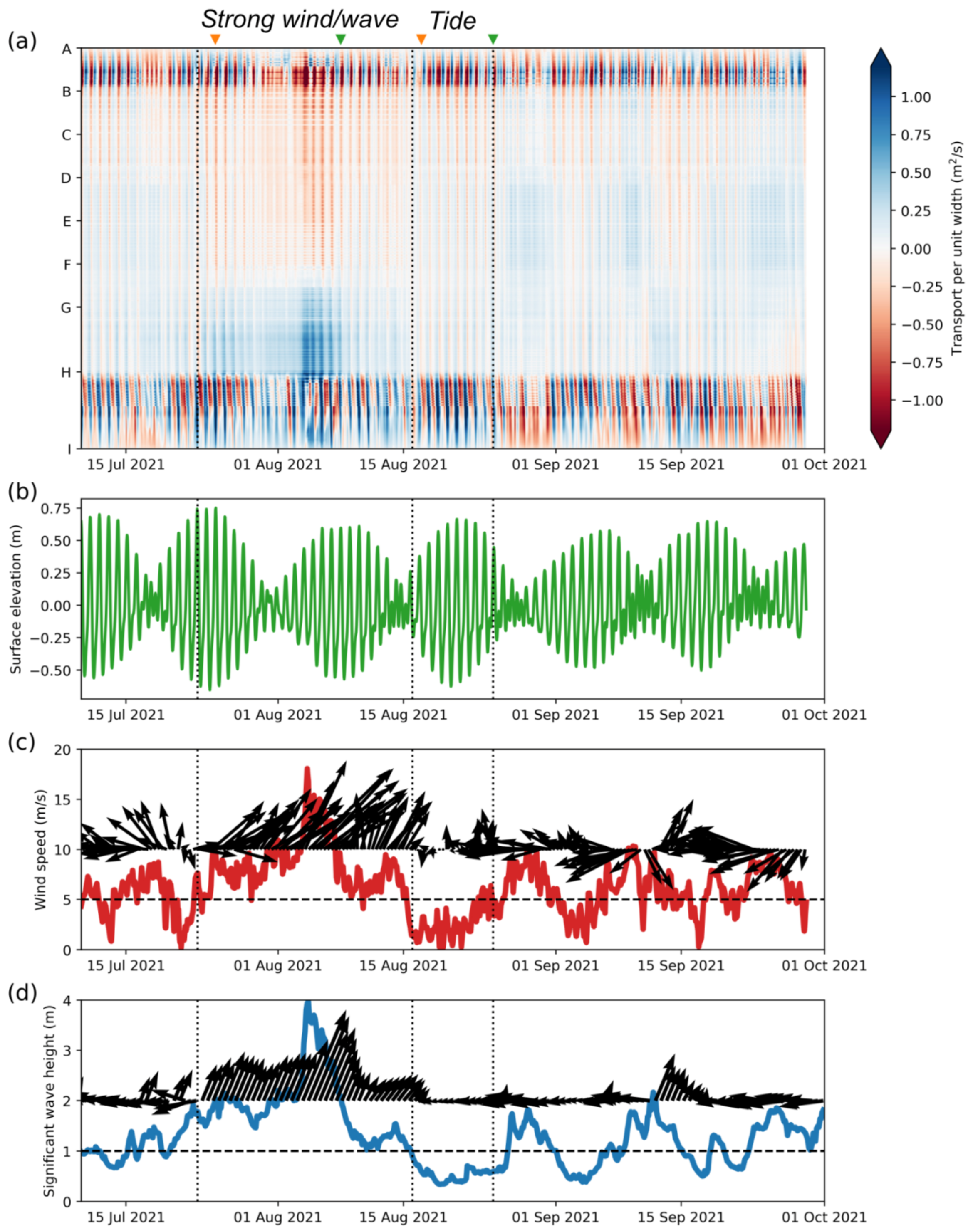
The lagoon water is exchanged with the open ocean water across the lagoon edge (see A to I in Figure 1c). In the northern, eastern, and southern portions of the lagoon edge, the reef flats are submerged below shallow water (about 1 m) and present as barriers. In the west, the north and south channels provide wide (5–10 km) and deep (about 8 m) passages connecting the lagoon and the open ocean. To calculate the transport per unit width across the lagoon edge, a curve connecting locations from A to I (Figure 1c) was discretized, and the water depth was multiplied by the depth-averaged velocity across the curve at each discretized position. The time evolution of transport per unit width across the lagoon edge is shown in Figure 4a. The channels (A to B and H to I in Figure 4a) exhibited higher transports than the reef flat because the channels were deeper than the reef flat. Tidal switches of inflows and outflows were significant (Figure 4a,b). Instead of regular tidal variations, the transport pattern exhibited enhanced outflows at the northern reef flat (B to F) and enhanced inflows at the southern reef flat (F to H) during 23 July and 16 August, as indicated by the first two vertical dotted lines in Figure 4a. Moreover, moderately enhanced inflows at the reef flat appeared around 18 July, 27 August, 10 September, and 27 September, as indicated by the blue patches in Figure 4a.
The characteristics of enhanced transports at the reef flat corresponded to the strengthened wind and waves. During the period from 23 July to 16 August, which is marked as “Strong wave/wave” in Figure 4a, the southwestern wind increased by 18 on 4 August and then decreased by 2 on 16 August (Figure 4c). Meanwhile, the waves from the southwest exhibited an increase of significant wave height by 4 m on 4 August and then a decrease by 1 m on 16 August (Figure 4d). The events of moderately enhanced inflows at the reef flat on around 18 July, 27 August, 10 September, and 27 September also corresponded to a strengthened eastern wind of about 10 and significant wave height of approximately 2 m. However, during a period showing a relatively regular tidally switching pattern of the transport, the wind and waves were relatively weak, such that tides were the dominant forcing (marked as “tide” in Figure 4a).
From a physical perspective, wind stresses drag the sea surface water and lead to along-wind currents. This effect is more obvious in the shallow water than in the deep water because the penetration of wind stresses is limited to the sea surface. As a result, the increasing wind leads to strengthening of the reef flat currents along the wind directions. Waves act in a non-intuitive way. Approaching the fore reef from the open ocean, the incident waves break at a shallow water depth (depth-induced breaking), causing water setup which provides pressure gradient to push water across the reef flat into the lagoon [4,5,6,7,8]. According to this theory, the waves induce strengthened currents at the reef flat facing the incident waves.
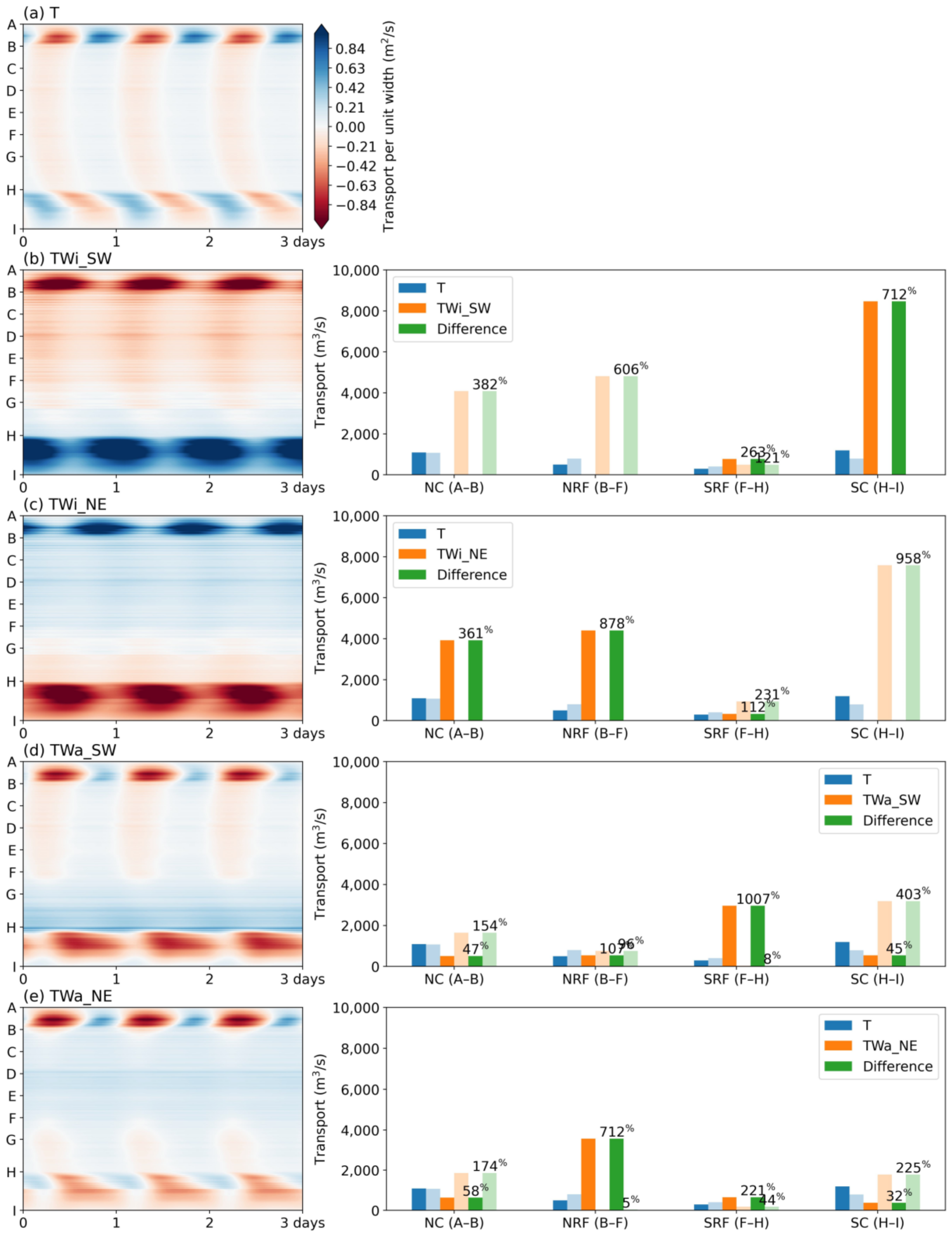
The numerical experiments with simplified and idealized setup of driving forces provide a clear picture for the effects of wind and waves. The left panels of Figure 5 show the time evolution of the transport per unit width along the lagoon edge of the five numerical experiments. The right panels separately show the inflow and outflow transports integrated over different sections of the lagoon edge: the north channel (A–B), the northern reef flat (B–F), the southern reef flat (F–H), and the south channel (H–I). The inflow and outflow transports of the right panels were obtained by temporally averaging the transport per unit width shown in the left panels of Figure 5 but with inflow (positive) and outflow (negative) in different groups, and then the mean inflow and outflow transports per unit width along the lagoon edge were spatially integrated over the four different sections to obtain the inflow transport and outflow transport shown in the right panels of Figure 5. Since I was curious about the amount of additional transport induced by wind and wave forcings, the transport differences between the wind/wave forcing experiments and the baseline experiment T were also calculated (the green bars in Figure 5). The transport differences were calculated by firstly subtracting the transports per unit width at each computational cell along the lagoon edge of experiment T from those of the other experiments, and then the aforementioned calculations of inflow/outflow transports were carried out.
In the baseline experiment T, the transport across the lagoon edge exhibited a regular switch pattern of inflows and outflows due to tides (Figure 5a). The water flew in and out repeatedly at every location of the lagoon edge. The tidal flows at north channel, south channel, and reef flat were asynchronous; water along the lagoon edge did not flow into or out of the lagoon simultaneously. This was probably due to the fact that the tidal waves came from the east; thus, the tidal phases at different locations of the Dongsha Atoll were not the same. A detailed study of this feature is beyond the scope of this manuscript and is left for future work. In the experiment TWi_SW, which represents the typical summer monsoon in this area, the effects of southwestern wind were superimposed on the regular tidal pattern (Figure 5b). The south channel (H–I) and southern reef flat (F–H) exhibited great increases in inflows compared to the experiment T (717% and 263% of the experiment T inflow transports, respectively), and the north channel (A–B) and northern reef flat (B–F) exhibited great increases of outflows (382% and 606% of the experiment T outflow transports, respectively). On the contrary, the experiment TWi_NE suggested that northeastern wind (the winter monsoon) enhanced outflow transports at the south channel and the southern reef flat, and enhanced inflow transports at the north channel and the northern reef flat. The influences of the southwestern and northeastern winds were opposite. Since wind stresses over the sea surface drag water to form the currents along the wind directions, the southwestern wind enhanced transports into the lagoon through the southwestern atoll. On the other hand, it enhanced transports out of the lagoon through the northeastern atoll occur along with the southwestern wind. The reversed directions of the wind-influenced transports occurred for the northeastern wind. It is tricky to determine whether inflow or outflow transports were enhanced at the north channel by the two principal monsoon wind directions because the cross-section orientation of the north channel was roughly southwest–northeast. Instead of being directly influenced by the wind, the transports at the north channel were considered as the compensation for the excess transports through the south channel and the reef flat.
The effects of waves are illustrated by the experiment TWa_SW and TWa_NE, denoting the waves corresponding to the summer and winter monsoon, respectively. The waves coming from the southwest mainly contributed to the inflow transport at the southern reef flat, which was 1007% of the experiment T inflow transport (Figure 5d). This contribution was due to that the incident waves from the open ocean break at the forereef, and the resulting wave setup produced pressure gradient favoring inflow transports. To compensate for the excess inflow transport, the excess outflow transports increased primarily at the south channel (403% of the outflow transport of experiment T) and secondarily at the north channel (96%). The incident waves coming from the northeast, corresponding to the winter monsoon, contributed to the excess inflow transport at the northern reef flat (712%) and the consequent outflow transport at the south channel (225%) and the north channel (174%). This analysis suggests that the effects of waves took place on inflow transports at the reef flat. Whether the waves came from the southwest or the northeast, the wave forcing resulted in excess outflow transports at the two channels.
In Figure 6, the instantaneous surface elevation distributions of the experiments T, TWa_SW, and TWa_NE are shown to illustrate the wave-induced transports. With the tide forcing only, the reef flat all exhibited inflows in the flooding phase and outflows in the ebbing phase (Figure 6a). When the incident waves from the open ocean broke at the fore reef, wave setup was generated at the reef flat, shown by the red patches at the reef flats in Figure 6b,c. The incident directions of the waves determined where the wave setup occurred at the reef flats. The waves from the southeast induced wave setup at the southern reef flat (Figure 6b) and those from the northeast induced wave setup at the northern and eastern reef flat (Figure 6c). This wave setup provided pressure gradient favoring inflows across the reef flat. The enhanced wave-induced reef flat inflows led to enhanced channel outflows. For example, the outflows at the south channel were enhanced because of the enhanced inflows at the southern reef flat (Figure 6a,b). Furthermore, the wave-induced inflows at the southern reef flat seemed to correlate with the outflows at the south channel more than the wave-induced inflows at the north/eastern reef flat did. For example, the resulting south channel outflow transports were greater in TWa_SW than those in TWa_NE (see the flow vectors in Figure 6b,c and the outflow differences at H–I in Figure 5d (403%) and 5e (225%)). Proximity of the south channel and the southern reef flat may be attributed to the tight correlation between the wave-induced southern inflows and the south channel outflows.
Returning to the realistic scenario, the inflow and outflow transports integrated over the north channel, the northern reef flat, the southern reef flat, and the south channel are shown in Figure 7. In order to distinguish the effects by wind/waves and tides, the transports were calculated separately in two periods, 23 July–16 August (strong southwestern wind and waves) and 16 August–25 August (wind and waves were calm; tides dominated). The transport pattern in the tide-dominated period was similar to the baseline experiment T, in that switching of inflows and outflows were relatively homogeneous over the reef flat (Figure 4a and Figure 5a). As the wind and waves effects were introduced to the system during 23 July–16 August, the tidal pattern was superimposed by the intensified outflow transports at the northern reef flat and inflow transports at the southern reef flat, which was consistent with the experiments TWi_SW and TWa_SW. The southwestern wind and waves also intensified the outflow transports at the north channel. At the south channel, the inflow and outflow transports in the tide-dominant and wind–wave-dominated periods were similar. Wind and waves did not seem to modify the flow pattern at the south channel. The reason may be that, according to the experiments TWi_SW and TWa_SW, the former exhibited an intensified inflow transport at the south channel, and the latter exhibited an intensified outflow transport. Thus, the inflow and outflow transports compensated for each other, such that the south channel transports in the two periods in Figure 7 are similar.
Climate statistics were carried out to show the occurrence frequencies of the conditions similar to the wind–wave-dominated period and the tide-dominated period in the aforementioned period of interest. During the wind–wave-dominated period, southwestern wind speeds exceeded 5 and significant wave heights exceeded 1 m. In contrast, the wind speeds were less than 5 and significant wave heights were less than 1 m during the tide-dominated period (see Figure 4c,d). Figure 8 shows statistics of the historical daily data of ERA5 during the period 1959 to 2021. The data location was 117 E, 20.7 N, about 10 km east of the Dongsha. In the entire temporal span, 26.7% of the wind speeds were less than 5 , while this proportion was 38.1% in July, August, and September (JAS) (Figure 8a,c). For waves, 24.8% of the wave heights were less than 1 m in the entire data, while this proportion was 34.5% in JAS. On the basis of these statistics, the tide-dominated condition occurred more in JAS, probably due to relatively calm weather conditions in the summer. By adding the constraint of southwestern incident direction, the occurrence of wind speeds exceeding 5 was 8.3% of the entire data and 19.6% of the data in JAS. For the southwestern waves of more than 1 m, the occurrence was 2.1% of the entire data and 6.2% in JAS. As a result, the occurrence of the southwestern wind–wave-dominated conditions as shown in the period of interest was relatively rare in the region of Dongsha.
4. Discussion
4.1. Hydrodynamic Time Scales to Measure Exchange Rates
In atoll systems, the water properties in the lagoon are different from those in the surrounding seas because the reef flats inhibit water exchange. The degree of the obstruction of reef flats and hydrodynamic processes in the system is related to the exchange rate. Thus, several hydrodynamic timescales have been proposed to measure the exchange rate [44,45,46]. I adopted four of them to measure the different exchange rates during the two regimes, the wind–wave-dominated condition and the tide-dominated condition.
A most intuitive timescale is how much time it takes for the whole volume of the waterbody to be totally renewed by the inflow or outflow water transports. The so-called flushing time is the lagoon volume divided by the inflow transport. Since the inflow transport exhibits tidal variation (Figure 9), the mean value of 7568 was used to divide the lagoon volume (). Thus, the flushing time of the system was about 4.7 days.
The e-folding flushing time is a bulk parameter describing the time needed for a concentration of a material dissolved in a control volume to decay by a factor of exponential [44,46]. It assumes that the control volume is well mixed throughout the domain, and that the exchange between the control volume and the surrounding waters makes the material concentration exhibit exponential decay.
where is the material concentration, is the concentration at time , and is the e-folding flushing time. In this trend, the material concentration decreases to about 37% of the initial concentration after an e-folding flushing time.
To calculate the e-folding flushing time, I numerically released tracers with the initial concentration of 1 throughout the water body of the control volume, which was enclosed by the closed curve from A to H shown in Figure 1c. The maps of depth-averaged concentrations are shown in Figure 10. The tracers were released separately in the period of the wind–wave-dominated condition (25 July; Figure 10a) and tide-dominated condition (17 August; Figure 10b) to distinguish the effects of wind/waves and tides. Under the strong wind and waves, the tracer released on 25 July diffused more quickly than that released on 17 August (Figure 10). After 16 days of releasing, there were no concentrations higher than 37% () in the lagoon for the tracer released in the wind–wave-dominated period, but there were concentrations higher than 37% in the lagoon for the tracer released in the tide-dominated period. This suggests that the wind and waves had greater capability to drive the water exchange. The mechanisms of wind and waves driving water exchange were demonstrated in the numerical experiments in the previous section. By integrating the material concentrations over the whole lagoon volume, the time series of the total material volume of the two tracers are shown in Figure 11. The concentrations decreased approximately according to exponential decay; thus, the e-folding flushing time in Equation (3) was estimated by fitting the exponential decay to the time series of total material volume. The fitting suggests that the system driven by the wind–wave-dominated condition has a shorter e-folding flushing time (4.5 days) than the system driven by the tide-dominated condition (13.4 days). The e-folding flushing time represents a timescale for intercomparisons, i.e., for comparing the flushing rate in different sea conditions or different study sites. It can reveal a general timescale of the flushing rate, but it does not practically state how long the materials, for example, pollutants, nutrients, or dissolved chemicals, in the lagoon take to be expelled. To directly estimate the time which materials take to travel within the lagoon, methods of the Lagrangian perspective are required.
From the Lagrangian perspective, numerical floats were released in the lagoon and tracked to build maps of the residence time and age. The residence time is the time that a water parcel resides in an aquatic system before leaving, and the age is the time that an outside water parcel takes after entering the system [44,45,46]. A schematic plot is shown in Figure 12. They are highly spatially dependent because the distance of each water parcel position from the system boundaries varies. I used a Python package, Parcels, to track passive numerical floats [47] (http://www.oceanparcels.org; accessed on 5 October 2022). It is a framework for computing Lagrangian particle trajectories aiming to be able to process large-scale data generated by contemporary and future ocean general circulation models. The passive numerical floats were evenly released with a spacing of about 200 m in the lagoon (the gray dots in Figure 12) and moved horizontally by the depth-averaged horizontal velocity of the model output. For calculating the residence time , the trajectory of each float was forward tracked (e.g., the blue trajectory in Figure 12). The time it took to leave the lagoon edge was denoted as the residence time of the water parcel at the releasing position (e.g., the black dot in Figure 12). Three releases of floats were carried out in the wind–wave-dominated period (00:00, 01:00, and 02:00 on 25 July; see the orange triangles in Figure 4a) and the tide-dominated period (00:00, 01:00, and 02:00 on 17 August), and the floats were forward tracked in the next 30 days. The residence times of the three releases on 25 July and 17 August were averaged to build the maps of residence time shown in Figure 13a,b, respectively. For calculating the age , the trajectories were backward tracked (e.g., the red trajectory in Figure 12) from the releasing position to acquire the elapsed time after the float entered the lagoon edge. Furthermore, three releases of floats were carried out in the wind–wave-dominated period (00:00, 01:00, and 02:00 on 8 August; see the green triangles in Figure 4a) and the tide-dominated period (00:00, 01:00, and 02:00 25 on August), and the floats were backward tracked in the previous 30 days. The maps of age are shown in Figure 13c,d.
The residence times of the floats released in the wind–wave-dominated period (Figure 13a) were less than 2 days for most of the lagoon edge area. Rapid expelling of the water near the boundary was expected. However, larger residence times of up to 15 days appeared near the southwestern reef flat and the middle lagoon. This distribution of residence times was due to the directions of wind and waves. Figure 14a shows the trajectories corresponding to the floats of residence times larger than 10 days. The floats released near the southwestern reef flat traveled northward, circulated at the northern lagoon, and left the lagoon through the north channel and the northern reef flat. What drove this circulation pattern is that the prevailing southwestern wind and waves during this period drove water entering the lagoon through the southwestern reef flat, according to the process shown in the aforementioned numerical experiments. The southwestern reef flat was an entrance of the water entering the lagoon. The water at the entrance entered and circulated in the lagoon, such that it took more time to leave the lagoon. The south channel was also a potential entrance under the prevailing southwestern wind and waves. However, the wave-driven inflows over the southwestern reef flat squeezed the lagoon water out through the south channel (e.g., a typical pattern shown in the lower panel of Figure 6b), leading to the short residence time at the south channel. On the other hand, the residence time became larger in the absence of strong wind and waves (Figure 13b), in that there was a large area exhibiting a residence time longer than 25 days. The trajectories (Figure 14b) indicate that the floats of residence time longer than 25 days circulated around the whole lagoon and left through the south channel, the north channel, and the northern reef flat. The comparison between Figure 13a,b suggests that the lagoon water left the lagoon more quickly (shorter residence time) under the influence of wind and waves.
The capability of wind and waves to drive water exchange was also reflected by the spatial distributions of the age. The northern lagoon exhibited an age less than 12 days for release in the wind–wave-dominated period, while a large area corresponding to an age >12 days was exhibited for release in the tide-dominated period (Figure 13c,d). The long-age area at the northern lagoon in Figure 13c corresponds to the floats entering the lagoon through the southern reef flat and then moving northward (Figure 14c), which is the circulation pattern due to the southwestern wind and waves. The long-age area at the northern lagoon in Figure 13d also corresponds to the north-moving floats (Figure 14d), presumably caused by the low southern wind around 25 August. The maps of the residence time and age suggest more vigorous water exchange during the wind–wave-dominated period than during the tide-dominated period.
4.2. Diffusion of Pollutants from the Dongsha Island
The aforementioned modeling results suggest that wind and waves provide more persistent driving forces superimposing on the oscillatory tidal forcing. The oscillatory behavior of tides restricts the capability to drive water long distances. For a scenario of pollutants expelled into the lagoon from the human-inhabited Dongsha Island, the polluted water is presumably diluted or relocated more efficiently on the days of strong wind and waves than the days of calm wind and waves. To confirm this statement, I carried out simulations with passive tracers, which act like temperature or salinity but do not interact with the fluid dynamics, to mimic diffusion processes of the polluted water.
The scenario is that the pollutants are expelled from the Dongsha Island to the nearby coastal water in the east, north, west, and south. I released the passive tracers with a concentration of 1 in the full water column within the four circular-shaped (2 km radius) areas (Figure 15a; called the eastern tracer (blue), the southern tracer (orange), the western tracer (green), and the northern tracer (red)). To observe the different diffusion behaviors between the tracers influenced dominantly by wind/waves and those influenced mainly by tides, the tracers were released separately on 25 July, during which strong wind () and wavs () dominated, and 17 August, during which calm wind () and waves () appeared that tidal forcing dominated (see the orange triangles in Figure 4a).
Under the influence of strong wind and waves, the concentrated regions of the tracers were quickly relocated. The paths of diffusion presumably corresponded to the prevailing southwestern wind during this period. After 2 days of strong wind/waves, the eastern tracer diffused toward the northern reef flat, and the concentrated region relocated to the northern reef flat (Figure 15b,c). The southern tracer diffused toward the north channel with the concentrated region near its original location. The western and northern tracers diffused to the northern and eastern coastal regions outside the atoll with a larger degree of diffusion than the eastern and southern tracers. On the other hand, the tides alone did not greatly relocate the concentrated region (Figure 15d,e). The concentrated regions were still close to the original releasing locations. This analysis again depicts the capabilities of wind and waves to drive the water body in the Dongsha Atoll.
5. Conclusions
The pattern of water exchange at the Dongsha Atoll under the influences of tides, wind, and waves was investigated by numerical modeling. The analyses suggest that the southwestern wind could enhance the inflows at the southern reef flat and the outflows at the northern reef flat/north channel. The northeastern wind induced an inverse pattern, in that the enhanced inflows occurred at the north channel/northern reef flat and the enhanced outflows occurred at the south channel. Unlike the wind, the waves always strengthened the inflows at the reef flat, the locations of which depended on the incident directions of the waves, e.g., the waves from the southwestern enhanced inflow transports at the southwestern reef flat. For compensation, the outflow transports at the two channels were enhanced.
By analyzing the hydrodynamic timescales in a wind–wave-dominated period and a tide-dominated period in the realistic modeling, it was suggested that the wind and waves induced more vigorous water exchange because they induced shorter hydrodynamic timescales. The inherent characteristics of spatial dependence of the residence time and age revealed that the directions of wind and waves significantly affected the distributions of residence time and age. This implies that the hydrodynamic processes in the Dongsha Atoll would have significant seasonal variability due to the monsoons in this region. It is worth conducting long-term realistic modeling to investigate the seasonal or even decadal variabilities of this system.
Funding
This research was funded by Taiwan’s National Science and Technology Council, grant numbers MOST 109-2119-M-001-011- and MOST 110-2119-M-001-007-.
Institutional Review Board Statement
Not applicable.
Data Availability Statement
The data that support the findings of this study are available from the corresponding author upon reasonable request.
Acknowledgments
The author thanks Chienhsun Chen for coordinating and conducting the field campaign at the Dongsha Atoll. Shih-Nan Chen, Wu-Ting Tsai, and Yi-Chia Hsin are also gratefully acknowledged for discussions of this topic. The simulations were carried out on the HPC at Taiwan Ocean Research Institute.
Conflicts of Interest
The author declares no conflict of interest.
Appendix A
The governing equations of ROMS in Cartesian horizontal coordinates ( and , assigned to east and north, respectively), sigma vertical coordinate (), and temporal coordinate () are
with the continuity equation
and the scalar transport equation
Here, and are horizontal velocities in and , respectively, is vertical velocity in the vertical sigma coordinate , is free-surface elevation, is a vertical stretching factor due to the terrain-following coordinate, is the Coriolis parameter, is pressure, and are total and background densities, is gravitational acceleration, and are horizontal viscosity and diffusivity, and C denotes tracers (temperature, salt, and passive tracers). Reynold stresses and and turbulent tracer flux are parameterized as
where is vertical velocity in the non-stretched vertical coordinate , and calculations of eddy viscosity and eddy diffusivity rely on turbulent closure schemes (GLS in this study).
The governing equations of SWAN in Cartesian coordinates are reflected by the spectral action balance equation,
where is the action density, is the wave frequency, is the wave direction, and , , , and are wave propagation velocities in , , , and space, respectively. on the right-hand side represents sources and sinks of wave energies.
References
- von Arx, W.S. The circulation systems of Bikini and Rongelap lagoons. Trans. Am. Geophys. Union 1948, 29, 861–870. [Google Scholar] [CrossRef]
- Dufour, P.; Andréfouët, S.; Charpy, L.; Garcia, N. Atoll morphometry controls lagoon nutrient regime. Limnol. Oceanogr. 2001, 46, 456–461. [Google Scholar] [CrossRef]
- Monismith, S.G. Hydrodynamics of Coral Reefs. Annu. Rev. Fluid Mech. 2007, 39, 37–55. [Google Scholar] [CrossRef]
- Symonds, G.; Black, K.P.; Young, I.R. Wave-driven flow over shallow reefs. J. Geophys. Res. 1995, 100, 2639–2648. [Google Scholar] [CrossRef] [Green Version]
- Hearn, C.J. Wave-breaking hydrodynamics within coral reef systems and the effect of changing relative sea level. J. Geophys. Res. Ocean. 1999, 104, 30007–30019. [Google Scholar] [CrossRef]
- Gourlay, M.R.; Colleter, G. Wave-generated flow on coral reefs—An analysis for two-dimensional horizontal reef-tops with steep faces. Coast. Eng. 2005, 52, 353–387. [Google Scholar] [CrossRef]
- Lowe, R.J.; Falter, J.L.; Monismith, S.G.; Atkinson, M.J. Wave-Driven Circulation of a Coastal Reef–Lagoon System. J. Phys. Oceanogr. 2009, 39, 873–893. [Google Scholar] [CrossRef]
- Callaghan, D.P.; Nielsen, P.; Cartwright, N.; Gourlay, M.R.; Baldock, T.E. Atoll lagoon flushing forced by waves. Coast. Eng. 2006, 53, 691–704. [Google Scholar] [CrossRef]
- Dumas, F.; Le Gendre, R.; Thomas, Y.; Andréfouët, S. Tidal flushing and wind driven circulation of Ahe atoll lagoon (Tuamotu Archipelago, French Polynesia) from in situ observations and numerical modelling. Mar. Pollut. Bull. 2012, 65, 425–440. [Google Scholar] [CrossRef]
- Taebi, S.; Lowe, R.J.; Pattiaratchi, C.B.; Ivey, G.N.; Symonds, G.; Brinkman, R. Nearshore circulation in a tropical fringing reef system. J. Geophys. Res. 2011, 116, C02016. [Google Scholar] [CrossRef]
- Becker, J.M.; Merrifield, M.A.; Ford, M. Water level effects on breaking wave setup for Pacific Island fringing reefs: Water level effects on wave setup. J. Geophys. Res. Ocean. 2014, 119, 914–932. [Google Scholar] [CrossRef]
- Costa, M.B.; Macedo, E.C.; Valle-Levinson, A.; Siegle, E. Wave and tidal flushing in a near-equatorial mesotidal atoll. Coral Reefs 2017, 36, 277–291. [Google Scholar] [CrossRef]
- Atkinson, M.; Smith, S.V.; Stroup, E.D. Circulation in Enewetak Atoll lagoon1: Enewetak circulation. Limnol. Oceanogr. 1981, 26, 1074–1083. [Google Scholar] [CrossRef]
- Tartinville, B.; Deleersnijder, E.; Rancher, J. The water residence time in the Mururoa atoll lagoon: Sensitivity analysis of a three-dimensional model. Coral Reefs 1997, 16, 193–203. [Google Scholar] [CrossRef] [Green Version]
- Douillet, P.; Ouillon, S.; Cordier, E. A numerical model for fine suspended sediment transport in the southwest lagoon of New Caledonia. Coral Reefs 2001, 20, 361–372. [Google Scholar] [CrossRef]
- Mathieu, P.-P.; Deleersnijder, E.; Cushman-Roisin, B.; Beckers, J.-M.; Bolding, K. The role of topography in small well-mixed bays, with application to the lagoon of Mururoa. Cont. Shelf Res. 2002, 22, 1379–1395. [Google Scholar] [CrossRef]
- Lowe, R.J.; Falter, J.L.; Monismith, S.G.; Atkinson, M.J. A numerical study of circulation in a coastal reef-lagoon system. J. Geophys. Res. 2009, 114, C06022. [Google Scholar] [CrossRef] [Green Version]
- Lentz, S.J.; Davis, K.A.; Churchill, J.H.; DeCarlo, T.M. Coral Reef Drag Coefficients—Water Depth Dependence. J. Phys. Oceanogr. 2017, 47, 1061–1075. [Google Scholar] [CrossRef] [Green Version]
- Wang, Y.-H.; Dai, C.-F.; Chen, Y.-Y. Physical and ecological processes of internal waves on an isolated reef ecosystem in the South China Sea. Geophys. Res. Lett. 2007, 34, L18609. [Google Scholar] [CrossRef]
- Chen, G.-Y.; Wu, R.-J.; Wang, Y.-H. Interaction between internal solitary waves and an isolated atoll in the Northern South China Sea. Ocean Dyn. 2010, 60, 1285–1292. [Google Scholar] [CrossRef]
- Fu, K.-H.; Wang, Y.-H.; Laurent, L.S.; Simmons, H.; Wang, D.-P. Shoaling of large-amplitude nonlinear internal waves at Dongsha Atoll in the northern South China Sea. Cont. Shelf Res. 2012, 37, 1–7. [Google Scholar] [CrossRef] [Green Version]
- Reid, E.C.; DeCarlo, T.M.; Cohen, A.L.; Wong, G.T.F.; Lentz, S.J.; Safaie, A.; Hall, A.; Davis, K.A. Internal waves influence the thermal and nutrient environment on a shallow coral reef. Limnol. Oceanogr. 2019, 64, 1949–1965. [Google Scholar] [CrossRef] [Green Version]
- Davis, K.A.; Arthur, R.S.; Reid, E.C.; Rogers, J.S.; Fringer, O.B.; DeCarlo, T.M.; Cohen, A.L. Fate of Internal Waves on a Shallow Shelf. J. Geophys. Res. Ocean. 2020, 125, e2019JC015377. [Google Scholar] [CrossRef]
- Xu, A.; Chen, X. A Strong Internal Solitary Wave with Extreme Velocity Captured Northeast of Dong-Sha Atoll in the Northern South China Sea. J. Mar. Sci. Eng. 2021, 9, 1277. [Google Scholar] [CrossRef]
- Chen, Y.; Chen, L.; Zhang, H.; Gong, W. Effects of wave-current interaction on the Pearl River Estuary during Typhoon Hato. Estuar. Coast. Shelf Sci. 2019, 228, 106364. [Google Scholar] [CrossRef]
- Prakash, K.R.; Pant, V. On the wave-current interaction during the passage of a tropical cyclone in the Bay of Bengal. Deep Sea Res. Part II Top. Stud. Oceanogr. 2020, 172, 104658. [Google Scholar] [CrossRef]
- Calvino, C.; Dabrowski, T.; Dias, F. A study of the wave effects on the current circulation in Galway Bay, using the numerical model COAWST. Coast. Eng. 2023, 180, 104251. [Google Scholar] [CrossRef]
- Hersbach, H.; Bell, B.; Berrisford, P.; Hirahara, S.; Horanyi, A.; Muñoz-Sabater, J.; Nicolas, J.; Peubey, C.; Radu, R.; Schepers, D.; et al. The ERA5 global reanalysis. Q. J. R. Meteorol. Soc. 2020, 146, 1999–2049. [Google Scholar] [CrossRef]
- Warner, J.C.; Armstrong, B.; He, R.; Zambon, J.B. Development of a Coupled Ocean–Atmosphere–Wave–Sediment Transport (COAWST) Modeling System. Ocean Model. 2010, 35, 230–244. [Google Scholar] [CrossRef] [Green Version]
- Haidvogel, D.B.; Arango, H.G.; Hedstrom, K.; Beckmann, A.; Malanotte-Rizzoli, P.; Shchepetkin, A.F. Model evaluation experiments in the North Atlantic Basin: Simulations in nonlinear terrain-following coordinates. Dyn. Atmos. Ocean. 2000, 32, 239–281. [Google Scholar] [CrossRef]
- Shchepetkin, A.F.; McWilliams, J.C. The regional oceanic modeling system (ROMS): A split-explicit, free-surface, topography-following-coordinate oceanic model. Ocean Model. 2005, 9, 347–404. [Google Scholar] [CrossRef]
- Booij, N.; Ris, R.C.; Holthuijsen, L.H. A third-generation wave model for coastal regions: 1. Model description and validation. J. Geophys. Res. Ocean. 1999, 104, 7649–7666. [Google Scholar] [CrossRef] [Green Version]
- Ris, R.C.; Holthuijsen, L.H.; Booij, N. A third-generation wave model for coastal regions: 2. Verification. J. Geophys. Res. Ocean. 1999, 104, 7667–7681. [Google Scholar] [CrossRef]
- Kumar, N.; Voulgaris, G.; Warner, J.C.; Olabarrieta, M. Implementation of the vortex force formalism in the coupled ocean-atmosphere-wave-sediment transport (COAWST) modeling system for inner shelf and surf zone applications. Ocean Model. 2012, 47, 65–95. [Google Scholar] [CrossRef]
- Amante, C.; Eakins, B.W. ETOPO1 1 Arc-Minute Global Relief Model: Procedures, Data Sources and Analysis; National Geophysical Data Center, NOAA: Boulder, CO, USA, 2009. [Google Scholar] [CrossRef]
- Chapman, D.C. Numerical Treatment of Cross-Shelf Open Boundaries in a Barotropic Coastal Ocean Model. J. Phys. Oceanogr. 1985, 15, 1060–1075. [Google Scholar] [CrossRef]
- Flather, R.A. A tidal model of the northwest European continental shelf. Mem. Soc. R. Des Sci. De Liege 1976, 6, 141–164. [Google Scholar]
- Egbert, G.D.; Erofeeva, S.Y. Efficient Inverse Modeling of Barotropic Ocean Tides. J. Atmos. Ocean. Technol. 2002, 19, 183–204. [Google Scholar] [CrossRef]
- Fairall, C.W.; Bradley, E.F.; Hare, J.E.; Grachev, A.A.; Edson, J.B. Bulk Parameterization of Air–Sea Fluxes: Updates and Verification for the COARE Algorithm. J. Clim. 2003, 16, 571–591. [Google Scholar] [CrossRef]
- Rogers, J.S.; Monismith, S.G.; Fringer, O.B.; Koweek, D.A.; Dunbar, R.B. A coupled wave-hydrodynamic model of an atoll with high friction: Mechanisms for flow, connectivity, and ecological implications. Ocean Model. 2017, 110, 66–82. [Google Scholar] [CrossRef] [Green Version]
- Komen, G.J.; Hasselmann, K.; Hasselmann, K. On the Existence of a Fully Developed Wind-Sea Spectrum. J. Phys. Oceanogr. 1984, 14, 1271–1285. [Google Scholar] [CrossRef]
- Madsen, O.S.; Poon, Y.-K.; Graber, H.C. Spectral Wave Attenuation by Bottom Friction: Theory. In Proceedings of the 21st Conference on Coastal Engineering, Torremolinos, Spain, 20–25 June 1988; Volume 1, p. 34. [Google Scholar] [CrossRef]
- Willmott, C.J. On the validation of models. Phys. Geogr. 1981, 2, 184–194. [Google Scholar] [CrossRef]
- Monsen, N.E.; Cloern, J.E.; Lucas, L.V.; Monismith, S.G. A comment on the use of flushing time, residence time, and age as transport time scales. Limnol. Oceanogr. 2002, 47, 1545–1553. [Google Scholar] [CrossRef] [Green Version]
- Rayson, M.D.; Gross, E.S.; Hetland, R.D.; Fringer, O.B. Time scales in Galveston Bay: An unsteady estuary. J. Geophys. Res. Ocean. 2016, 121, 2268–2285. [Google Scholar] [CrossRef] [Green Version]
- Jouon, A.; Douillet, P.; Ouillon, S.; Fraunié, P. Calculations of hydrodynamic time parameters in a semi-opened coastal zone using a 3D hydrodynamic model. Cont. Shelf Res. 2006, 26, 1395–1415. [Google Scholar] [CrossRef]
- Delandmeter, P.; van Sebille, E. The Parcels v2.0 Lagrangian framework: New field interpolation schemes. Geosci. Model Dev. 2019, 12, 3571–3584. [Google Scholar] [CrossRef]
Figure 1.
(a) A map showing the location of the Dongsha Atoll and (b) the modeling domain used in this study. The morphology of the Dongsha Atoll, including Dongsha Island, the north channel, the south channel, and the reef flat, is indicated in (b). The black lines represent a 1 m isobath to indicate the reef flat and the Dongsha Island. (c) A zoomed-in view showing the two measurement sites (H10 and N09) and the location indicators (A–I).

Figure 2.
(a) Wind speed (red) and direction (arrows), (b) significant wave height, (c) net surface heat flux, and (d) net surface freshwater flux during the period of interest. Panels (a,c,d) were derived from ERA5, and panel (b) was derived from the MFWAM performed by Météo-France.
Figure 2.
(a) Wind speed (red) and direction (arrows), (b) significant wave height, (c) net surface heat flux, and (d) net surface freshwater flux during the period of interest. Panels (a,c,d) were derived from ERA5, and panel (b) was derived from the MFWAM performed by Météo-France.

Figure 3.
Comparisons of the modeled results against the observations at (a) site H10 and (b) site N09. From top to bottom: surface elevation, eastward depth-averaged velocity, northward depth-averaged velocity, significant wave height, and peak wave period.
Figure 3.
Comparisons of the modeled results against the observations at (a) site H10 and (b) site N09. From top to bottom: surface elevation, eastward depth-averaged velocity, northward depth-averaged velocity, significant wave height, and peak wave period.

Figure 4.
(a) Transport per unit width at the edge of Dongsha Atoll lagoon. Positive (negative) values represent the flows into (out of) the lagoon. The vertical axis denotes the same location indicators as shown in Figure 1c, and the horizontal axis is time. The dashed lines indicate a wind–wave-dominated and a tide-dominated (weak wind and waves) period. The two orange triangles (25 July and 17 August) and two green triangles (8 August and 25 August) show the times of releasing tracers (see Section 4 for details). (b) Surface elevations showing spring and neap tides. (c) Wind speed (red) and wind vectors (arrows). (d) Significant wave height (blue) and wave vectors (arrows).

Figure 5.
Left panels: time evolutions of transport per unit width along the lagoon edge of the experiments. Right panels: Inflow transports (heavy color) and outflow transports (pale color) integrated over the north channel (A–B), the northern reef flat (B–F), the southern reef flat (F–H), and the south channel (H–I). The blue bars denote the baseline experiment T, and they appear in each panel for comparison. The orange bars denote the additional wind/wave forcing experiments. The green bars are transport differences of the additional wind/wave forcing experiments from the baseline experiment T, representing additional transports induced by wind or wave forcings. The amounts of the difference are also expressed as percentages of the experiment T transport, which are labeled on top of the green bars.

Figure 6.
Instantaneous surface elevation distributions of the experiments. The top panels are in the phase of flooding, and the bottom panels are in the phase of ebbing.
Figure 6.
Instantaneous surface elevation distributions of the experiments. The top panels are in the phase of flooding, and the bottom panels are in the phase of ebbing.

Figure 7.
Inflow transports (heavy color) and outflow transports (pale color) integrated over the north channel (A–B), the northern reef flat (B–F), the southern reef flat (F–H), and the south channel (H–I). Blue (orange) bars represent mean transports during the period of 16 August to 25 August (23 July–16 August).

Figure 8.
Histograms of (a,c) wind speed and (b,d) significant wave height (combined wind waves and swells) during the period 1959 to 2021 (data source: ERA5, daily). Panels (a,b) were derived from the entire data, and panels (c,d) were derived from the data in July, August, and September (JAS). The lines denote accumulation percentages.

Figure 9.
Total transport (gray), inflow transport (blue), and outflow transport (red) integrated over the lagoon edge (A–I). The inflow and outflow transports were calculated by integrating the positive and negative transports separately.
Figure 9.
Total transport (gray), inflow transport (blue), and outflow transport (red) integrated over the lagoon edge (A–I). The inflow and outflow transports were calculated by integrating the positive and negative transports separately.

Figure 10.
Depth-averaged concentrations over time (from left to right). They were released on (a) 25 July, in the wind–wave-dominated period, and (b) 17 August, in the tide-dominated period. The gray contours indicate 37% () and 1% of the initially released concentration.
Figure 10.
Depth-averaged concentrations over time (from left to right). They were released on (a) 25 July, in the wind–wave-dominated period, and (b) 17 August, in the tide-dominated period. The gray contours indicate 37% () and 1% of the initially released concentration.

Figure 11.
Time evolutions of the total material volume in the lagoon, shown as percentages of the initial total material volume (blue: released on 25 July 2021; orange: released on 17 August 2021). The gray lines are exponential functions of least squares fitting of the two timeseries.
Figure 11.
Time evolutions of the total material volume in the lagoon, shown as percentages of the initial total material volume (blue: released on 25 July 2021; orange: released on 17 August 2021). The gray lines are exponential functions of least squares fitting of the two timeseries.

Figure 12.
A schematic plot which illustrates the concept of residence time () and age ( ). Taking a water parcel at the black dot as an example (the arrows indicate traveling directions), it comes from the open ocean in the path of the red curve and goes outside the lagoon in the path of the blue curve. Therefore, age is the duration of the path marked by , and residence time is the duration of the path marked by . The gray dots represent the passive numerical floats released for calculating residence time and age.

Figure 13.
Spatial distributions of the residence time calculated with the forward tracking floats released on (a) 25 July and (b) 17 August (see the orange triangles in Figure 4a) and age calculated with the backward tracking floats released on (c) 8 August and (d) 25 August (see the green triangles in Figure 4a).

Figure 14.
Trajectories of the high-residence-time floats which were (a) released on 25 July ( days) and (b) released on 17 August ( days), and high-age floats which were backward tracked from (c) 8 August ( days) and (d) 25 August ( days). In (a,b), the black dots indicate the initial positions of the trajectories, while, in (c,d), the black dots indicate the final positions of the trajectories.

Figure 15.
Distributions of the passive tracers released in the realistic model. (a) Initial releasing position (25 July and 17 August). (b,c) Depth-averaged concentrations of the tracers (released on 25 July) on 26 July and 27 July, respectively; (d,e) depth-averaged concentrations of the tracers (released on 17 August) on 18 August and 19 August, respectively. The gray contours in (b–e) indicate 1% of the initial concentration.


Table 1.
Summary of the numerical experiments.
| Label | Tides | Wind | Waves |
|---|---|---|---|
| T | K1 | n/a | n/a |
| TWi_SW | K1 | SW | n/a |
| TWi_NE | K1 | NE | n/a |
| TWa_SW | K1 | n/a | SW |
| TWa_NE | K1 | n/a | NE |
The wind and wave forcings all correspond to the wind speed of about 14
Table 2.
Skill scores (SS), Pearson correlation coefficients (), root-mean-square error (RMSE), and bias of model outputs against observations.
Table 2.
Skill scores (SS), Pearson correlation coefficients (), root-mean-square error (RMSE), and bias of model outputs against observations.
| SS | RMSE | Bias | |||
|---|---|---|---|---|---|
| H10 | Surface elevation | 0.995 | 0.99 | 0.033 | −0.011 |
| Eastward depth-averaged velocity | 0.8 | 0.73 | 0.029 | −0.011 | |
| Northward depth-averaged velocity | 0.79 | 0.73 | 0.032 | 0.012 | |
| Significant wave height | 0.88 | 0.78 | 0.099 | 0.021 | |
| Peak wave period | 0.50 | 0.39 | 4.612 | 3.706 | |
| N09 | Surface elevation | 0.99 | 0.996 | 0.035 | −0.014 |
| Eastward depth-averaged velocity | 0.53 | 0.40 | 0.011 | −0.002 | |
| Northward depth-averaged velocity | 0.60 | 0.38 | 0.019 | −0.002 | |
| Significant wave height | 0.58 | 0.41 | 0.107 | 0.060 | |
| Peak wave period | 0.44 | 0.24 | 4.314 | 3.343 |
Disclaimer/Publisher’s Note: The statements, opinions and data contained in all publications are solely those of the individual author(s) and contributor(s) and not of MDPI and/or the editor(s). MDPI and/or the editor(s) disclaim responsibility for any injury to people or property resulting from any ideas, methods, instructions or products referred to in the content. |
© 2023 by the author. Licensee MDPI, Basel, Switzerland. This article is an open access article distributed under the terms and conditions of the Creative Commons Attribution (CC BY) license (https://creativecommons.org/licenses/by/4.0/).
Share and Cite
MDPI and ACS Style
Chen, S.-M. Water Exchange Due to Wind and Waves in a Monsoon Prevailing Tropical Atoll. J. Mar. Sci. Eng. 2023, 11, 109. https://doi.org/10.3390/jmse11010109
AMA Style
Chen S-M. Water Exchange Due to Wind and Waves in a Monsoon Prevailing Tropical Atoll. Journal of Marine Science and Engineering. 2023; 11(1):109. https://doi.org/10.3390/jmse11010109
Chicago/Turabian StyleChen, Shi-Ming. 2023. "Water Exchange Due to Wind and Waves in a Monsoon Prevailing Tropical Atoll" Journal of Marine Science and Engineering 11, no. 1: 109. https://doi.org/10.3390/jmse11010109
Note that from the first issue of 2016, this journal uses article numbers instead of page numbers. See further details here.