A Robust and Efficient Computational Fluid Dynamics Approach for the Prediction of Horizontal-Axis Wind Turbine Performance

Abstract

In spite of the tremendous advances in computing power and continuous improvements in simulation software made in recent decades, the accurate estimation of wind turbine performance using numerical methods remains challenging. Wind turbine aerodynamics, especially when operating outside of the design envelope, is highly complex: blade stall, laminar-to-turbulent boundary layer transition, rotational effects (lift augmentation near blade root), and tip losses are present. The scope of this research is to show that the classic Reynolds-Averaged Navier–Stokes (RANS) modeling approach, although extensively tried and tested, is not yet exhausted. The NREL Phase VI rotor was used as a basis for numerical methodology development, verification and validation. The numerical model results are compared in detail with the available measured data, both globally (turbine torque and thrust, and blade bending moment) and locally (pressure coefficient distributions and aerodynamic force coefficients at several locations on the blade) over the entire experimental wind speed range. Stall initiation and spread over the blade span are well captured by the model, and rotor performance is predicted with good accuracy. RANS still presents significant value for wind turbine engineering, with a great balance between accuracy and computational cost. The present work brings potential impact on all applications of wind turbines, especially targeting offshore wind energy extraction for which great development is expected in the near future.

1. Introduction

Wind turbines, in general, might appear as relatively simple devices and be regarded as sufficiently well understood from an engineering point of view. However, their aerodynamic behavior is rather complex and significantly more sophisticated than usually considered. This complexity raises proportionally large difficulties that need to be overcome in order to be able to predict their performance with a high degree of accuracy and to improve their efficiency using computational methods. Moreover, just as with many other engineering applications, including more physics in the wind turbine modeling, in an attempt to improve the fidelity of the numerical results, this easily leads to a disproportionate increase in the associated computational effort. Consequently, the aim of the present work was to find a way to obtain results with sufficient accuracy for engineering purposes, which is generally applicable and does not necessarily incur high costs in terms of computational time or power.

Within the current context for the energy sector and the European Union targets for drastically reducing greenhouse gas emissions, the Marine Renewable Energy solution is being paid increased attention. A 25-fold growth in the 2021 offshore wind energy extraction capacity alone is projected for 2050. Taking into account these figures, it is obvious that any efforts that can improve the accuracy vs. computational cost ratio are valuable. At the same time, technological advances in the current design of offshore wind turbines, in general, can hardly be made without reliable and robust methods that can help engineers to confidently and efficiently test and validate design changes or new ideas.

Blade Element Momentum (BEM) theory was, and continues to be, widely used for wind turbines basic aerodynamic analysis, structural loads and stability analysis, and control design [1]. This is a natural consequence of the low computational requirements of BEM models and acceptable accuracy potential at operating regimes where the underlying assumptions of the method are valid. In practice though, turbine designers need to run procedures which involve multiple iterative loops, and the computational efficiency becomes decisive, often pushing the use of BEM out of its confidence domain.

Computational Fluid Dynamics (CFD) is a very capable, well-proven and generally applicable method that can be used for the numerical modeling and simulation of all types of wind turbines. Its greatest disadvantage is, in comparison with BEM, the necessary computing power; however, during the last decade or so, the availability of relatively cheap and easy to access clustered computing machines drastically shortened the turnaround time. Consequently, CFD is nowadays a perfectly viable alternative, even for routine calculations. The source of its computational requirements is, obviously, its mathematical formulation, which is also its greatest strength, since—at least in theory—it makes CFD truly predictive and applicable to any design or operating regime. Traditionally, CFD formulation is based on the Navier–Stokes (N-S) model of fluid flow, but other approaches do exist, such as the Lattice–Boltzmann method (LBM). Being inherently unsteady, the LBM is computationally very demanding; nevertheless, as most of the high-level applications related to wind turbines (e.g., yawed operation) involve strongly unsteady flows, it can be regarded as a good candidate, particularly in the context of GPU computing. The works of Pérot et al. [2], Dieterding and Wood [3], Schottenhamml et al. [4], and Xue et al. [5] demonstrate the use of the LBM for simulation of isolated turbines, including hub and tower, or multiple turbines with wake interaction, and even large-scale wind farm flow simulations, with simplified modeling of turbines by coupling actuator line models with the LBM. Given the aim of this research, we do consider that the LBM does not fit our goal and should be reserved for purposes where large-scale, high temporal and spatial resolution is mandatory.

The classic, N-S model-based CFD approach offers several well-established possibilities: (a) the steady-state Reynolds-Averaged N-S (RANS) modeling of isolated blades in moving reference frames using periodic boundaries is, by far, the most affordable and most frequently used (the majority of the reviewed papers are based on this approach), (b) the unsteady RANS is sometimes used, but only if the added cost is justified, for example when the relative motion and interaction between the rotor and the tower needs to be taken into consideration, in conjunction with moving grids (deforming/rebuilding or overset) (for example, the work of Bangga et al. [6], who investigated various configurations of vertical-axis wind turbines, for which this approach is practically unavoidable) and (c) hybrid RANS-LES modeling, when unsteady effects are dominant, not just close to the turbine blades, but also downwind, e.g., flow separation and wake interaction(an example is the work of Sorensen and Schreck [7], discussed below). The computational cost increases exponentially from (a) to (c) and, as far as the overall turbine performance is concerned, steady-state RANS still strikes the best balance between computational effort and output value for engineering activities. Another possibility is the bi-directional coupling between an unsteady CFD model and a computational structural dynamics model to simulate the aero-elastic response of the rotor blades; but that is also very costly and difficult to handle.

The NREL Phase VI Unsteady Aerodynamic Experiment (UAE) [8] provides an excellent starting point for testing and validating CFD software and/or methodologies. The introduction of the UAE data set to the research community after completion of testing in May 2000 consisted of a blind test prediction using a very diverse range of performance, aero-elastic, wake, and CFD codes (19 distinct modeling tools, in total). The blind comparison study was implemented in such way as to identify uncertainties associated with wind turbine model predictions that included the effects of both the modeling tool and methodology used. Results from the report [9] published by NREL at the end of the blind test analysis clearly indicate that, globally, the comparison was not favorable: wide variations between various codes, significant deviations from measured wind tunnel data, and unacceptable scatter under typical turbine operating conditions were revealed. For example, under no-yaw, steady-state, no-stall conditions, turbine power predictions ranged from 25% to 175% of measured, and blade bending-force predictions ranged from 85% to 150% of measured. Results at higher wind speeds, under stall conditions, were especially disappointing, considering that power predictions ranged from 30% to 275% of measured and blade-bending predictions ranged from 60% to 125% of measured. The results from the two N-S CFD codes included in the blind test, although far from being perfect, were much more consistent overall, demonstrating good predictive potential (at least from a qualitative point of view) and dependable modeling practices.

Following the blind test, many researchers have investigated the NREL Phase VI configuration numerically using a variety of CFD methods and grid topologies. One of the notable early works is the analysis performed by Sorensen et al. [10] published in 2002. The paper actually also contains the results that were submitted to the NREL blind test two years before, and consist of the six S-series required cases. Computations were run with the EllipSys3D code on two different multi-block structured grids, one representing a so-called free configuration (pre-test) and the other a tunnel configuration (post-test). Grid sizes were relatively small (3.1 M cells and 4.2 M cells, respectively), severely limited by the available computational resources. The SST k-omega model of Menter was used for turbulence modeling. Deviation of computed integrated loads from experimental data was significant, with 20% over-prediction of stall onset (10 m/s case) shaft torque, and similar under-prediction of deep-stall torque. One very important aspect was the observation that the tunnel configuration, although overall not much better than the free configuration, does bring a little bit of improvement for the 10 m/s wind speed case, with some weak separation of flow near the r/R = 0.47 section of the blade.

In 2003, Benjanirat et al. [11] used an academic 3D unsteady Navier–Stokes solver to test several turbulence models: the Baldwin–Lomax Model, the Spalart–Allmaras one-equation model, and the k-ε two-equation model with and without wall corrections. Normal forces and associated bending moments were calculated with decent accuracy, but chordwise forces, rotor torque and pitching moments estimations were unacceptable, markedly so between 10 and 20 m/s wind speed.

The same year, Duque et al. [12] performed Navier–Stokes simulations on the NREL Phase VI rotor using the Overflow-D2 code, developed by NASA, and compared the results with the rotorcraft comprehensive commercial code Camrad II, which used various stall delay and dynamic stall models. A structured overset grid system was used to represent both blades, without nacelle and tower, totaling 11.5 M nodes. Computations were performed for both axial as well as yawed operating conditions. The Navier–Stokes computations were shown to more accurately predict stalled rotor performance and also revealed significant spanwise flow. Although the N-S-model-calculated normal force coefficient indicates a good agreement with the experimental data at r/R = 0.47 and 10 m/s wind speed, the corresponding pressure coefficient plot reveals an attached local flow distribution.

In 2004, Le Pape and Lecanu [13] used ONERA’s structured multi-block solver elsA, to model the NREL UAE in an upwind, zero-yaw configuration. The single-blade model had two variants, with and without blade root; both meshes were the same size, just under 1 M cells. Two variations of the k-omega turbulence model were tested, namely the Wilcox k-omega and the SST k-omega. Their efforts to ensure high mesh quality resulted in torque and thrust predictions that were in good agreement with the experimental data at lower wind speeds, before the onset of stall. However, at moderate speeds, stall was predicted too early, leading to under-prediction of torque. The model without blade root performed consistently worse in all cases.

Rooij and Arens [14] focused on the augmented lift phenomenon as a result of blade rotation in the steady-state, non-yawed condition, in 2007. They applied the commercial Fluent code for the simulation of the UAE conditions, concentrating on the cases between 8 and 15 m/s wind speed, in steps of 1 m/s. Steady-state solutions using the SST k-omega model were obtained, unsteady calculations with the same model and DES computations were run on a multi-block structured 3.6 M cells mesh, representing an isolated blade in a spherical, large domain. The SST k-omega model results proved more reliable, and to the surprise of the authors, there was little difference between steady and unsteady results. The predictions are quite good in general, for all blade sections and normal force coefficient analysis proves that the inboard segments at r/R = 0.30 and r/R = 0.47 experience augmented lift and stall delay as a consequence of rotation; however, their calculations completely fail to reproduce the initiation of blade stall approximately 10 m/s wind speed.

The NSU3D unstructured commercial code was used by Potsdam and Mavriplis [15] to simulate the behavior of NREL Phase VI rotor. Steady-state and time-accurate calculations were run on a range of meshes with different topologies and also adaptive mesh refinement was investigated with the intention to better capture the turbine wake; the resulting meshes grew significantly, close to 40 M cells (compared to 6 M for the overset structured mesh). They found that performance results obtained with the unstructured code compare favorably with those obtained with the structured overset solver Overflow, but concluded that the unstructured meshing approach may require more nodes for the same level of accuracy. In the end neither of the attempted methodologies was able to correctly predict stall at 10 m/s, while the estimated thrust and torque were very inconsistent between models.

A study by Yu et al. [16] published in 2010 presents the results obtained with an (unspecified) incompressible RANS solver for the NREL Phase VI configuration based on UAE conditions, for wind speeds between 5 and 10 m/s. Again, a multi-block structured mesh was used, though relatively small, with only 2.9 M cells; y+ approximately 1 and a low expansion ratio are provided. Steady-state CFD solution results are presented, employing the SST k-omega model. Pressure coefficient plots for 10 m/s wind speed show a fully separated flow condition at r/R = 0.47 section and a reasonably good match with the experimental data, except r/R = 0.63 section where predicted separation is excessive. Pre-stall numerical results are very good, locally and globally; most importantly though, stall inception is properly captured.

Lanzafame et al. [17] introduced in their 2012 work the four-equation Transitional SST k-omega model and compared it to the classic two-equation SST turbulence model. The ANSYS Fluent solver was used, while the meshing strategy was based on an unstructured hybrid method, with prismatic boundary layers and polyhedral volume-filling cells. The empirical correlations of the Transitional SST turbulence model were modified by performing a significant number of numerical 2D airfoil tests prior to the 3D calculations. Model validation was concluded by comparison with UAE data for rotor power. Remarkably good match of measured power was claimed, up to 18 m/s wind speed—actually, the most favorable comparison to date, according to our knowledge—with the modified Transitional SST model. The alternatively presented two-equation SST k-omega model results are acceptable, apart from the 10 to 14 m/s interval, where they deviate significantly from measurements. No information about the modified transition correlations was given. Pressure coefficient plots or local force and moment coefficients were not included.

Essentially, most of the presented works did not involve disproportionately large efforts in order to achieve a reasonable level of accuracy. This is principally due to the use of steady or unsteady RANS methodologies, with mostly coarse meshes. Attempts to push the accuracy limits associated with such approach did exist; for example, Sorensen and Schreck [7] published their research on DDES with laminar–turbulent transition modeling in 2014. A fully structured 36 M cells mesh was constructed for an isolated rotor model and five wind speeds were tested (between 10 and 20 m/s). Compared to RANS solution obtained with the same model, DDES did not improve power prediction, but predicted the energy contents of the unsteady flow much better than RANS. DDES was able to reproduce the low frequency shedding along the blade, failing to capture the high frequency fluctuations (most likely due to still insufficient mesh resolution).

LES solutions, either wall-modeled or wall-resolved, of the UAE conditions are, most likely, impossible to achieve with the current computing systems due to tremendous near-wall mesh density requirements. Therefore, it seems that practical modeling approaches for medium to large wind turbines that are applicable to engineering activities favor RANS, for now.

Michna et al. [18] verified the Gamma Re-Theta Transition Model by simulating the DU-91-W2-250 airfoil at high Re numbers (between 3 × 10⁶ and 6 × 10⁶) and comparing the results with fully-turbulent models and experimental data. They observed that the error in estimating the location of the transition was significant at the low end of the Re range, decreasing with Re. They concluded that the un-calibrated transition SST approach for a 2D thick airfoil should not be applied beyond the critical angle of attack. Additionally, Rogowski et al. [19] applied the same transitional model to a 2D NACA 0018 airfoil model at a Re number of 1.6 × 10⁶. Their results show significant improvements of the transitional model compared to the two-eq. SST k-omega model, at higher angles of attack. In conclusion, laminar-to-turbulent flow transition modeling has the potential to improve the CFD predictions; however, the current implementations of transitional models are not universally applicable out-of the box and may need tuning to return reliable results, which is not a trivial task.

In the following we intend to show that the classic RANS methods should not be disregarded yet. Adopting careful meshing techniques and making proper physical and numerical modeling choices, improvements on results accuracy can be made, without resorting to models customization or other non-standard procedures. From our experience with the NREL Phase VI rotor modeling, but also corroborating with some of the results presented above, the mesh topology, resolution and distribution might play a much more important role than commonly understood. Generally speaking, the modeling phase is critical for the success of the wind turbine simulation efforts.

2. Methodology

2.1. NREL Phase VI Configuration

The Unsteady Aerodynamic Experiment (UAE, starting 1987) was designed to provide extensive information about the full-scale, 3D aerodynamic phenomena characteristic to the operation of horizontal-axis wind turbines (HAWT). Field testing revealed that these 3D effects are dominant in wind turbine field operation. These tests also showed that the turbulent inflow and shear through the rotor plane resulted in highly dynamic loads. Unfortunately, extracting the 3D operational effects from the field data was not possible, and the need for a controlled, anomaly-free testing environment was identified. Consequently, a complex test campaign (1999) was conducted by the National Renewable Energy Laboratory (NREL) at the National Full-Scale Aerodynamics Complex (NFSAC) wind tunnel, located in NASA Ames Research Center.

In the open-loop configuration, the NFSAC wind tunnel has a 24.4 m (H) × 36.6 m (W) test section, and it is capable of up to 50 m/s flow velocities. The power is provided by six 15-bladed fans, each driven by a 16,800 kW electric motor. Tunnel blockage was estimated to be less than 2% for all conditions encountered during testing, and less than 1% for the majority of cases [9]. Streamwise turbulence levels were typically less than 0.5%; for the lower wind speeds, turbulence levels closer to or even higher than 2% were recorded during the experiment, but these deviations were caused by the measurement system uncertainties at the lower pressure levels [9].

The 10 m diameter, stall-regulated wind turbine used for the wind tunnel testing campaign was a two-bladed configuration, with a power rating of 20 kW. The blades were non-linearly twisted and linearly tapered. Both downwind and upwind configurations were tested. The turbine rotor was mounted on a 12.2 m high tower, such that the rotor axis was on the tunnel centerline. Multi-disciplinary measurements were obtained over a wide range of operating conditions. Experimental measurements included blade pressures and resulting integrated aerodynamic loads, rotor shaft torque, sectional inflow conditions, blade root strain, tip acceleration and wake visualization. Both upwind and downwind configurations with rigid and teetering blades were run for speeds from 5 to 25 m/s. Yawed and unsteady pitch configurations are also available. Free and fixed transition results were measured. The blade was designed and constructed using the highly specialized S809 airfoil for which experimental aerodynamic performance parameters are available [20]. Blade structural properties are well documented [8].

From the total of 1700 experimental data sets available, only a subset of the S-series was selected for the CFD modeling. The S-series measurements were based on an upwind, no probes baseline blade, with rigid setup, no cone angle, no yaw, 3.0 deg blade tip pitch configuration. Every data set between 7 and 12 m/s, and every other data set between 13 and 25 m/s were retained, to a total of 13 cases.

Table 1. Computational cases.

Case ID	Wind Velocity	Air Density	Viscosity 1 (10−5)	Rotor Speed
	[m/s]	[kg/m3]	[Pa·s]	[rpm]
S0700000	7.0163	1.2458	1.7708	71.867
S0800000	8.0499	1.2437	1.7729	71.999
S0900000	9.0133	1.2457	1.7708	72.098
S1000000	10.047	1.2459	1.7700	72.096
S1100000	11.039	1.2285	1.7823	72.099
S1200000	12.057	1.2271	1.7836	72.105
S1300000	13.069	1.2266	1.7834	72.094
S1500000	15.098	1.2240	1.7858	72.062
S1700000	17.115	1.2230	1.7860	72.007
S1900000	19.090	1.2216	1.7870	72.017
S2100000	21.165	1.2209	1.7872	72.043
S2300000	23.207	1.2194	1.7881	72.116
S2500001	25.109	1.2197	1.7868	72.162

¹ Data computed using the three-coefficient Sutherland’s formula.

summarizes the data corresponding to each of the 13 experimental cases.

2.2. Geometric Modeling

The geometric model of the NREL Phase VI blade was created based on the information published in [6]. This document was made available to all the participants of the initial blind testing, and contains very detailed information about all the relevant machine parameters, rotor blade geometry, power train and tower characteristics, aerodynamic and structural properties.

2.2.1. S809 Airfoil

Specifically designed for HAWT applications, the S809 airfoil is a 21-percent-thick, laminar-flow airfoil, with a limited maximum lift coefficient of 1.0, generally intended for small-to-medium turbines to be used on the outboard sections. More information about the design and experimental testing of this airfoil can be found in [20].

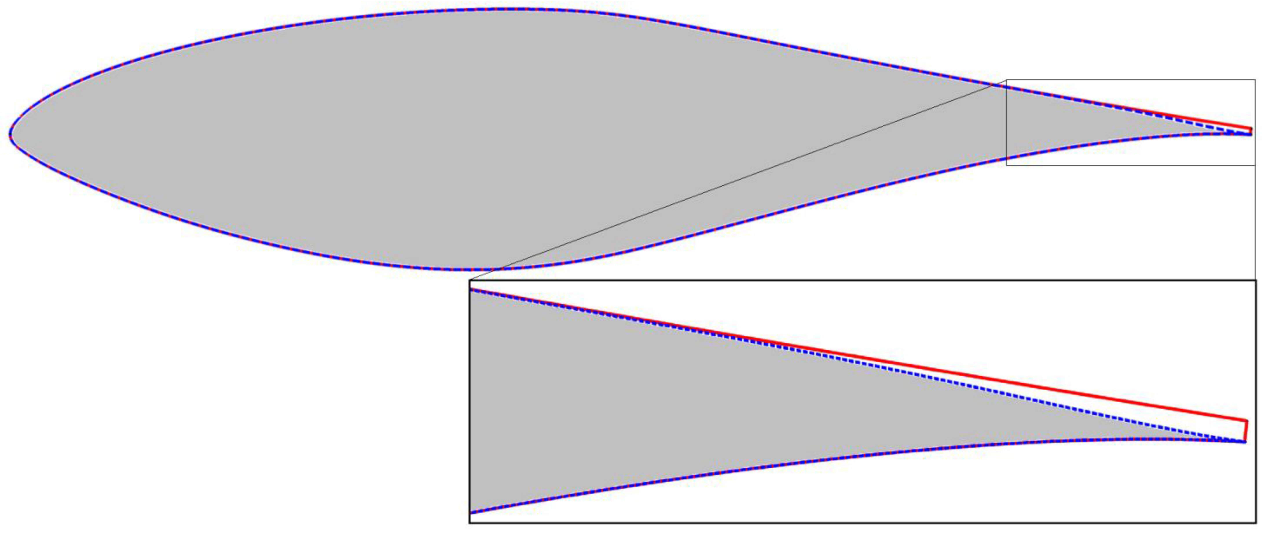
The original S809 airfoil has a sharp trailing edge (TE). This feature is generally acceptable for 2D CFD modeling, using either structured or unstructured meshing methods; however, it is not realistic since the blade cannot be fabricated with such sharp edge due to structural limitations. Additionally, for 3D CFD modeling, it is better to avoid it; not only it unnecessarily complicates the closing of the tip geometry, but also causes many difficulties during the meshing process. Unstructured prismatic layers would include very high angles in the near-wall cells close to the TE, while the structured meshing techniques typically applied for this type of geometry (combinations of O-type and H-type grids) would also generate highly skewed cells in the vicinity of the blade’s TE. Therefore, the original geometry was altered by introducing a blunt TE with a thickness of 0.5% of chord length, through the controlled deformation of the suction curve.

Lee et al. [21] intentionally exaggerated the thickness the TE of NREL Phase VI rotor blade and tried to assess the effects of this modification on turbine performance. The lowest blunting tested (1% of chord length) showed very little variation compared to the baseline (unmodified) blade.

A graphical representation of the airfoil shape alteration result can be examined in Figure 1. One can notice that the original shape of the airfoil suction side exhibits a strange variation near the TE, going from concave to convex and back to concave, which results in a double inflection point. The second concavity, closest to TE, was suppressed by moving the suction side TE point upwards from the original position, (1, 0) in non-dimensional coordinates, to (1, 0.005), splitting the initial B-spline interpolating curve near the foremost inflection point, discarding the aft segment and replacing it with a cubic spline with tangency continuity at the splitting point, which connects the new suction side TE point with the remaining suction side curve. The new suction side is thus free from inflection points near the TE and has a continuous concave shape. Even after making all these changes, the airfoil angle of attack (AOA) was not altered, because the reference point used for angle calculations was kept at the original sharp TE location (now the pressure side end of the blunt TE).

2.2.2. Rotor Blade

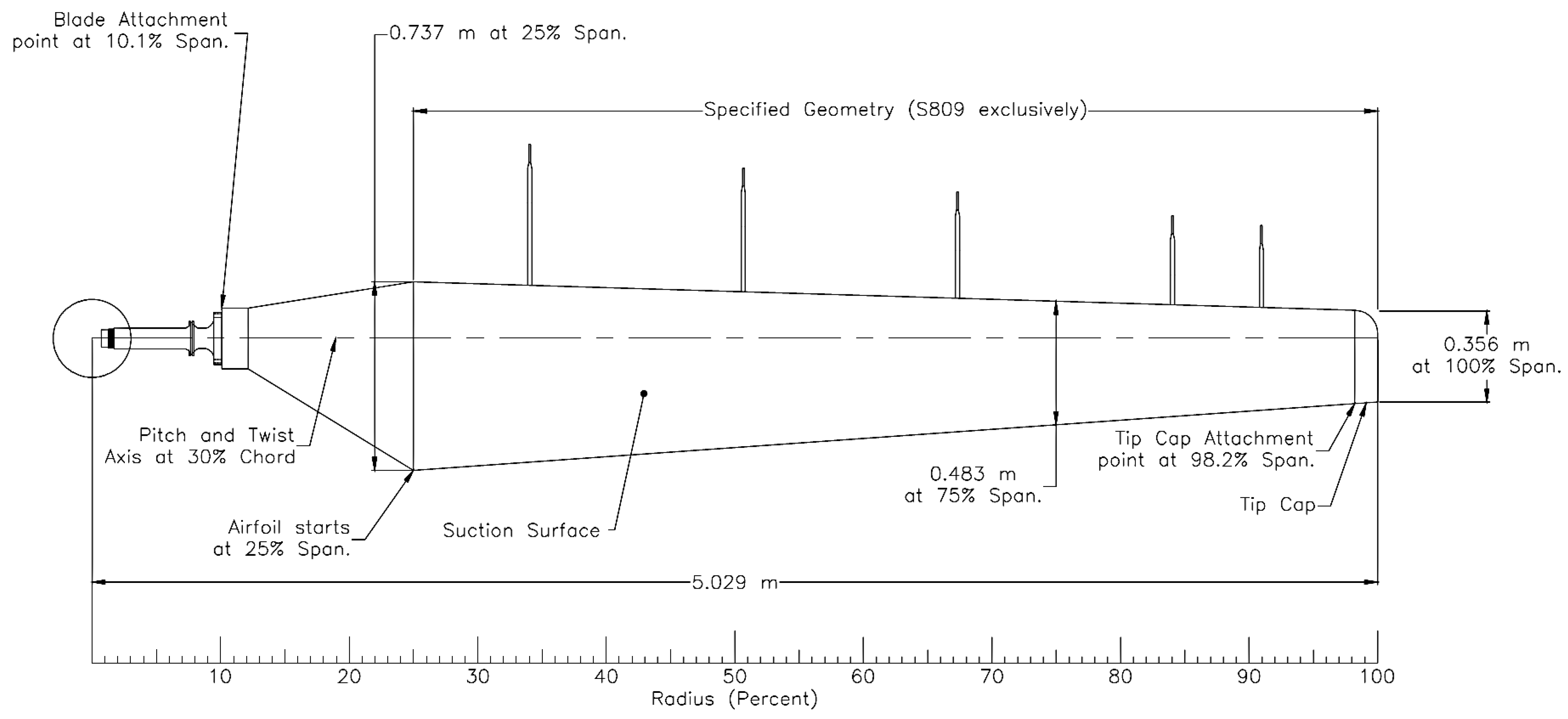
The baseline blade tip radius is 5.029 m. Each of the two blades attaches to the hub section at a radius of 0.508 m from the rotational axis. A cylindrical section extends from 0.508 to 0.883 m, followed by a transition from the circular pitch shaft attachment to the S809 airfoil between 0.883 and 1.257 m. The blade has a linearly variable chord from 0.737 m at the 1.257 m radial location down to approx. 0.356 m at the blade tip. The non-linear twist of the blade is presented in the documentation using the blade section at 75% of rotor radius as reference. This results in slightly more than 20 deg positive twist at the 1.257 m radial station and approx. 1.8 deg negative twist at the blade tip. Care must be exercised when positioning the blade against the global reference coordinate system of the numerical model, because the reference section used for specifying the blade angle during the wind tunnel testing was the blade tip. The blade planform dimensions are presented in Figure 2.

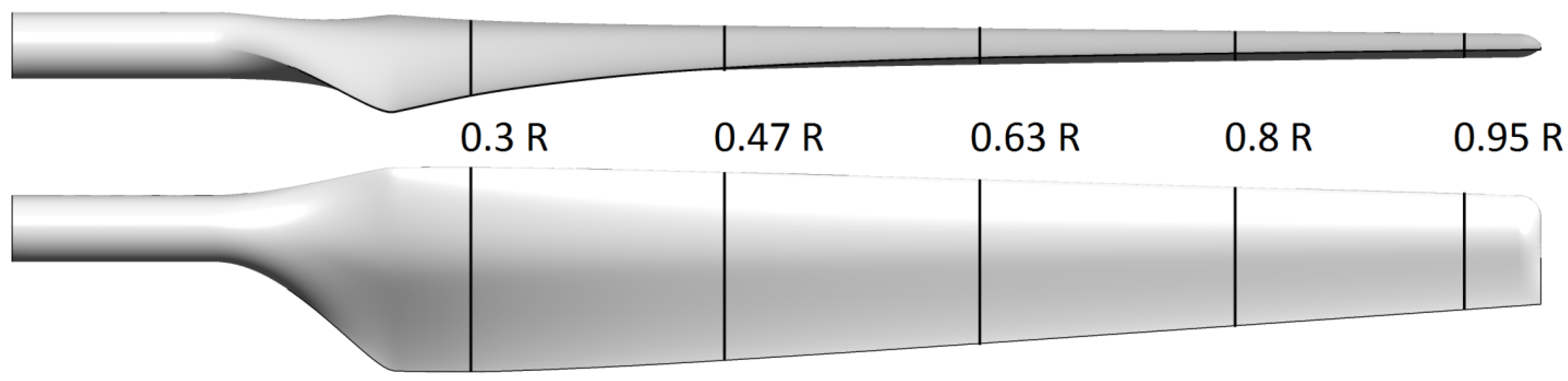
The transition piece geometry is quite coarsely described in the Machine Data file; therefore, a decision was made to simplify this region of the blade by representing it as a smooth transition between the 0.883 m circular section and the 1.257 m radial station airfoil. The corresponding geometric representation was built by imposing tangency continuity at both ends, and also by controlling the interpolating surfaces through tensioned spline curves. No details other than the tip cap attachment point location are given on the blade tip geometry, and only a few images are available. Using the discernible information from these pictures, a tip model was constructed as closely resembling to the real one as possible. The effort was justified by the expected importance of this particular detail to the accuracy of the simulated flow in this region of the blade, which was thought to have a significant impact on the overall numerical model fidelity.

In order to simplify the geometry and consequently the meshing process, the rotor hub was completely eliminated and the 0.508 m circular section was extended down to the symmetry plane. For this particular turbine, this is an arguable simplification, since the instrumentation enclosures placed in front of the rotor plane might play an important role in the flow field structure near the blade root. This effect, combined with the alteration of the transition piece geometry probably contributes to the reduced quality of numerical predictions for pressure distribution at the 30% blade radial section. Nevertheless, the influence of these errors on the global rotor performance prediction is considered to be of little importance, as the aerodynamic forces and moments are much more significant on the outboard section of the blade. Obviously, this assumption holds as long as the rotor yaw is zero or small enough, at higher yaw the forward placed instrumentation would definitely alter the flow field over a certain rotor angular sector and blade span, depending on the yaw angle.

Figure 3 presents the geometrical model of the rotor blade as it was used in the construction of the numerical model. The blade root transition piece and the rounded tip geometry are clearly visible. The positioning of the five radial stations where the pressure taps were installed on the experimental rotor is indicated.

2.3. Computational Domain

Under the assumption that the aerodynamic influences of the boom, instrumentation enclosures, turbine tower and tunnel walls can be neglected, at least for the zero-yaw cases, the geometric and solution periodicity can be used. This means that the numerical model can be reduced to only one blade, while the effects of the other blade are accounted for by using periodicity boundary conditions, effectively reducing the computational effort by 50%. However, a rotationally symmetrical shape must be assumed for the computational domain, the cylindrical domain being the most commonly adopted.

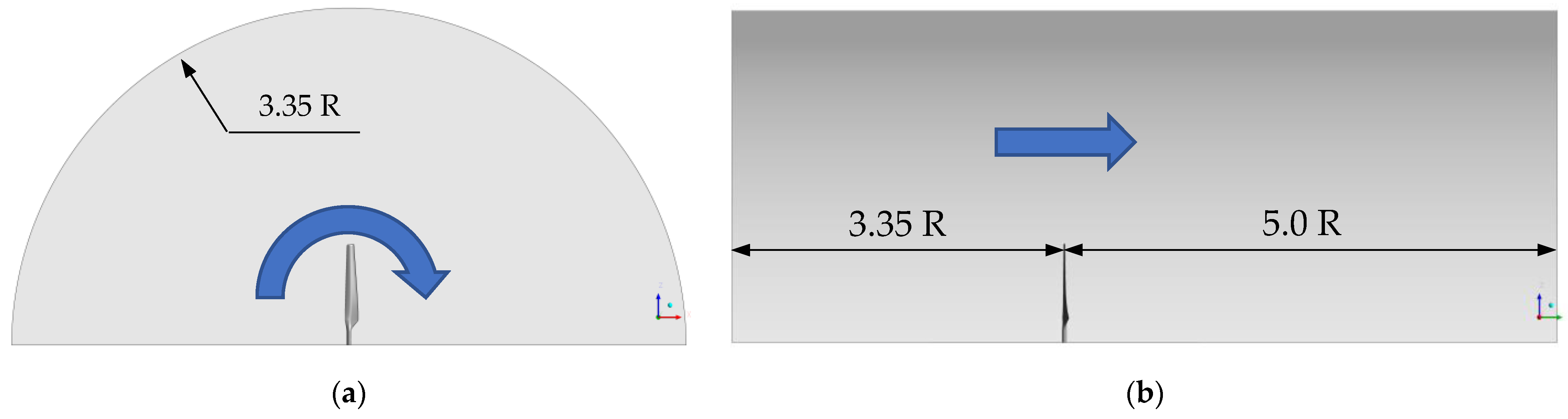
Although Sørensen et al. [10] have concluded that there is very little difference between the results obtained based on a free-rotor assumption, employing a large, very low blockage computational domain, and the results obtained from a wind-tunnel type domain, which restricts the cross-section area of the flow volume to be equal to the actual wind tunnel cross-section area, the latter variant was preferred for the present study. In order to satisfy the equivalence condition, the external radius of the computational domain was limited to 3.35 fold the blade tip radius.

In our previous studies [22], by examining the numerical solution it was concluded that the length of the computational domain in front and behind the rotor plane could be made relatively short without affecting the solution accuracy. Consequently, 3.35 blade lengths in front and 5 blade lengths behind the rotor were considered to be sufficient. Using the 180-degree periodicity condition, the resulting shape of the flow domain presented in Figure 4 is effectively semi-cylindrical.

The ANSYS Fluent CFD solver offers the possibility to simulate rotational boundary flows using either an absolute or a relative reference frame. Considering that the computational domain is rotating as a solid body, the relative reference frame method can be applied to the entire flow domain, but this option is generally not recommendable for wind turbines due to the numerical issues caused by high relative velocities and relative velocity angles near the external boundary. To avoid this problem, a subdivision of the computational domain containing the near-blade region must be created, restricting the rotational motion to this zone only. However, this limits the meshing topologies that can be used and forces unnecessary nodal clustering towards the boundaries, when using structured meshing methods. The advisable alternative that was also applied for the present study is to use the absolute reference frame method, specifying the whole domain as rotating, which allows for much more flexibility regarding the meshing strategy.

2.4. Mesh Design and Construction

In our prior efforts [22], we chose to use a hybrid structured-unstructured meshing approach; a volume within one chord normal distance from the blade was meshed with purely hexahedral multi-block structured grid, the surrounding near-field was filled with tetrahedrons, while the rest of the domain was meshed using prismatic cells. While this method allows for a good control of the mesh nodes density and distribution, the numerical results proved unconvincing. It was concluded that the fully structured meshing approach, although much more laborious and time consuming, might be more appropriate for this particular problem. There have been studies of NREL Phase VI rotor that used unstructured meshing strategies (tetrahedrons and prismatic boundary layer type mesh) testing the feasibility of this meshing topology [15]. However, at least from our point of view, the results were rather unfavorable to the use of unstructured or hybrid meshes; moreover, the vast majority of published results have relied on relatively coarse structured meshes and still obtained quite good results, regardless. Hence, the decision to use fully structured type meshing was taken.

While designing the mesh topology, four conditions have been considered: (a) to attain a high node count on the blade surface, both circumferentially and longitudinally, thus ensuring a good mesh resolution in all directions, not just normal to the blade, (b) to provide sufficient mesh resolution in the wake region, (c) to avoid creating excessively high-aspect-ratio cells, which can be very detrimental to solution stability if stretched too much normal to the flow direction, and (d) to minimize the cell skewness and cell volume ratio. It was decided that the best possible topology that should satisfy to the highest degree all of these conditions simultaneously would be a combination of O-type, C-type and H-type topologies. The O-type grid should envelop the blade completely and smoothly extend from the blade surface mesh radially up to a distance that would not over-disperse the surface nodal density and, at the same time, allow for a low skewness and volume ratio transition to the rest of the mesh. The C-type topology should be applied in the transversal plane to project the mesh radially onto the cylindrical external boundary of the flow domain, while the H-type grid should be used in the longitudinal direction to retain the cross-sectional mesh density, especially behind the blade, with good control over the downstream mesh density and minimal cell deformation.

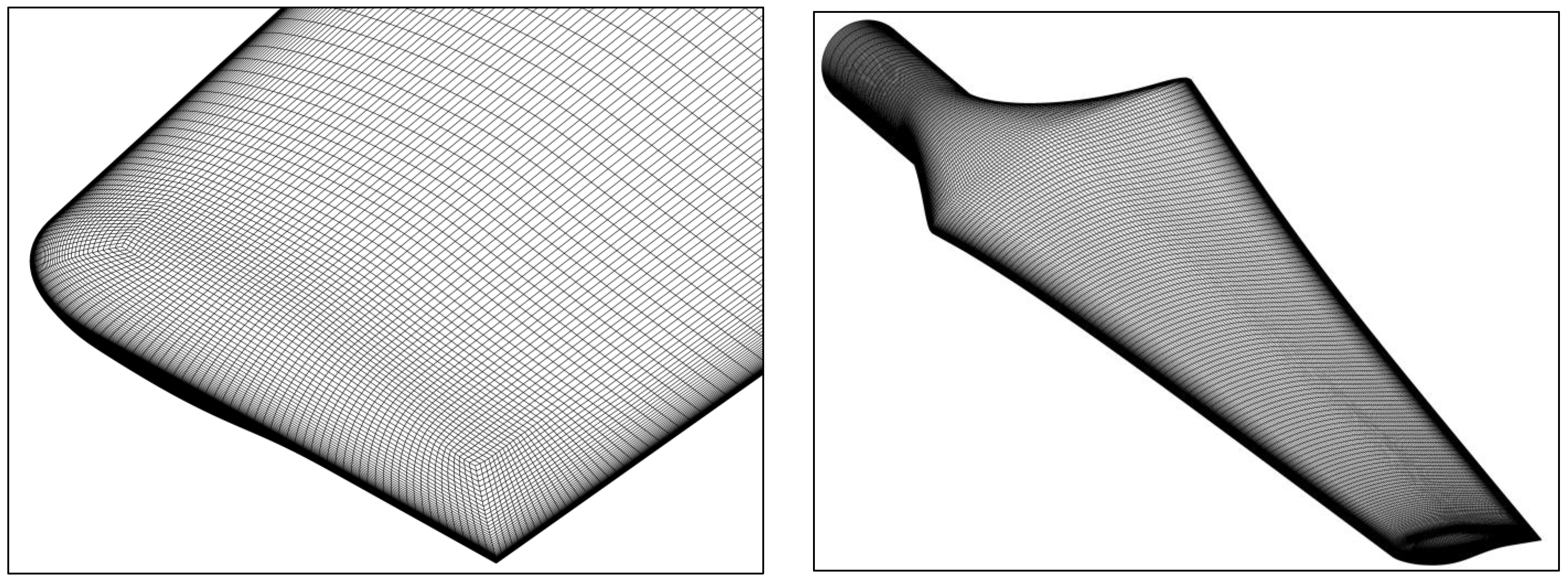
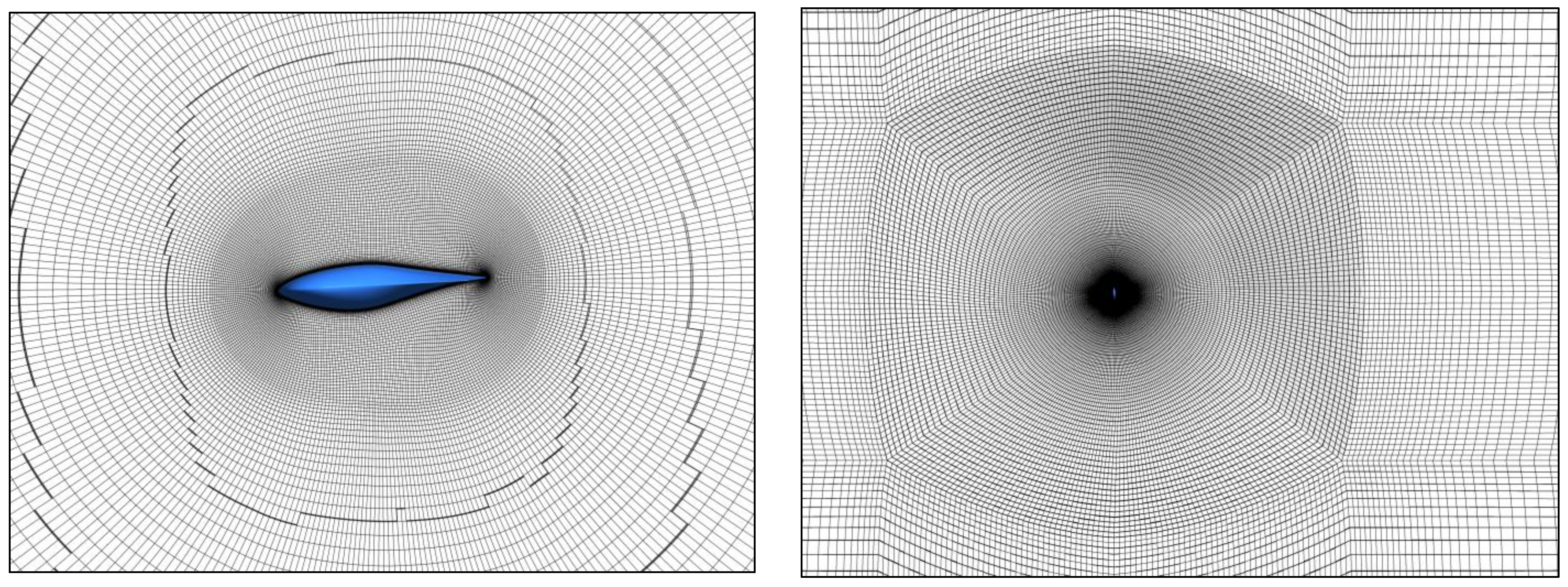
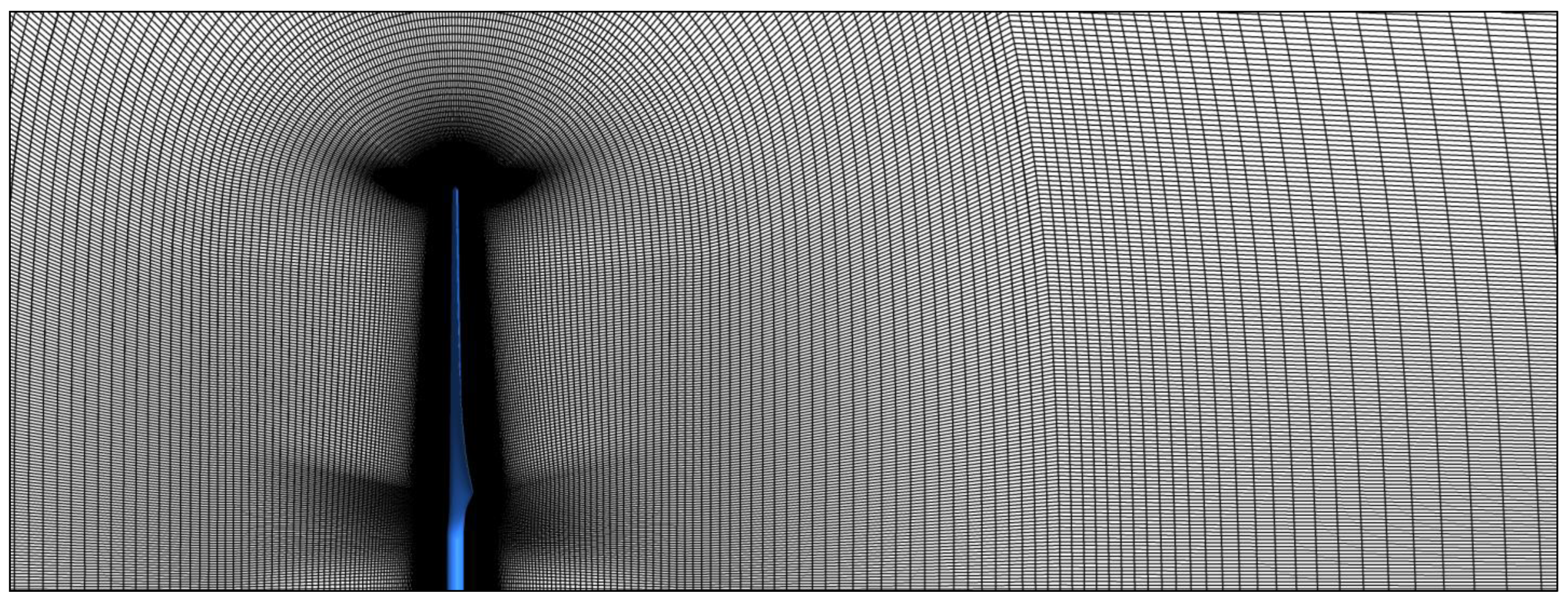
Mesh construction began from the blade surface, which was divided into five blocks: one 60 × 183 on each side, one around the leading edge and one around the trailing edge, size 88 × 183 each, with 8 cells across the blunt TE, plus one 60 × 88 block closing the mesh at the blade tip. The final surface mesh for the blade has almost 59.5 k nodes; as a side note, in order to match the resulting surface mesh nodal distribution and density by using an unstructured topology, a much higher node count would have been required—the high curvature leading edge (which constitutes a large fraction of the total blade surface area) and the thin trailing edge are difficult to cover with nearly-isotropic elements. The blade surface blocks were then swept radially in three successive stages, up to approximately 1.5 blade lengths. The front and back blocks were then projected onto the inlet and outlet surfaces, respectively, resulting in a central mesh core over the entire length of the computational domain, which was then projected onto the outer cylindrical surface. The inner blocks were subsequently divided as required to attain maximum control over the mesh distribution and skewness. The final mesh contains 75 blocks.

In order to correctly simulate the boundary layer flow, the first cell layer height on the blade surface was determined such as to guarantee a y+ value near 1 over the entire blade length. Due to the relative velocity variation along the blade, imposing a y+ close to 1 at the tip and a constant first layer height would generate unnecessarily high normal mesh density towards the blade root. This issue was avoided by constructing several sections through the O-type mesh core first, each section with its own first layer height; the assigned values were approximated using a linear spanwise variation, from 0.012 mm at the blade tip, up to 0.036 mm at the 1.257 m radial station. From there, downwards to the symmetry plane, the normal spacing was maintained constant. This technique improves the radial mesh distribution as well, if the normal growth ratio is the same at all blade sections. Extreme care was taken to enforce and preserve mesh orthogonality and smoothness, both for the surface and volume meshes. The blade normal spacing growth ratio was kept below 1.2 close to the blade surface and much lower than that overall.

The result of the meshing efforts can be examined in Figure 5, Figure 6 and Figure 7. The total cell count is approx. 10.3 M. By design, a significant portion of the mesh is, in fact, contained in the blocks near to the blade surface—3.6 M cells (35% of total) within half a chord (see Figure 6).

Table 2. Mesh quality statistics.

Criteria	Min. Value	Max. Value	Average
Equiangle skewness	-	0.6219	0.1056
Minimum angle	34.03	-	80.60
Aspect ratio	-	2303	34.18
Volume ratio	-	1.596	1.099

summarizes the mesh quality analysis results. The remarkably low equiangle skewness and volume ratio metrics indicate that the final mesh quality is very good overall. It seems that the only criterion which might need improvement is the cell aspect ratio, but all the high-aspect-ratio cells are located near the leading edge (LE) and TE, and the single most efficient way to deal with this issue is to increase spanwise mesh density. Unfortunately, due to the particularities of the chosen meshing structure, this would have a major impact on the total cell count, as the refinement cannot be confined to the near-blade region without using non-conformal interfaces. Nonetheless, the flow in the LE and TE vicinity is mostly two-dimensional, and there is little need to modify the mesh, as long as the boundary layer flow is modeled using RANS approximations.

2.5. Numerical Modeling and Simulation

The commercial software platform ANSYS 14.5 was used for preparing the numerical model, running the calculations and extracting the relevant data. ANSYS Fluent was employed as the CFD solver.

The rotationally periodic boundary condition available in ANSYS Fluent allows the simulation of only one blade under the assumption that the geometry and the flow field are circumferentially periodic and the flow is aligned with the axis of rotation. In order to simulate the rotation, the moving reference frame model was employed. With this model, the equations of motion are modified to incorporate the additional acceleration terms which occur due to the transformation from the stationary to the moving reference frame. By solving these equations in a steady-state or time-dependent manner, the flow around the moving parts can be modeled. The entire flow domain was considered to be rotating with the blade, and an absolute velocity formulation was specified. When the absolute velocity formulation is used, the governing equations are written with respect to the domain’s reference frame, but the velocities are stored in the absolute frame.

The 2D/3D simulations of the S809 airfoil that were performed in the model development phase, the conclusions from our previous work [22] and also the experiences of other researchers, have suggested that the SST k-omega turbulence model (Menter [23]) is a good compromise between accuracy and computational effort. Although generally being insufficiently accurate to be considered a reference for the reliable numerical prediction of aerodynamic drag and lift forces, the SST k-omega is superior to other two-equation turbulence models for external flow simulation. We chose to incorporate the low-Re number modifications that have been proposed by Wilcox for the k-omega model to reproduce the peak in the turbulence kinetic energy observed in DNS data very close to the wall [24]. As a side-effect, these terms affect the laminar–turbulent transition process, by producing a delayed onset of the turbulent wall boundary layer and constitute, therefore, a very simple model for laminar–turbulent transition. Since this property was most probably not necessarily the intent of the author, and it was never validated as such, it is not advisable to use these corrections with the express purpose of predicting transitional flows. Models capable of predicting consistently the laminar-to-turbulent transition of boundary layer flows were developed by Menter et al. [25] (e.g., the four-equation Transition SST k-omega model, also known as the $\gamma -R{e}_{\theta }$ model), and are proven to work quite well for that purpose. Given our scope though, we decided not to pursue this path in the present work for two main reasons: (a) the transitional models introduce a new layer of complexity to the model and result in solution convergence issues, and (b) there are very strict, additional requirements for mesh construction imposed by the use of such models, that lead to very significant increases in total mesh size, causing further difficulties with convergence, increasing computational time, etc. Nevertheless, the investigation of boundary layer transition models value for the HAWT engineering applications might become the subject of future research.

The boundary conditions were specified of the following manner:

• VELOCITY-INLET for the inflow boundary; the velocity was specified in the absolute frame, using components; the turbulent inflow conditions were defined using a Turbulent Intensity (Tu) of 0.3% and a Turbulent Viscosity Ratio (TVR) of 1 (a Tu = 0.6% and TVR = 10 combination was also tested initially, but no changes were noted in the results).
• PRESSURE-OUTLET for the outflow boundary, with a relative static pressure of 0 Pa; since the flow is considered incompressible, the reference (gauge) pressure value is actually irrelevant.
• PERIODIC boundaries (rotational) were defined for the two surfaces joined at the domain axis; periodicity angle is 180°.
• SYMMETRY for the outer cylindrical surface.
• WALL (no-slip) was applied for all blade surfaces; the blade was defined as stationary with respect to the fluid zone, i.e., rotating in the absolute frame; no roughness was specified (all S-series tests were performed with the smooth blade configuration).

Due to the reduced flow velocities (the local conditions can be safely assumed as incompressible practically everywhere, even at the blade tip Ma < 0.2), density was considered as constant and the energy equation was not solved.

For both steady- and unsteady-state models, the pressure-based coupled solver was preferred for its superior convergence rate and robustness; gradient reconstruction was performed through a least-squares cell-based scheme; the QUICK spatial discretization scheme was used for momentum and turbulence transport equations; for pressure equation, the second-order UPWIND discretization scheme was selected. Unsteady computations were run using a first-order implicit time advancement scheme. The Frozen Flux Formulation option, essentially a method to reduce the non-linear character of the fully-implicit discretized equations without affecting the solution’s order of accuracy, has proven useful during the unsteady simulations, stabilizing the solution behavior and significantly shortening the total simulation time.

All simulations were run on a CPU-based, highly parallel, Infiniband interconnected cluster machine, using 128 cores for each job.

No modification of the turbulence model coefficients and no other type of model calibration were performed, in an attempt to better match the experimental data.

2.6. Convergence and Stability

Employing higher-order discretization schemes in low-diffusivity numerical solvers on high-density, low-skewness, high-quality meshes is almost certainly going to generate difficulties in obtaining stable, well-converged results for the separating flows cases with the usual steady-state approach. Unfortunately, this was one of those situations; even for the practically attached flow cases (7 to 9 m/s), the slight unsteadiness of the blade root flow was enough to cause fluctuations in the recorded forces and moments. Once the flow on the suction side of the active blade started to separate (10 m/s), the steady-state solvers were not able to converge the results to an acceptable level anymore. High, oscillating residuals, and high amplitude variations in forces and moments, characteristic to such cases, suggested that the problem needed to be addressed by using an unsteady-type approach.

Yet, time-accurate and detailed unsteady results were of no interest in the context of this study, only statistically steady results were considered relevant. Furthermore, the added cost of running unsteady vs. steady models in terms of computational time was regarded as an important issue. Consequently, a procedure for reducing the computational effort was devised. This procedure was first tested on a series of simplified two- and three-dimensional cases (a 2D cylinder cross-flow and a 2D/3D S809 airfoil) in order to evaluate its applicability and possibly to determine the best practices for using it.

The first step was to compute a few cases using the well-established, fully iterative methods, which were subsequently taken as reference for comparison. Next, another series of cases was simulated using various settings for solver controls and time-stepping, looking to determine the effects on solver behavior and numerical results for each parameter and the stability limits of the new procedure.

The initial results of the 2D tests indicated that the method can be successfully applied to the external aerodynamic flow cases in general (preferably for more streamlined bodies and at higher Re numbers), but care must be taken to ensure that the time-stepping is not too aggressive: for example, excessively large time-step sizes tended to exaggerate the flow field fluctuations, and, at the same time, induced discernible errors in the averaged quantities. The 3D tests led to similar observations, while the comparisons between the fully iterative reference results and the results obtained with the proposed method allowed to conclude that the approach is feasible and accurate enough if carefully applied.

Basically, the procedure which was effectively used for obtaining all the results of the present study involved the following steps, detailed in

Table 3. Method used to obtain statistically steady results in stalled cases.

Stage	Details
Steady-state initialization	Performed at the beginning of each new case, a normal steady-state calculation was run for a limited number of iterations (100–200) at this stage, to quickly propagate the flow perturbations through the entire flow domain, and to provide a good initial guess for the unsteady-state steps.
Unsteady-state stabilization	The solver was switched to unsteady mode and run for a sufficient number of time-steps to allow the monitored averaged aerodynamic forces to stabilize; the time-step size was progressively increased, so that the ratio u∆t/c ≈ 1, where u is the local relative velocity, Δt is the global time-step size and c is the reference blade chord, specifically the tip chord; only one sub-iteration was performed at each time-step.
Unsteady-state statistical data acquisition	A number of 2500–5000 time-steps were statistically monitored, gathering data for averaged quantities such as pressure, velocities, and wall shear stresses; the larger number of time-steps was necessary for the fully stalled cases; the same settings were used as in the previous stage. Note: the described procedure does not provide a time accurate solution; therefore, the statistically monitored interval was chosen strictly based on the observed solution (monitored quantities) behavior, i.e., oscillation frequency.
Statistical data export for post-processing	Only the mean quantities were exported for data analysis (aerodynamic forces and moments calculation, surface iso-contours and streamlines plots extraction, etc.).

.

Concisely, the idea behind this procedure is to take advantage of the numerical stability of the fully implicit time-stepping method, and to forcibly advance the solution in time, making no attempt to strictly converge the solution at every time-step, as opposed to the classic iterative method. The deliberately induced truncation error level, as demonstrated by the test cases, can, within certain limits, induce a stabilizing effect on the solution behavior, reducing the amplitude and randomness of the oscillations. This effect, combined with the inherent solution propagation speed-up allowed for an overall smaller computational effort.

3. Results

3.1. Global Rotor Performance Prediction

Most researchers noted that the CFD solvers are generally capable of reasonably accurate prediction of aerodynamic forces and moments for the NREL Phase VI rotor within the attached flow envelope (up to 10 m/s). At higher wind velocities, where stall dominates the flow, quite a large number of these numerical studies ran into all kinds of difficulties, with an increasingly worse tendency for deviation from the experimental data. In our opinion, the less successful attempts can be attributed mostly to poor (low quality) meshing, bad choice of turbulence model, or other kinds of user errors, while some studies suffered from deficient mesh density, probably caused by the lack of necessary computational power.

From the full test matrix of the S-series, only a subset of six cases was selected for the blind testing of computer codes, after the completion of the measurement campaign. These six cases were chosen such that, on one hand, the entire wind speed range was covered, and on the other hand, all the flow features and particularities of the Phase VI rotor were included. However, in our view, the results obtained for these cases only might be misleading about the performance of a given numerical model, and a more thorough investigation is needed in order to draw a more correct conclusion. This is the reason we chose to simulate the 13 cases, concentrating our efforts on the transitional zone of the turbine operational curve.

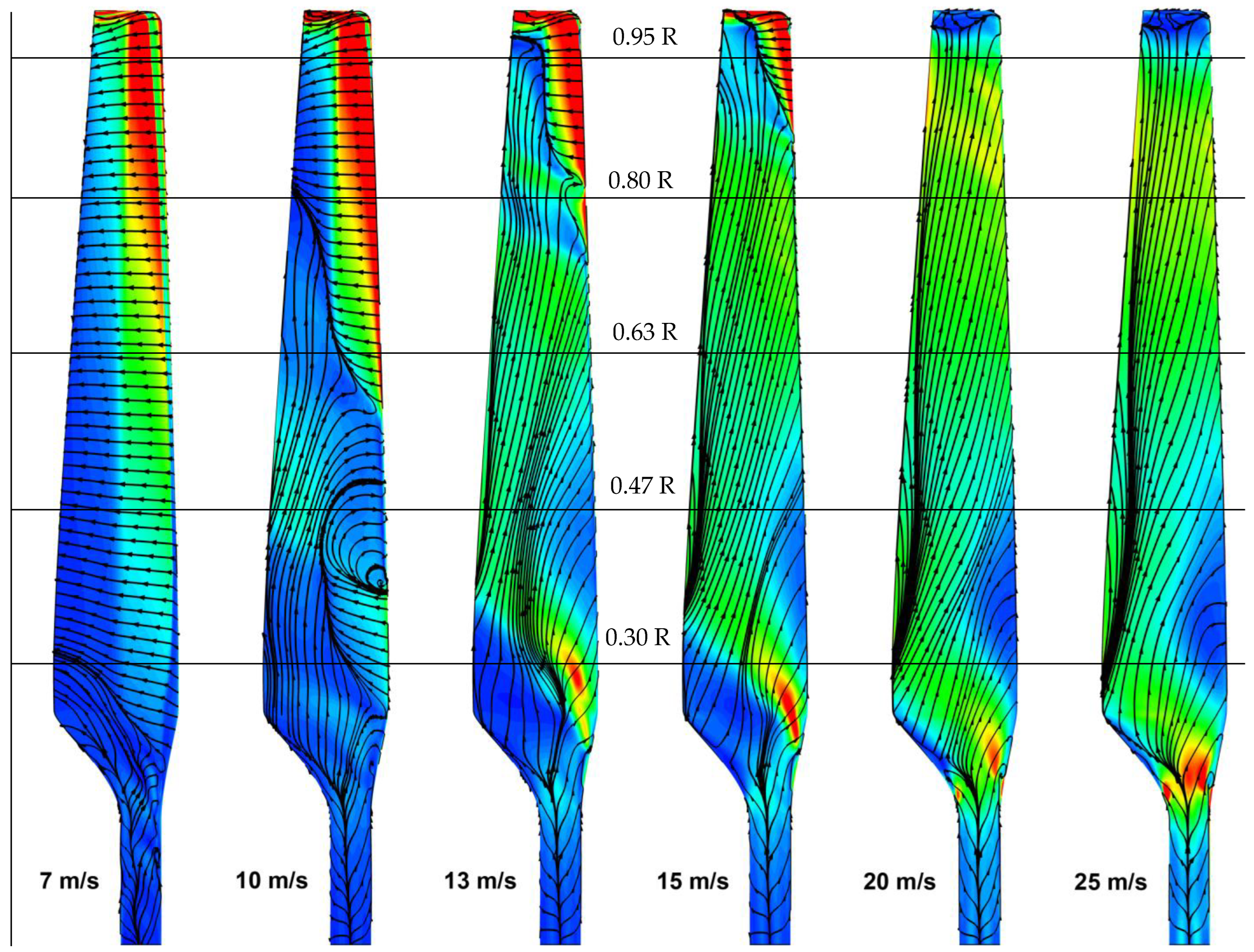
The results of the present study confirm that the attached flow regime is relatively straightforward, at least up to 7 m/s wind speed, with excellent predictions of all aerodynamic forces and moments. Between 7 and 10 m/s wind speed, the three-dimensional rotational effects become stronger, especially near the blade root, and approximately 10 m/s wind speed, an important part of the mid-blade section develops LE separation. From this point onwards, the separation quickly extends both up and down the blade, covering almost the entire blade length with the exception of a small tip section at 15 m/s. Between 17 and 25 m/s wind speed, the blade is fully stalled, the near-wall flow on the suction side running from root towards tip and from TE towards LE. The described processes can be readily observed in Figure 8, where oil-flow streamlines combined with wall shear stress (WSS) magnitude contours clearly show the boundary layer state on the blade suction side; the images were extracted at the same six wind speed values selected for the 2001 blind test.

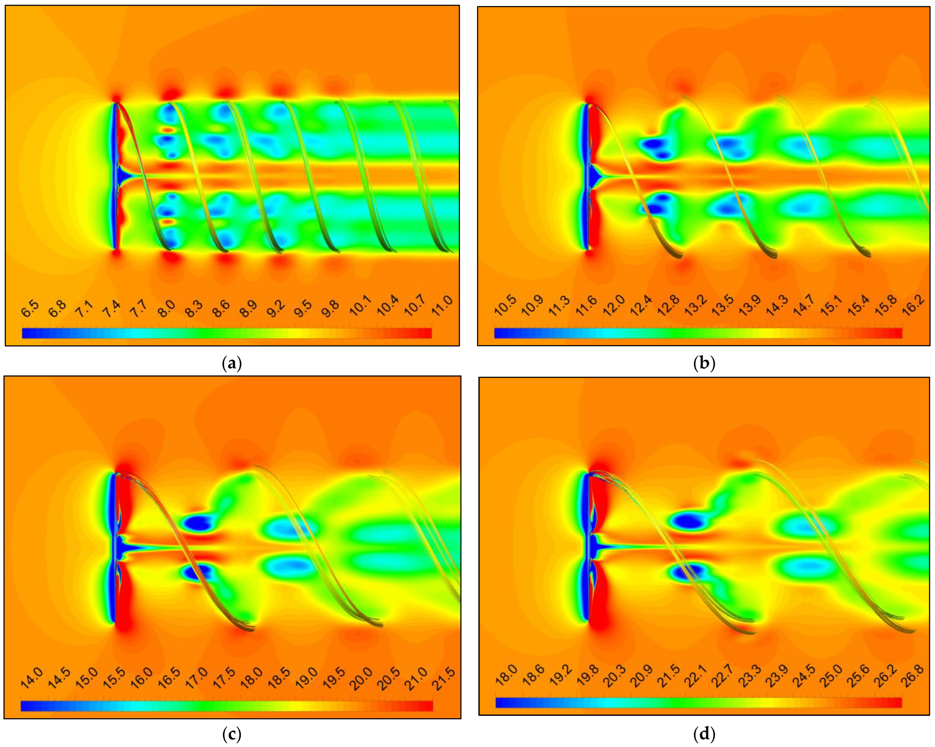
The development of the rotor wake structure with increasing wind speed can be examined in Figure 9. At 10 m/s, the wake is still relatively uniform, with two low-velocity traces left by the LE separation and the blade tip vortex. The vortical structures are well propagated downstream, and become progressively less distinguishable after approximately three blade lengths. At all other wind speeds the wake is highly non-uniform, with alternating high and low velocity regions, progressively skewed towards outlet with increasing wind speed. The streamlines released from the blade tip picture very distinctively the rotor tip speed ratio (TSR) drop from 10 m/s (3.79) to 25 m/s (1.52) wind speed.

The third parameter taken into consideration was the blade root flap bending moment (Channel ID: B3RFB), which was directly measured using strain gauges placed at a radius of 0.432 m from the axis of rotation. Both the measured B3RFB moment and the estimated aerodynamic moment (ID: EAERORFB), determined using the pressure measurements and the teeter link force, were included in the CFD data analysis for a more comprehensive comparison.

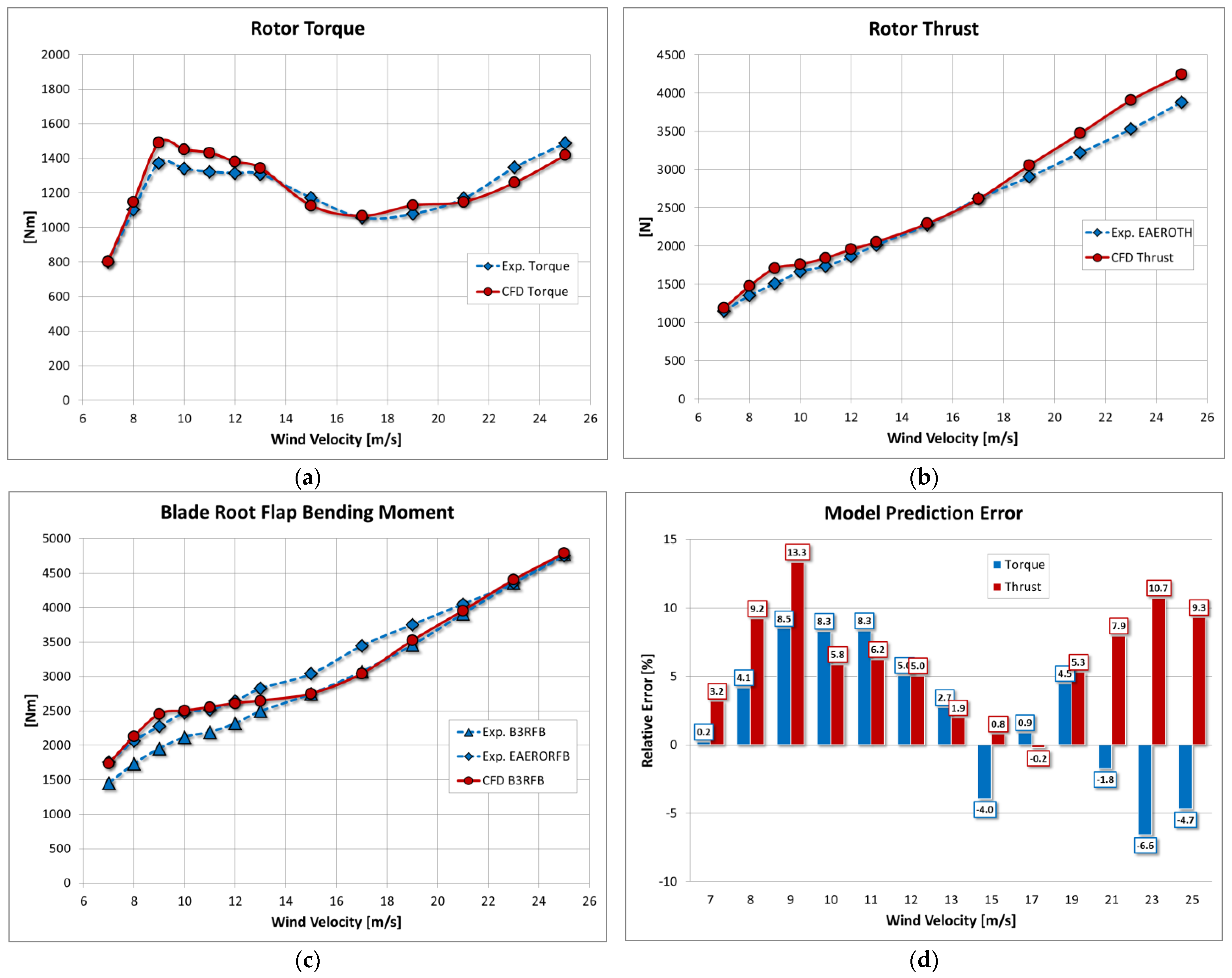
Examining the global aerodynamic forces and moments data comparison between CFD and experiment (Figure 10) the first thing to notice is that generally, the agreement is quite good, particularly when considering the results of the foregoing studies which used similar approaches, including our own previous work on the subject.

The predicted rotor torque at low wind speed is very accurate (error is less 1% of the experimental value), and that is strongly confirmed by the analysis of pressure coefficient (Figure 11) and thrust and torque coefficients (Figure 12) comparison with experimental data. Evidently, the predicted normal aerodynamic force component is also very accurate.

The primary transition zone (8 to 13 m/s wind speed) is characterized by an over-prediction of rotor torque, which tends to peak around the stall initiation point (9 to 11 m/s wind speed). The CFD rotor thrust largely has the same trend, with a maximum deviation at 9 m/s, followed by an increasingly better agreement with the estimated thrust.

The secondary transition zone (up to approximately 17 m/s) and the fully separated flow zone (up to max. wind speed) show a fluctuating rotor torque error, alternatingly above and below the measurements. The numerically simulated rotor thrust is very close to the estimated data in the final part of the transition zone, but diverges beyond 17 m/s, reaching approximately 10% over prediction towards the end of the test matrix.

The blade root flap bending moment (BRFB) analysis reveals a very intriguing situation. If we restricted the comparison to the experimentally measured data, the results of the numerical simulation up to 15 m/s wind speed would be overestimated by quite a significant margin, with a maximum at 9 m/s (+25%), but almost exact afterwards. Alternatively, if we considered only the estimated root flap bending moment, computed using the pressure data, the agreement would be very good except between 13 and 21 m/s wind speed, where it would be underestimated, most significantly at 17 m/s (−12%). Combining the two experimental curves with the CFD results is rather curious (Figure 10c). We do not have an explanation for this, but we are assuming that the transition from fully-attached flow to fully stalled flow plays a very important part—interestingly how the CFD curve gradually switches from estimated BRFB moment to the measured BRFB precisely during this transitional wind speed range.

Another strange observation is the apparent discrepancy between the very good BRFB moment prediction at high wind speed and the significantly poorer estimation of rotor thrust under the same conditions. Taking into account the fact that experimental thrust data was not directly measured, but estimated a posteriori, we must maintain a certain degree of reservation regarding its accuracy.

Finally, in our opinion, a correct assessment of a particular modeling approach based on the NREL Phase VI rotor should not be restricted to the six main cases of the initial blind test. A truly accurate image about the performance of the numerical model may be obtained only by testing it against the full experimental data spectrum, in detail, particularly over the stall initiation & propagation wind speed range (from 9 to 13 m/s).

3.2. Calculated Aerodynamic Coefficients Analysis

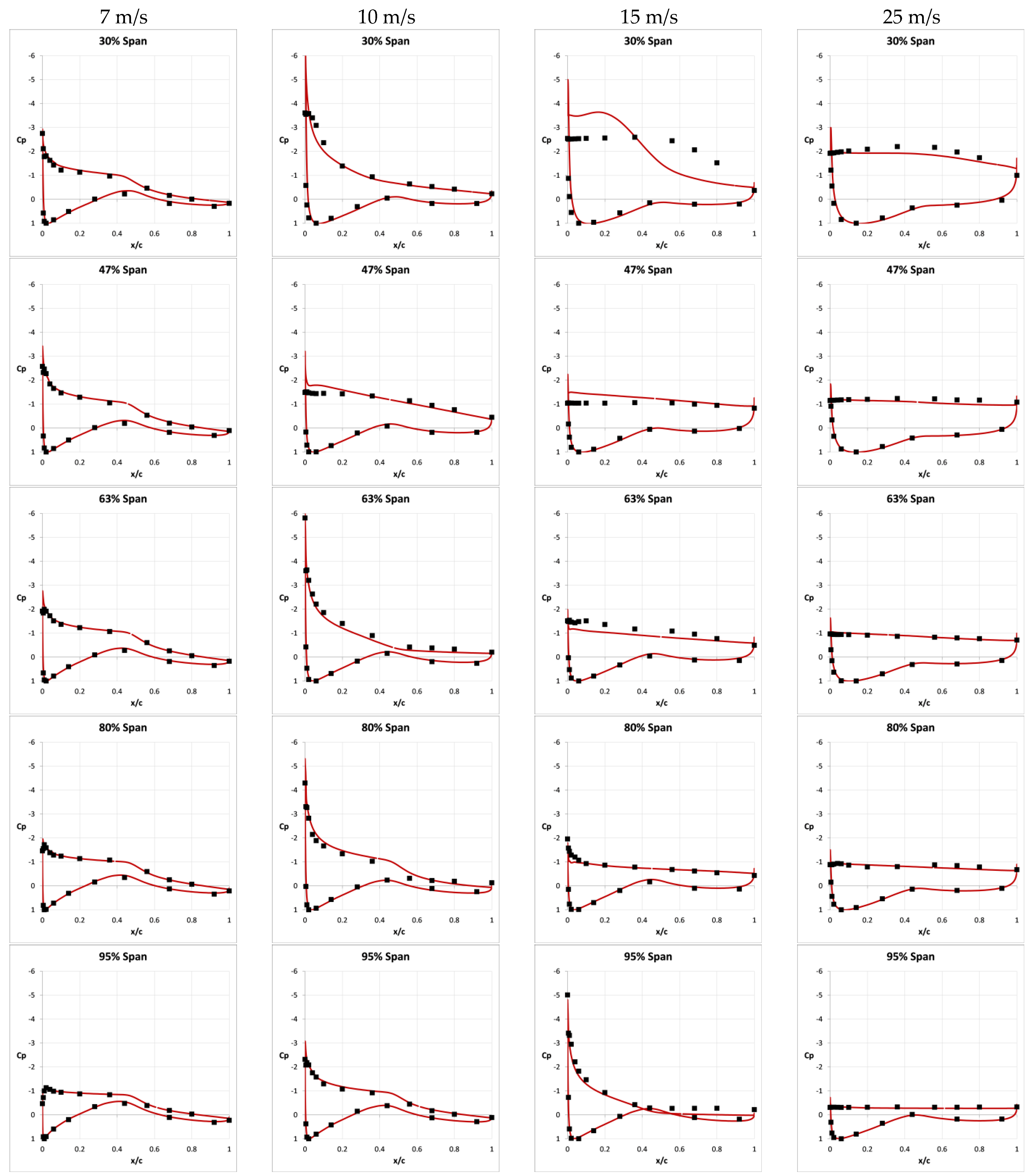
In order to assess the quality of the numerical predictions in more detail, the local distributions of pressure coefficient and the associated force and/or moment coefficients must be discussed. We have selected four wind velocities (7, 10, 15 and 25 m/s) to extract pressure coefficient plots at the same five radial stations on the blade that were used experimentally (see Figure 3). The calculation procedure is given in Appendix A, Equation (1), and the extracted results are presented in Figure 11. The scale of the Y-axis (representing C_p) used in the graphical representations was intentionally inverted and made identical for all plots (+1 to −6) to facilitate the direct analysis and comparison of the flow properties at all blade sections and all wind speeds at the same time.

We observe that the calculated pressure distribution on the pressure side of the rotor blade is very close to the measured one. There are some slight deviations, more notably between the stagnation point and the LE that are more visible at the root section (r/R = 0.3), but nothing obvious otherwise. We can conclude that the upwind pressure field is very reliably predicted, regardless of the operating conditions.

The analysis is not so straightforward on the suction side, though; we shall concentrate on this in the following comments. At the two extreme cases, the numerical estimation precision is quite remarkable. At 7 m/s wind speed, the flow is attached over the entire active section of the blade—although the influence of the blade root geometry and rotational effects start to make their presence felt (see Figure 8). This is very clearly evidenced in the numerical results also, with near-perfect match to the measured data. This also translates into excellent evaluation of rotor performance and blade loads. At 25 m/s, the flow is fully separated on the suction side. The numerically calculated curves do not follow the measured values without deviation, but the correlation is very good. The root section (r/R = 0.3) pressure distribution unmistakably show the lift augmentation effect induced by rotation (average abs. C_p > 1.5), while the tip section (r/R = 0.9) is strongly affected by local losses, with markedly reduced lift (average abs. C_p < 0.5). Overall though, the estimated rotor performance at this wind speed is only acceptable; the rotor torque is underestimated by 4.7% and rotor thrust is overestimated by 9.3%; only the blade root bending moment numerically calculated value is satisfactory. Probably the integrated quantities are very easily affected by minute inaccuracies and the high wind speed greatly amplifies their effect. Furthermore, the actual flow is highly unsteady and three-dimensional on the suction side—less-than-ideal conditions for RANS modeling.

At 10 m/s wind speed, blade stall is observable around the r/R = 0.47 station in the measure data. The numerical model proves sufficiently sensitive and manages to pick that up, but deviates somewhat near the LE, raising C_p to approximately −2, whereas experimental values top off at −1.5; both values denote significant rotational lift augmentation. At root, there’s a similar situation in the sense that the prediction is very good on the last three quarters of the blade, but differs on the front quarter—the model indicates attached flow while the measurements suggest a LE-attached local vortex. The 63% span section partial separation is a little too strong in the model results, whereas the separation is under-predicted at r/R = 0.8 and blade tip. This is the main reason for the higher numerically calculated rotor torque and thrust values.

The root section flow at 15 m/s is not particularly well reproduced by the model. It predicts a large, standing vortex occupying the first half of the blade width, followed by an almost flat, separated flow along the second half. The experimental data implies that the LE vortex is in fact weaker and diffused over almost the entire blade width. The calculated C_p peaks at approximately −3.5, while the measured C_p barely exceeds −2.5. At 47% blade span, the C_p distribution corresponds to a fully separated flow, just as observed in the experimental setup, but it is slightly optimistic, over-predicting the LE value by 0.5. The 63% span location is also dominated by separated flow; the numerical model evaluation suggests a stronger separation than observed in the wind tunnel. Apart from a zone immediately behind the LE, the 80% station results are quite closely following the measurements. At the blade tip, there is a notable underestimation of the rotational component in the separated flow region over the second half of the blade width. As far as the rotor performance is concerned at this wind speed, only the calculated rotor torque is lower than in the experiment by 4%, other quantities are very well determined.

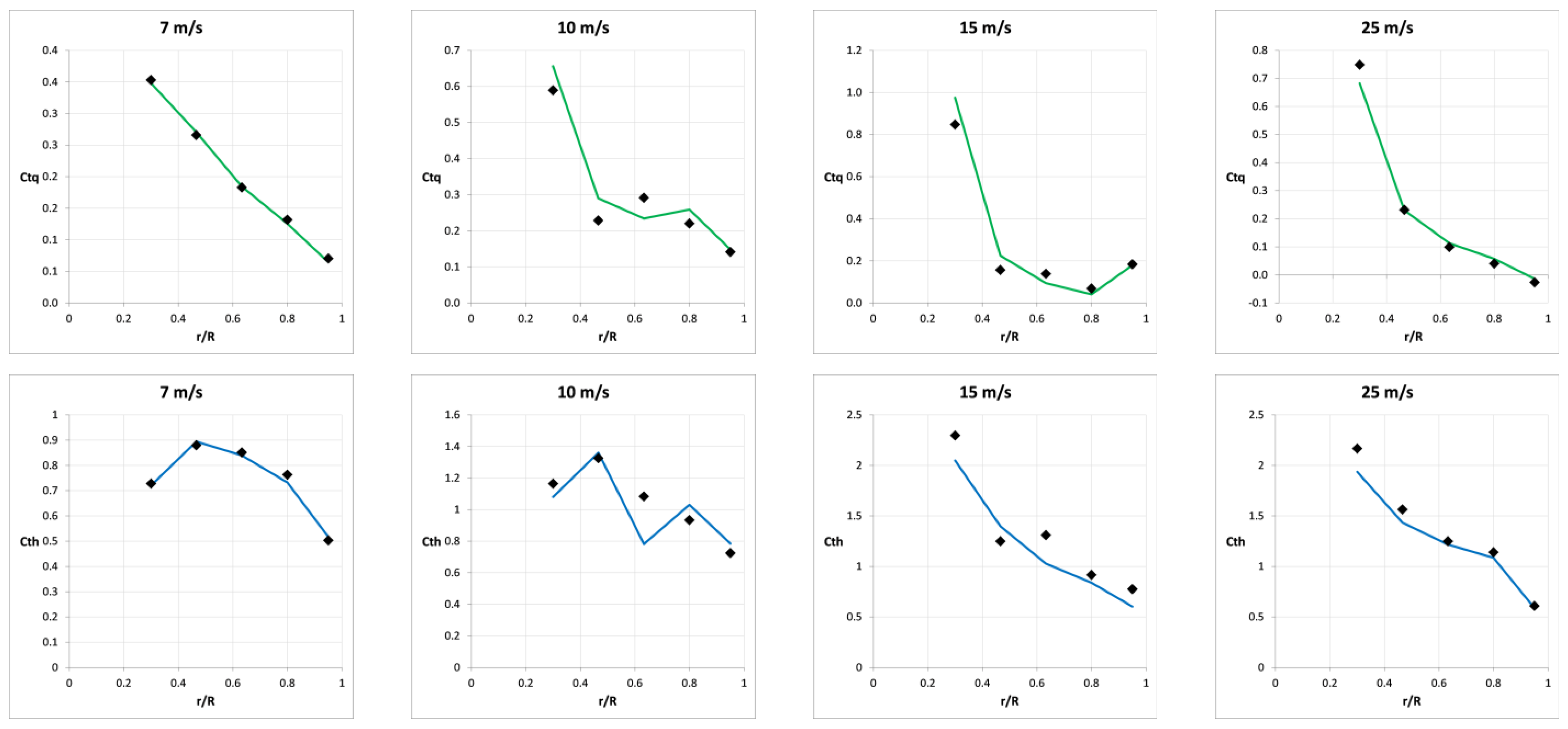
The blade spanwise distribution of torque and thrust coefficients is presented in Figure 12. The numerical data was calculated based on the methodology described in Appendix A, using Equations (2) and (3). The Y-axis scale used for these plots is not the same because it was considered important to allow the reader to more easily observe the relative errors.

The observations made in the above pressure coefficients analysis are well reflected in these plots. The 7 and 25 m/s cases are remarkably well reproduced numerically, especially the low wind speed case. For the highest wind speed case, obvious deviations can only be noted at the blade root. The mid-range cases (10 and 15 m/s wind speed) show a reasonable agreement between numerical model results and measurement; blade extremities seem to be better estimated compared to the intermediate sections. Still, the trends are qualitatively correct, in all cases.

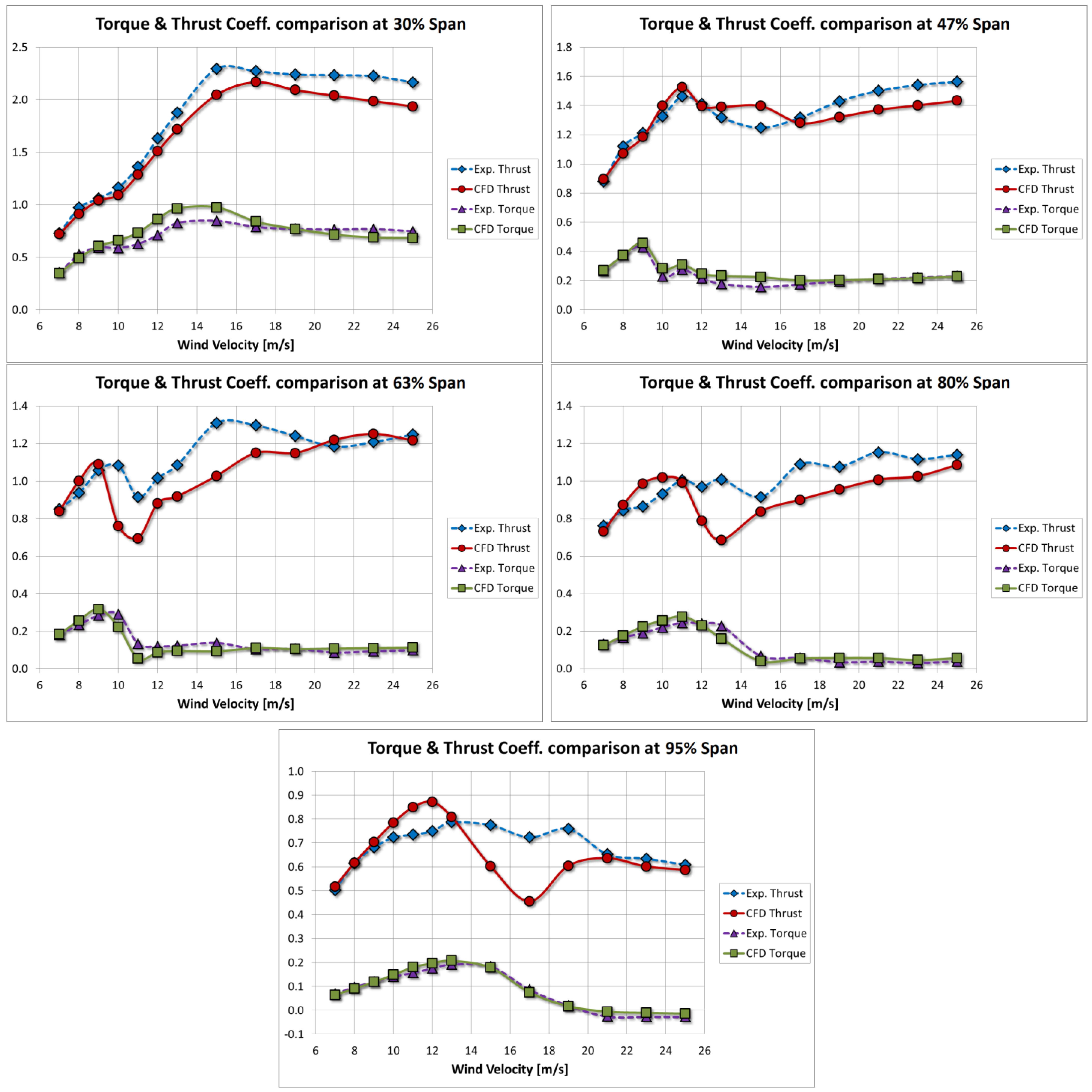
It is also very interesting to see how these force coefficients behave over the entire experimental wind speed range. For this purpose, Figure 13 includes plots of thrust and torque coefficients against wind speed for each of the five blade radial stations, representing a comprehensive comparison of numerical data vs. measurement-derived data.

Torque coefficient (C_tq) is generally quite well estimated, not much else to say about that. The relative errors are significant locally in the 10 to 17 m/s wind speed region at the first four sections (from root to tip), but the tendencies are very consistently captured. At blade tip (r/R = 0.95), torque coefficient prediction is best.

Despite the fact that pressure coefficient distribution at the 30% and 47% blade span sections is something that can be improved, numerical thrust coefficient (C_th) variation with wind speed at the same locations is more than acceptably computed. The relative errors are decent, even small at low wind speeds (up to approximately 13 m/s). Some underestimation is visible at higher wind speeds, and it is consistent. At the 63% blade span section, up to 9 m/s and beyond 20 m/s, the numerically calculated values are very good; but in between, only the trend is captured to some degree; there are large deviations approximately 10 and 15 m/s wind speeds. The behavior of the numerical results at the outboard blade sections contains strange artifacts, which we do not have an explanation for: a peak and a dip are observed in each of the two curves, considerably more pronounced at the 95% blade span section, that have no clear counterpart in the experimental measurements. Topologically, these features are similarities to the 63% blade span section qualitative development, as observed both numerically and in the wind tunnel experiments, but they cannot be seemingly identified in the corresponding measured data at the outboard sections. Strangely though, these apparently large errors do not seem to have a discernible influence on the global rotor performance as numerically determined—the mid-range calculated values are very close to the measurements, for all quantities.

3.3. Blade Stall Prediction Analysis

One of the key aspects of a stall-regulated wind turbine operation is the very initiation and development of stall phenomenon. As demonstrated by the results, the numerical model created for the present study is very successful by predicting with great accuracy the blade stall initiation, which occurs somewhere between 9 and 10 m/s wind speed.

Due to its geometrical particularities, the S809 airfoil features a two-stage stall. According to [3], at the Re number particular to the NREL Phase VI wind turbine (≈ 1 × 10⁶ at the blade tip), the first stage is a turbulent TE separation, which begins approx. when the upper limit of the laminar bucket is crossed (α ≈ 6°), and slowly increases with increasing AOA. After almost reaching the maximum design lift (C_l = 0.97, at α ≈ 9°) the separation point advances rapidly from TE towards LE and stabilizes approximately mid-chord (α ≈ 11°). 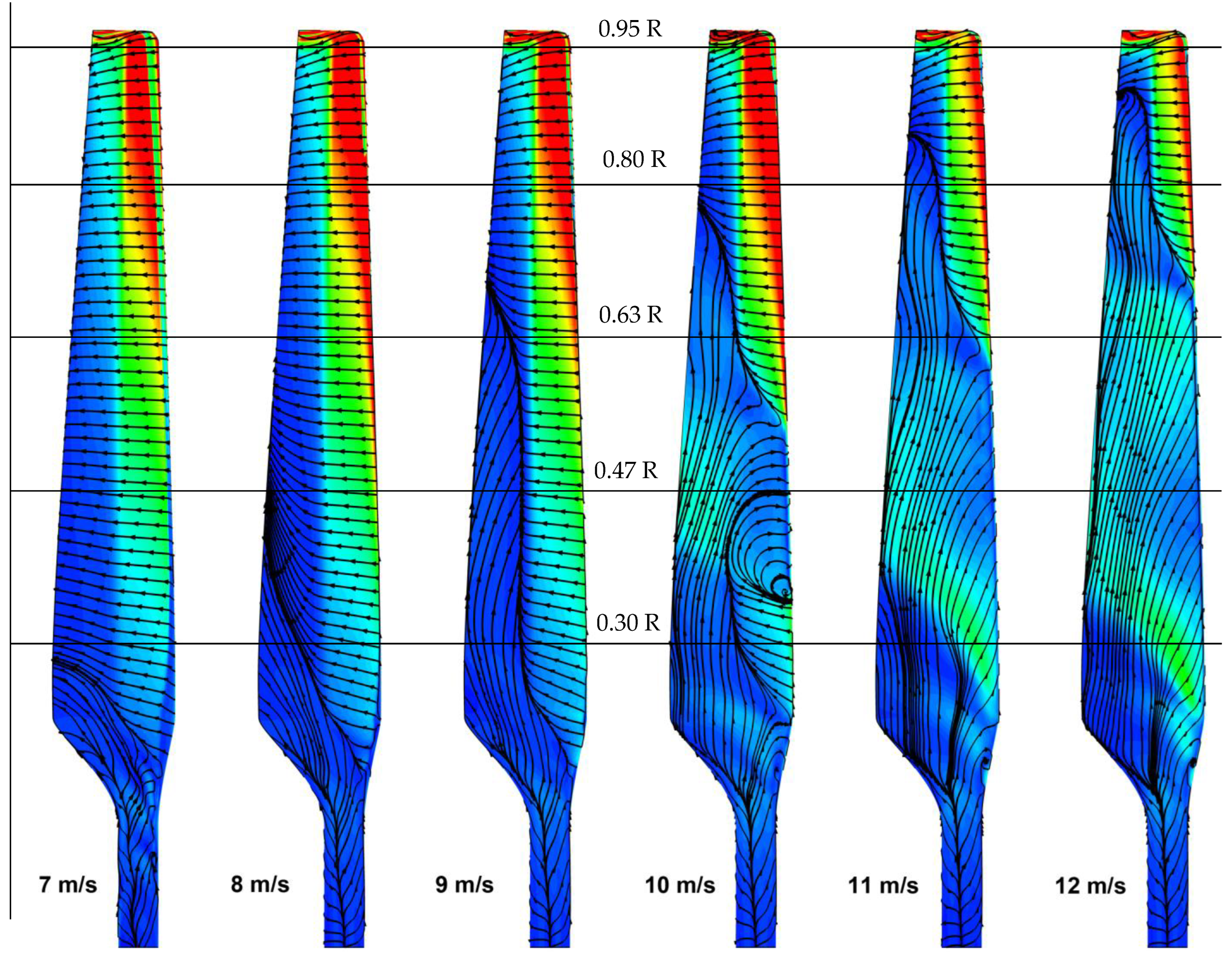The separation point remains practically fixed until the maximum lift is obtained (C_l = 1.06, at α ≈ 15°), which marks the end of the first stall stage. As the angle of attack is increased further, the second stall stage begins, with the separation point quickly migrating forward again, towards the LE. These particularities can be easily identified in the evolution of the suction side NREL blade stall, as presented in Figure 14. Please note that the state of the boundary layer flow is materialized in the pictures by the oil-flow streamlines, while the WSS magnitude contours are only added to enhance the representation and supplement the qualitative analysis.

At 7 m/s, only a slight TE separation at the blade root and over the transition piece can be seen, with obvious effects on the wall-limiting streamlines, deviated spanwise by the centrifugal and Coriolis forces. At 8 m/s, the TE separation advances towards the blade tip, while the rotational forces noticeably affect more than half of the aft part of the suction side. At 9 m/s, a complete boundary layer (BL) separation takes place between the blade TE and the mid-chord line, over two-thirds of the blade length. There is no evidence of any LE separation yet. The separation line is very clearly defined.

The 10 m/s wind speed marks the occurrence of blade stall. Judging by the size of the separation zone and by, for example, the shape of rotor torque curve, it is very likely that the LE separation actually starts sooner, probably closer to the 9 m/s wind speed. This is quite remarkable, because generally this feature has been proven to be very difficult to reproduce numerically by most of the CFD studies of UAE rotor. Some of the authors noted the large inaccuracies of their numerical results when compared to the experimental data at this particular wind speed, specifically for the 47% span section [8].

Measured at the LE, the stalled section starts at r/R = 37% and ends at r/R = 57%, which places the 47% span section right in the middle. Interestingly, there still is a blade section below which is not yet stalled. This could be interpreted as a stall delay phenomenon caused by the rotational effects predominant in this region of the blade. The TE separation extends to approximately 81% of the blade length.

Further increasing the wind speed to 11 m/s moves the upper boundary of the LE stall section to r/R = 63%, while the entire non-stalled region at the blade root is replaced by a vortex, which crosses the blade diagonally up, from the LE to the TE. The attached flow zone and the stalled zone are separated by a very pronounced inverted S-shaped line.

At higher wind velocities, the separation line advances towards the blade tip until it disappears entirely as the separated flow region occupies the whole suction side, and the root vortex continues to grow in intensity up to approximately 15 m/s, slowly decaying afterwards (see Figure 8).

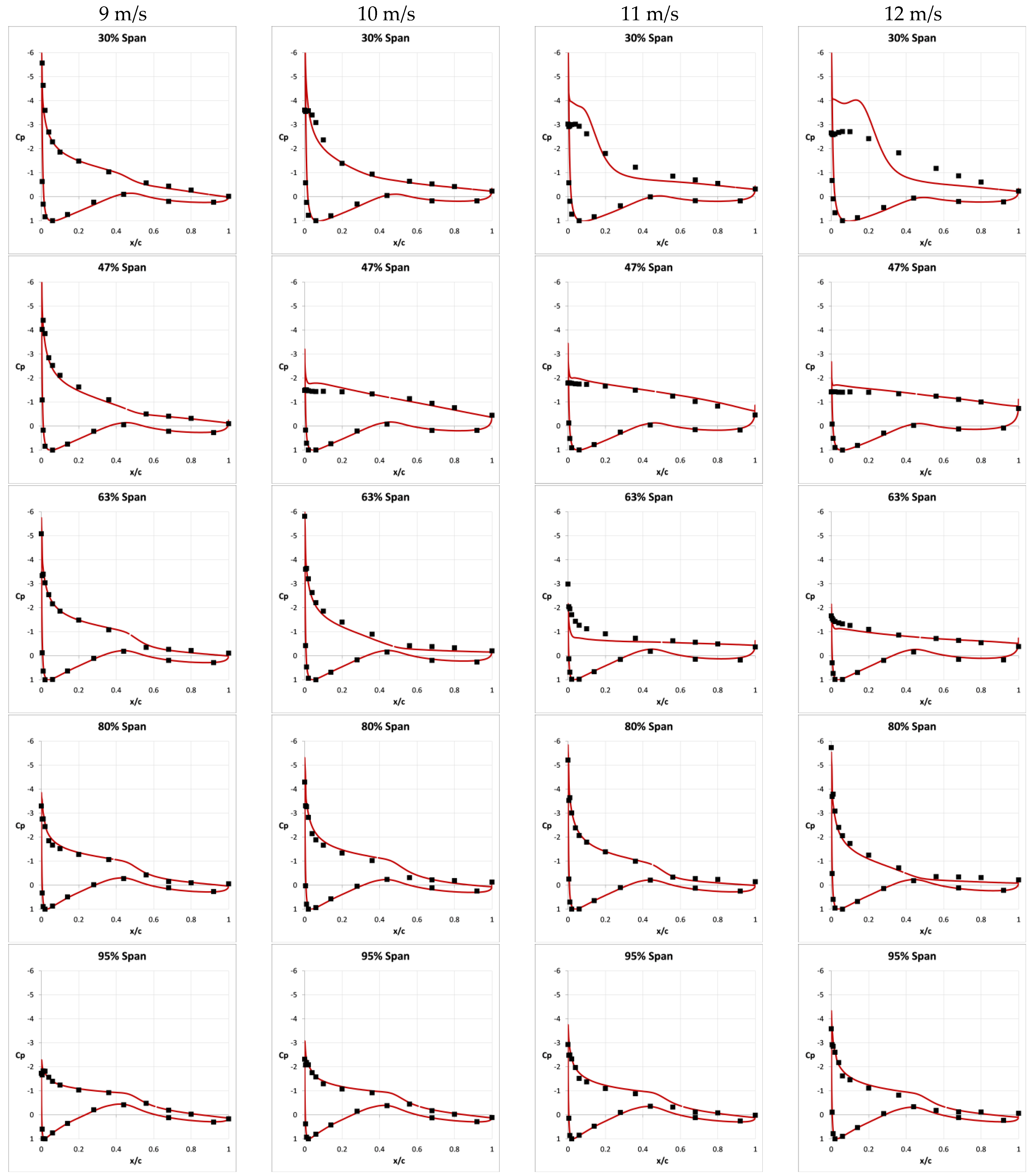
The pressure coefficient distribution for the 9 to 12 m/s wind speed cases is presented in Figure 15. The surface streamlines in Figure 14 definitely show the TE separation at 9 m/s. On the other hand, a close analysis of the pressure coefficient distribution numerically predicted for this wind speed reveals that, actually, the CFD model separation is not strong enough—the 95% blade span section is the exception. This is the main reason for the overestimation of rotor torque and thrust at 8 and 9 m/s wind speed. It looks like the turbulence model sensitivity to adverse pressure gradient is not sufficiently high under these conditions.

The 10 m/s case has already been discussed above (see Section 3.2). Since they are relatively similar, the results from 11 and 12 m/s cases are analyzed together below.

At r/R = 0.3 section, in accordance with the observations made for the 15 m/s case, a standing vortex forms, attached to the blade LE. In both 11 & 12 m/s cases, the measured pressure field reveals a lower intensity vortex, more broadly distributed in the chordwise direction than the vortex present in the numerical results. It is not clear if this feature is tied to the turbulence modeling, or it is perhaps related to the modeling inaccuracies of the blade root transition piece. Specific numerical test could be conducted in future research to shed light on this matter. The model results agree very well with the wind tunnel measurements at r/R = 0.47 blade section. Only little inconsistency can be found near the LE, though significantly less than in the 10 m/s wind speed case. At r/R= 0.63, the separation is too strong, again, in the simulation; the calculated 12 m/s wind speed case pressure field is not far from the measurements as a matter of fact, but the 11 m/s results are dissonant, to a similar degree as noted in the 10 m/s case. At 80% blade span, results are mixed: the 11 m/s wind speed case shows good correspondence with physical observations, but the 12 m/s case results suffer from too much separation in the first half, and too little in the second half of the blade section. The 95% blade span section prediction is reasonably good in both cases, albeit some over-prediction can be noticed over the first half.

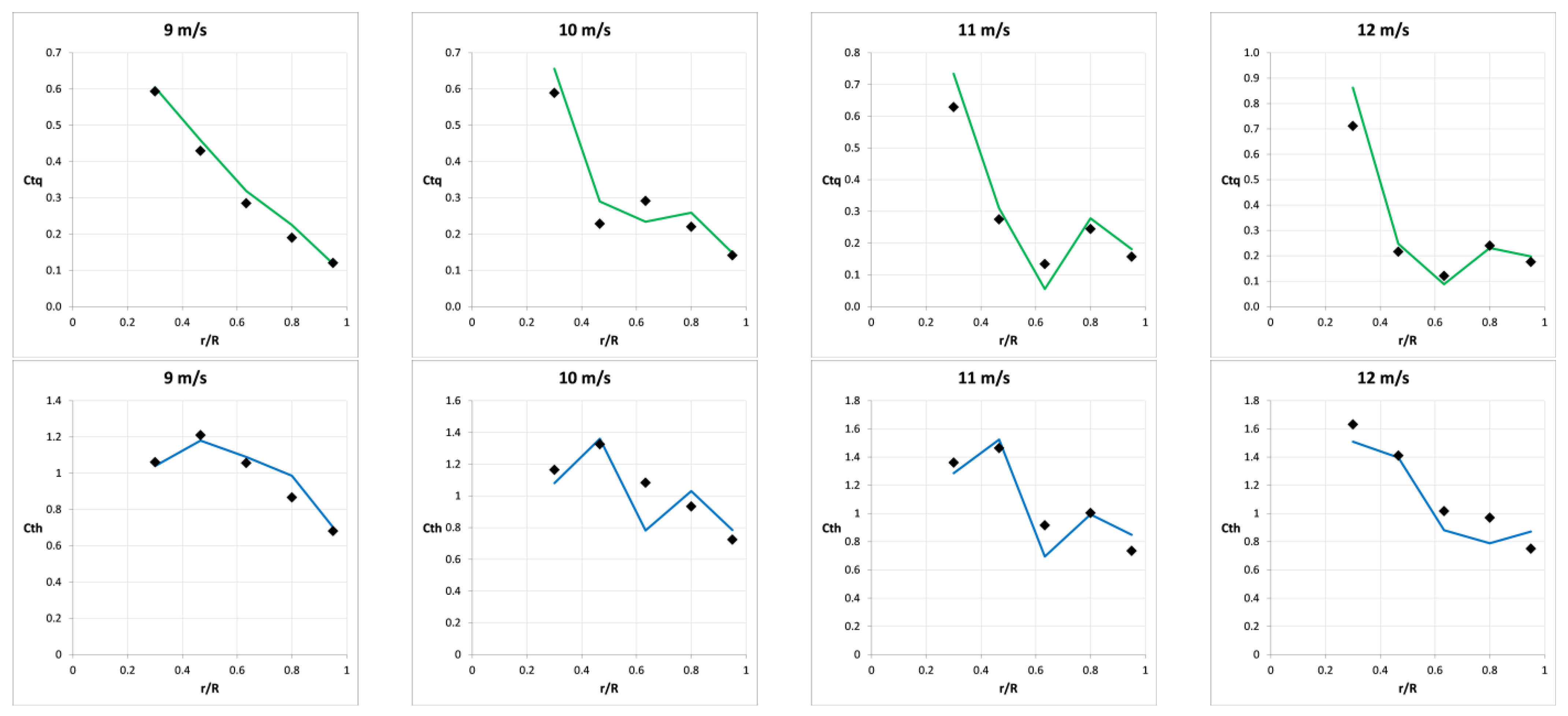
Figure 16 shows the distribution of torque and thrust coefficients on the blade in the radial direction for the same four wind speeds. The remarks made above can be immediately correlated with the information contained in these plots. Once more, in general, the trends are captured by the model acceptably well; the 63% and 80% blade length sections look to be the most problematic ones. Obviously, that has a direct impact on the accuracy of the rotor performance calculation, because these sections are located towards the blade tip.

4. Discussion

As long as the flow remains mostly attached to the blade suction side, the results obtained from the CFD model calculations are very good. At the other end of the tested operating conditions spectrum, i.e., high wind speeds, the situation is again favorable for the CFD model; it is capable of estimating quite well the pressure field around the turbine blade under fully separated flow. Some discrepancies can be identified when assessing the rotor performance, which underline the susceptibility of the global forces and moments to slight errors in local predictions, but qualitatively the numerical results look very convincing. In between, the level of precision is variable. A definitive conclusion is difficult to formulate in this regard and, without a doubt, improvements need to be made. Nevertheless, the numerical model and the simulation methodology proves its value by reproducing with more accuracy then most previous published research using comparable approaches the initiation and propagation of blade stall phenomena. Considering that this particular turbine was designed to be stall limited, even the qualitative prediction of stall is of great importance.

Surely, apart from the blade twist and taper, the blade stall characteristics are heavily influenced by the properties of the airfoil used for its construction. The S809 airfoil does have some particularities, compared to the typical airfoil used in, let us say, aircraft wing design, which might be more favorable to CFD modeling—one might argue. Even so, the previous works plainly demonstrate that is not necessarily true, or that to the very least it should not be taken for granted, as the CFD approach does not perform satisfactorily for the NREL Phase VI rotor with most turbulence models or model construction techniques. Nor do other approaches, for that matter.

The overall modeling and simulation cost is very much acceptable, in our opinion. CFD is not a simple procedure by definition; however, putting this work into perspective, there are applications for CFD that are much more challenging to handle that way. The modeling phase is, by far, the most difficult. Very precise geometric modeling is paramount, because the numerical results are known to be extremely sensitive to local errors for flows over aerodynamic surfaces. A good fidelity in terms of model geometry vs. actual, tested geometry, blade root and blade tip reproduction, etc., could have a big impact and make the difference between success and failure. That being said, still the mesh construction is the most problematic stage, and we believe it is the true cornerstone for wind turbine modeling.

The meshing techniques employed for this study require a high level of proficiency and are time-consuming—more than half of the total effort was dedicated to the mesh building stage. Adding to that the fact that changing the blade angle, or tuning the twist distribution are not trivial tasks with fully structured meshing—although, mesh morphing or other, similar methods can be used to conform an existing mesh to the new shape—the appeal for such solution is understandably low. These issues also raise difficulties for engineering design processes, which is the main target for our research. Unstructured meshing, on the other hand, as user-friendly and accessible as it is, did not prove to be a viable alternative yet. Our firm observation is that the near-blade mesh region must be very carefully executed; it must be of very good quality as far as mesh metrics are concerned, and also ensure enough nodal density in all directions, including spanwise, but most importantly in the boundary layer. At the same time, this mesh zone must extend over a significant normal distance, perhaps even up to one chord away, thus avoiding mesh topology changes, abrupt cell sizing variation, numerical interfaces, or other disruptions to be placed too close to the blade surface. Such construction is extremely difficult or quite impossible to achieve with existing unstructured layering techniques. To conclude this idea, most probably a hybrid approach might be ideal: combining the suggested, fully structured mesh zone enveloping the turbine blade(s) with a volume-filling unstructured method, also using mesh refinement in the rotor wake.

Lastly, the simulation and data post-processing stages were rather uneventful and did not involve too much effort. With the available computing power, the time spent would be in the order of days for the work presented herein. Therefore, in our view, the main goal of this research was attained.

One possible direction to develop the present work would be to address the issues of turbulence modeling. Most importantly, given the relatively low Reynolds number of the flow for the testing conditions (blade root Re ≈ 3 × 10⁵, blade tip Re ≈ 1 × 10⁶) and the experimental evidence available for the S809 airfoil testing, the inclusion of boundary layer transition modeling could be worthwhile, even though other researchers did not obtain remarkable results following this path. Higher mesh resolutions, especially on the blade surface and, implicitly, in the boundary layer might also be tested. This can improve the response of the model to local unsteadiness in the stalled flow and possibly correct some of the observed deficiencies, or even allow for scale-resolving turbulence modeling.

All these research directions can bring potential benefits for the realization of improved methods for the numerical simulation of any type of wind turbine. The offshore applications are specifically targeted due to their higher energy potential, more favorable operating conditions and increased interest for future development.