A Hybrid Dynamic Method for Conflict-Free Integrated Schedule Optimization in U-Shaped Automated Container Terminals

Abstract

Automated guided vehicles (AGVs) in the U-shaped automated container terminal travel longer and more complex paths. The conflicts among AGVs are trickier. The scheduling strategy of the traditional automated container terminal is difficult to be applied to the U-shaped automated container terminal. In order to minimize the handling time of all tasks and avoid AGV conflicts simultaneously in the U-shaped automated container terminal, this paper establishes a hybrid programming model for conflict-free integrated scheduling of quay cranes, AGVs, and double-cantilever rail cranes in the unloading process. It consists of a discrete event dynamic model and a continuous time dynamic model. An improved genetic seagull optimization algorithm (GSOA) is designed. A series of numerical experiments are conducted to verify the effectiveness and the efficiency of the model and the algorithm. The results show that the proposed method can simultaneously realize the AGVs collision avoidance and multi-equipment integrated scheduling optimization in the U-shaped automated container terminal.

1. Introduction

As the connection point between land transportation and sea transportation, container terminals play important roles in commodity transportation. With the development of economic globalization and the growth of vessels, the throughputs of container terminals are constantly increasing. Multiple partners in the port and shipping supply chain put forward higher requirements for the handling efficiency and automation level of facilities in container terminals. A traditional automated container terminal usually has a vertical layout. Its construction cost is high. It usually adopts the end handling, and automated guided vehicles (AGVs) and external trucks only need to drive into the seaside and landside ends of the blocks in the yard, respectively. Non-cantilever rail cranes are the main yard equipment. They have to travel a long distance with containers to complete the handling. It results in high energy consumption and low efficiency. However, the emerging U-shaped automated container terminal (as shown in Figure 1) adopts side handling. The container handling points are longitudinally set on both sides of the blocks. AGVs and external trucks can travel into the yard. Double-cantilever rail cranes in the yard interact directly with AGVs or external trucks. A U-shaped automated container terminal hahas the advantages of a high efficiency and low cost, which is the transformation direction of traditional container terminals.

Nowadays, multi-equipment integrated scheduling and AGV path planning have become the main research topics in container terminals. During the actual operation, uncertain environments may cause collision and congestion problems in AGV path planning. In the U-shaped automated container terminal, AGVs need to travel longer distances for loading and unloading in the yard. This leads to the problem of mutual waiting between the AGV and double-cantilever rail crane, which affects the overall handling efficiency in the U-shaped automated container terminal. In order to solve these problems and improve the loading and unloading efficiency of the U-shaped automated container terminal, this paper takes the unloading process of the U-shaped automated container terminal as the research object. We establish a hybrid dynamic model for multi-equipment integrated scheduling based on bi-level programming. It is composed of a discrete event dynamic model and a continuous time dynamic model.

This paper has three main contributions:

(1)

According to the actual operational needs, this paper considers AGVs’ conflict-free path planning and multi-equipment integrated scheduling simultaneously instead of studying them separately.

(2)

This paper establishes a bi-level programming-based hybrid dynamic model composed of a discrete event dynamic model and a continuous time dynamic model. It minimizes the handling time of all tasks and avoids AGV conflicts simultaneously.

(3)

This paper designs an improved genetic seagull optimization algorithm to solve the model. By comparison with the adaptive genetic algorithm and bi-level genetic algorithm, the proposed method is validated on small-sized and large-sized problems.

The remaining subsections of this paper are as follows: Section 2 reviews related research on AGV path planning and integrated scheduling of automated container terminals. Section 3 further analyzes the problem and builds the model. Section 4 presents a genetic seagull algorithm. Section 5 conducts small-scale and large-scale example experiments. Section 6 concludes the article and points out future research directions.

2. Literature Review

In recent years, there have been many studies on multi-equipment integrated scheduling and AGV path planning in automated container terminals, and significant research results have been achieved.

Integrated scheduling of different equipment is an inevitable and very important subject to improve the efficiency of automated container terminals. Zhong et al. [1] studied the integrated scheduling problem of quay cranes (QCs), AGVs, and yard cranes in the automated container terminal. Li et al. [2] considered that loading and unloading processes occurred simultaneously and the high correlations between devices. They established a new mixed integer programming model to analyze the allocation and integrated scheduling of terminal equipment. Chen et al. [3] transformed the integrated scheduling problem of the automated container terminal into a multi-equipment collaborative scheduling problem. They established a commodity network traffic model with traffic balance constraints of a yard crane and AGV. Luo et al. [4] studied the multi-equipment integrated scheduling problem in an automated container terminal. They built a mixed integer programming model with the goal of minimizing the berthing time of the ship according to the loading process and discussed the work efficiency of the single cycle and double cycle mode. They created an adaptive genetic algorithm (AGA) to solve this model. Zhen et al. [5] studied the integrated scheduling of quay cranes and container trucks in container terminals, proved that the integrated scheduling problem is NP-hard, and proposed some features to greatly reduce the computational complexity. Koster et al. [6] established new integrated stochastic models in which they analyzed the performance of overlapping loading and unloading operations. They captured the complex stochastic interactions among quayside, horizontal transportation, and stackside processes. Zhao et al. [7] studied the multi-equipment scheduling problem of QCs and AGVs in automated container terminals, considering the capacity limitation of the quay crane transfer platform, and carried out data experiments with Qingdao port as an example. Jamrus et al. [8] applied the flexible job shop scheduling problem to a semiconductor manufacturing system and constructed a particle swarm optimization algorithm based on the Cauchy distribution and operator. However, there are few studies on three types of equipment, and few studies have considered the waiting time between equipment. In addition, AGV is the key piece of equipment in automated container terminals. When studying the integrated scheduling problem, the conflicts among AGVs have not been considered.

AGVs are the main piece of equipment connecting QCs and yard cranes (YCs) in automated container terminals. There are a lot of related studies on AGVs in automated container terminals [9,10,11,12,13,14]. Ma et al. [9] proposed a shuffled frog leaping algorithm with a mutant process for AGV path planning in automated container terminals, which could increase the diversity of the population and improve the convergence speed. Waldemar [10] used square topology to describe the transportation network and proposed an AGV collision and deadlock prevention method based on the reserved chain. Xu et al. [11] considered the conflict of AGVs in automated container terminals and avoided conflicts by controlling the speed of AGVs. Yang et al. [12] established a bi-level programming model, which could avoid AGV conflicts and proposed a bi-level genetic algorithm (BGA). Keisuke Murakami [13] studied the scheduling and conflict-free path planning of AGVs in a flexible manufacturing system. He used a spatiotemporal network to simulate the discrete fractional linear programming problem and expressed it as a mixed integer linear programming problem. In addition, he also proposed an effective inequality to speed up the calculation. Zhong et al. [14] studied multi-AGV conflict-free path planning in integrated scheduling of automated container terminals. They established a mixed integer programming model to solve the AGV conflict and deadlock problems effectively. Tomas et al. [15] studied the energy consumption of trucks in container terminals. They evaluated the energy consumption according to the dynamic characteristics of trucks and different routes, and finally proposed a new control strategy.

At present, there are many studies on multi-equipment integrated scheduling in automated container terminals but few studies on the integrated scheduling of quay cranes, AGVs, and double-cantilever rail cranes under the layout of a U-shaped automated container terminal [16,17,18]. Li et al. [19] conducted detailed simulation research on different types of layout design to compare their terminal performance. Li et al. [20] studied hybrid scheduling of yard cranes, AGVs, and external trucks under the layout of a U-shaped automated container terminal. Additionally, few studies have considered AGV conflict-free path planning in the process of multi-equipment integrated scheduling optimization [20,21,22]. The presented studies usually study AGV conflict-free path planning and multi-equipment integrated scheduling optimization separately, which limits practical applications of the research results. In practice, these two problems are interactively coupled. In the U-shaped automated container terminal, AGVs need to travel a long distance to reach the target bay, which will create a mutual waiting between the AGV and double-cantilever rail crane. Additionally, their paths are obviously different from those of the traditional automated container terminal. Accordingly, conflicts among AGVs are becoming trickier. These unique characteristics of these U-shaped automated container terminal mean that the models for traditional automated container terminals cannot be directly applied to U-shaped automated container terminals, so our integrated scheduling optimization of quay cranes, AGVs, and double-cantilever rail cranes considering the conflict-free path planning of AGVs in the U-shaped automated container terminal is important and timely. It helps to improve the operation efficiency and reduce the transportation cost of the U-shaped automated container terminal.

3. Model Formulation

This paper focuses on the unloading process, and the research objective is to minimize the handling time of all tasks in U-shaped automated container terminals. This problem includes more complex discrete event dynamic programming and continuous time dynamic programming. Discrete events occur during container handling between different equipment while the dynamic handling status (such as speed, displacement) of continuous time occurs in discrete events. Therefore, the bi-level programming model composed of a discrete event dynamic model and continuous time dynamic model is established. The dynamic characteristics mainly involve the time when AGV arrives at each node, the strategy to avoid conflicts, and the process of handling containers. This model is divided into two parts: one is the integrated scheduling model, and the other is the AGVs path planning model.

3.1. Assumptions

(1)

The AGV lane is unidirectional.

(2)

AGV runs at an average speed, considering the impact of acceleration, deceleration, turning, empty, and load.

(3)

A safe distance can be maintained among AGVs.

(4)

Multiple AGVs serve multiple quay cranes and they do not fixedly serve a certain quay crane.

(5)

The maximum carrying capacity of each AGV is two twenty-foot equivalent unit (TEU). The QC and double-cantilever rail crane can each handle up to 2 TEU at a time.

3.2. Model Parameters

$N=\left\{1,2,3\dots ,u,p\right\}$: set of all containers.

$V=\left\{1,2,3\dots ,c\right\}$: set of all AGVs.

$Q=\left\{1,2,3\dots ,a,b\right\}$: set of all QCs.

$Y=\left\{1,2,3,\dots ,m\right\}$: set of all double cantilever rail cranes

$B_{mn}$: set of all bays, where $m$ represents yard and $n$ represents bay.

$N_a$: set of containers handled by quay crane $a$.

$S$: a dummy starting quay crane.

$F$: a dummy ending quay crane.

$O_s: Q\cup S$, set of all quay cranes plus the dummy starting quay crane.

$O_F: Q\cup F$, set of all quay cranes plus the dummy ending quay crane.

$O: Q\cup F\cup S$, set, including all quay cranes.

$G=\left\{1,2,3\dots ,g\right\}$: set of nodes in the path network, where $g$ represents the number of nodes.

$E=\left\{e_{21},e_{18},\dots ,e_{ij}\right\}$: set of links in a path network, $e_{ij}=\left\{i\to j:i,j\in G\right\}$ represents the distance between node $i$ and node $j$, also represents the link between node $i$ and node $j$.

$W=\left\{w_{1,21},w_{2,18},\dots ,w_{u,ij}\right\}$: set of travel time, $w_{u,ij}$ represents the time when task $u$ pass $e_{ij}$.

$D$: set of shortest paths and alternative paths that need to be sorted.

$T_w={\left[T_{w_1,ij},T_{w_2,ij},\dots ,T_{w_{u,ij}}\right]}^T$: set of time window function.

$t_{in,ij}={\left[t_{in,1,ij},t_{in,2,ij},\dots ,t_{in,u,ij}\right]}^T$: set of the time of AGV entering link $e_{ij}$.

$t_{out,ij}={\left[t_{out,1,ij},t_{out,2,ij},\dots ,t_{out,u,ij}\right]}^T$: set of the time of AGV leaving link $e_{ij}$.

$v$: the speed of AGVs.

$M$: a very large positive number.

$T_1$: the time when portal trolley of the quay crane takes the container from the transfer platform to the AGV.

$T_3$: the time when the double cantilever rail crane takes the container from the AGV to the target bay.

$P$: the number of turns in one path.

$n_d$: the number of links of path $d$.

$k_{ua}$: the time when the QC $a$ starts to handle the container $u$.

$T_{ua}$: the time when the main trolley of QC $a$ takes the container $u$ from the ship to the transfer platform.

$r_{ua}$: the time when portal trolley of QC $a$ put the container $u$ from the transfer platform to the AGV.

$h_{ua}$: the time when AGV transports the container $u$ to the designated bay.

$q_{ua}$: the time when the double cantilever rail crane reaches the designated bay of the container $u.$

${\theta }_{um}$: the target bay of the container $u$ which handled by double cantilever rail crane $m$.

$f_{ua}$: the finish time of container $u$.

$x_{uapb}$: if AGV handles the container $p$ of quay crane $b$ after completing the container $u$ of quay crane $a$, it is 1; otherwise, it is 0.

${\beta }_{uac}$: if the AGV $c$ handles the container $u$ of quay crane $a$, it is 1; otherwise, it is 0.

${\alpha }_{uamn}$: if the target bay of the container $u$ is bay $n$ in the yard $m$, it is 1; otherwise, it is 0.

$y_{ijc}$: if AGV $c$ passes through node $i$ and node $j$ in turn, it is 1; otherwise, it is 0.

$z_{ij}$: if AGV $c$ selects the link from node $i$ to node $j$, it is 1; otherwise, it is 0.

3.3. Design of the Upper-Layer Model

$$\min T=\underset{u\in N_a}{\max }{f}_{ua}-\underset{u\in Na}{\min }{k}_{ua},\forall a\in O$$

(1)

In this paper, the multi-equipment scheduling system is regarded as a discrete event dynamic system [22,23]. Equation (1) is the objective function of the model, which aims to minimize the handling time difference between completing the last container and starting the first container, which represents the total completion time of tasks:

$$k_{ua}+T_{ua}+T_1\le r_{ua},\forall u\in N_a,\forall a\in O$$

(2)

$$r_{ua}+{\displaystyle \sum }_{c\in V}{w}_{i,j}·{\beta }_{uac}\le h_{ua},\forall u\in N_a,\forall a\in O,\forall i\in O,j\in B_{mn}$$

(3)

$$\max \left\{h_{ua},q_{ua}\right\}+T_3{\displaystyle \sum }_{m,n\in B_{mn}}{\alpha }_{uamn}\le f_{ua},\forall u\in N_a,\forall a\in O$$

(4)

$$\begin{array}{c}\max \left\{h_{ua},q_{ua}\right\}+{\displaystyle \sum }_{c\in V}{w}_{i,j}·{\beta }_{uac}\le r_{pb}+M\left(1-x_{uapb}\right),\\ \forall u\in N_a,\forall p\in N_b,\forall a\in O_S,\forall b\in O_F,\forall i\in B_{mn},\forall j\in Q\end{array}$$

(5)

$$q_{um}+\frac{\left|{\theta }_{\left(u+1\right)m}-{\theta }_{um}\right|}{v^{\prime }}\le q_{\left(u+1\right)m},\forall u\in N,\forall m\in Y$$

(6)

$$k_{\left(u+1\right)a}-k_{ua}=T_{ua}+T_{\left(u+1\right)a},\forall u\in N_a,\forall a\in O$$

(7)

Constraint (2) means the connection between the time when the QC starts to unload the container from the ship and the time when the portal trolley of QC puts the container on the AGV. Constraint (3) means the connection between the time AGV starts from the quay crane and the time AGV reaches the bay. Constraint (4) means the connection between the time when the AGV or double-cantilever rail crane reach the target bay and the ending time of the task. Constraint (5) means the connection between the time when the same AGV accomplishes the current task and the starting time of the next task. Constraint (6) means the time connection between two consecutive tasks unloaded by the same double-cantilever rail crane. Constraint (7) means the time connection between two consecutive tasks unloaded by the same quay crane:

$${\displaystyle \sum }_{b\in O_F}{\displaystyle \sum }_{u\in N}{x}_{uapb}=1,\forall a\in O_S$$

(8)

$${\displaystyle \sum }_{u\in N}{\beta }_{uac}=1,\forall a\in O,\forall c\in V$$

(9)

$$k_{ua},r_{ua},h_{ua},f_{ua},T_{ua}>0,\forall u\in N,\forall a\in O$$

(10)

Constraint (8) ensures that after the same AGV completes the current task, there is only one next task. Constraint (9) ensures that one AGV can only transport one container. Constraint (10) represents the ranges of the time parameters.

3.4. Design of the Lower-Layer Model

Firstly, this paper determines the path between the quay cranes and the blocks according to the terminal road network and tasks assignment and uses the Dijkstra algorithm to obtain the shortest paths. When there are several shortest paths, the better path will be selected according to the principle of fewer turns. Then, the time window of each link will be calculated according to the shortest path. If there is no time window overlap in each link, there is no conflict among AGVs, and the path planning is completed. If there is overlap between time windows, we adjust the time when AGV enters the link and update the time window of subsequent links. Finally, the time window overlap is detected until there is no overlapping time window.

The following objective function is to obtain the shortest AGV transportation time in the path planning model:

$$\min W_1=\frac{\left({{\displaystyle \sum }}_{i\in G}{z}_{qi}{e}_{qi}+{{\displaystyle \sum }}_{i,j\in G}{z}_{ij}{e}_{ij}+{{\displaystyle \sum }}_{j\in G}{z}_{jb}{e}_{jb}\right)}{v},\forall q\in Q,\forall b\in B_{mn}$$

(11)

$${\displaystyle \sum }_{i\in G}{z}_{qi}={\displaystyle \sum }_{j\in G}{z}_{jb},\forall q\in Q,\forall b\in B_{mn}$$

(12)

$$z_{ij}\le y_{ijc},\forall i,j\in G,\forall c\in V$$

(13)

$${\displaystyle \sum }_{i,j\in G}{y}_{ijc}\le g-1,\forall c\in V$$

(14)

Equation (11) is the objective function, which represents the shortest time for AGVs to complete the transportation tasks. Constraint (12) represents that each path has a starting and ending node. The starting or ending node is the point where the quay crane or the bay of the yard is. Constraint (13) represents that $e_{ij}$ can be selected only when it exists. Constraint (14) indicates the elimination of the subloops:

$$T_{w_{u,ij}}=\left(c,u,l_{u,e_{ij}},t_{in,u,ij},t_{out,u,ij}\right)$$

(15)

$$w_{u,ij}=t_{out,u,ij}-t_{in,u,ij}$$

(16)

$$C=arg\underset{u^{\prime }}{\min }\left\{t_{in,u^{\prime },ij}|\left[t_{in,(u^{\text{'}}+1),ij}-\max \left(t_{out,u^{\prime },ij},t_{out,\left(l_{u,e_{ij}}-1\right)}\right)\right]>w_{ij},u^{\prime }=1,2,\dots ,u^{″}\right\}$$

(17)

$$t_{in,u,ij}=\max \left(t_{out,\left(u^{\prime }+1\right),ij},t_{out,\left(l_{u,e_{ij}}-1\right)}\right)$$

(18)

$$t_{out,u,ij}=\max \left(t_{in,u,ij}+w_{u,ij},t_{in,\left(l_{u,e_{ij}}+1\right)}\right)$$

(19)

$$\left\{t_{in,u^{\prime },ij}|\left[t_{in,\left(u^{\prime }+1\right),ij}-t_{out,u^{\prime },ij}\right]<0,u^{\prime }=1,2,\dots ,u^{″}\right\}=\varnothing$$

(20)

Equation (15) is the time window function, where $l_{u,e_{ij}}$ represents the sequence number of $e_{ij}$ in the shortest link when handling the task $u$. Equation (17) represents that when there are $u^{″}$ tasks occupying link $e_{ij}$, the time window gap that can be inserted into link $e_{ij}$ should satisfy this formula. Equation (18) represents the time when task $u$ entries link $e_{ij}$. Equation (19) represents the time when task $u$ leaves link $e_{ij}$. Equation (20) is used to check whether there is an overlapping time window. If this equation is satisfied, there is no overlapping time window, and there is no conflict among AGVs, the path planning is completed. If Equation (20) is not satisfied, Equations (17)–(19) are repeated for adjustment until there is no overlapping time window.

The alternative path is obtained by the path search method, which meets the following mathematical model:

$$W_2=\underset{d}{\arg }\min P_d$$

(21)

$$\mu =\underset{\eta }{\arg }\left\{\left[{\displaystyle \sum }_{i,i\in G}j\left(z_{ij}{\left(\eta \right)}_d\right)-{\displaystyle \sum }_{t=1}^{n_d}{\displaystyle \sum }_{i,j\in G}i\left(z_{ij}{\left(\eta \right)}_d\right)\right]=0,\forall \eta \in \left(1,2,\dots ,n_d\right),\forall d\in D\right\}$$

(22)

$$\left\{t_{\left(z_{ij}{\left(\mu \right)}_d\right)}|\left[\left|i\left(z_{ij}{\left(\mu \right)}_d\right)-j\left(z_{ij}{\left(\mu \right)}_d\right)\right|-\left|i\left(z_{ij}{\left(\mu +1\right)}_d\right)-j\left(z_{ij}{\left(\mu +1\right)}_d\right)\right|\ne 0\right]\right\}=1,\forall i,j\in$$

(23)

$$P_d={\displaystyle \sum }_{k=1}^{n_d}{t}_{\left(z_{ij}{\left(\mu \right)}_d\right)},\forall d\in D$$

(24)

Equation (21) is the objective function, which represents the path with the least turning numbers in a group of paths with the same length. Equation (22) represents whether three nodes on a path are continuous. Equation (23) represents that the equation holds once and path turning number add once, where $t_{(z_{ij}\left(\mu {)}_d\right)}=1$ represents that there is one turning in the node $j$ of link $\mu$ on path $d$. Equation (24) represents the total turning numbers of a path. After selecting the alternative path, the above time window overlap detection and time window adjustment are carried out.

This section establishes the integrated scheduling model of the U-shaped automated container terminal and the AGV conflict-free path planning model. Specifically, for a set of assigned tasks, the upper-layer model generates the time when AGV leaves the quay crane and transmits the time to the lower-layer model. Then, the lower-layer model generates the conflict-free path of AGVs and the time when AGV reaches the target bay of the yard, and feeds back to the upper-layer model. Then, the upper-layer model calculates the waiting time between the AGV and the double-cantilever rail crane, and feeds back the time to the lower-layer model. Finally, the upper-layer model calculates the completion time of this task. When the next task starts, this bi-level programming model enters the next iteration until all unloading tasks are completed.

4. Improved Hybrid Genetic Seagull Optimization Algorithm

The solutions of bi-level programming problems are mainly divided into two categories: analytical methods and heuristic algorithms. The analytical method is to directly obtain its exact solution by the standard solvers. This kind of method is usually suitable for a simple logical relationship and penalty function. It can transform bi-level programming into single-layer programming. However, the proposed bi-level programming model in this paper has many constraints, interactional decision variables, and dynamic characteristics. In addition, there are complex logical relations for multi machining features, task allocations of processes, AGV routes, and container handling sequences. It cannot be solved by the analytical method. The genetic algorithm is used by a large number of scholars to solve the integrated scheduling models of automated container terminals due to its strong universality and fast convergence speed. However, the genetic algorithm has the disadvantages of being premature, and it is easy to fall into a local optimization solution. This paper introduces the seagull optimization algorithm. The seagull optimization algorithm is a new swarm intelligence optimization algorithm proposed by Gaurav Dhiman and Vijay Kumar [24] in 2019, which simulates seagull migration and foraging behaviors in nature. This algorithm has the ability of global search and local search, in which migration behavior has the ability of global search and foraging behavior has the abilities of local search. The excellent global search ability effectively makes up for the shortcomings of GA and avoids falling into the local optimal solution. In addition, preliminary studies have suggested that the hybrid meta-heuristic algorithm achieved a better performance than single algorithms [25,26,27]. This paper combines the genetic algorithm with the seagull optimization algorithm and proposes an improved hybrid genetic seagull optimization algorithm (GSOA).

4.1. Coding and Decoding

It is assumed that there are nine unloading tasks, three quay cranes, three AGVs, and two blocks. Each block is equipped with two-dual cantilever rail cranes. The chromosome coding diagram is shown in Figure 2. The first line represents the number of container tasks, the second line represents the number of quay cranes, the third line represents the number of AGVs, the fourth line represents the number of blocks, and the fifth line represents the target bay of the container in the block.

Decoding the chromosome, the path of AGV 1 is: quay crane 2 → yard 2 (Task 2) → quay crane 1 → yard 1 (task 3) → quay crane 2 → yard 2 (task 4). The paths of AGV 2 and AGV 3 can also be obtained.

4.2. Crossover Based on the Seagull Optimization Algorithm

The seagull optimization algorithm simulates seagulls’ migration and foraging behaviors in nature. During migration, seagulls travel in groups. In order to avoid collisions, each seagull is in a different position during migration. In a group, seagulls can move towards the best position and change their positions. In addition, seagulls often make spiral movements to attack other migratory birds.

During migration, the algorithm simulates how seagulls move from one location to another. At this stage, seagulls should meet three conditions [15]:

(I).

Collision avoidance: in order to avoid collisions among seagulls, the algorithm uses the additional variable $A$ to calculate the new position of seagulls:

$$C_s\left(t\right)=A·{\eta }_s\left(t\right)$$

(25)

$$A={\lambda }_c-\left(gen·\left(\frac{{\lambda }_c}{Maxiter}\right)\right)$$

(26)

where $C_s\left(t\right)$ represents a new position that does not conflict with other seagulls. ${\eta }_s\left(t\right)$ represents the current position of the seagull; $gen$ represents the current number of iterations; $A$ represents the motion behavior of the seagull in a given search space, ${\lambda }_c$ can control the frequency of $A$, where its value decreases linearly from 2 to 0; and $maxiter$ is the maximum number of iterations.

(II).

Best position direction: after avoiding overlapping with the positions of other seagulls, seagulls will move to the direction of the best position:

$${\delta }_s\left(t\right)=\mu ·\left({\eta }_{bs}\left(t\right)-{\eta }_s\left(t\right)\right)$$

(27)

$$\mu =2·A^2·{\epsilon }_d$$

(28)

where ${\delta }_s\left(t\right)$ represents the direction of the best position, $\mu$ is the random number responsible for balancing the global and local search, and ${\epsilon }_d$ is a random number in the range [0, 1].

(III).

Close to the best position: after the seagull moves to the position where it does not collide with other seagulls, it moves towards the direction of the best position to reach a new position:

$${\zeta }_s\left(t\right)=\left|C_s\left(t\right)+{\delta }_s\left(t\right)\right|$$

(29)

where ${\zeta }_s\left(t\right)$ represents the new position of the seagull.

Seagulls can constantly change their attack angle and speed during migration. They use their wings and weights to maintain height. When attacking prey, they spiral in the air. The motion behavior in the $x$, $y$, and $z$ planes are described as follows [24]:

$$x=\epsilon ·\cos \left(\theta \right)$$

(30)

$$y=\epsilon ·\sin \left(\theta \right)$$

(31)

$$z=\epsilon ·\theta$$

(32)

$$\epsilon =u^{\prime }·e^{\theta v^{\prime }}$$

(33)

where $\epsilon$ is the radius of each helix, $\theta$ is the random angle value in the range of [0,2π], $u^{\prime }$ and $v^{\prime }$ are the correlation constants of the spiral shape, and $e$ is the base of the natural logarithm. Therefore, the attack position of the seagull is as follows:

$${\eta }_s\left(t\right)={\zeta }_s\left(t\right)·x·y·z+{\eta }_{bs}\left(t\right)$$

(34)

where ${\eta }_s\left(t\right)$ is the attack position of the seagull.

In this paper, the update strategy of the seagull optimization algorithm is introduced into the crossover part of the genetic algorithm, as shown in Figure 3. Aiming at the task number of the first layer of the chromosome, the container task in the chromosome is operated as follows. Firstly, each gene is updated according to the position update formula of the seagull optimization algorithm, as shown in Equations (25)–(34). Then, the elements in each locus are rounded, and the same elements are set to 0. Finally, the individual in the original population is randomly selected and compared with the updated individuals. The “0” elements in the latter individual are replaced by the elements contained in the randomly selected original individual rather than in the updated individual. The second, fourth, and fifth layers of chromosomes follow the first layer to ensure that the starting quay crane, target block, and bay of each task are consistent. Since AGV can perform any task, there is no need to operate on the third layer.

4.3. Mutation

The mutation in this paper adopts a reverse order operation, where two points are randomly selected on the chromosome and the tasks between the two points are arranged in reverse order. The mutation probability adopts the adaptive mutation probability, which is automatically adjusted according to the evolutionary generation [28], as shown in Equation (35):

$$p_m=p_{max}-\frac{\left(p_{max}-p_{min}\right)·iter}{Maxgen}$$

(35)

where $p_{max}$ is the maximum variation probability. $p_{min}$ is the minimum mutation probability. $iter$ is the evolutionary generation. $Maxgen$ is the maximum evolutionary generation. Figure 4. is a illustration of Mutation for the chromosome.

4.4. Algorithm Flow

The flow chart is shown in Figure 5.

5. Numerical Experiments

These experiments were implemented in MATLAB 2018b, and all the simulations were performed on a computer with Intel(R) Core(TM)i7-8750H CPU@2.20GHz and 16 GB RAM under a Windows operating system.

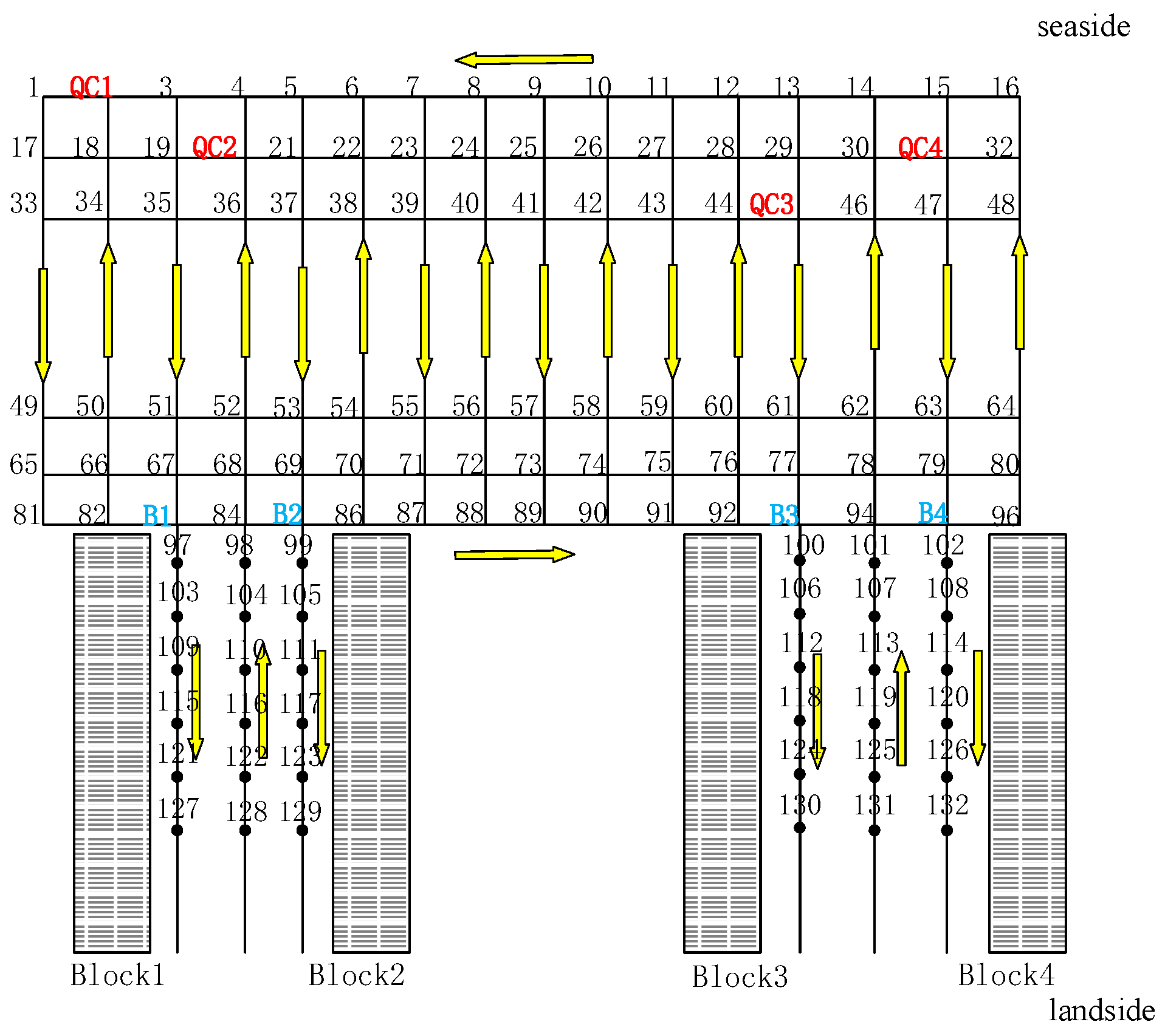
5.1. AGV Path Network

The navigation and positioning of AGVs in the automated container terminal is based on the magnetic nails buried underground [11] as shown in Figure 6. The locations of the magnetic nails are the nodes of the AGV path network.

In Figure 6, different colors denote the work areas of different equipment. QC 1, QC2, QC3 and QC4 represent the work areas of 4 Quay Cranes. There are 132 nodes to simulate the magnetic nails. The nodes for AGVs to enter the yard are B1, B2, B3, and B4. The nodes for AGV to leave the yard are 84 and 94. The yellow arrows represent the directions of AGVs’ travel.

5.2. Parameter Setting

This paper focuses on the unloading mode in a U-shaped automated container terminal. The layout of the terminal is shown in Figure 1. In the horizontal transportation area, the length is 300 m and the width is 120 m. The length of one bay in the storage yard is 20 m, and there are 20 bays in each storage yard area. There are four quay cranes, four blocks, and eight dual-cantilever rail cranes. The AGV speed is 5 m/s and the double-cantilever rail crane speed is 2 m/s. The time for the QC to handle the container to the AGV is 30 s, and the time for the cantilever to handle the container from the AGV to the target bay is 30 s [4,29,30,31]. The algorithm parameters [23,24] are shown in

Table 1. The values of the algorithm parameters.

Algorithm Parameters	Value
$popsiz$	50
$Maxgen$	200
$f_c$	2
$u$	1
$v$	1
$p_c$	0.5
$p_{max}$	0.8
$p_{min}$	0.1

.

$popsiz$$Maxgen$$f_c$$u$$v$$p_c$$p_{max}$$p_{min}$

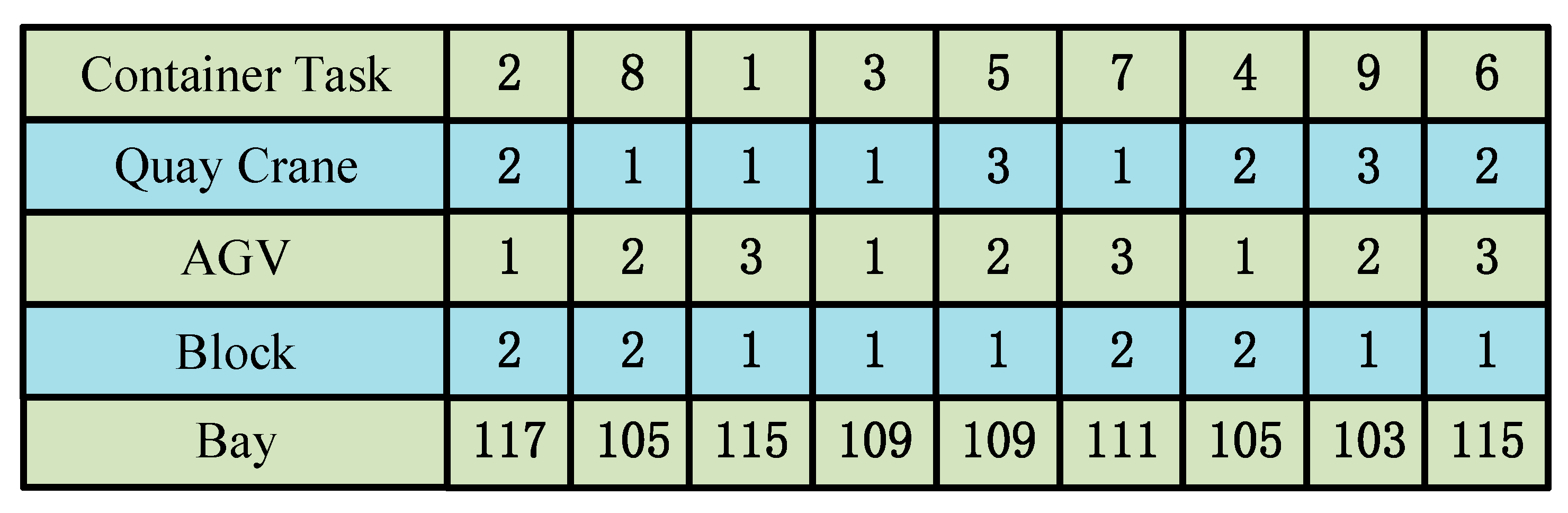
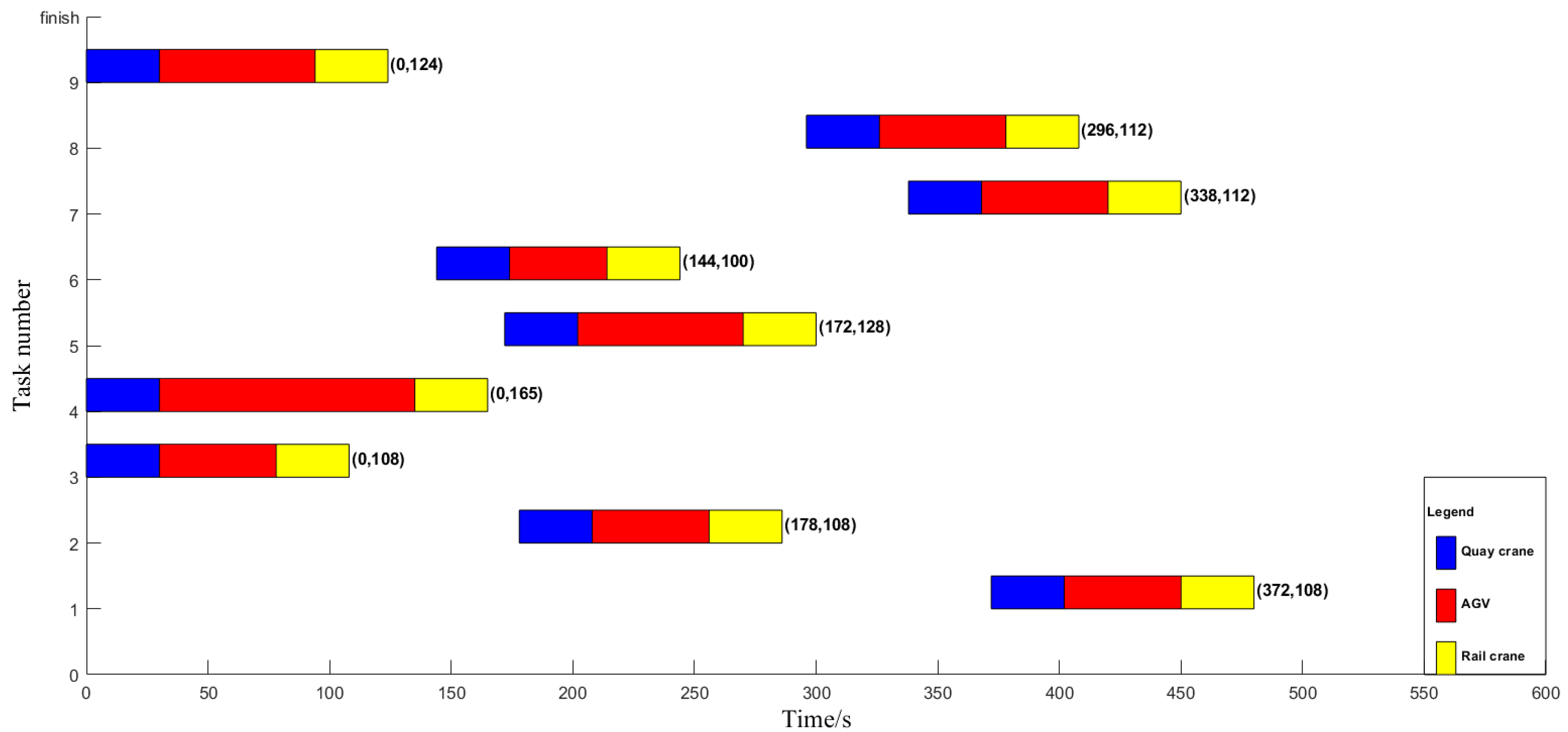
5.3. Results for Small-Sized Problems

There are nine unloading tasks. The starting and ending points of the tasks are known. The specific task allocation is shown in

Table 2. The AGV task allocation.

AGVs	Container Tasks	Starting Points—Ending Points
1	3, 6, 8	QC1-109-QC2-115-QC1-105
2	4, 5, 1	QC2-105-QC3-109-QC1-115
3	9, 2, 7	QC3-103-QC2-117-QC1-111

.

Table 2 shows the task allocation of AGVs. “AGVs” represents the serial numbers of AGVs. “Container tasks” represents the serial numbers of container tasks. “Starting points—Ending points” represents the starting points and the ending points of AGVs. AGV 1 completes three unloading tasks in sequence according to the assignment, and the task numbers are 3, 6, and 8, respectively. The starting and ending points of task 3 are both QC1-109. The starting and ending points of task 6 are both QC2-115. The starting and ending points of task 8 are both QC1-105. Therefore, the path of AGV 1 is QC1-109-QC2-115-QC1-105.

The integer programming model and the path search method are used to determine the path from the starting point to the ending point. Then, the shortest path is determined according to the path length and the number of turns. According to the AGV task allocation in Table 2, the shortest paths and the optimized alternative paths for AGV 1 are shown in

Table 3. The paths of the AGV 1 to complete the task.

Starting Points—Ending Points	Shortest Path	Best Optimal Alternative Path
QC1-109	QC1-1-17-33-49-65-81-82-B1-97-103-109	QC1-1-17-33-49-50-51-67-B1-97-103-109
109-QC2	109-110-104-98-84-68-52-36-QC2	109-110-104-98-84-B2-86-70-54-38-22-21-QC2
QC2-115	QC2-19-35-51-67-B1-97-103-109-115	QC2-19-18-17-33-49-65-81-82-B1-97-103-109-115
115-QC1	115-116-110-104-98-84-68-52-36-QC2-4-3-QC1	115-116-110-104-98-84-B2-86-70-54-38-22-6-5-4-3-QC1
QC1-105	QC1-1-17-33-49-65-81-82-B1-84-B2-99-105	QC1-1-17-33-49-50-51-52-53-69-B2-99-105

. Similarly, the shortest paths and the optimized alternative paths for AGV 2 and AGV 3 can be obtained.

In order to verify the effectiveness of the AGV path planning method, experiments were carried out on the AGV path network in Figure 6. The task arrangement is shown in Table 2. Table 3 represents the shortest path and best optimal alternative path of AGV 1 obtained by the lower-layer model. According to the real port operation data, the time for the double-cantilever rail crane to unload a container is assumed to be 30 s. According to the path planning of the lower-layer model, the time point when AGV reaches the designated bay of the block can be obtained. Then, the lower-layer model feeds back the arrival time to the upper-layer model to obtain the waiting time between the AGV and the double-cantilever rail crane. Then, the upper-layer model adds the waiting time to gain the completion time of this task. Finally, the completion time of all unloading tasks can be obtained by performing this operation for each task. Figure 7 is the time window distribution of AGV 1 to AGV 3 under the shortest path. There are conflicts on the paths, and the conflict time windows are marked with a green box in Figure 7. The conflict time window data is shown in

Table 4. The time window of conflict links.

Conflict Object	Conflict Link	The Starting Time of Conflict Link/s	The Ending Time of Conflict Link/s
AGV 1—AGV 3	<QC2,19>	156	178
AGV 1—AGV 3	<QC1,1>	316	330
AGV 1—AGV 3	<99,105>	394	398
AGV 2—AGV 3	<QC1,1>	426	350

. The conflict object represents the serial number of the conflicting AGVs. The conflict link represents the conflicting road section. The starting time of the conflict link/s represents the time when AGV conflict starts. The ending time of the conflict link/s represents the time when AGV conflict ends.

When two AGVs conflict, a hybrid policy of a delay and alternative path is adopted. For each conflict, the delay and alternative path policies are adopted, respectively. After comparing the time of the two policies, the policy with a shorter time is selected for adjustment. The results are shown in Figure 8.

By calling the solution results of the lower AGV conflict-free path planning model, the upper task sequence can be optimized repeatedly. The initial task sequence generated by the upper-layer model is shown in Figure 2. After multiple iterations of the solution results of the bi-level model, the optimization task sequence is shown in Figure 9. The unloading time windows are shown in Figure 10. The mark (372,108) after the first time window represents that the unloading time of container task 1 is 372 s, and it takes 108 s to complete the task. The meaning of the marks after other time windows is similar to that of the first time window, and the final completion time is 480 s.

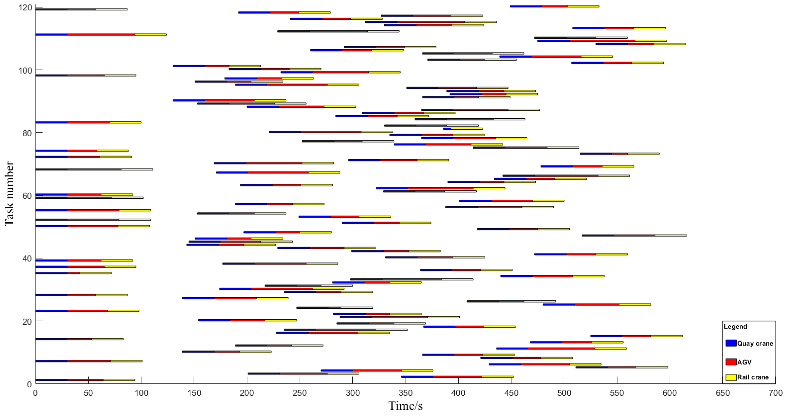
5.4. Results for Large-Sized Problems

In order to verify the effectiveness of the proposed model and algorithm, 15 groups of comparative experiments were carried out using AGA [4], BGA [12], and GSOA. In this paper, each group of instances ran for 30 times, and the target value is the maximum (MAX) and average (AVE), and the running time is the average value. The results are shown in

Table 5. Results of large-sized problems.

			GSOA		AGA		BGA
No.	Containers	AGV	OFV/s MAX/AVE	CPU/s	OFV/s MAX/AVE	CPU/s	OFV/s MAX/AVE	CPU/s
1	40	10	382/363	11	468/447	36	503/486	46
2	80	10	759/725	45	967/950	85	1096/986	76
3	120	10	1120/1080	53	1523/1326	116	1424/1354	126
4	120	20	657/630	31	855/722	135	884/769	154
5	200	20	1089/1034	54	1312/1155	385	1326/1203	425
6	200	50	555/535	67	967/823	399	1066/862	362
7	400	20	1923/1813	329	2551/2336	497	2352/2246	457
8	400	40	1023/962	148	1599/1356	451	1597/1356	489
9	640	20	3117/2930	301	3824/3561	556	3923/3653	582
10	640	40	1593/1501	271	2014/1855	550	1926/1795	586
11	800	40	2007/1873	292	2932/2634	507	2964/2862	487
12	1200	30	3925/3671	327	4725/4423	794	4723/4536	724
13	1200	40	2994/2779	346	3764/3658	780	3961/3782	715
14	2000	40	4806/4558	696	6547/6179	1305	6648/6324	1154
15	2000	50	3952/3709	693	5779/5476	1653	5992/5859	1597

.

It can be seen from the experimental results in Table 5 that:

(1)

In the solving process of GSOA, the hybrid policy of the delay and alternative path can stably obtain the approximately optimal solution of large-sized problems. From examples 13 and 15 in Table 5, when the number of containers is 1200 and the number of AGVs is 40, the average of the objective function value (OFV) is 2779 s; when the number of AGVs is 50, the average of the objective function value is 3709 s, and the difference between the AVE and the MAX is within the acceptable range, which basically meets the time requirements of automated container terminal operation system scheduling.

(2)

As the number of containers increases, the total unloading time of the terminal also increases. With the same number of containers, the increase in the number of AGVs will reduce the total unloading time. Therefore, increasing the number of AGVs to a certain extent can significantly improve the efficiency of handling. Different numbers of tasks and AGVs have significant impacts on the total handling time of the terminal.

Taking 120 container tasks and 20 AGVs as an example, Figure 11 shows the handling time window of the large-sized problem, and the unloading process of the U-shaped automated container terminal is described from three types of time windows: a quay crane handling container, AGV transporting container, and double-cantilever rail crane handling container. In Figure 11, there are 120 three-color line segments representing 120 tasks. Taking task 2 as an example, it is similar to Figure 10. The unloading time of task 2 is 345 s, and 107 s is needed to complete task 2. The other linear time windows are similar to that of task 2. The final completion time is 620 s. From Figure 11, the hybrid policy is effective, and it can successfully realize integrated scheduling optimization in U-shaped automated container terminals.

To further demonstrate the overall performance comparison of the three algorithms, this paper conducted experiments under the conditions of 200 container tasks and 20 AGVs, as shown in Figure 12a. As can be seen from the Figure 12a, BGA, GSOA, and AGA converge in generation 151, 80, and 122, respectively, and the OFVs are 1155, 1034, and 1203 s, respectively. The convergence efficiency of GSOA is better than the other two algorithms. GSOA converges after 80 iterations, and it also has obvious advantages in its solution quality compared with the other two algorithms. Figure 12b shows the results of the 3 algorithms in 2000 container tasks and 50 AGVs. It can be seen from Figure 12b that GSOA converges when it iterates to about 86 generations, and the OFV is 3709 s. The convergence speed and OFV are obviously better than the other two algorithms, which further verifies the effectiveness of GSOA. From Figure 12a,b, 10× more container tasks are handled while only 2.5× more AGVs are available in the U-shaped automated container terminal. It leads to longer processing times for more container tasks.

In order to compare the performances of the 3 optimization algorithms in the case of 120 container tasks and 20 AGVs, the 3 algorithms are run 10 times, respectively, to obtain the OFVs, CPU running time, and convergent generations, as shown in Figure 13. As can be seen from Figure 13, the OFV and CPU running time of the GSOA in this paper are significantly better than the other two algorithms. Although the convergent generation varies greatly, the result is significantly better than the other two algorithms.

In order to test the stability of the proposed GSOA, this paper considers 30 runs with 200 containers, 20 AGVs, 4 QCs, and 8 dual-cantilever rail cranes, and the parameters are the same each time. Figure 14 shows the result of generation 1–200. Each box represents the variation range of the objective function value in different generations; that is, each box represents the OFVs of the 30 runs in one generation. The central mark is the median of OFVs, the edges of the box are the 25th and 75th percentiles, and the whiskers are the most extreme data points. The data reveal that the OFVs of the algorithm have a wide range in the previous generations. With the superposition of evolutionary generation, the algorithm approaches the approximately optimal solution in each generation. An approximately optimal solution can be found in the 180th generation, and the algorithm gradually converges to stability.

6. Conclusions

In this paper, the unloading mode of the U-shaped automated container terminal was considered. Based on the layout of the terminal, a bi-level programming model was established. The upper-layer model is the integrated scheduling model of quay cranes, AGVs, and double-cantilever rail cranes. The lower-layer model is the AGV conflict-free path planning model. The purpose was to minimize the total handling time and improve the efficiency of the terminal. An improved GSOA was designed to solve the model. The GSOA was compared with AGA and BGA to verify the effectiveness of the proposed model and algorithm through large-sized problems. The proposed method was found to be more effective and reliable than AGA and BGA. We experimented with various numbers of containers equipped with different numbers of AGVs to test the GSOA. This process not only revealed reasonable AGV schemes for different quantities of containers but also proved that GSOA obtains favorable solutions within a reasonable amount of time. According to our experiments, the proposed model is practically applicable to the existing U-shaped automated container terminals and may dramatically improve the efficiency.

Integrated scheduling of U-shaped automated container terminals is a complex and interesting problem. Therefore, it can be further studied in future work. The improvements and future research directions are as follows:

(1)

Integrated optimization of automated container terminals contains many aspects and we will take berths and external trucks into consideration in the future.

(2)

External truck appointment system, carbon emission, and sea rail intermodal transportation can also be considered.

(3)

We may also extend the unloading mode into the loading and unloading mode, and the cooperative scheduling problem of the QC, AGV, and double-cantilever rail crane.

References

1. Zhong, M.; Yang, Y.; Zhou, Y.; Postolache, O. Application of hybrid GA-PSO based on intelligent control fuzzy system in the integrated scheduling in automated container terminal. J. Intell. Fuzzy Syst. 2020, 39, 1525–1538. [Google Scholar] [CrossRef]
2. Li, H.; Peng, J.; Wang, X.; Wan, J. Integrated Resource Assignment and Scheduling Optimization With Limited Critical Equipment Constraints at an Automated Container Terminal. IEEE Trans. Intell. Transp. Syst. 2020, 22, 7607–7618. [Google Scholar] [CrossRef]
3. Chen, X.; He, S.; Zhang, Y.; Tong, L.C.; Shang, P.; Zhou, X. Yard crane and AGV scheduling in automated container terminal: A multi-robot task allocation framework. Transp. Res. Part C Emerg. Technol. 2020, 114, 241–271. [Google Scholar] [CrossRef]
4. Luo, J.; Wu, Y. Scheduling of container-handling equipment during the loading process at an automated container terminal. Comput. Ind. Eng. 2020, 149, 106848. [Google Scholar] [CrossRef]
5. Zhen, L.; Yu, S.; Wang, S.; Sun, Z. Scheduling quay cranes and yard trucks for unloading operations in container ports. Ann. Oper. Res. 2019, 273, 455–478. [Google Scholar] [CrossRef]
6. Roy, D.; de Koster, R. Stochastic modeling of unloading and loading operations at a container terminal using automated lifting vehicles. Eur. J. Oper. Res. 2018, 266, 895–910. [Google Scholar] [CrossRef]
7. Zhao, Q.; Ji, S.; Guo, D.; Du, X.; Wang, H. Research on cooperative scheduling of automated quayside cranes and automatic guided vehicles in automated container terminal. Math. Probl. Eng. 2019, 22, 6574582. [Google Scholar] [CrossRef]
8. Jamrus, T.; Chien, C.F.; Gen, M.; Sethanan, K. Hybrid particle swarm optimization combined with genetic operators for flexible job-shop scheduling under uncertain processing time for semiconductor manufacturing. IEEE Trans. Semicond. Manuf. 2017, 31, 32–41. [Google Scholar] [CrossRef]
9. Ma, X.; Bian, Y.; Gao, F. An improved shuffled frog leaping algorithm for multiload AGV dispatching in automated container terminals. Math. Probl. Eng. 2020, 2020, 1260196. [Google Scholar] [CrossRef]
10. Małopolski, W. A sustainable and conflict-free operation of AGVs in a square topology. Comput. Ind. Eng. 2020, 126, 472–481. [Google Scholar] [CrossRef]
11. Xu, B.; Jie, D.; Li, J.; Yang, Y.; Wen, F.; Song, H. Integrated scheduling optimization of U-shaped automated container terminal under loading and unloading mode. Comput. Ind. Eng. 2021, 162, 107695. [Google Scholar] [CrossRef]
12. Yang, Y.; Zhong, M.; Dessouky, Y.; Postolache, O. An integrated scheduling method for AGV routing in automated container terminals. Comput. Ind. Eng. 2018, 126, 482–493. [Google Scholar] [CrossRef]
13. Murakami, K. Time-space network model and MILP formulation of the conflict-free routing problem of a capacitated AGV system. Comput. Ind. Eng. 2020, 141, 106270. [Google Scholar] [CrossRef]
14. Zhong, M.; Yang, Y.; Dessouky, Y.; Postolache, O. Multi-AGV scheduling for conflict-free path planning in automated container terminals. Comput. Ind. Eng. 2020, 142, 371–382. [Google Scholar] [CrossRef]
15. Eglynas, T.; Jakovlev, S.; Jankunas, V.; Didziokas, R.; Januteniene, J.; Drungilas, D.; Jusis, M.; Pocevicius, E.; Bogdevicius, M.; Andziulis, A. Evaluation of the energy consumption of container diesel trucks in a container terminal: A case study at Klaipeda port. Sci. Prog. 2021, 104, 00368504211035596. [Google Scholar] [CrossRef]
16. Yue, L.; Fan, H.; Ma, M. Optimizing configuration and scheduling of double 40 ft dual-trolley quay cranes and AGVs for improving container terminal services. J. Clean. Prod. 2021, 292, 126019. [Google Scholar] [CrossRef]
17. Zhang, Q.; Hu, W.; Duan, J.; Qin, J. Cooperative Scheduling of AGV and ASC in Automation Container Terminal Relay Operation Mode. Math. Probl. Eng. 2021, 2021, 5764012. [Google Scholar] [CrossRef]
18. Jonker, T.; Duinkerken, M.B.; Yorke-Smith, N.; de Waal, A.; Negenborn, R.R. Coordinated optimization of equipment operations in a container terminal. Flex. Serv. Manuf. J. 2021, 33, 281–311. [Google Scholar] [CrossRef]
19. Li, X.; Peng, Y.; Huang, J.; Wang, W.; Song, X. Simulation study on terminal layout in automated container terminals from efficiency, economic and environment perspectives. Ocean Coast. Manag. 2021, 213, 105882. [Google Scholar] [CrossRef]
20. Li, J.; Yang, J.; Xu, B.; Yang, Y.; Wen, F.; Song, H. Hybrid Scheduling for Multi-Equipment at U-Shape Trafficked Automated Terminal Based on Chaos Particle Swarm Optimization. J. Mar. Sci. Eng. 2021, 9, 1080. [Google Scholar] [CrossRef]
21. Guo, K.; Zhu, J.; Shen, L. An Improved Acceleration Method Based on Multi-Agent System for AGVs Conflict-Free Path Planning in Automated Terminals. IEEE Access 2020, 9, 3326–3338. [Google Scholar] [CrossRef]
22. Zhong, M.; Yang, Y.; Sun, S.; Zhou, Y.; Postolache, O.; Ge, Y.E. Priority-based speed control strategy for automated guided vehicle path planning in automated container terminals. Trans. Inst. Meas. Control 2020, 42, 3079–3090. [Google Scholar] [CrossRef]
23. Xin, J.; Negenborn, R.R.; Lodewijks, G. Energy-aware control for automated container terminals using integrated flow shop scheduling and optimal control. Transp. Res. Part C Emerg. Technol. 2014, 44, 214–230. [Google Scholar] [CrossRef]
24. Dhiman, G.; Kumar, V. Seagull optimization algorithm: Theory and its applications for large-scale industrial engineering problems. Knowl. Based Syst. 2019, 165, 169–196. [Google Scholar] [CrossRef]
25. Oliva, D.; Abd Elaziz, M.; Elsheikh, A.H.; Ewees, A.A. A review on meta-heuristics methods for estimating parameters of solar cells. J. Power Sources 2019, 435, 126683. [Google Scholar] [CrossRef]
26. Chen, X.; Yu, K. Hybridizing cuckoo search algorithm with biogeography-based optimization for estimating photovoltaic model parameters. Sol. Energy 2019, 180, 192–206. [Google Scholar] [CrossRef]
27. Long, W.; Cai, S.; Jiao, J.; Xu, M.; Wu, T. A new hybrid algorithm based on grey wolf optimizer and cuckoo search for parameter extraction of solar photovoltaic models. Energy Convers. Manag. 2020, 203, 112243. [Google Scholar] [CrossRef]
28. Xu, B.W.; Liu, X.Y.; Yang, Y.S. Multi-constrained scheduling model and algorithm for truck appointment system considering morning and evening peak periods. Comput. Integr. Manuf. Syst. 2020, 26, 2851–2863. [Google Scholar]
29. Yu, D.; Li, D.; Sha, M.; Zhang, D. Carbon-efficient deployment of electric rubber-tyred gantry cranes in container terminals with workload uncertainty. Eur. J. Oper. Res. 2019, 275, 552–569. [Google Scholar] [CrossRef]
30. Su, L.L.; Samuel, M.; Chong, Y.S. Self-organizing neural network approach for the single AGV routing problem. Eur. J. Oper. Res. 2000, 121, 124–137. [Google Scholar]
31. Kaveshgar, N.; Huynh, N.; Rahimian, S.K. An efficient genetic algorithm for solving the quay crane scheduling problem. Expert Syst. Appl. 2012, 39, 13108–13117. [Google Scholar] [CrossRef]
Figure 1. The layout of a U-shaped automated container terminal.
Jmse 10 01187 g001
Figure 2. Chromosome representation example for tasks.
Jmse 10 01187 g002
Figure 3. An illustration of crossover for the chromosome.
Jmse 10 01187 g003
Figure 4. An illustration of mutation for the chromosome.
Jmse 10 01187 g004
Figure 5. The flowchart of GSOA.
Jmse 10 01187 g005
Figure 6. AGV path network of the U-shaped automated container terminal.
Jmse 10 01187 g006
Figure 7. The time window distribution of AGV 1 to AGV 3.
Jmse 10 01187 g007
Figure 8. The time window distribution of AGV conflict-free path planning.
Jmse 10 01187 g008
Figure 9. The optimization task sequence.
Jmse 10 01187 g009
Figure 10. Time windows of the small-sized problem.
Jmse 10 01187 g010
Figure 11. Time windows of the large-sized problem.
Jmse 10 01187 g011
Figure 12. Experimental results of different algorithms. (a) Performances of different algorithms with 200 container tasks and 20 AGVs. (b) Performances of different algorithms with 2000 container tasks and 50 AGVs.
Jmse 10 01187 g012
Figure 13. Box plot comparisons of the algorithm optimization performances. (a) Comparison of OFV. (b) Comparison of CPU. (c) Comparison of convergent generations.
Jmse 10 01187 g013
Figure 14. Box plot of GSOA in 30 runs.
Jmse 10 01187 g014