
Multiscale Energy Transfers and Conversions of Kuroshio in Luzon Strait and Its Adjacent Regions


Abstract
:1. Introduction
2. Data and Methods
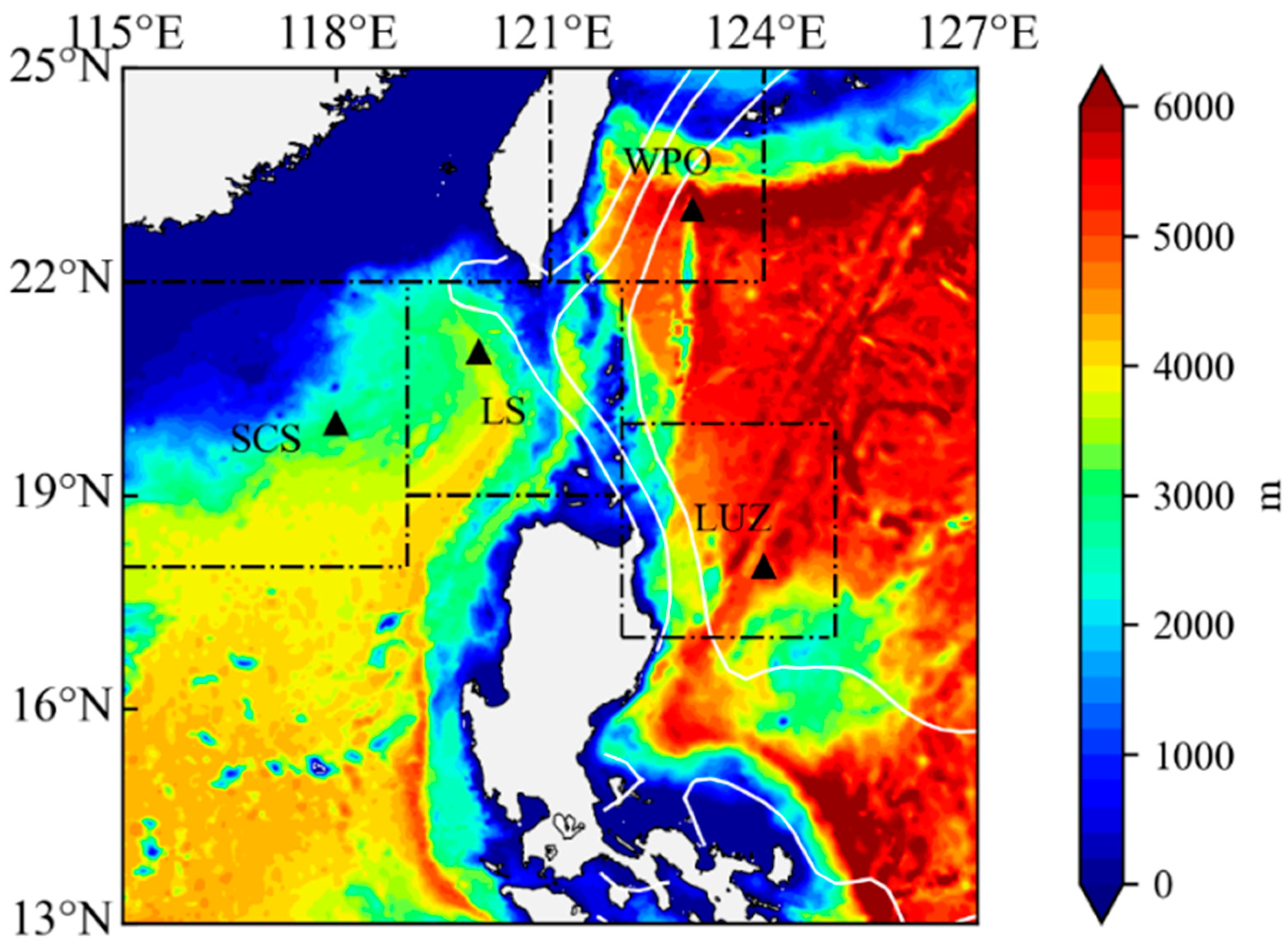
2.1. Data
2.2. Methods
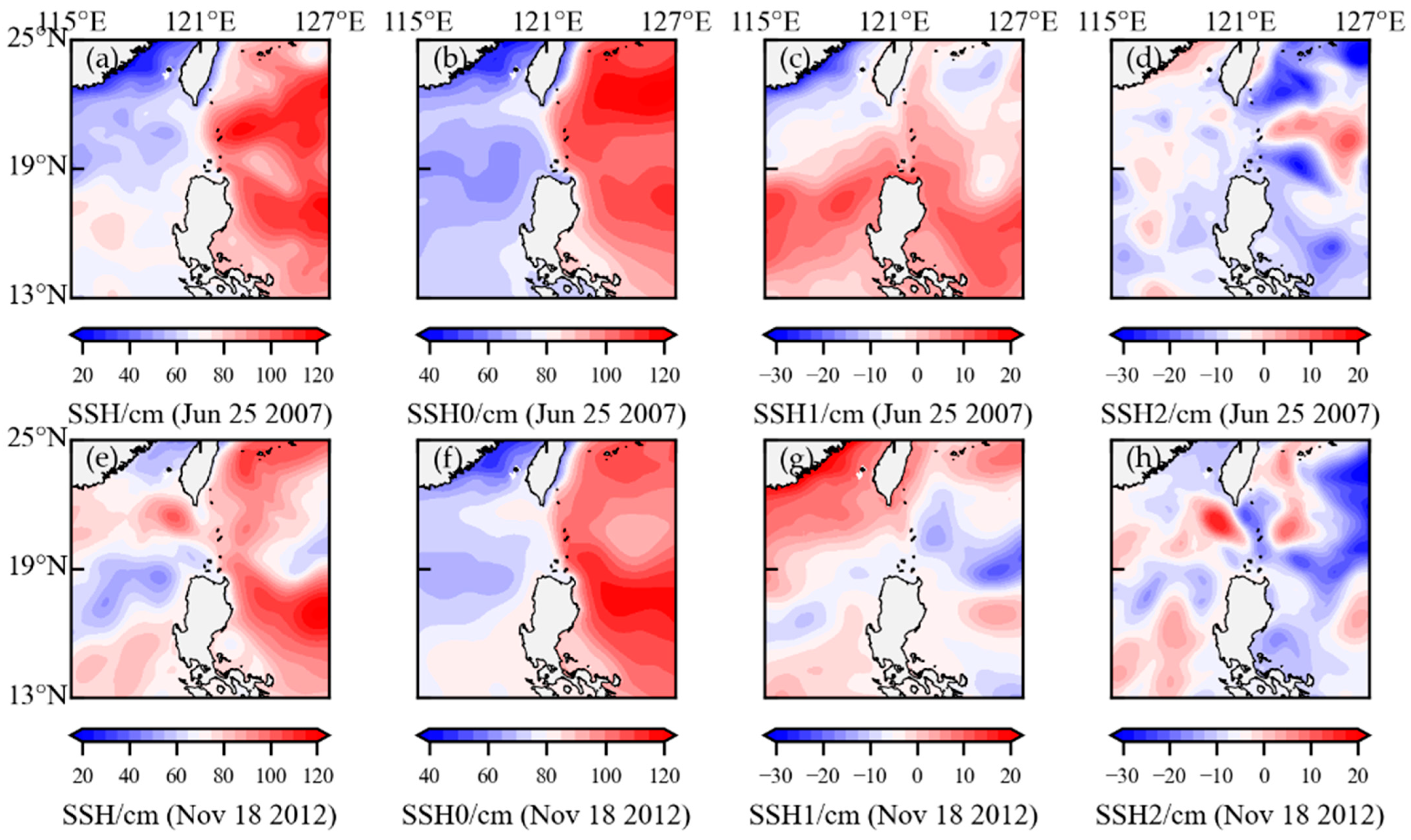
3. Spectral Analysis and Scale Decomposition
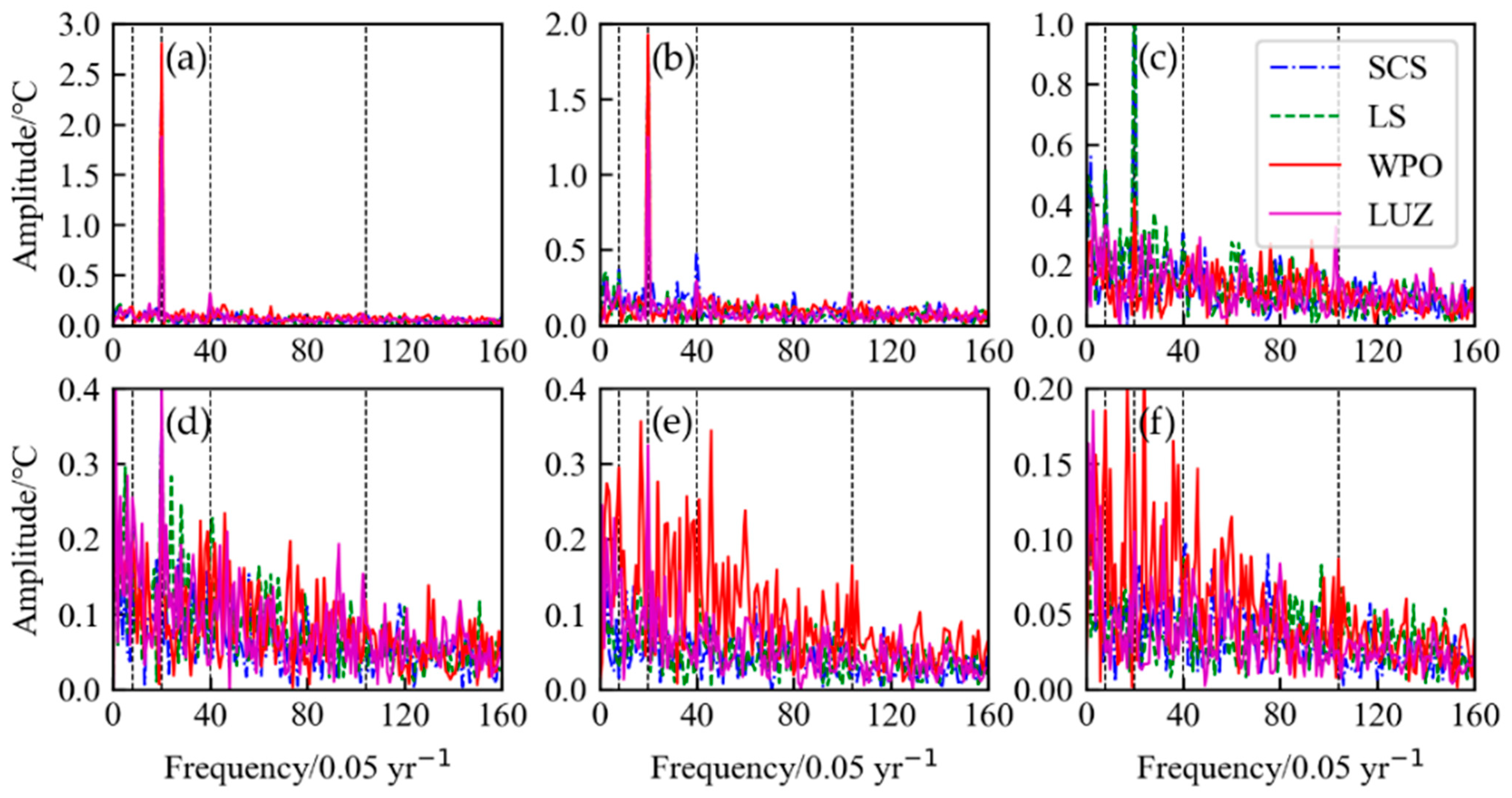
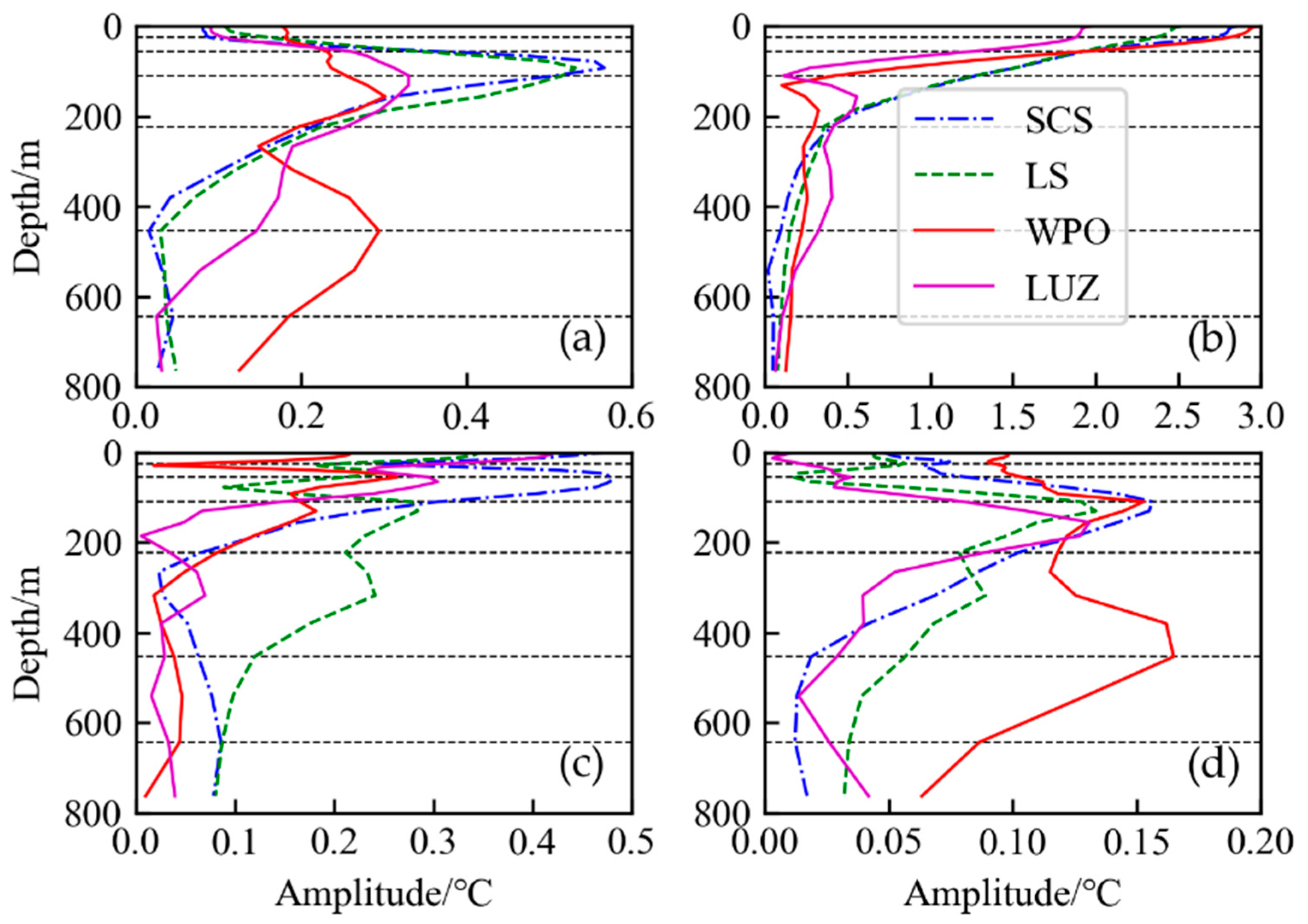
3.1. Spectral Analysis
3.2. Scale Decomposition
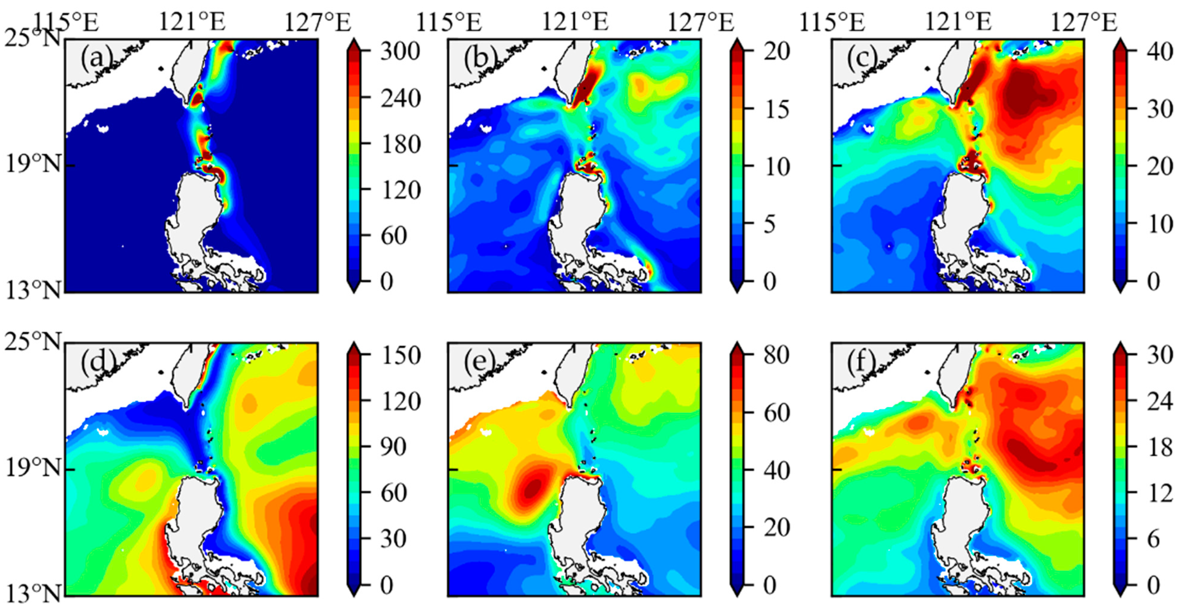
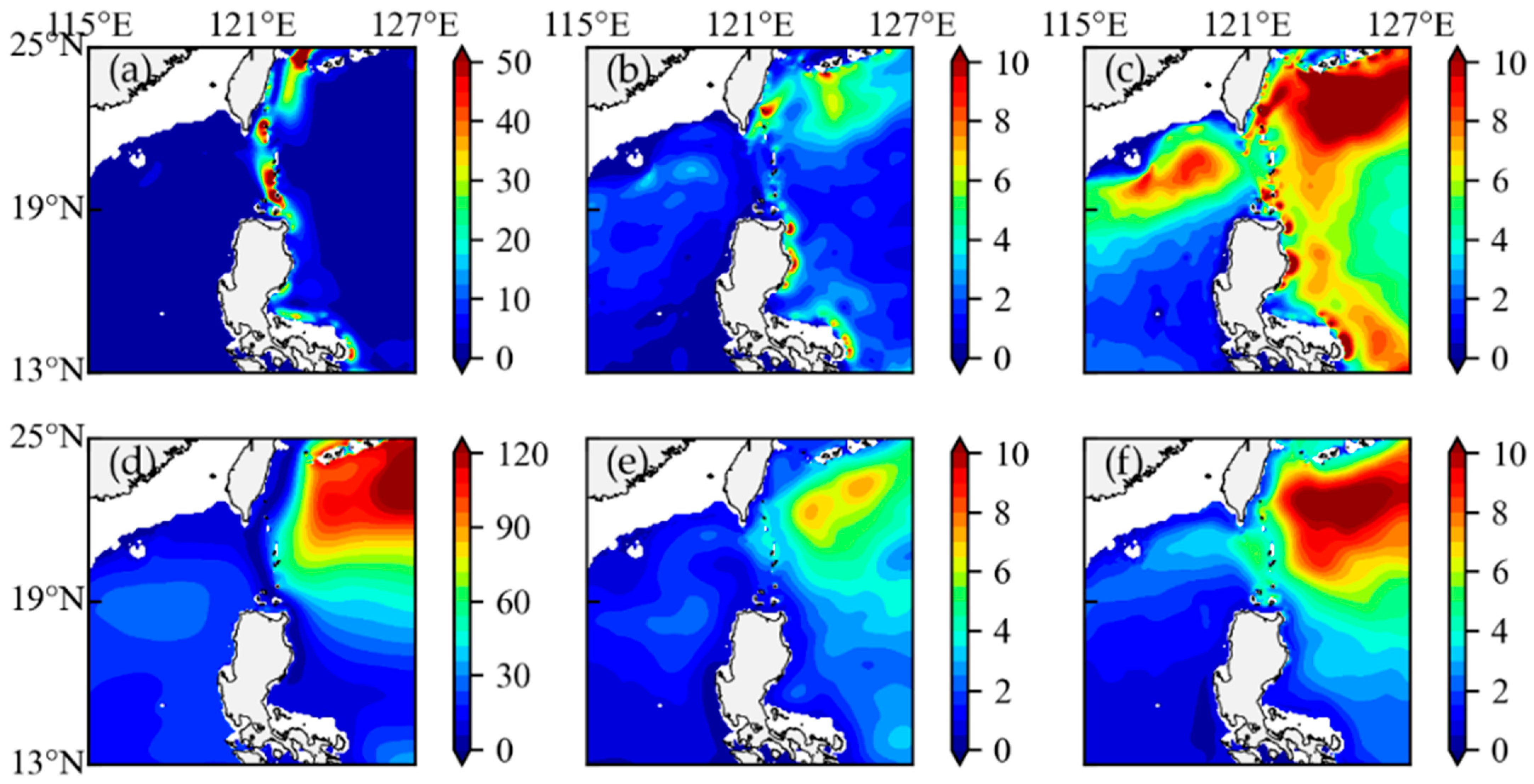
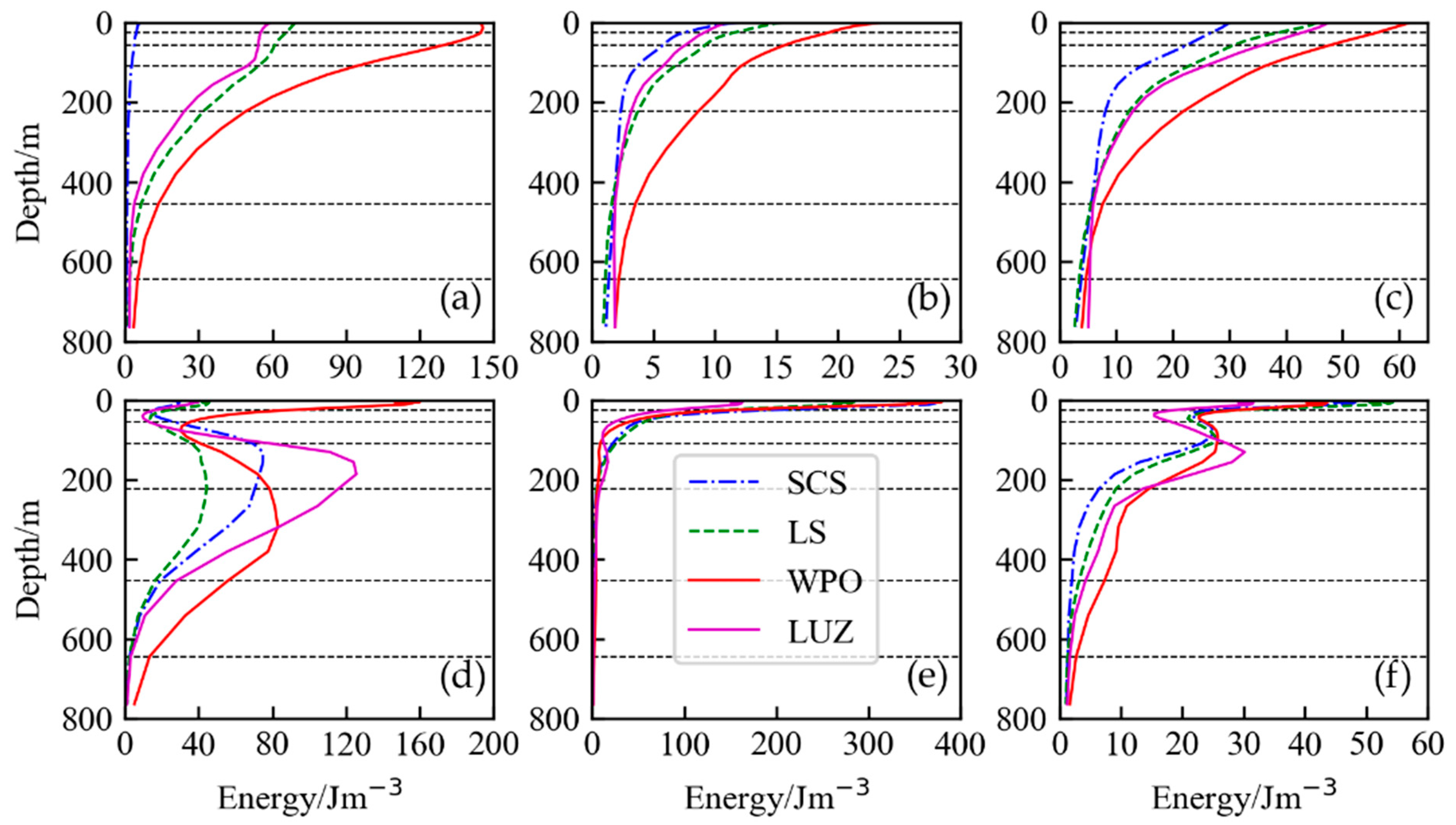
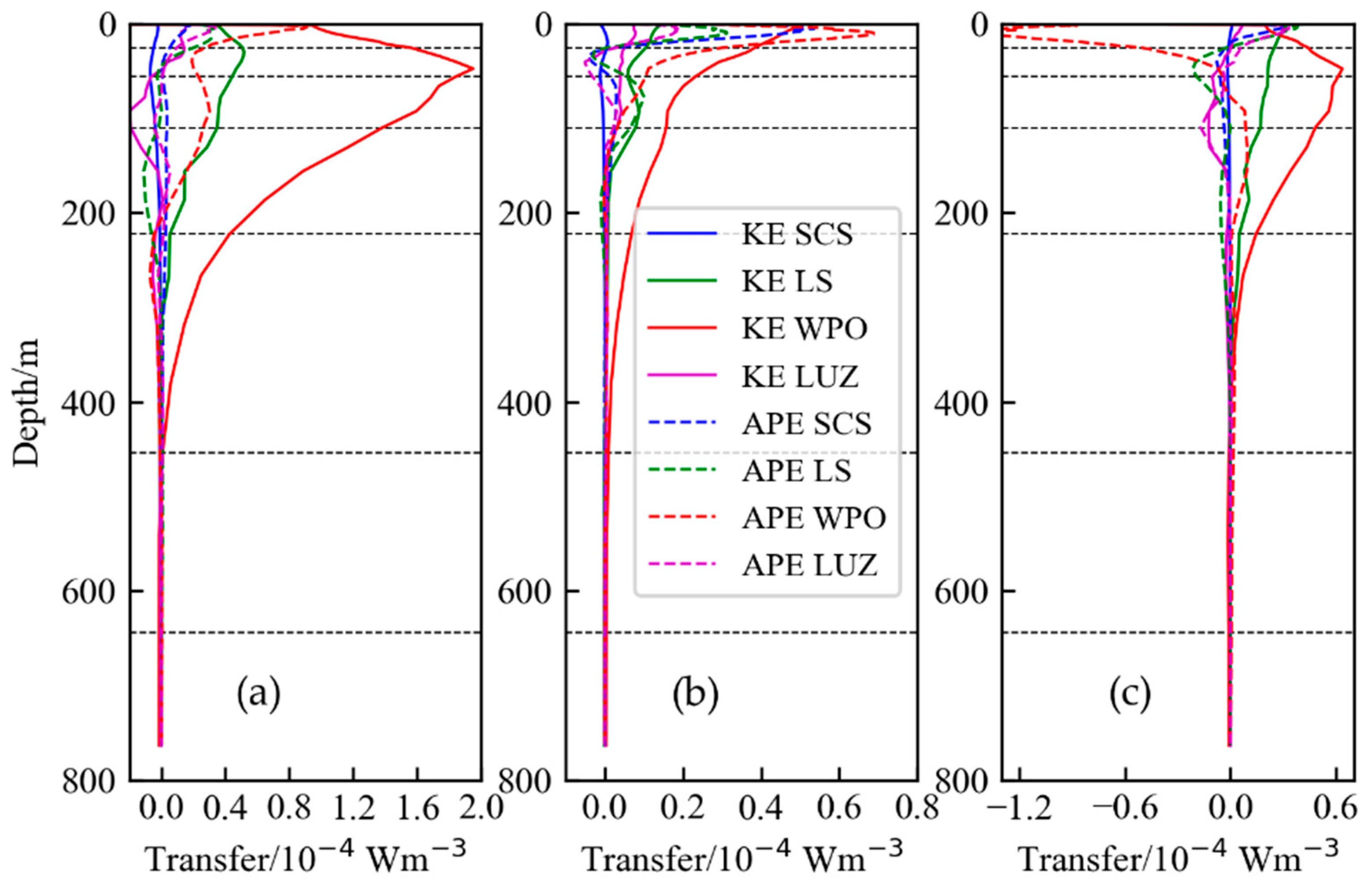
4. Multiscale Energy
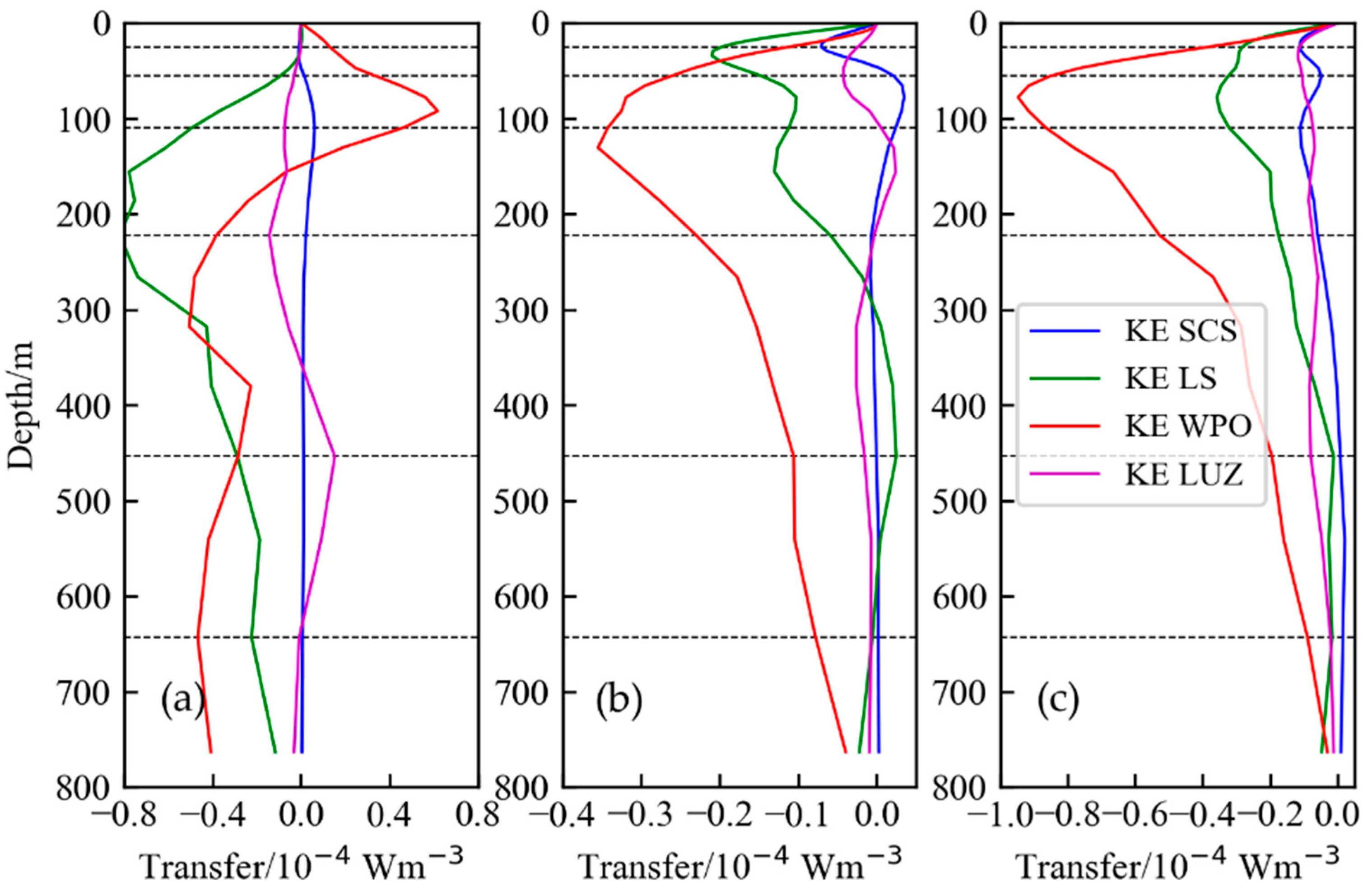
5. Multiscale Interactions
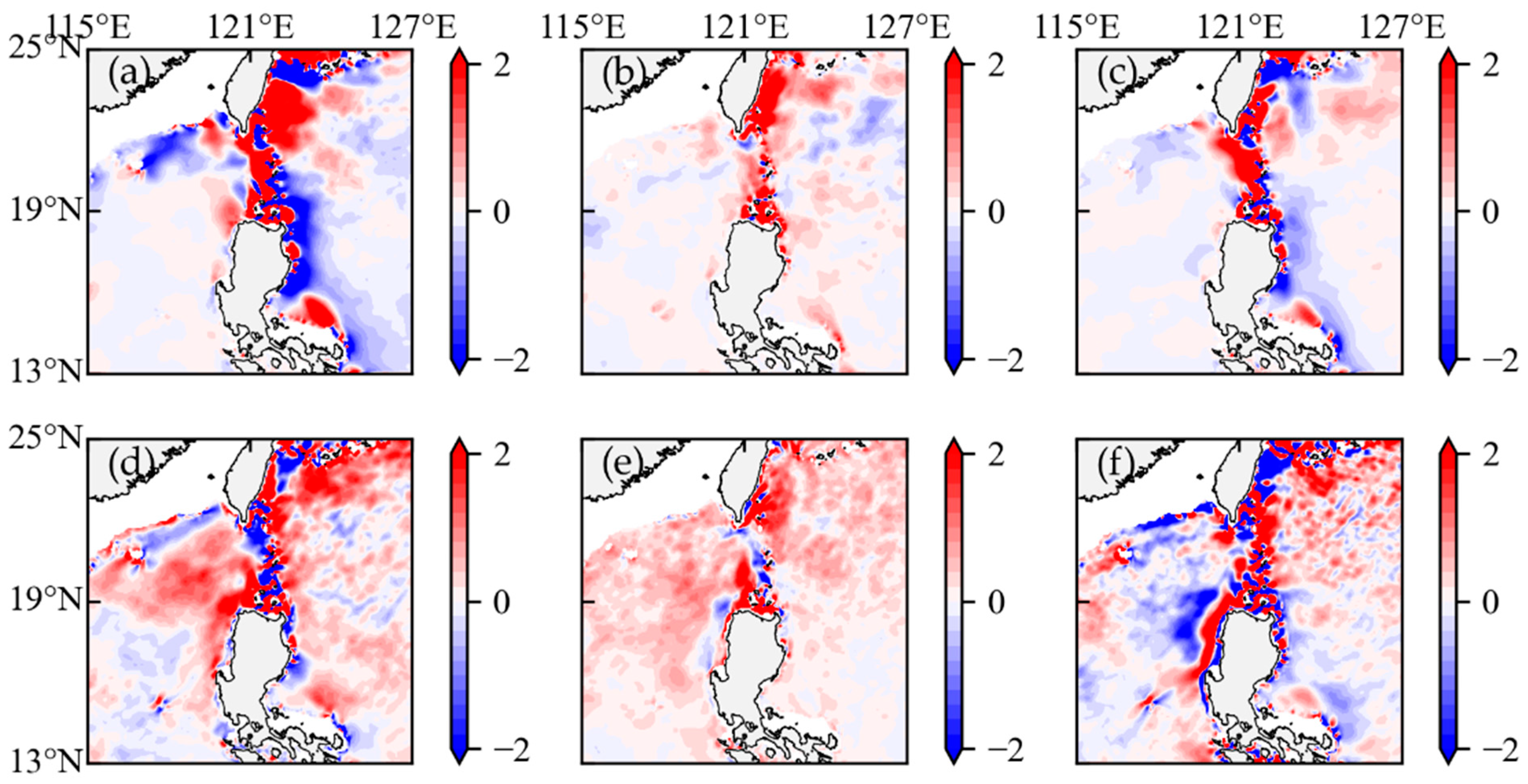
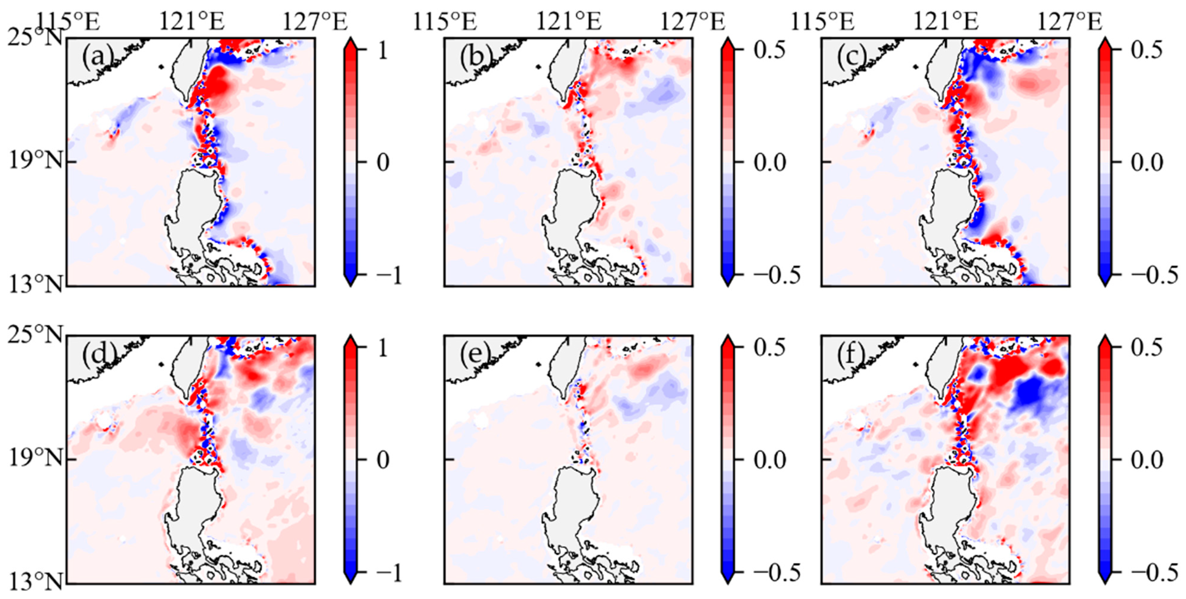
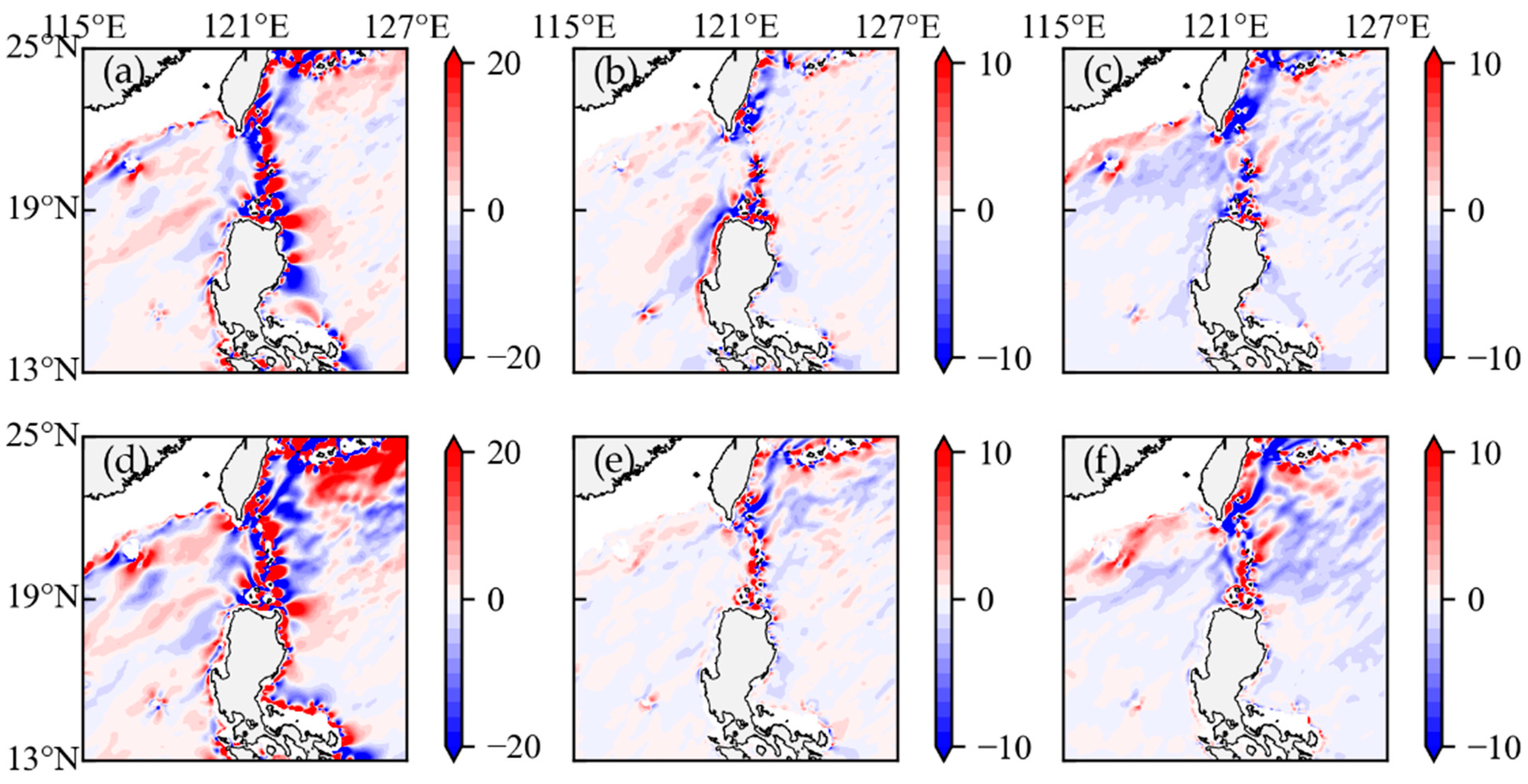
5.1. Climatological-Eddy Interaction
5.2. Seasonal-Eddy Interaction
5.3. Climatological-Seasonal Interaction
5.4. Buoyancy Conversion
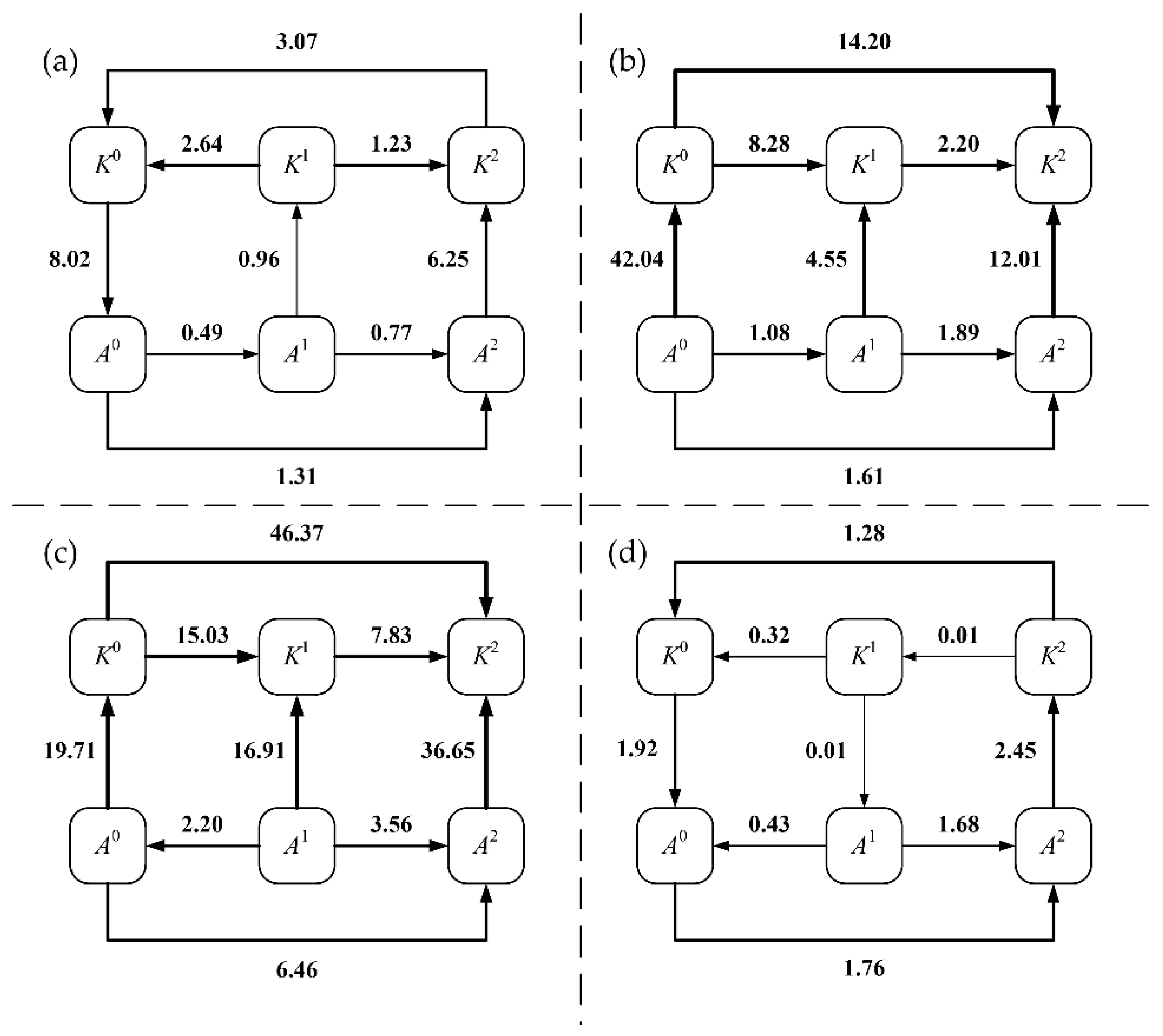
5.5. Energy Pathway and Discussions
6. Conclusions
Author Contributions
Funding
Institutional Review Board Statement
Informed Consent Statement
Data Availability Statement
Acknowledgments
Conflicts of Interest
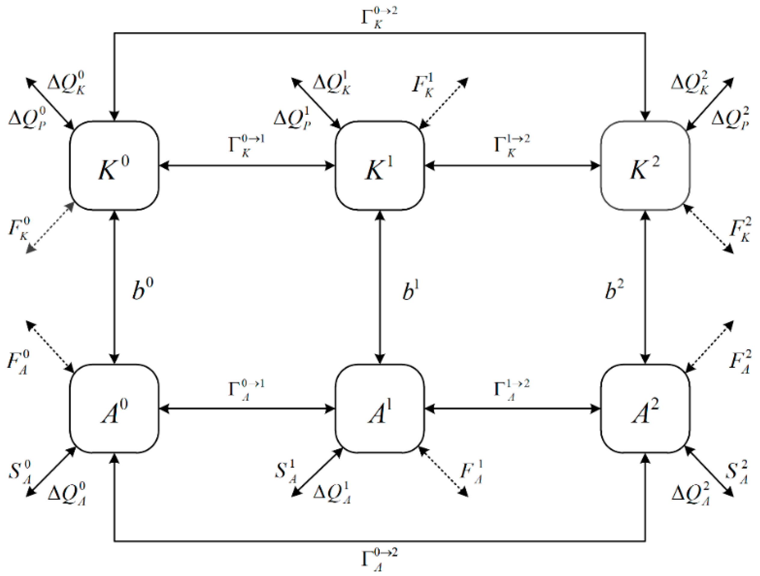
Appendix A. Multiscale Window Transform (MWT)
Appendix B. The Expansion of Canonical Transfer Terms
References
- Yang, S.M.; Xing, J.X.; Sheng, J.Y.; Chen, S.L.; Chen, D.Y. A process study of interactions between a warm eddy and the Kuroshio Current in Luzon Strait: The fate of eddies. J. Mar. Syst. 2019, 194, 66–80. [Google Scholar] [CrossRef]
- Hu, X.M.; Xiong, X.J.; Qiao, F.L.; Guo, B.H.; Lin, X.P. Surface current field and seasonal variability in the Kuroshio and adjacent regions derived from satellite-tracked drifter data. Acta Oceanol. Sin. 2008, 27, 11–29. [Google Scholar]
- Zheng, Q.A.; Tai, C.K.; Hu, J.Y.; Lin, H.Y.; Zhang, R.H.; Su, F.C.; Yang, X.F. Satellite altimeter observations of nonlinear Rossby eddy—Kuroshio interaction at the Luzon Strait. J. Oceanogr. 2011, 67, 365–376. [Google Scholar] [CrossRef]
- Williams, R.G.; Wilson, C.; Hughes, C.W. Ocean and atmosphere storm tracks: The role of eddy vorticity forcing. J. Phys. Oceanogr. 2007, 37, 2267–2289. [Google Scholar] [CrossRef] [Green Version]
- Nan, F.; Xue, H.J.; Yu, F. Kuroshio intrusion into the South China Sea: A review. Prog. Oceanogr. 2015, 137, 314–333. [Google Scholar] [CrossRef] [Green Version]
- Yang, Y.; Liang, X.S. The instabilities and multiscale energetics underlying the mean-interannual-eddy interactions in the Kuroshio Extension region. J. Phys. Oceanogr. 2016, 46, 1477–1494. [Google Scholar] [CrossRef]
- Yang, Y.; Liang, X.S. The intrinsic nonlinear multiscale interactions among the mean flow, low frequency variability and mesoscale eddies in the Kuroshio region. Sci. China Earth Sci. 2019, 62, 595–608. [Google Scholar] [CrossRef]
- Farris, A.; Wimbush, M. Wind-induced Kuroshio intrusion into the South China Sea. J. Oceanogr. 1996, 52, 771–784. [Google Scholar] [CrossRef]
- Sheremet, V.A. Hysteresis of a western boundary current leaping across a gap. J. Phys. Oceanogr. 2001, 31, 1247–1259. [Google Scholar] [CrossRef]
- Zhao, W.; Hou, Y.J.; Qi, P.; Le, K.T.; LI, M.K. The Effects of Monsoons and Connectivity of South China Sea on the Seasonal Variations of Water Exchange in the Luzon Strait. J. Hydrodyn. 2009, 21, 264–270. [Google Scholar] [CrossRef]
- Nan, F.; Xue, H.J.; Chai, F.; Shi, L.; Shi, M.C.; Guo, P.F. Identification of different types of Kuroshio intrusion into the South China Sea. Ocean Dyn. 2011, 61, 1291–1304. [Google Scholar] [CrossRef]
- Tsai, C.J.; Andres, M.; Jan, S.; Mensah, V.; Sanford, T.B.; Lien, R.C.; Lee, C.M. Eddy-Kuroshio interaction processes revealed by mooring observations off Taiwan and Luzon. Geophys. Res. Lett. 2015, 42, 8098–8105. [Google Scholar] [CrossRef] [Green Version]
- Zheng, Q.A.; Ho, C.R.; Xie, L.L.; Li, M.M. A case study of a Kuroshio main path cut-off event and impacts on the South China Sea in fall-winter 2013–2014. Acta Oceanol. Sin. 2019, 38, 12–19. [Google Scholar] [CrossRef]
- Wang, R.; Hou, Y.J.; Liu, Z. Energy sources generation and energy cascades along the Kuroshio east of Taiwan island and the east china sea. J. Mar. Sci. Eng. 2021, 9, 692. [Google Scholar] [CrossRef]
- Yang, Y.; Liang, X.S.; Sasaki, H. Vertical coupling and dynamical source for the intraseasonal variability in the deep Kuroshio Extension. Ocean Dyn. 2021, 71, 1069–1086. [Google Scholar] [CrossRef]
- Chen, Y.C.; Zhai, F.G.; Li, P.L. Decadal Variation of the Kuroshio Intrusion Into the South China Sea During 1992–2016. J. Geophys. Res. Oceans 2020, 125, e2019JC015699. [Google Scholar] [CrossRef]
- Qu, T.D.; Kim, Y.Y.; Yaremchuk, M.; Tuzuka, T.; Ishida, A.; Yamagata, T. Can Luzon Strait transport play a role in conveying the impact of ENSO to the South China Sea? J. Clim. 2004, 17, 3644–3657. [Google Scholar] [CrossRef]
- Kim, Y.Y.; Qu, T.D.; Jensen, T.; Miyama, T.; Mitsudera, H.; Kang, H.W.; Ishida, A. Seasonal and interannual variations of the North Equatorial current bifurcation in a high-resolution OGCM. J. Geophys. Res. Oceans 2004, 109, C03040. [Google Scholar] [CrossRef]
- Yuan, Y.C.; Liao, G.D.; Yang, C.H.; Liu, Z.H.; Chen, H.; Wang, Z.G. Summer Kuroshio Intrusion through the Luzon Strait confirmed from observations and a diagnostic model in summer 2009. Prog. Oceanogr. 2014, 121, 44–59. [Google Scholar] [CrossRef]
- Wu, C.R. Interannual modulation of the Pacific Decadal Oscillation (PDO) on the low-latitude western North Pacific. Prog. Oceanogr. 2013, 110, 49–58. [Google Scholar] [CrossRef]
- Wu, C.R.; Wang, Y.L.; Lin, Y.F.; Chao, S.Y. Intrusion of the Kuroshio into the South and East China Seas. Sci. Rep. 2017, 7, 7895. [Google Scholar] [CrossRef] [PubMed]
- Chang, Y.L.; Oey, L.Y. The Philippines–Taiwan oscillation: Monsoonlike interannual oscillation of the subtropical-Tropical Western North Pacific wind system and its impact on the ocean. J. Climate 2012, 25, 1597–1618. [Google Scholar] [CrossRef]
- Zhang, Z.W.; Zhao, W.; Qiu, B.; Tian, J.W. Anticyclonic eddy sheddings from Kuroshio Loop and the accompanying cyclonic eddy in the northeastern South China Sea. J. Phys. Oceanogr. 2017, 47, 1243–1259. [Google Scholar] [CrossRef] [Green Version]
- Kuo, Y.C.; Chern, C.S.; Zheng, Z.W. Numerical study on the interactions between the Kuroshio current in the Luzon Strait and a mesoscale eddy. Ocean Dyn. 2017, 67, 369–381. [Google Scholar] [CrossRef]
- Qian, S.M.; Wei, H.; Xiao, J.G.; Nie, H.T. Impacts of the Kuroshio intrusion on the two eddies in the northern South China Sea in late spring 2016. Ocean Dyn. 2018, 68, 1695–1709. [Google Scholar] [CrossRef]
- Sun, Z.Y.; Hu, J.Y.; Chen, Z.Z.; Zhu, J.; Yang, L.Q.; Chen, X.R.; Wu, X.W. A strong Kuroshio intrusion into the south china sea and its accompanying cold-core anticyclonic eddy in winter 2020–2021. Remote Sens. 2021, 13, 2645. [Google Scholar] [CrossRef]
- Shen, M.L.; Tseng, Y.H.; Jan, S.; Young, C.C.; Chiou, M.D. Long-term variability of the Kuroshio transport east of Taiwan and the climate it conveys. Prog. Oceanogr. 2014, 121, 60–73. [Google Scholar] [CrossRef]
- Tsui, I.F.; Wu, C.R. Variability analysis of Kuroshio intrusion through Luzon Strait using growing hierarchical self-organizing map. Ocean Dyn. 2012, 62, 1187–1194. [Google Scholar] [CrossRef]
- Hsin, Y.C.; Qiu, B.; Chiang, T.L.; Wu, C.R. Seasonal to interannual variations in the intensity and central position of the surface Kuroshio east of Taiwan. J. Geophys. Res. Oceans 2013, 118, 4305–4316. [Google Scholar] [CrossRef]
- Jan, S.; Mensah, V.; Andres, M.; Chang, M.H.; Yang, Y.J. Eddy-Kuroshio Interactions: Local and Remote Effects. J. Geophys. Res. Oceans 2017, 122, 9744–9764. [Google Scholar] [CrossRef] [Green Version]
- Hou, Y.J.; Liu, Y.H.; Hu, P.; Wang, Z. Nonlinear dynamics of Kuroshio intrusion in the Luzon Strait. Sci. China Earth Sci. 2017, 60, 761–769. [Google Scholar] [CrossRef]
- Cheng, Y.H.; Ho, C.R.; Zheng, Q.A.; Qiu, B.; Hu, J.Y.; Kuo, N.J. Statistical features of eddies approaching the Kuroshio east of Taiwan Island and Luzon Island. J. Oceanogr. 2017, 73, 427–438. [Google Scholar] [CrossRef]
- Jia, Y.L.; Liu, Q.Y.; Liu, W. Primary study of the mechanism of eddy shedding from the Kuroshio bend in Luzon Strait. J. Oceanogr. 2005, 61, 1017–1027. [Google Scholar] [CrossRef]
- Zhao, Y.B.; Liang, X.S.; Gan, J.P. Nonlinear multiscale interactions and internal dynamics underlying a typical eddy-shedding event at Luzon Strait. J. Geophys. Res. Oceans 2016, 121, 3010–3028. [Google Scholar] [CrossRef]
- Feng, B.X.; Liu, H.L.; Lin, P.F. Effects of Kuroshio intrusion optimization on the simulation of mesoscale eddies in the northern South China Sea. Acta Oceanol. Sin. 2020, 39, 12–24. [Google Scholar] [CrossRef]
- Yang, Q.; Liu, H.L.; Lin, P.F.; Li, Y.W. Kuroshio intrusion in the Luzon Strait in an eddy-resolving ocean model and air-sea coupled model. Acta Oceanol. Sin. 2020, 39, 52–68. [Google Scholar] [CrossRef]
- Yin, Y.Q.; Lin, X.P.; He, R.Y.; Hou, Y.J. Impact of mesoscale eddies on Kuroshio intrusion variability northeast of Taiwan. J. Geophys. Res. Oceans 2017, 122, 3021–3040. [Google Scholar] [CrossRef]
- Liang, X.S.; Robinson, A.R. Localized multiscale energy and vorticity analysis I. Fundamentals. Dyn. Atmos. Oceans 2005, 38, 195–230. [Google Scholar] [CrossRef]
- Qiu, B.; Scott, R.B.; Chen, S.M. Length scales of eddy generation and nonlinear evolution of the seasonally modulated South Pacific Subtropical Countercurrent. J. Phys. Oceanogr. 2008, 38, 1515–1528. [Google Scholar] [CrossRef] [Green Version]
- Von Storch, J.S.; Eden, C.; Fast, I.; Haak, H.; Hernández-Deckers, D.; Maier-Reimer, E.; Marotzke, J.; Stammer, D. An estimate of the Lorenz energy cycle for the World Ocean based on the 1/10° STORM/NCEP simulation. J. Phys. Oceanogr. 2012, 42, 2185–2205. [Google Scholar] [CrossRef]
- Chen, R.; Flierl, G.R.; Wunsch, C. A description of local and nonlocal eddy-mean flow interaction in a global eddy-permitting state estimate. J. Phys. Oceanogr. 2014, 44, 2336–2352. [Google Scholar] [CrossRef] [Green Version]
- Liang, X.S.; Robinson, A.R. Localized multi-scale energy and vorticity analysis II. Finite-amplitude instability theory and validation. Dyn. Atmos. Oceans 2007, 44, 51–76. [Google Scholar] [CrossRef]
- Lellouche, J.M.; Le Galloudec, O.; Drévillon, M.; Régnier, C.; Greiner, E.; Garric, G.; Ferry, N.; Desportes, C.; Testut, C.E.; Bricaud, C.; et al. Evaluation of Global Monitoring and Forecasting Systems at Mercator Océan. Ocean Sci. 2013, 9, 57–81. [Google Scholar] [CrossRef] [Green Version]
- Jean-Michel, L.; Eric, G.; Romain, B.B.; Gilles, G.; Angélique, M.; Marie, D.; Clément, B.; Mathieu, H.; Olivier, L.G.; Charly, R.; et al. The Copernicus Global 1/12° Oceanic and Sea Ice GLORYS12 Reanalysis. Front. Earth Sci. 2021, 9, 698876. [Google Scholar] [CrossRef]
- Lorenz, E.N. Available potential energy and the maintenance of the general circulation. Tellus 1955, 7, 157–167. [Google Scholar] [CrossRef] [Green Version]
- Liang, X.S.; Anderson, D.G.M. Multiscale Window Transform. Multiscale Modeling Simul. 2007, 6, 437–467. [Google Scholar] [CrossRef]
- Liang, X.S. Canonical transfer and multiscale energetics for primitive and quasigeostrophic atmospheres. J. Atmos. Sci. 2016, 73, 4439–4468. [Google Scholar] [CrossRef] [Green Version]
- Zhao, Y.H.; Yang, Y.; Liang, X.S.; Zhang, Y.Z. Different mechanisms for the seasonal variations of the mesoscale eddy energy in the South China Sea. Deep-Sea Res. Pt. I 2022, 179, 103677. [Google Scholar] [CrossRef]
- Yang, G.; Wang, F.; Li, Y.L.; Lin, P.F. Mesoscale eddies in the northwestern subtropical Pacific Ocean: Statistical characteristics and three-dimensional structures. J. Geophys. Res. Oceans 2013, 118, 1906–1925. [Google Scholar] [CrossRef]
- Trott, C.B.; Metzger, E.J.; Yu, Z.T. Investigating mesoscale eddy characteristics in the Luzon Strait region using altimetry. Ocean Dyn. 2021, 71, 679–698. [Google Scholar] [CrossRef]
- Chelton, D.B.; Schlax, M.G.; Samelson, R.M. Global observations of nonlinear mesoscale eddies. Prog. Oceanogr. 2011, 91, 167–216. [Google Scholar] [CrossRef]
- Lu, J.Y.; Liu, Q.Y. Gap-leaping Kuroshio and blocking westward-propagating Rossby wave and eddy in the Luzon Strait. J. Geophys. Res. Oceans 2013, 118, 1170–1181. [Google Scholar] [CrossRef]
- Lien, R.C.; Ma, B.; Cheng, Y.H.; Ho, C.R.; Qiu, B.; Lee, C.M.; Chang, M.H. Modulation of Kuroshio transport by mesoscale eddies at the Luzon Strait entrance. J. Geophys. Res. Oceans 2014, 119, 2129–2142. [Google Scholar] [CrossRef]


| Term | Expression | Physical Meaning |
|---|---|---|
| KE advection transport on | ||
| Pressure work of KE on | ||
| Canonical KE transfer to window 1 | ||
| APE advection transport on | ||
| Canonical APE transfer to window | ||
| APE vertical shear on | ||
| Buoyancy conversion on | ||
| —— | Dissipation terms on |
Publisher’s Note: MDPI stays neutral with regard to jurisdictional claims in published maps and institutional affiliations. |
© 2022 by the authors. Licensee MDPI, Basel, Switzerland. This article is an open access article distributed under the terms and conditions of the Creative Commons Attribution (CC BY) license (https://creativecommons.org/licenses/by/4.0/).
Share and Cite
He, Z.; Fu, X.; Zhao, Y.; Jiang, X. Multiscale Energy Transfers and Conversions of Kuroshio in Luzon Strait and Its Adjacent Regions. J. Mar. Sci. Eng. 2022, 10, 975. https://doi.org/10.3390/jmse10070975
He Z, Fu X, Zhao Y, Jiang X. Multiscale Energy Transfers and Conversions of Kuroshio in Luzon Strait and Its Adjacent Regions. Journal of Marine Science and Engineering. 2022; 10(7):975. https://doi.org/10.3390/jmse10070975
Chicago/Turabian StyleHe, Zhongjie, Xiachuan Fu, Yueqi Zhao, and Xuyu Jiang. 2022. "Multiscale Energy Transfers and Conversions of Kuroshio in Luzon Strait and Its Adjacent Regions" Journal of Marine Science and Engineering 10, no. 7: 975. https://doi.org/10.3390/jmse10070975