
Long-Term Monitoring and Change Analysis of Pine Island Ice Shelf Based on Multi-Source Satellite Observations during 1973–2020


Abstract
:1. Introduction
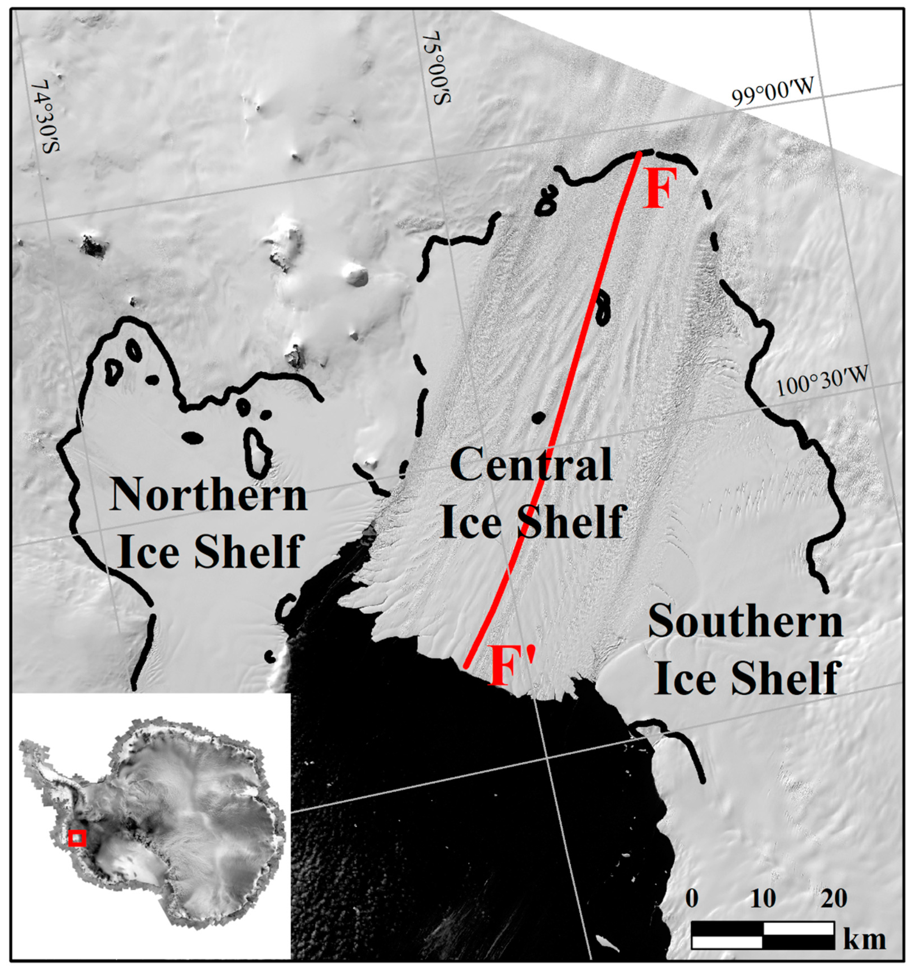
2. Study Area
3. Methodology
3.1. Experimental Data
3.2. Pre-Processing
3.3. Ice Flow Velocity Extraction
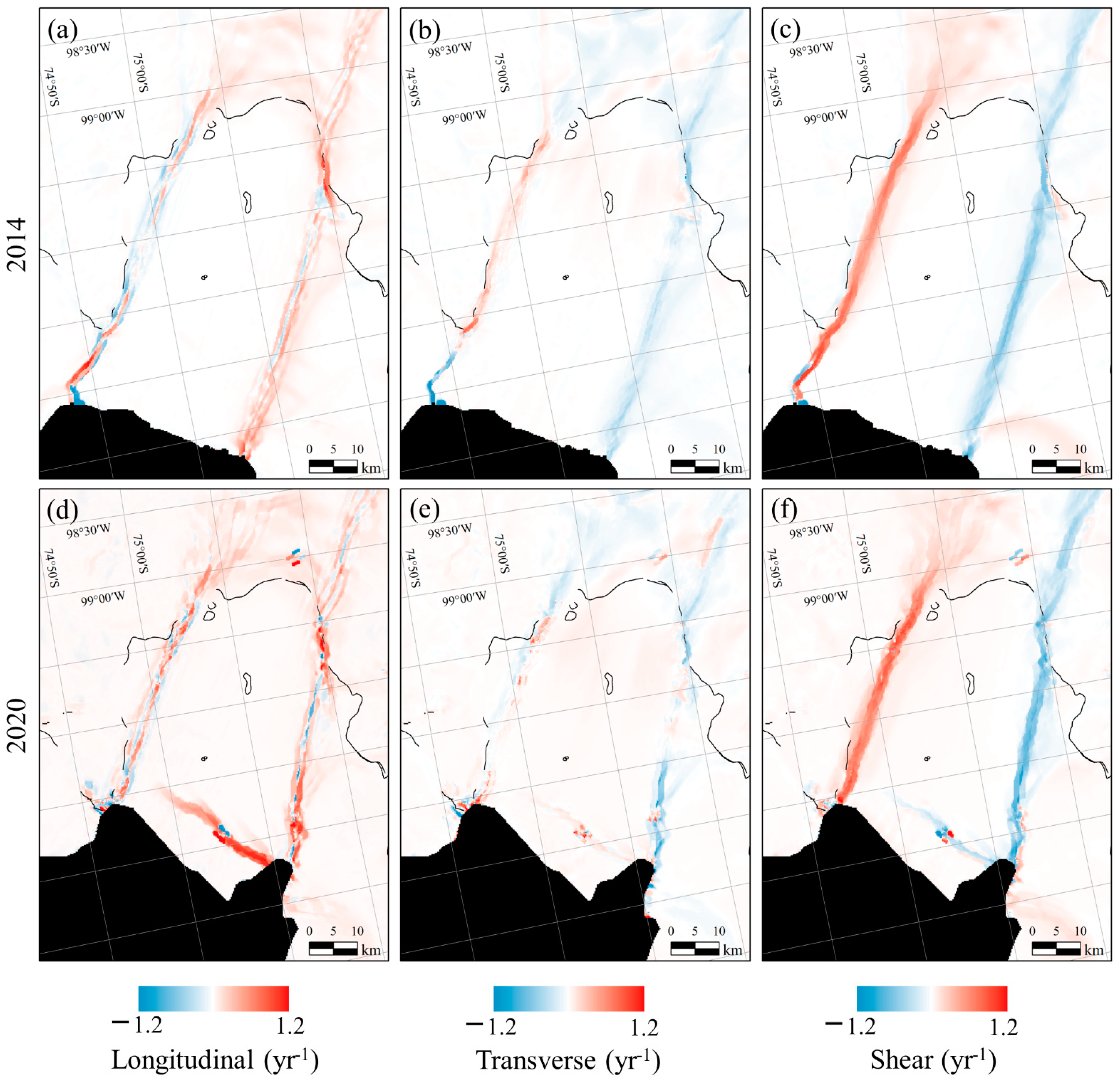
3.4. Surface Strain Rates Retrieval
3.5. Surface Features Extraction
3.6. Ocean Water Temperature Estimation
4. Results
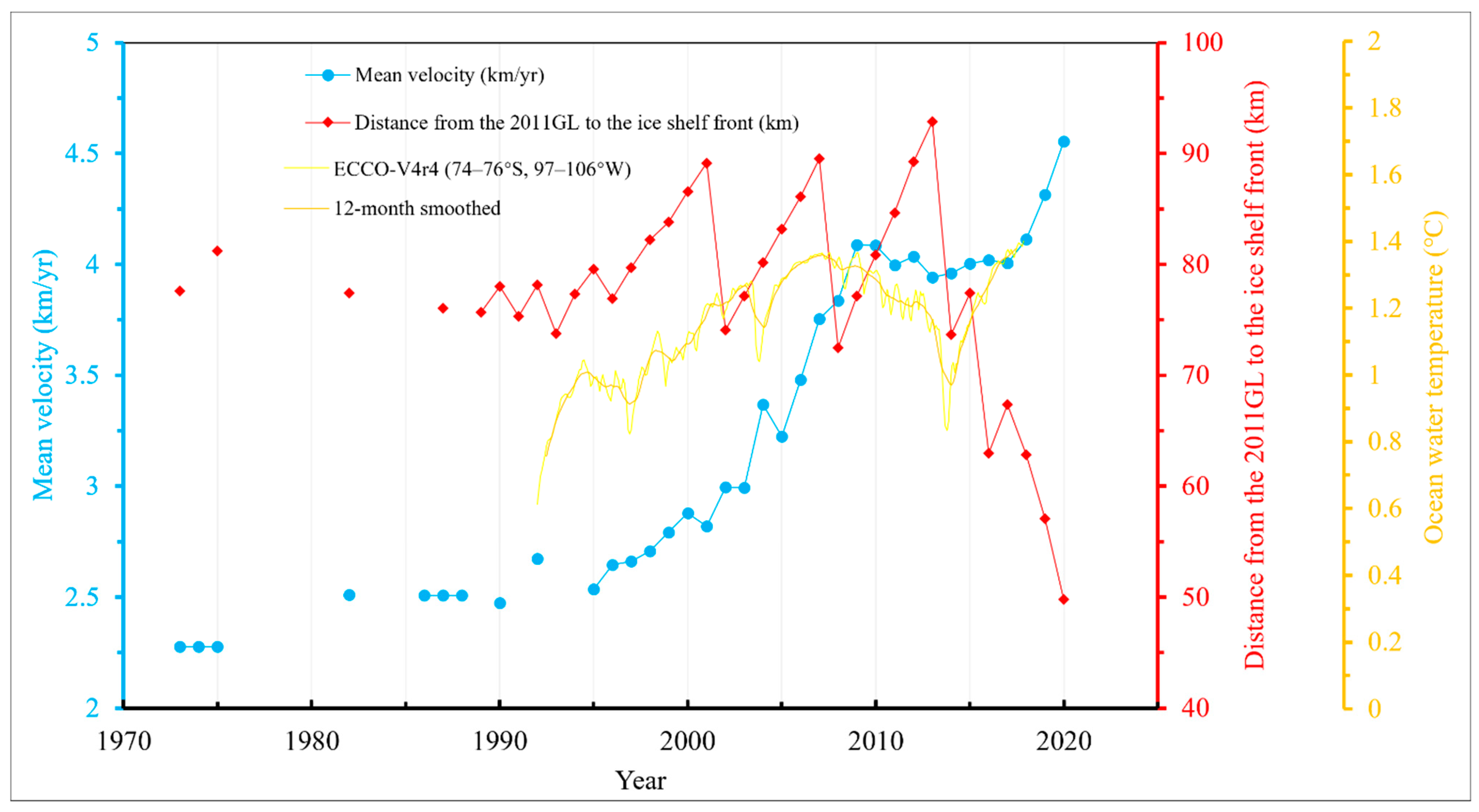
4.1. Interannual Change of Ice Surface Velocities
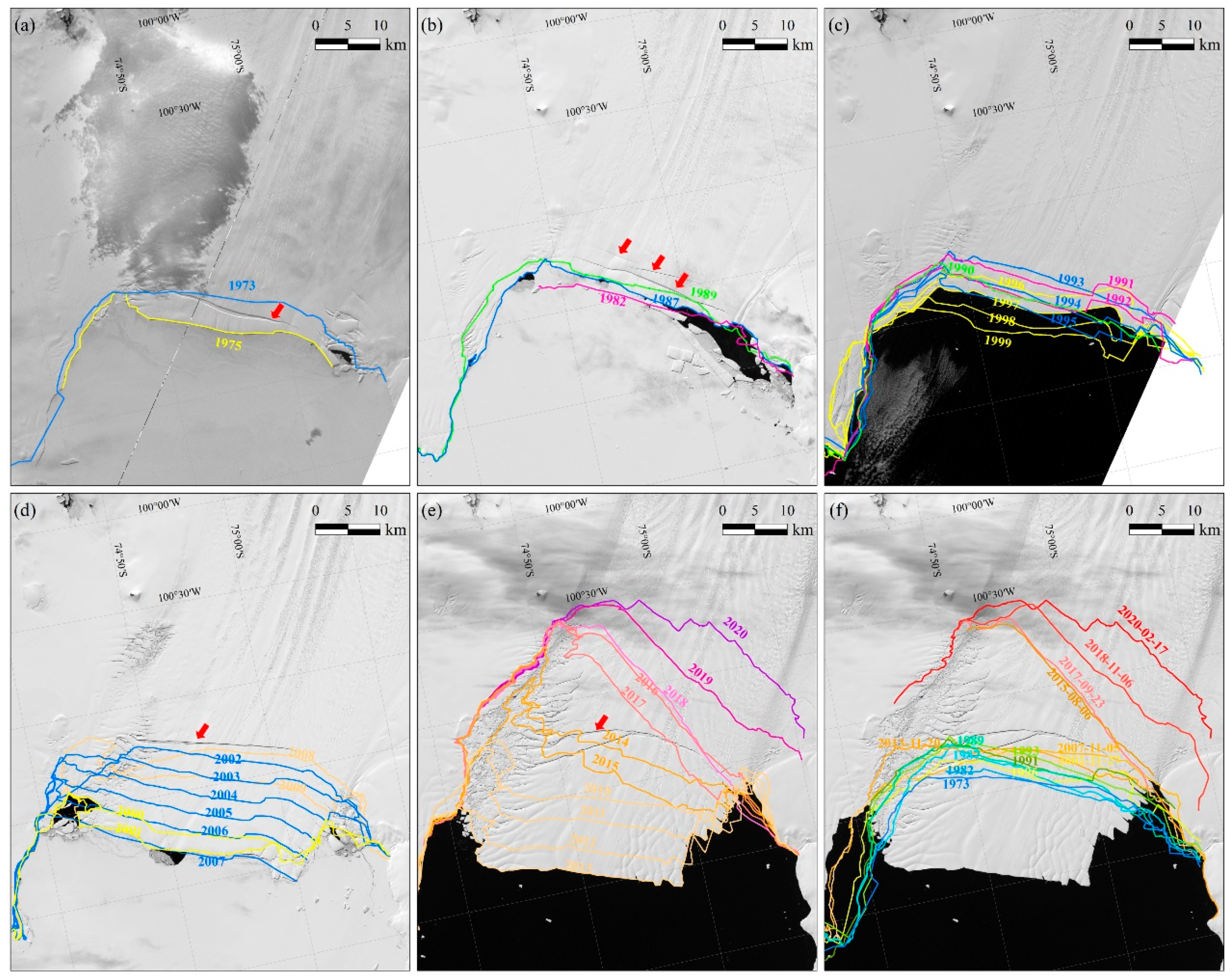
4.2. Ice Shelf Evolution from 1973 to 2020
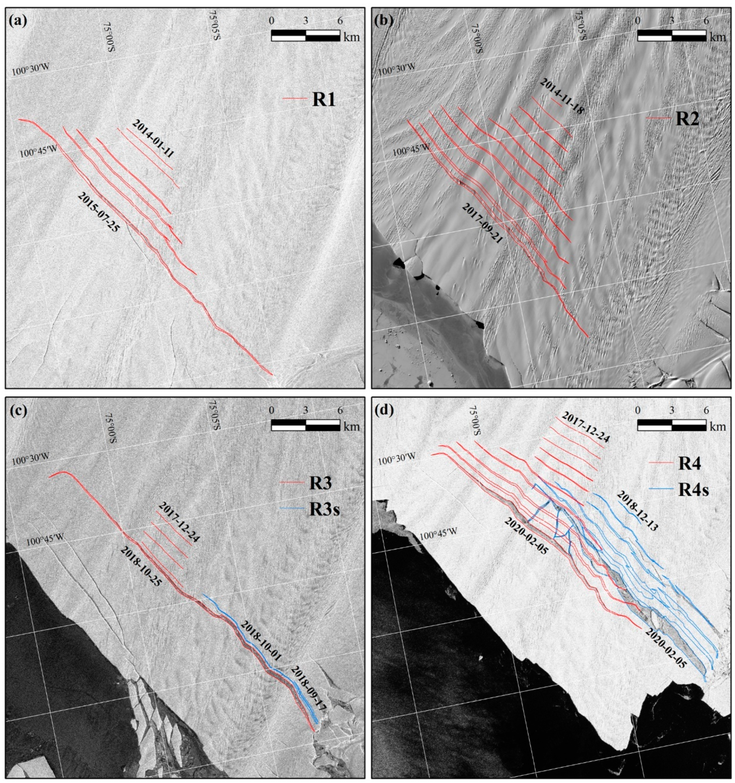
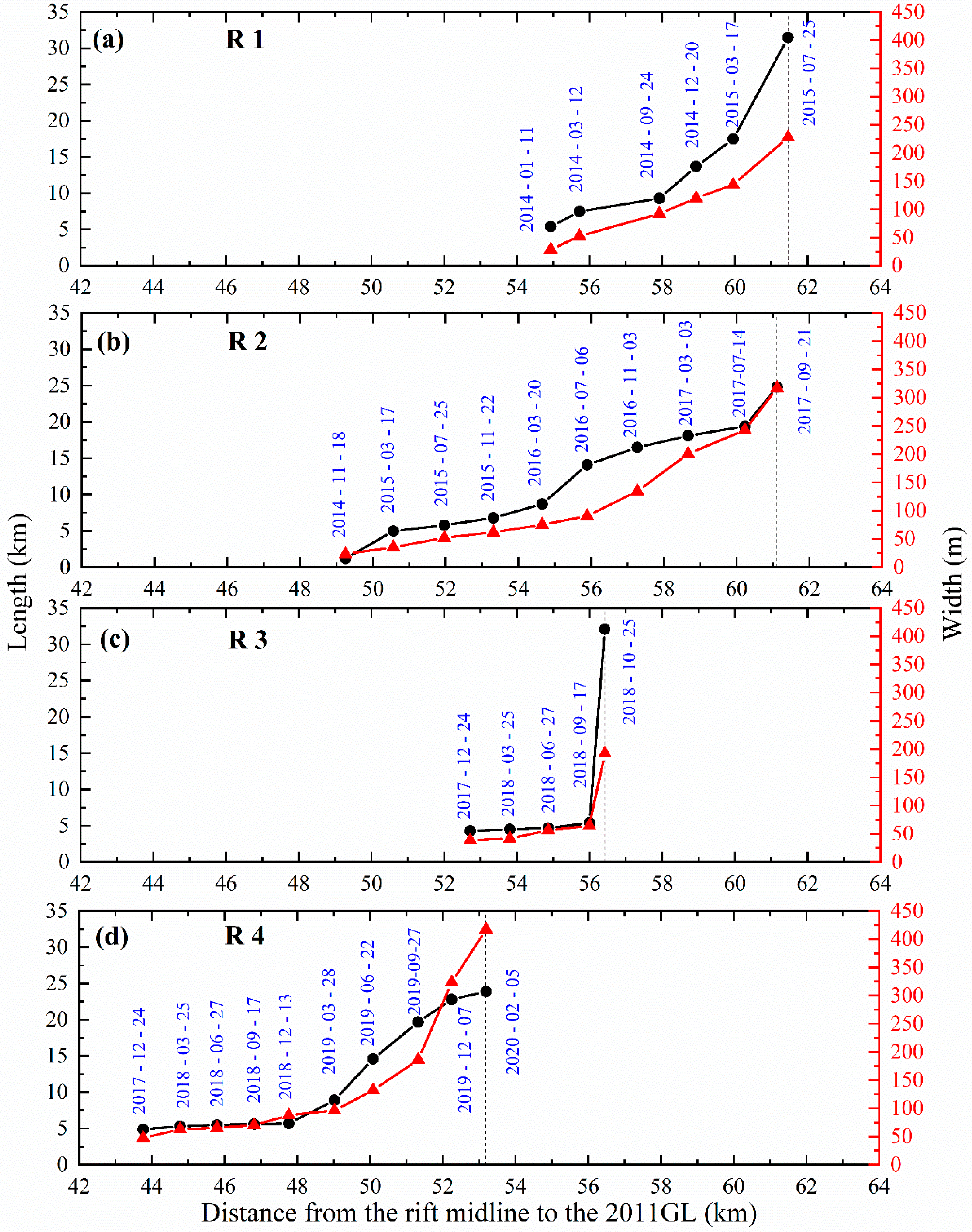
4.3. Rifts Development since 2014
4.4. Rifts Development since 2014
5. Discussion
5.1. Effects of CDW on Ice Flow Velocity and Ice Shelf Disintegration
5.2. The Mechanism of Continuously Formed Rifts and Rapid Retreat
6. Conclusions
Author Contributions
Funding
Institutional Review Board Statement
Informed Consent Statement
Data Availability Statement
Conflicts of Interest
References
- Paolo, F.S.; Fricker, H.A.; Padman, L. Volume Loss from Antarctic Ice Shelves Is Accelerating. Science 2015, 348, 327–331. [Google Scholar] [CrossRef] [PubMed] [Green Version]
- Rignot, E.; Mouginot, J.; Scheuchl, B.; Van Den Broeke, M.; Van Wessem, M.J.; Morlighem, M. Four Decades of Antarctic Ice Sheet Mass Balance from 1979–2017. Proc. Natl. Acad. Sci. USA 2019, 116, 1095–1103. [Google Scholar] [CrossRef] [PubMed] [Green Version]
- Bamber, J.L.; Dawson, G.J. Complex Evolving Patterns of Mass Loss from Antarctica’s Largest Glacier. Nat. Geosci. 2020, 13, 127–131. [Google Scholar] [CrossRef]
- Jacobs, S.S.; Jenkins, A.; Giulivi, C.F.; Dutrieux, P. Stronger Ocean Circulation and Increased Melting under Pine Island Glacier Ice Shelf. Nat. Geosci. 2011, 4, 519–523. [Google Scholar] [CrossRef]
- Bindschadler, R.; Vaughan, D.G.; Vornberger, P. Variability of Basal Melt beneath the Pine Island Glacier Ice Shelf, West Antarctica. J. Glaciol. 2011, 57, 581–595. [Google Scholar] [CrossRef] [Green Version]
- Shean, D.E.; Joughin, I.R.; Dutrieux, P.; Smith, B.E.; Berthier, E. Ice Shelf Basal Melt Rates from a High-Resolution Digital Elevation Model (DEM) Record for Pine Island Glacier, Antarctica. Cryosphere 2019, 13, 2633–2656. [Google Scholar] [CrossRef] [Green Version]
- Scambos, T.A.; Bell, R.E.; Alley, R.B.; Anandakrishnan, S.; Bromwich, D.H.; Brunt, K.; Christianson, K.; Creyts, T.; Das, S.B.; DeConto, R.; et al. How Much, How Fast? A Science Review and Outlook for Research on the Instability of Antarctica’s Thwaites Glacier in the 21st Century. Glob. Planet. Chang. 2017, 153, 16–34. [Google Scholar] [CrossRef]
- Webber, B.G.M.; Heywood, K.J.; Stevens, D.P.; Dutrieux, P.; Abrahamsen, E.P.; Jenkins, A.; Jacobs, S.S.; Ha, H.K.; Lee, S.H.; Kim, T.W. Mechanisms Driving Variability in the Ocean Forcing of Pine Island Glacier. Nat. Commun. 2017, 8, 14507. [Google Scholar] [CrossRef] [Green Version]
- Jenkins, A.; Shoosmith, D.; Dutrieux, P.; Jacobs, S.; Kim, T.W.; Lee, S.H.; Ha, H.K.; Stammerjohn, S. West Antarctic Ice Sheet Retreat in the Amundsen Sea Driven by Decadal Oceanic Variability. Nat. Geosci. 2018, 11, 733–738. [Google Scholar] [CrossRef]
- Mouginot, J.; Scheuch, B.; Rignot, E. Mapping of Ice Motion in Antarctica Using Synthetic-Aperture Radar Data. Remote Sens. 2012, 4, 2753–2767. [Google Scholar] [CrossRef] [Green Version]
- Mouginot, J.; Rignot, E.; Scheuchl, B.; Millan, R. Comprehensive Annual Ice Sheet Velocity Mapping Using Landsat-8, Sentinel-1, and RADARSAT-2 Data. Remote Sens. 2017, 9, 364. [Google Scholar] [CrossRef] [Green Version]
- Gardner, A.S.; Moholdt, G.; Scambos, T.; Fahnstock, M.; Ligtenberg, S.; van den Broeke, M.; Nilsson, J. Increased West Antarctic and Unchanged East Antarctic Ice Discharge over the Last 7 Years. Cryosphere 2018, 12, 521–547. [Google Scholar] [CrossRef] [Green Version]
- Rignot, E.; Vaughan, D.G.; Schmeltz, M.; Dupont, T.; MacAyeal, D. Acceleration of Pine Island and Thwaites Glaciers, West Antarctica. Ann. Glaciol. 2002, 34, 189–194. [Google Scholar] [CrossRef] [Green Version]
- Joughin, I.; Smith, B.E.; Holland, D.M. Sensitivity of 21st Century Sea Level to Ocean-Induced Thinning of Pine Island Glacier, Antarctica. Geophys. Res. Lett. 2010, 37, 1–5. [Google Scholar] [CrossRef]
- Feldmann, J.; Levermann, A. Collapse of the West Antarctic Ice Sheet after Local Destabilization of the Amundsen Basin. Proc. Natl. Acad. Sci. USA 2015, 112, 14191–14196. [Google Scholar] [CrossRef] [Green Version]
- Rignot, E.J. Fast Recession of a West Antarctic Glacier. Science 1998, 281, 549–551. [Google Scholar] [CrossRef] [Green Version]
- Jeong, S.; Howat, I.M.; Bassis, J.N. Accelerated Ice Shelf Rifting and Retreat at Pine Island Glacier, West Antarctica. Geophys. Res. Lett. 2016, 43, 11–720. [Google Scholar] [CrossRef]
- Arndt, J.E.; Larter, R.D.; Friedl, P.; Gohl, K.; Höppner, K.; Afanasyeva, V.; Bickert, T.; Bohaty, S.; Dziadek, R.; Ebermann, B.; et al. Bathymetric Controls on Calving Processes at Pine Island Glacier. Cryosphere 2018, 12, 2039–2050. [Google Scholar] [CrossRef] [Green Version]
- Lhermitte, S.; Sun, S.; Shuman, C.; Wouters, B.; Pattyn, F.; Wuite, J.; Berthier, E.; Nagler, T. Damage Accelerates Ice Shelf Instability and Mass Loss in Amundsen Sea Embayment. Proc. Natl. Acad. Sci. USA 2020, 117, 24735–24741. [Google Scholar] [CrossRef]
- Liu, Y.; Moore, J.C.; Cheng, X.; Gladstone, R.M.; Bassis, J.N.; Liu, H.; Wen, J.; Hui, F. Ocean-Driven Thinning Enhances Iceberg Calving and Retreat of Antarctic Ice Shelves. Proc. Natl. Acad. Sci. USA 2015, 112, 3263–3268. [Google Scholar] [CrossRef] [Green Version]
- Rignot, E.; Mouginot, J.; Scheuchl, B. MEaSUREs Antarctic Grounding Line from Differential Satellite Radar Interferometry, Version 2. Available online: https://doi.org/10.5067/IKBWW4RYHF1Q (accessed on 1 October 2021).
- Rignot, E.; Mouginot, J.; Morlighem, M.; Seroussi, H.; Scheuchl, B. Widespread, Rapid Grounding Line Retreat of Pine Island, Thwaites, Smith, and Kohler Glaciers, West Antarctica, from 1992 to 2011. Geophys. Res. Lett. 2014, 41, 3502–3509. [Google Scholar] [CrossRef] [Green Version]
- Rignot, E.; Mouginot, J.; Scheuchl, B. Antarctic Grounding Line Mapping from Differential Satellite Radar Interferometry. Geophys. Res. Lett. 2011, 38. [Google Scholar] [CrossRef] [Green Version]
- Rignot, E. Ice-Shelf Changes in Pine Island Bay, Antarctica, 1947–2000. J. Glaciol. 2002, 48, 247–256. [Google Scholar] [CrossRef] [Green Version]
- Hughes, T.J. The Weak Underbelly of the West Antarctic Ice Sheet. J. Glaciol. 1981, 27, 518–525. [Google Scholar] [CrossRef] [Green Version]
- Smith, J.A.; Andersen, T.J.; Shortt, M.; Gaffney, A.M.; Truffer, M.; Stanton, T.P.; Bindschadler, R.; Dutrieux, P.; Jenkins, A.; Hillenbrand, C.-D.; et al. Sub-Ice-Shelf Sediments Record History of Twentieth-Century Retreat of Pine Island Glacier. Nature 2017, 541, 77–80. [Google Scholar] [CrossRef]
- Mouginot, J.; Rignot, E.; Scheuchl, B. Sustained Increase in Ice Discharge from the Amundsen Sea Embayment, West Antarctica, from 1973 to 2013. Geophys. Res. Lett. 2014, 41, 1576–1584. [Google Scholar] [CrossRef] [Green Version]
- Liu, H.; Jezek, K.C.; Li, B.; Zhao, Z. Radarsat Antarctic Mapping Project Digital Elevation Model, Version 2. Available online: https://doi.org/10.5067/8JKNEW6BFRVD (accessed on 1 October 2021).
- Bindschadler, R.; Vornberger, P.; Fleming, A.; Fox, A.; Mullins, J.; Binnie, D.; Paulsen, S.J.; Granneman, B.; Gorodetzky, D. The Landsat Image Mosaic of Antarctica. Remote Sens. Environ. 2008, 112, 4214–4226. [Google Scholar] [CrossRef]
- Leprince, S.; Ayoub, F.; Klinger, Y.; Avouac, J.-P. Co-Registration of Optically Sensed Images and Correlation (COSI-Corr): An Operational Methodology for Ground Deformation Measurements. In Proceedings of the 2007 IEEE International Geoscience and Remote Sensing Symposium, Barcelona, Spain, 23–28 July 2007; pp. 1943–1946. [Google Scholar]
- Heid, T.; Kääb, A. Evaluation of Existing Image Matching Methods for Deriving Glacier Surface Displacements Globally from Optical Satellite Imagery. Remote Sens. Environ. 2012, 118, 339–355. [Google Scholar] [CrossRef]
- Fang, L.; Ye, Z.; Su, S.; Kang, J.; Tong, X. Glacier Surface Motion Estimation from SAR Intensity Images Based on Subpixel Gradient Correlation. Sensors 2020, 20, 4396. [Google Scholar] [CrossRef]
- Bindschadler, R.; Vornberger, P.; Blankenship, D.; Scambos, T.; Jacobel, R. Surface Velocity and Mass Balance of Ice Streams D and E, West Antarctica. J. Glaciol. 1996, 42, 461–475. [Google Scholar] [CrossRef] [Green Version]
- Alley, K.E.; Scambos, T.A.; Anderson, R.S.; Rajaram, H.; Pope, A.; Haran, T.M. Continent-Wide Estimates of Antarctic Strain Rates from Landsat 8-Derived Velocity Grids. J. Glaciol. 2018, 64, 321–332. [Google Scholar] [CrossRef] [Green Version]
- Glasser, N.F.; Scambos, T.A. A Structural Glaciological Analysis of the 2002 Larsen B Ice-Shelf Collapse. J. Glaciol. 2008, 54, 3–16. [Google Scholar] [CrossRef] [Green Version]
- MacGregor, J.A.; Catania, G.A.; Markowski, M.S.; Andrews, A.G. Widespread Rifting and Retreat of Ice-Shelf Margins in the Eastern Amundsen Sea Embayment between 1972 and 2011. J. Glaciol. 2012, 58, 458–466. [Google Scholar] [CrossRef] [Green Version]
- Holt, T.O.; Glasser, N.F.; Quincey, D.J.; Siegfried, M.R. Speedup and Fracturing of George VI Ice Shelf, Antarctic Peninsula. Cryosphere 2013, 7, 797–816. [Google Scholar] [CrossRef] [Green Version]
- Forget, G.; Campin, J.-M.; Heimbach, P.; Hill, C.N.; Ponte, R.M.; Wunsch, C. ECCO Version 4: An Integrated Framework for Non-Linear Inverse Modeling and Global Ocean State Estimation. Geosci. Model Dev. 2015, 8, 3071–3104. [Google Scholar] [CrossRef] [Green Version]
- Consortium, E.; Fukumori, I.; Wang, O.; Fenty, I.; Forget, G.; Heimbach, P.; Ponte, R.M. Synopsis of the ECCO Central Production Global Ocean and Sea-Ice State Estimate, Version 4 Release 4 (Version 4 Release 4). Available online: https://zenodo.org/record/4533349 (accessed on 3 May 2021).
- Marshall, J.; Adcroft, A.; Hill, C.; Perelman, L.; Heisey, C. A Finite-Volume, Incompressible Navier Stokes Model for Studies of the Ocean on Parallel Computers. J. Geophys. Res. Ocean. 1997, 102, 5753–5766. [Google Scholar] [CrossRef] [Green Version]
- Rignot, E.; Mouginot, J.; Scheuchl, B. MEaSUREs InSAR-Based Ice Velocity of the Amundsen Sea Embayment, Antarctica, Version 1. Available online: https://doi.org/10.5067/MEASURES/CRYOSPHERE/nsidc-0545.001 (accessed on 1 October 2021).
- Milillo, P.; Rignot, E.; Mouginot, J.; Scheuchl, B.; Morlighem, M.; Li, X.; Salzer, J.T. On the Short-Term Grounding Zone Dynamics of Pine Island Glacier, West Antarctica, Observed with COSMO-SkyMed Interferometric Data. Geophys. Res. Lett. 2017, 44, 436–444. [Google Scholar] [CrossRef] [Green Version]
- Jacobs, S.S.; Hellmer, H.H.; Jenkins, A. Antarctic Ice Sheet Melting in the Southeast Pacific. Geophys. Res. Lett. 1996, 23, 957–960. [Google Scholar] [CrossRef]
- Jenkins, A.; Vaughan, D.G.; Jacobs, S.S.; Hellmer, H.H.; Keys, J.R. Glaciological and Oceanographic Evidence of High Melt Rates beneath Pine Island Glacier, West Antarctica. J. Glaciol. 1997, 43, 114–121. [Google Scholar] [CrossRef]
- Dutrieux, P.; De Rydt, J.; Jenkins, A.; Holland, P.R.; Ha, H.K.; Lee, S.H.; Steig, E.J.; Ding, Q.; Abrahamsen, E.P.; Schröder, M. Strong Sensitivity of Pine Island Ice-Shelf Melting to Climatic Variability. Science 2014, 343, 174–178. [Google Scholar] [CrossRef] [Green Version]
- Arthern, R.J.; Williams, C.R. The Sensitivity of West Antarctica to the Submarine Melting Feedback. Geophys. Res. Lett. 2017, 44, 2352–2359. [Google Scholar] [CrossRef] [Green Version]
- Bassis, J.N.; Fricker, H.A.; Coleman, R.; Minster, J.-B. An Investigation into the Forces That Drive Ice-Shelf Rift Propagation on the Amery Ice Shelf, East Antarctica. J. Glaciol. 2008, 54, 17–27. [Google Scholar] [CrossRef] [Green Version]
- Walker, C.C.; Bassis, J.N.; Fricker, H.A.; Czerwinski, R.J. Structural and Environmental Controls on Antarctic Ice Shelf Rift Propagation Inferred from Satellite Monitoring. J. Geophys. Res. Earth Surf. 2013, 118, 2354–2364. [Google Scholar] [CrossRef]
- Walker, C.C.; Bassis, J.N.; Fricker, H.A.; Czerwinski, R.J. Observations of Interannual and Spatial Variability in Rift Propagation in the Amery Ice Shelf, Antarctica, 2002–2014. J. Glaciol. 2015, 61, 243–252. [Google Scholar] [CrossRef] [Green Version]


| Landsat Series | Sentinel-1A | ERS-1/2 | |
|---|---|---|---|
| Time | 1973–2020 | 2014–2020 | 1992–1999 |
| Repeat cycle | 18-day (Landsat-1/2/3) 16-day (Landsat-4/5/7/8) | 12-day | 35-day |
| Spatial resolution | 60 m (Landsat-1/2/3) 30 m (Landsat-4/5) 15 m (Landsat-7/8) | 20 m | 25 m |
| Quantity | 61 scenes | 6 scenes | 9 scenes |
| Usage | Extraction of ice flow velocity, ice shelf fronts, and rifts. | Extraction of rifts. | Extraction of ice flow velocity, and ice shelf fronts. |
Publisher’s Note: MDPI stays neutral with regard to jurisdictional claims in published maps and institutional affiliations. |
© 2022 by the authors. Licensee MDPI, Basel, Switzerland. This article is an open access article distributed under the terms and conditions of the Creative Commons Attribution (CC BY) license (https://creativecommons.org/licenses/by/4.0/).
Share and Cite
Liu, S.; Su, S.; Cheng, Y.; Tong, X.; Li, R. Long-Term Monitoring and Change Analysis of Pine Island Ice Shelf Based on Multi-Source Satellite Observations during 1973–2020. J. Mar. Sci. Eng. 2022, 10, 976. https://doi.org/10.3390/jmse10070976
Liu S, Su S, Cheng Y, Tong X, Li R. Long-Term Monitoring and Change Analysis of Pine Island Ice Shelf Based on Multi-Source Satellite Observations during 1973–2020. Journal of Marine Science and Engineering. 2022; 10(7):976. https://doi.org/10.3390/jmse10070976
Chicago/Turabian StyleLiu, Shijie, Shu Su, Yuan Cheng, Xiaohua Tong, and Rongxing Li. 2022. "Long-Term Monitoring and Change Analysis of Pine Island Ice Shelf Based on Multi-Source Satellite Observations during 1973–2020" Journal of Marine Science and Engineering 10, no. 7: 976. https://doi.org/10.3390/jmse10070976