Use of State-of-Art Machine Learning Technologies for Forecasting Offshore Wind Speed, Wave and Misalignment to Improve Wind Turbine Performance

Abstract

One of the most promising solutions that stands out to mitigate climate change is floating offshore wind turbines (FOWTs). Although they are very efficient in producing clean energy, the harsh environmental conditions they are subjected to, mainly strong winds and waves, produce structural fatigue and may cause them to lose efficiency. Thus, it is imperative to develop models to facilitate their deployment while maximizing energy production and ensuring the structure’s safety. This work applies machine learning (ML) techniques to obtain predictive models of the most relevant metocean variables involved. Specifically, wind speed, significant wave height, and the misalignment between wind and waves have been analyzed, pre-processed and modeled based on actual data. Linear regression (LR), support vector machines regression (SVR), Gaussian process regression (GPR) and neural network (NN)-based solutions have been applied and compared. The results show that Nonlinear autoregressive with an exogenous input neural network (NARX) is the best algorithm for both wind speed and misalignment forecasting in the time domain (72% accuracy) and GPR for wave height (90.85% accuracy). In conclusion, these models are vital to deploying and installing FOWTs and making them profitable.

1. Introduction

Today, one of the most significant global challenges that society is facing is climate change. As the United Nations Framework Convention on Climate Change [1] stated, governments worldwide must bet on the development, application and diffusion of new technologies that promote the exploitation and use of renewable energies, reducing emissions of greenhouse gases and mitigating global warming. Wind energy is one of the cleanest and most efficient renewable energy sources [2].

In contrast to onshore wind energy and already mature technology [3], offshore wind energy appeared in the last three decades as a promising solution for some of the main disadvantages of on-land wind turbines, such as the visual and acoustic impact, the negative influence on wildlife, and limited locations. In addition, offshore wind energy takes advantage of more stable and robust winds generated in the open sea due to the absence of geographical accidents [4].

There are two main types of offshore wind turbines: bottom fixed and floating. The better-known bottom-fixed one has a high installation cost, as the whole structure is anchored to the seabed, thus requiring shallow waters, and maintenance is also difficult [5]. In addition, the visual impact is not completely removed, and these offshore wind devices are invasive to the abundant wildlife near the coasts. To mitigate some of these issues, the idea of installing offshore wind farms in deeper and farther waters resulted in the design of Floating Offshore Wind Turbines (FOWTs).

The installation of FOWTs is much simpler, and they do not have any visual or acoustic impact. However, they pose new challenges: the buoyancy of the turbine and the structure and power control, among others [6]. In addition, the floating structure suffers fatigue due to the wind, ocean waves and currents, which may also cause a decrease in energy production. Therefore, wind and wave forecasting models are essential to deployment, predict energy production, maximize power generation, and minimize the fatigue to which these marine turbines are exposed [7,8,9]. Moreover, these external disturbances present a significant challenge in FOWTs caused by the misalignment between wind and wave direction, which affects the efficiency of turbine control [10]. Indeed, floating platform motion due to waves may change the tower inclination and therefore vary the pitch angle of the turbine, thus reducing energy [11]. This is another reason for the necessity of obtaining models of these environmental loads [12].

In this paper, some machine learning techniques are applied to model the data (most relevant metocean—meteorological and oceanographic—variables) collected from an offshore buoy located at Santa Maria (CA, USA). The main goal of this work is to develop a methodology to obtain models of wind, waves, and the misalignment between wind and waves at a given offshore location. These models will allow us to find optimal locations for floating wind farm installations and predict energy production more accurately. This will allow us to obtain better control actions based on this information and, hence, to improve wind turbine efficiency. In particular, linear regression (LR), support vector machines for regression (SVR), Gaussian process regression (GPR), and neural network (NN)-based solutions have been applied and compared. Previously, data have been analyzed, cleaned and normalized. Trained models have been analyzed with a learning curve plot to diagnose if they were suffering from high bias or high variance. Models with high bias were optimized by adding additional features or decreasing the regularization parameters. To optimize models with high variance, we selected more training examples or a smaller set of features, as well as increased the regularization parameter. The results show that up to 90.85% accuracy has been achieved in some of the models.

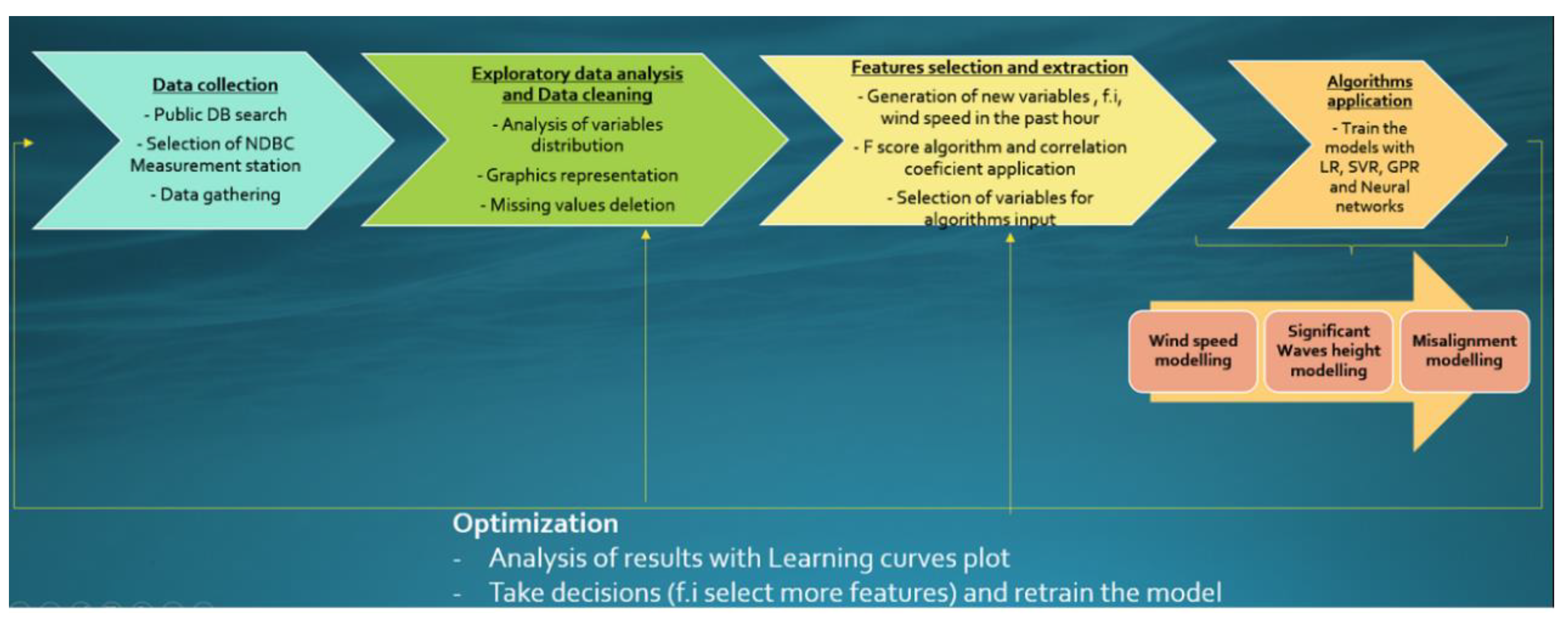
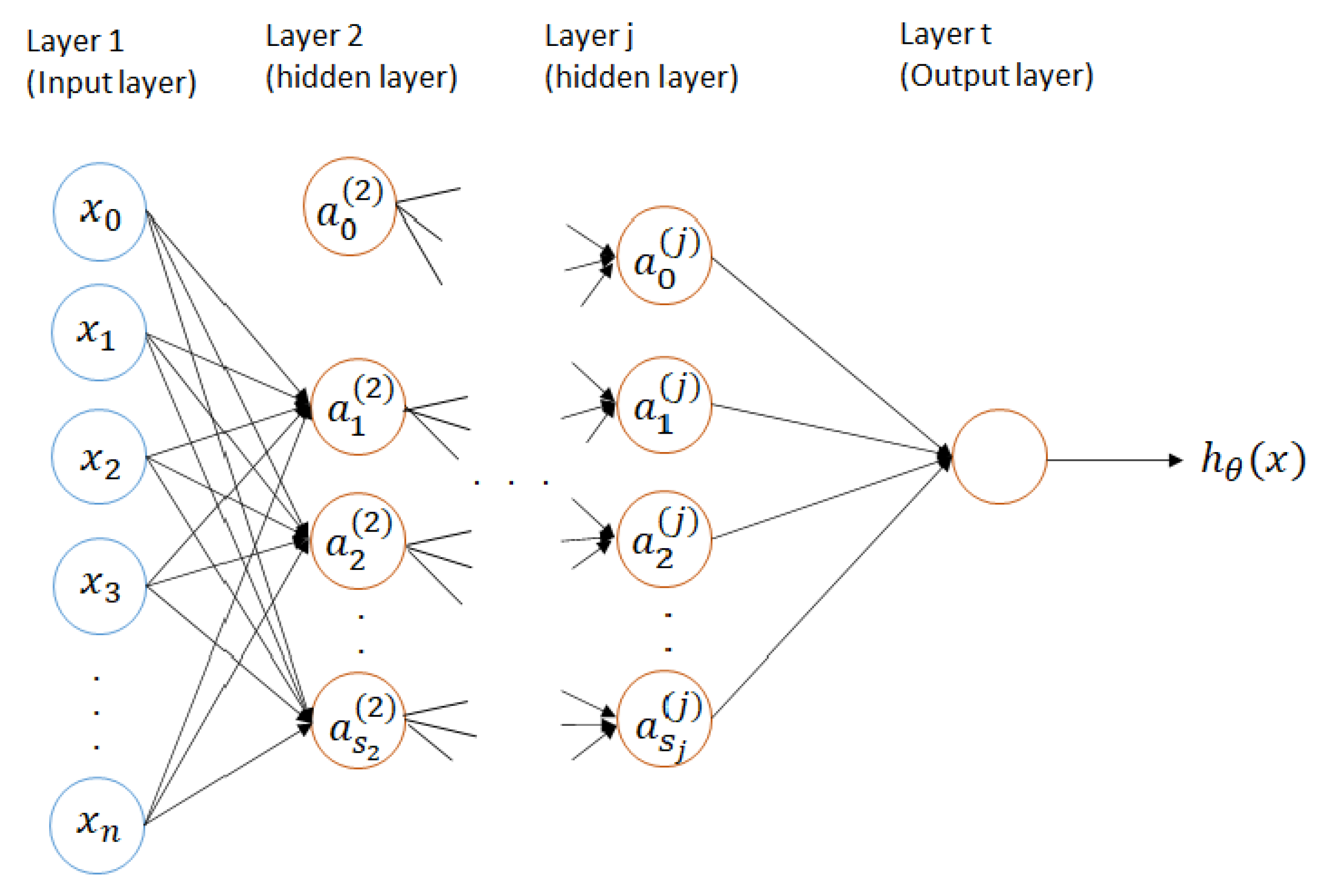
The novelty of this research lies in, on the one hand, the methodology applied that develops all the phases in a machine learning process from scratch (see Figure 1), differing from the most common statistical and physical approaches applied for weather forecasting that are usually found in the literature. However, this general methodology can be applied to any dataset. Another interesting conclusion that can be drawn from the results is that data collection and data pre-processing have proved crucial to obtaining more accurate models. Moreover, data cleaning and analysis help select the most effective machine learning tool to improve the performance of the models and ensure the reliability of such models to make realistic predictions. Finally, to the best of our knowledge, our proposed models for wind–wave misalignment forecasting are robust compared to the existing related literature (see Figure 1 that summarizes the work phases followed in the research).

The structure of the rest of the paper is as follows. Section 2 presents a summary of relevant related works. In Section 3 and Section 4, the materials and methods, respectively, are described. Exploratory data analysis, data cleaning and feature selection are also presented. The optimized models obtained using different ML techniques are discussed and compared in Section 5. Finally, Section 6 concludes the paper with conclusions and future lines of work.

Table 1. Acronyms used.

ANN	Artificial Neural Networks, also denoted as NN (Neural Network)
ARMA	Autoregressive-moving average model
EDA	Exploratory data analysis
FFBP	Feed Forward Back-Propagation
FOWT	Floating Offshore Wind Turbine
GP	Gaussian Process
GPR	Gaussian Process Regression
LDOF	Local Distance-based Outlier Factor
Metocean	Meteorology and Oceanography
ML	Machine Learning
NAR	Nonlinear Autoregressive neural network
NARX	Nonlinear Autoregressive with External (Exogenous) Input neural network
NDBC	National Data Buoy Center
NWP	Numerical Weather Predictions
RBF	Radial Basis Function
SVM	Support Vector Machine
SVR	Support Vector Regression

shows the acronyms used along this paper for better understanding.

2. Related Works

Since the first offshore wind park was installed in Vindeby (Denmark) in 1991, offshore wind farm deployment has grown exponentially, expanding from the North and Baltic Seas to new markets outside Europe [13]. However, although everybody would agree on the importance of analyzing wind and waves to find the best locations for these offshore devices, papers on how wind and waves and particularly how misalignment between those variables, influence energy production are very scarce.

The direct influence of wind speed on the energy power curve of wind turbines and the stochastic and intermittent nature of wind have made its prediction a recurring research topic [14]. According to the type of techniques used, metocean (meteorological and oceanographic) variables forecasting models can be classified into (1) naive, (2) physical, (3) statistical and (4) intelligent models [15,16].

The naive technique (also called the persistence method) is the reference method in industrial applications. It assumes that the wind speed at time t + Δt is the same at time t. Despite its simplicity, it is effective for very short-term and short-term predictions, and it is used in cases when its performance is good enough for that particular application and more complex physical and statistics methods do not achieve a significant improvement [17].

Physical models are based on mathematics and physical considerations like terrain, obstacles, pressure or temperature to estimate wind speed. NWP (numerical weather predictions) and mesoscale models stand out [18]. Generally, the main drawbacks of these models are computational complexity and susceptibility to unstable weather. Despite this, they are suitable for long-term predictions.

Statistical models, such as ARMA or ARIMA, do not need a physical model but statistical distributions and parametric algorithms. They are obtained by curve fitting. These models are adjusted by comparing the actual data and the very last and following predicted values. They are effective for short-term forecasting [19].

Numerous models have been developed using artificial intelligence (AI) and machine learning (ML) techniques [20,21]. Recent examples of wind speed models can be found in the literature, primarily for short-term forecasting. To mention some examples, in [22], a hybrid nonlinear estimation approach combining a Gaussian process (GP) and an unscented Kalman filter (UKF) is proposed to predict dynamic changes in wind speed. In [23], the authors propose an ANN model to predict daily wind speed with meteorological measurements ATMP, WDIR, GHI, relative humidity and PRES as input features selected among the 13 attributes available in the dataset. They applied random forest, random tree, and SVM techniques and compared every model trained with a cross-validation scheme. They used an optimum network with one hidden layer and 30 neurons. Comparing the five different algorithms used, they found that the random forest gave better performance than the other methods.

In [24], traditional MLP neural networks, long short-term memory (LSTM) networks, and stacked auto-encoders are compared in a novel wind-sensitive attention mechanism. A deep neural network results in the best wind forecasting in terms of accuracy. In this paper, the authors used weather forecast information to develop a wind-sensitive attention mechanism for forecasting winds with an LSTM neural network. It has been compared with satisfactory results with the MLP, SVM and EGB (extreme gradient boosting) algorithms. Shahid et al. [25] explored some machine learning techniques for short-term wind speed prediction, specifically random forest (RF), SVR, RBFNN and LSTM, on various wind farm datasets located in Pakistan. For long-term predictions, there are some works, such as the one by Paula et al. [26], where RF, NN and GB were applied to perform regression on wind data for long periods in three wind farms.

Wave height forecasting has always had many applications in coastal and marine engineering design and, more recently, in renewable energies related to ocean resources, such as wave converters and floating wind turbines. Different ML have been applied to obtain models of the significant wave height (WVHT). In [27], the authors present a novel approach to simultaneously tackle short- and long-term energy flux prediction of waves. They considered multi-task evolutionary artificial neural networks (MTEANN) with three different basis functions (sigmoidal unit, radial basis function and product unit) and compared the performance against extreme learning machines and support vector regressors on data of three buoys located in the Gulf of Alaska. In [28], the wave height is modeled with SVR and compared with ANN, MLP and RBF models. Errors obtained for the testing set are: RMSE = 0.21 for SVM with RBF kernel, RMSE = 0.26 for SVM with polynomial kernel, 0.23 for MLP artificial neural network and 0.25 for RBF ANN. In this study, SVM is shown to generalize better than ANN; thus, this technique is considered by the authors to be a more reliable method for offshore energy application. In [29], LSTM wave prediction results were obtained and compared with the MLP, ELM, SVM and RF algorithms. The LSTM network uses past wind speed values, wave height and wind direction. In [30], a near-real-time, half-hourly significant wave height forecast model is designed using a suite of selected model input variables. The multiple linear regression (MLR) model is optimized by a covariance-weighted least squares (CWLS) estimation algorithm to generate a hybridized MLR-CWLS model. The proposed MLR-CWLS model is benchmarked against competing modeling approaches (multivariate adaptive regression splines-MARS, M5 model tree and MLR) using statistical score metrics. Some of them deal with offshore wind turbines but not with floating ones. Other examples related to bottom-fixed offshore turbines are shown in [31], where the authors prove that the exponentiated Weibull distribution provides a better model fit to significant wave height data than the translated Weibull distribution, which is more widely used. Based on 7-year observation data of a buoy station, Zhang et al. [32] present an uncertain accessibility estimation method based on a multi-step probabilistic wave height forecasting model and Monte Carlo simulation to improve offshore wind farm operation and maintenance. However, as shown, there are only a few examples of wave models oriented to floating wind turbines, and they are mainly focused on how the waves affect the response of the turbine instead of on wave height forecasting.

The same happens with papers related to the relationship between wind and waves in floating wind turbines. Although the influence of misalignment on the structural fatigue of FOWT has been studied [21], studies on modeling are scarce. Some notable exceptions are the paper by Hildebrandt et al. [33], which analyzes the occurrence and amount of wind and wave misalignment, as well as the direction dependency of the wind–wave correlation for normal conditions and extreme storms in the German Bight of the North Sea, a location intensively used for offshore wind energy production. Another interesting study is found in [34], where wave height–wind distributions for floating wind turbines are analyzed and modeled. Furthermore, in [35], the conditional joint probability distribution of the significant wave height and peak spectral wave period at the cut-out wind speed is obtained. Then, the stochastic dynamic response and reliability of the FOWT are analyzed considering these loads.

So, as far as we know, it does not seem to be forecasting models of misalignment that can be used for FOWT energy analysis, but some preliminary works, such as the one presented in [36], of which this is an extension.

3. Materials: Data and Pre-Processing

The actual data used in this paper correspond to standard meteorological and descriptive wave measures obtained from the National Oceanic and Atmospheric Administration (NOAA, www.ndbc.noaa.gov) in the USA. Data measurements were taken by sensors equipped with floating offshore buoys distributed through the U.S. and international waters maintained by the National Data Buoy Center (NDBC).

The Santa Maria (CA) station database was selected. This offshore buoy is located in the Pacific Ocean in the northwest of California (34°57′22″ N 121°1′7″ W). Historical files with metocean variables from 2010 to 2020 and real-time files of the last 45 days are available and have been downloaded (indeed from January to April 2020). One of the main reasons for choosing this station was the stability of the weather and sea state, without the strong disturbances that make it suitable for offshore wind turbines. We used the data obtained at 4–5 m height by measuring devices installed on floating buoys. In similar research, it is considered that these data can be extrapolated up to a height of 90 m, that is, about the height of the rotor of the offshore wind turbines. In addition, NDBC buoys are installed about 20–40 km off the coast.

Standard meteorological data files have hourly atmospheric, wind- and wave-related variables averaged values, measured every 8 min. Historical data files are classified by year, while real data files contain the last 45-day measures. The same meteorological features are available in both types of files. The most significant differences between them are the representation of the missing value; in historical files, they are represented by 999 and by ‘MM’ in real-time data files. In addition, reports of measures in real-time files are given each 10 min instead of each hour.

The main features of the data are as follows (

Table 2. Meteorological features measured.

Feature Name	Physical Measure (Units)
YY, MM, DD, HH, mm	Year, month, day, hour, minutes
WDIR	Wind direction (m)
WSPD	Wind speed (m/s)
GST	Gust speed (m/s)
WVHT	Significant wave height (m)
DPD and APD	Dominant and average wave period (s)
MWD	Wave direction (°) in DPD
PRES	Sea level pressure (hPa)
ATMP	Air temperature (°C)
WTMP	Sea surface temperature (°C)
DEWP	Dewpoint temperature (°C)
TIDE	Water level above or below Mean Lower Low Water MLLW (feet)
VIS	Station visibility (nautical miles)

):

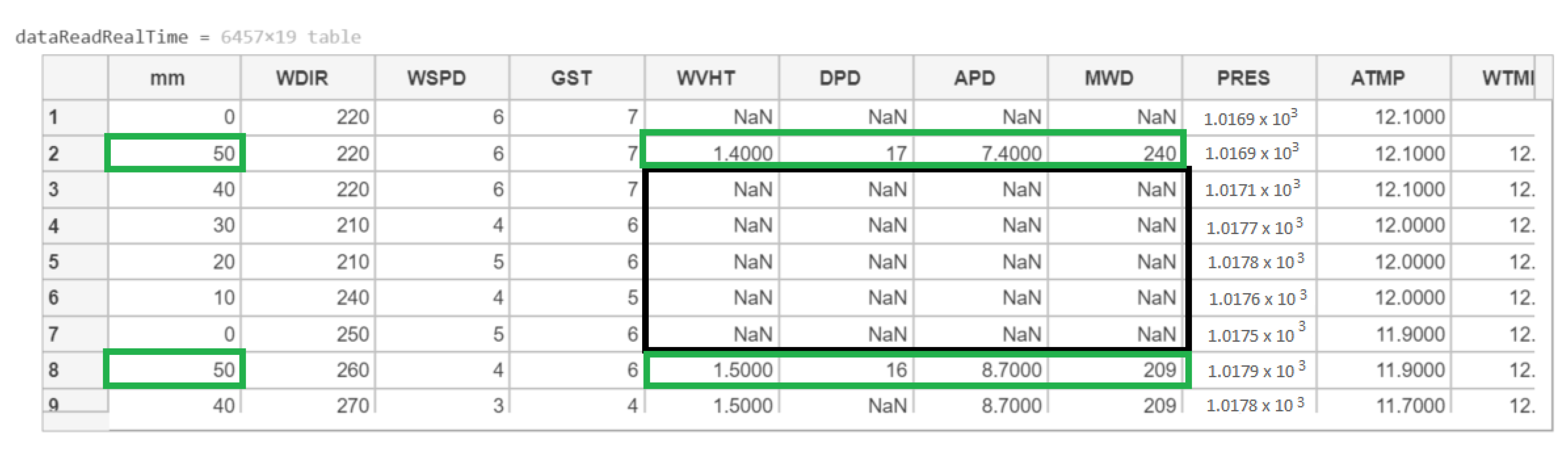
Figure 2 shows a sample of the data downloaded from NDBC website of year 2018 with the corresponding units.

In Figure 3, real-time data from 2020 are presented.

In this Figure 3, some values are within a black square, as an example of values that do not contain any information in contrast to example rows surrounded in green that do not contain missing values. We will deal with this in the following sections.

3.1. Exploratory Data Analysis and Data Cleaning

Exploratory data analysis (EDA) and data cleaning were applied at the same time to the data. As a result of the first visual analysis, it was possible to see (Figure 2) that missing values are represented by a series of 9′s in historical files. Moreover, this data inspection also helped us determine which variables were useless and thus could be removed. For instance, the date variable “minute” was always 50. This is because the measurements are taken every 10 min and reported every hour, so the mm variable can be discarded. Likewise, variables DEWP, TIDE and VIS are always null. These variables are unnecessary for wind and wave forecasting, so we have also ruled them out. In Figure 2, rows in which mm is different from 50 contain NaN values in some important columns, such as WVHT and DPD. This data cleaning was done automatically, with code developed for this purpose.

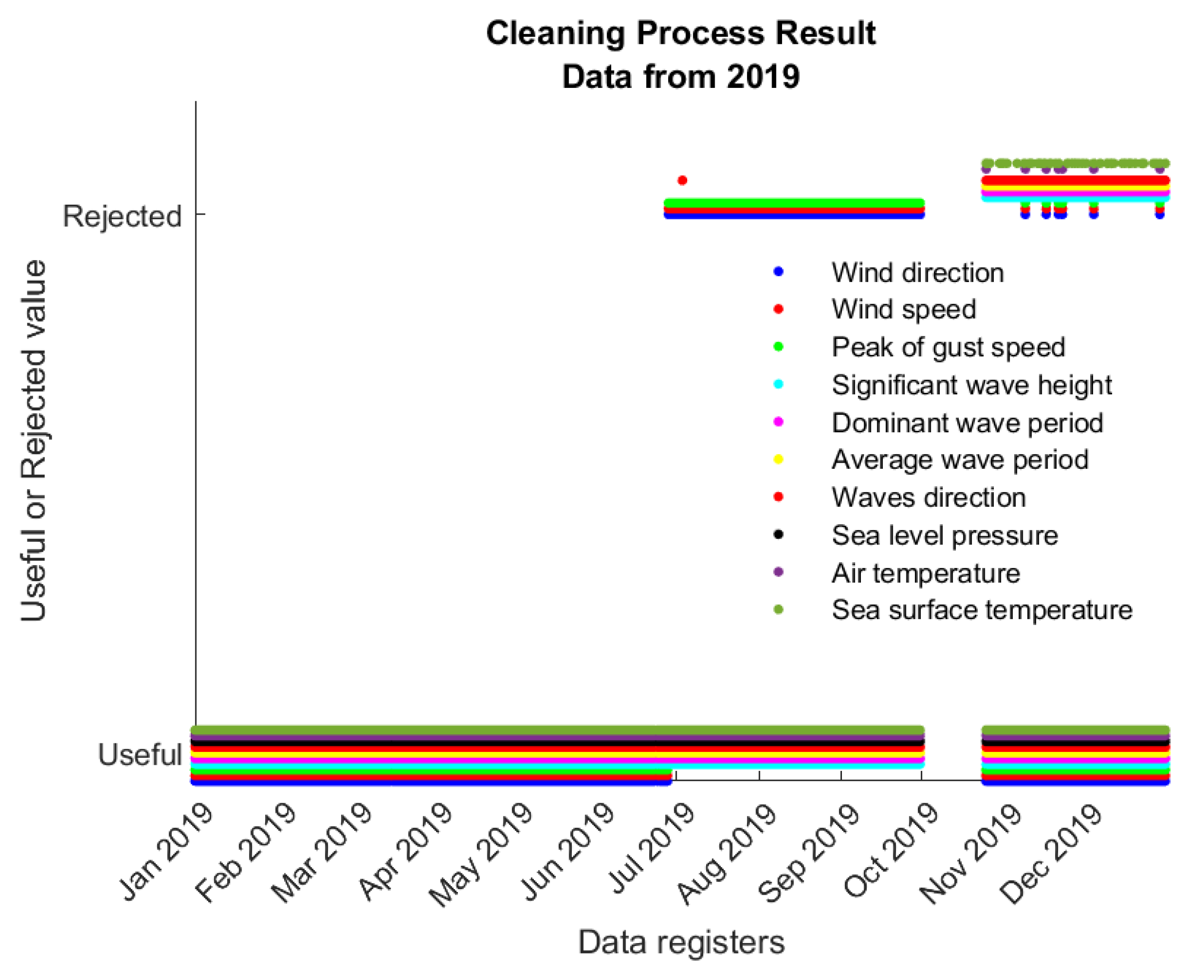
Figure 4 shows an example of the cleaning process results from data from 2019. As a result, rows of data containing missing values were omitted. In addition, it is possible to observe in this figure that the wind direction (blue line) was null in the summer months, so these rows were also removed.

To select the year with more valuable data, the cleaning process was carried out for every available year. The results are presented in

Table 3. Results of the cleaning process for each year.

Year	Initial Rows	Final Rows	% Deleted
2019	16,214	5803	64.20%
2018	8716	8716	0.00%
2017	8685	8684	0.01%
2016	8669	8669	0.00%
2015	8738	5358	38.68%
2014	8750	2444	72.06%

.

Data from 2016 to 2018 were complete, so we worked with them to have enough samples for the model optimization phase. However, if we had needed more data, we could have taken data from 2010.

Outlier detection was carried out to obtain more accurate models. The majority voting method was applied using a graphical boxplot and the LDOF (local distance-based outlier factor) algorithm. The data classified by both methods as outliers were considered anomalous and discarded. We applied this process to a total of 71,031 records, from 2010 to 2020, historical data and to real-time data. The boxplot identified 5333 outliers and the LDOF 4820; from them, 1749 were considered anomalous for both methods and were thus removed.

After data cleaning, we plotted each feature time series, comparing row and clean data to ensure their distributions were the same, and we did not make any mistakes during the cleaning process, so relevant information was not missing. The deletion of the outliers had the effect of expanding the graph as the upper limit was reduced.

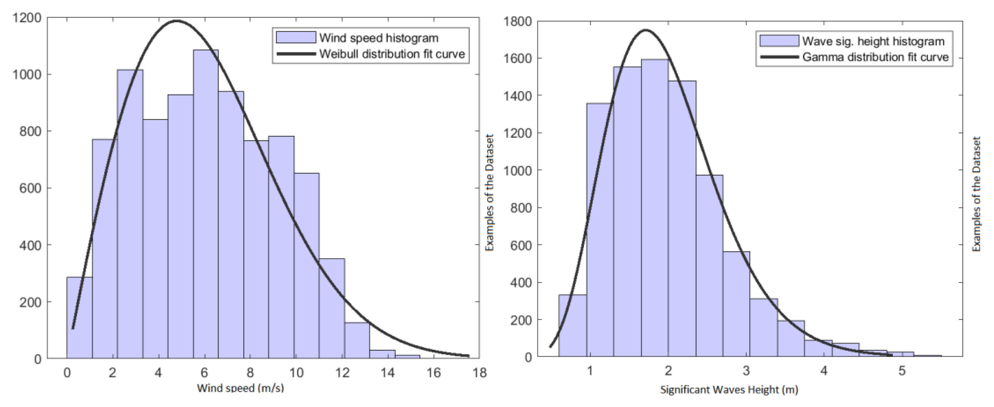
Subsequently, univariate analysis was carried out for each variable. The central (mean, median, mode), spread (range, standard deviation, variance and quartiles), and shape (central moment, maximum and minimum) values were calculated. The distribution that best fit the data was found. Figure 5 (left) shows how the wind speed variable in the Santa Maria station is concentrated around its mean and is relatively stable, and Figure 5 (right) is the same for significant wave height. The Weibull distribution fit the data accurately, as shown in these figures. The statistical values of these measures are shown in

Table 4. Statistical measures of wind and wave variables.

		Wind Speed	Wave
Central measures	mean	6.0450	1.9779
	median	6	1.87
	mode	6.4	1.67
Spread measures	range	15.4	4.82
	std	3.1328	0.7523
	variance	9.8145	0.5660
	quartiles	[0, 3.4, 6, 8.5, 15.4]	[0.67, 1.42, 1.87, 2.39, 5.49]
Shape measures	central mom	5.1228	0.4237
	max	15.4	5.40
	min	0	0.67

.

Statistical analysis was carried out for all the different metocean variables, but some of them, such as wind and wave directions, were circular and analyzed with different tools. For instance, we used the wind rose to visualize the relationship between wind speed and wind direction.

3.2. Feature Selection

Feature selection, also known as variable subset extraction, consists of selecting a subset of relevant predictors from all existing features for modeling. To carry out feature selection, we first applied the F-test, which calculates univariate feature ranking (based on the covariance measure). Then, all predictors were ordered by importance in the dataset and had an associated weight.

Correlation analyses, Pearson and Spearman correlation coefficients for pair-wise features, were also performed, obtaining similar values with both approaches. Annual linear correlation matrixes for 2016, 2017 and 2018 were calculated to demonstrate that the annual correlation remains between variables regardless of the particular year. We highlighted some pairs of highly correlated variables, such as WVHT-WDIR or WSPD-GST, that were, therefore, discarded to avoid including redundant information.

For each of the forecasting models that would be obtained, the following potential predictors were selected:

• Wind speed forecasting: WSPD (target), WDIR, ATMP, PRES;
• Significant wave height prediction: WVHT (target), WSPD, WDIR, MWD, WTMP, PRES;
• Misalignment forecasting: MIS (target), WVHT, WSPD, PRES, WTMP.

During the modeling, we tried different combinations of features from each subset.

For misalignment forecasting, we combined wind direction (WDIR) and wave direction (MWD) to obtain a new feature representing the wave and wind misalignment, called MIS. To obtain the misalignment, we first subtracted the angle of the wind and wave direction. We then calculated the rest by dividing the resultant angle by 180°.

Finally, we incorporated a temporal window of the previous values for time series forecasting.

4. Methods: Machine Learning (ML) Techniques

Through machine learning algorithms, we can gain insight into the collected data [37]. Matlab software was selected for data pre-processing and ML techniques implementation in this research. The ML algorithms applied for predictive modeling are summarized below.

4.1. Linear Regression (LR)

The hypothesis function established a linear relationship between input variables and output, as follows:

$$h_{\vartheta }\left(x\right)={\theta }_0+{\theta }_1{x}_1+{\theta }_2{x}_2+\dots +{\theta }_n{x}_n$$

(1)

where ${\theta }_0$, ${\theta }_1$,…, ${\theta }_n$ are model parameters and $x_1$,…, $x_n$ are the components of an input example. ${\theta }_0$ represents the bias or offset.

The cost function used to measure the accuracy of the hypothesis function was $\frac{1}{2}$ multiplied by the “squared error function” or “mean squared error” (MSE), which is the mean of the differences between the predicted value and the actual output value for every example in the dataset.

$$J\left({\theta }_{0,}{\theta }_1,\dots ,{\theta }_n\right)=\frac{1}{2m} {\displaystyle \sum }_{i=1}^m{\left({\widehat{y}}_i-y_i\right)}^2=\frac{1}{2m}{\displaystyle \sum }_{i=1}^m{\left(h_{\vartheta }\left(x_i\right)-y_i\right)}^2$$

(2)

The algorithm updates the $\theta$ parameters vector for every input training example $\left(x^{\left(i\right)}, y^i\right)$ by minimizing the cost function.

4.2. Gaussian Process Regression (GPR)

Gaussian process regression (GPR) is a non-parametric Bayesian approach to regression [38]. It infers the probability distribution over all admissible functions that fit the data (function-space view).

Gaussian process comes specified by a mean function $m\left(x\right)$ and the Kernel covariance function $k\left(x, x^{\prime }\right)$ of a real process $f\left(x\right)\mathcal{G}P\left(m\left(x\right),k\left(x, x^{\prime }\right)\right)$, so:

$$y \mathcal{G}P\left(m\left(x\right),k\left(x, x^{\prime }\right)+{\delta }_{ij}{\sigma }_n^2\right)$$

(3)

We specified the mean function and covariance kernel function, which were tuned during the optimization phase. The following kernel functions were selected: constant, linear square exponential, Matern kernel or a combination of some of them. For instance, the combination of the constant kernel with the radial basis function (RBF) kernel is widely used:

$$k\left(x,x^{\prime }\right)={\sigma }_f^2\exp \left(-\frac{1}{2l^2}x-{x^{\prime }}^2\right)$$

(4)

where ${\sigma }_f^2$ and $l$ are the hyper-parameters that must be tuned.

4.3. Support Vector Machines for Regression (SVR)

Support vector machine (SVM) or “large margin classifier” tries to find the line or hyperplane that best separates observations of the training set into different output classes. The regression problem is a classification problem with infinite output classes (continuous output variables). Thus, SVR introduces a $ϵ$-sensitive region around the function $y$ that we want to predict, called the $ϵ$-tube. The SVR optimization problem consists of finding the tube:

$$f\left(x\right)={\theta }^{T}x+b$$

(5)

This best approximates the continuous-valued function [39]:

$$\parallel y_i-{\theta }_i{x}_i\parallel \le ϵ$$

(6)

4.4. Neural Networks (NAR, NARX and Feed-Forward NN)

An artificial neural network (NN) is a computational solution for machine learning applications. An artificial neuron receives input examples with n features from its neuron synapsis. Then, it returns an output $h_{\theta }\left(x\right)=f\left(x\right)$ that is calculated considering the “weights” assigned to each input connection and an activation function $f$ assigned to the neuron, also known as a transfer function, where $x_0$ corresponds to the bias unit (see Figure 5).

That is, the neuronal model is: $h_{\theta }\left(x\right)=f\left({\theta }_0+{\theta }_1·x_1+{\theta }_2·x_2+\dots +{\theta }_n·x_n\right)$. We have tried different transfer functions $f$ such as the linear transfer function (also called Purelin): $f\left(h_{\theta }\left(x\right)\right)=h_{\theta }\left(x\right)$, Log-sigmoid function $f(h_{\theta }\left(x\right)=\frac{1}{1+\exp -h_{\theta }\left(x\right)}$ or Hyperbolic tangent sigmoid function (also called Tansig): $f(h_{\theta }\left(x\right)=\frac{2}{1+\exp -2·h_{\theta }\left(x\right)}-1$.

Figure 6 shows the neural network model representation, where:

$$a_i^{\left(j\right)}=f\left({\theta }_{i,0}^{\left(j-1\right)}{x}_0+{\theta }_{i,1}^{\left(j-1\right)}{x}_1+\dots +{\theta }_{i,s_{j+1}}^{\left(j-1\right)}{x}_{s_{j+1}}\right)=f(z_i^{\left(j\right)})$$

(7)

Hence, the hypothesis function is represented by:

$$h_{\theta }\left(x\right)=a^{j+1}=f\left(z^{j+1}\right)$$

(8)

where, in this case, $j=$ last hidden layer and $j+1=$ output layer.

A well-known backpropagation algorithm was applied to train the neural network.

A nonlinear autoregressive neural network (NAR), which relates the current value of the time series to the past values of the time series, was also applied. Moreover, the nonlinear autoregressive with exogenous neural networks (NARX) that relate the current value of the time series with current or past external series (other features of time series that influence the time series we want to forecast) [40] was also considered.

The NAR model that predicts $y\left(t\right)$ series can be represented by the following expression:

$$y\left(t\right)=f\left(y\left(t-1\right),y\left(t-2\right),\dots ,Y\left(t-d\right)\right)$$

(9)

NARX model can be represented with the function:

$$y\left(t\right)=f\left(x\left(t-1\right),\dots ,x\left(t-d\right), y\left(t-1\right),\dots ,y\left(t-d\right)\right)$$

(10)

5. ML-Based Models and Discussion of the Results

The five ML techniques described above were applied to real data of the metocean variables of the buoy. After the training phase, if the model obtained gave an unacceptable classification ratio, we still evaluated the models using the learning curves plot tool. In this way, it was possible to determine whether the problem was due to high bias or high variance. This information may help us optimize the model better, choosing more examples to be included in the training dataset or fewer features, for instance.

In the regression learner tool, the hold-out validation scheme was configured with a held-out data subset of 20% for the regression algorithm application. This means that 20% of the 8581 rows were used for validating the models with unseen observations.

In the case of artificial neural networks, the dataset was split into training (70%), validation (15%) and testing (15%) sets. Finally, the best models were tested with data from 2019 and 2020 (“Real-Time”) to evaluate their performance.

The performance was measured with the root mean square error (RMSE), in m/s for wind speed, in m for wave height, and in degrees for misalignment. The RMSE was calculated as follows:

$$\mathrm{RMSE}=\sqrt{\frac{1}{m}{\displaystyle \sum }_{i=1}^m{\left(h{\left(\theta \right)}^i-y^i\right)}^2}$$

(11)

The success rate, $S_r$ (%), which is the percentage of correct predictions made by the model, is:

$$S_r=\left(1-\frac{\mathrm{RMSE}}{max}\right) \%$$

(12)

The best models obtained for each variable were selected. They are presented here regarding the variables that predict wind speed, significant wave height, and wind–wave misalignment.

5.1. Wind Speed Models

Models were trained to forecast the next hour’s wind speed by trying different combinations of features of the dataset for the year 2018. If necessary, more data from other years were added to the training set during the optimization phase.

Linear regression was the first algorithm we applied because of its simplicity and ease of understanding. Model variants, namely linear, interactions linear, robust linear and stepwise linear, were also tested in next hour wind speed forecasting. All regressions gave the same results (RSME = 1.0546, MAE = 0.7837) except for the robust variant, which gave RMSE = 1.0558 and MAE = 0.7819, and the best success rate, 93.14%, although the rest gave 93.15%.

We also obtained the results of linear regression models trained with 1-h to 6-h previous wind speed data. The wind models obtained with the two and three last hours’ wind speeds as input show the smallest cross-validation errors.

With these results in mind, we applied support vector machines for regression, initially trained with data from 2018 and two last hour wind speed values as predictors. Different configurations were tested, obtaining the best results with Gaussian kernel function, a box constraint of 9.78 and ε = 0.066. The results were RMSE = 1.0359 and MAE = 0.7664, with a success rate of 93.27%.

To improve the SVR model, we first plotted its learning curves when training the model with different subsets of m training examples and then calculated the training and validation RMSE for each m. Next, a threshold to stop optimization of the algorithm was defined, called a reference error. According to the range of errors found in the literature for models that predict this variable with the learning curves, the reference error was set to 0.9.

The best configuration found was the SVR model with 1 to 10 h previous wind speed data, linear kernel function, a box constraint of 6.1141 and ε = 0.1377; and with 1 to 14 previous hourly wind speed data, Gaussian kernel function, box constraint of 0.5056 and ε = 0.0096 (success rate 93.41% and 93.52%, respectively).

Gaussian process regression model was trained with the wind speed from the previous hour as a predictor. The best configuration was the isotropic Matern 5/2 kernel function, with a kernel scale of 0.0164 and $\sigma =0.0057$ as hyper-parameters, which gave an RMSE = 1.0424 and MAE = 0.7746 (success rate: 93.23%). Even though this model gave a good performance compared with our reference error, to further improve it, we trained the GPR models with wind speed, air temperature and pressure of the one and two last hours as predictors, obtaining an RMSE = 1.0258 and MAE = 0.7630 (success rate of 93.34%) for the las hour variables as predictors, which make it the best GPR model obtained.

To determine whether we could obtain better models, we applied nonlinear autoregression neural networks with the wind speed variable as a predictor. The initial network was configured with 15 neurons in the hidden layer and a delay of 6, giving an RMSE for the training set of 1.0235, 1.0581 for the validation set, and an error for the testing set of 1.0871 (success rate = 92.94%). Plotting these results in learning curve plots gave us the intuition that this model suffered from high variance. A NAR model with 15 neurons and 1 as the delay gave the best RMSE for the testing set: 0.9762 (success rate of 93.66%). Nonlinear autoregressive with external input (NARX) neural networks were trained with air temperature, pressure and wind direction as predictors, and wind speed as the target variable. Different combinations were tried, obtaining the best NARX with 9 neurons in the hidden layer and a delay of 6, trained with data only from 2018, giving an RMSE for the testing set of 0.9893 (success rate of 93.58%).

Wind Speed Model Comparison

Table 5. Best model results for WSPD forecasting for each ML algorithm.

Algorithm	Model	RMSE (Validation)	RMSE (Test Data 2019)	RMSE (Test Data 2020)	Success Rate (Validation)
LR	wind_lr2	1.0529	1.1237	1.1723	93.16%
SVR	wind_svm3	0.9985	1.1462	1.1722	93.52%
GPR	wind_gpr2	1.0285	1.1344	1.1670	93.32%
NAR	wind_nar3	0.9762	1.1496	1.1713	93.66%
NARX	wind_narx2	0.9988	1.1124	1.1340	93.51%

shows the performance of the best models obtained with each ML technique for wind speed forecasting.

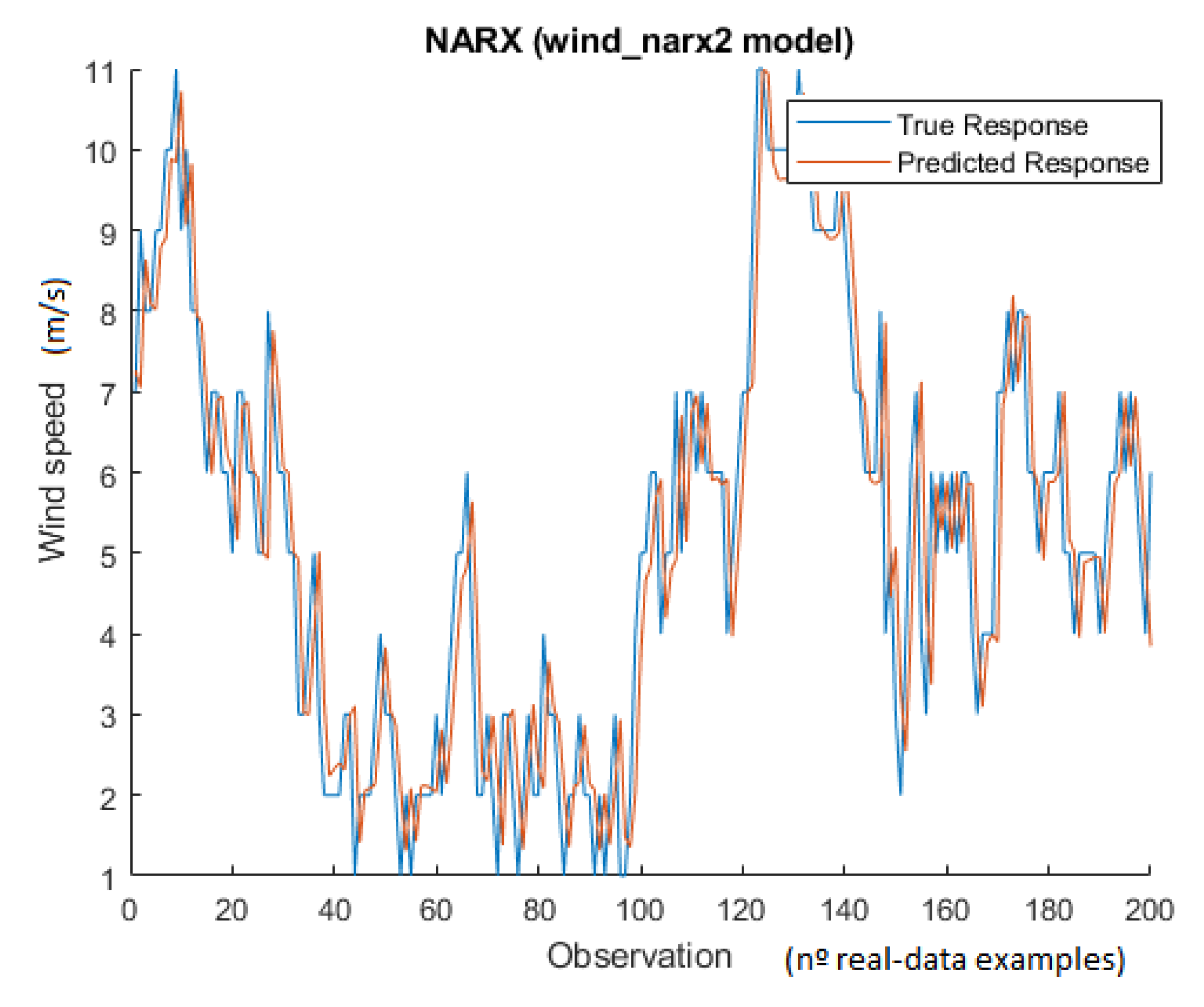
Although the wind_nar3 model had the best validation success rate (93.66%), it generalizes worst for 2019 and 2020 data forecasting, as observed in the RMSE values for those years. The algorithm that performed the best regarding the validation RMSE (0.9988, the second smallest) and the smallest RMSE for 2019 (1.1124) and 2020 (1.1340) was the nonlinear autoregressive with external input neural network (NARX) algorithm, with a success rate of 93.51%. The best configuration found for this ML algorithm was:

• Dataset: data from 2018;
• Predictors: WSPD, ATMP, PRES, WDIR;
• N° neurons in the hidden layer: 5;
• N° input delays: 3 h before forecasting moment (t).

Figure 7 shows the predicted wind speed against the actual output values for 2020.

5.2. Significant Wave Height Prediction

Models to predict significant wave height in the frequency domain have been trained based on wind and other weather known variables and wave direction. Initially, we considered the data from 2018 for the dataset.

We started applying the linear regression (LR) algorithm based on the high linear correlation between wind speed and wave height. First, the LR model was trained with wind speed as a predictor; the 5-fold cross-validation schema partition was used for the dataset, giving RMSE = 0.6747 and MAE = 0.5149 (success rate of 87.71%). In the optimization phase, we included wind and wave direction as predictors in addition to wind speed, obtaining a bit smaller RMSE = 0.6290 and MAE = 0.4749 errors and a slightly better success rate of 88.54%.

As for the wind, we also applied the support vector machine for regression (SVR) to see if we could obtain better results. The configuration of SVR with Gaussian kernel function, wind speed (WSPD), wave direction (MWD), and wind direction (WDIR) as predictors, and 20% hold-out cross-validation schema applied to the dataset, gave RMSE = 0.5889 and MAE = 0.4312 (success rate = 89.27 %). The learning curves showed noisy values, which means that the training dataset could be unrepresentative of this problem. Therefore, we selected an additional predictor: sea surface temperature (WTMP) and applied the 5-fold CV instead of the 20% hold-out CV scheme, obtaining a LR model with RMSE = 0.5203 and MAE = 0.3709 (success rate of 90.52%).

With the Gaussian process regression (GPR) algorithm and WSPD, MWD and WDIR as predictors, we obtained a model with RMSE = 0.5820 and MAE = 0.4373 (success rate of 89.39%). Then, we tried to improve this model, which suffered a high bias as per the learning curves plot, adding pressure (PRES) and WTMP measures as additional predictors and adding the data from 2017 to the dataset, obtaining a GPR model that gave RMSE = 0.5021 and MAE = 0.3755 (success rate of 90.85%).

Feed-forward backpropagation artificial neural networks (ANN) were used for the significant wave height prediction. A network with 1 hidden layer of 15 neurons, WDIR, WSPD and MWD as predictors, and training function Trainlm gave an RMSE(Train.) = 0.5130, RMSE(Valid.) = 0.5533 and RMSE(Test) = 0.5365 (success rate of 90.22%). Since this network had high bias, we tried different configurations to obtain the best ANN with 4 hidden layers (20, 25, 7 and 2 neurons, respectively), WSPD, WDIR, MWD, PRES and WTMP as predictors, and training function trainlm, which eventually gave RMSE(Train.) = 0.4214, RMSE(Valid.) = 0.4947 and RMSE(Test.) = 0.4517 (success rate of 91.77%)

Significant Wave Height Model Comparison

We compared the best models obtained with each ML technique for the significant wave height prediction; the results are presented in

Table 6. Best model results for WVHT prediction for each ML algorithm.

Algorithm	Model	RMSE (Validation)	RMSE (Test Data 2019)	RMSE (Test Data 2020)	Success Rate (Validation)
LR	waves_lr2	0.6290	0.7877	0.5692	88.54%
SVR	waves_svm2	0.5679	0.8174	0.6149	89.66%
GPR	waves_gpr3	0.5021	0.7312	0.6940	90.85%
Feed-forward ANN	waves_ann3	0.4517	0.8112	0.7421	91.72%

.

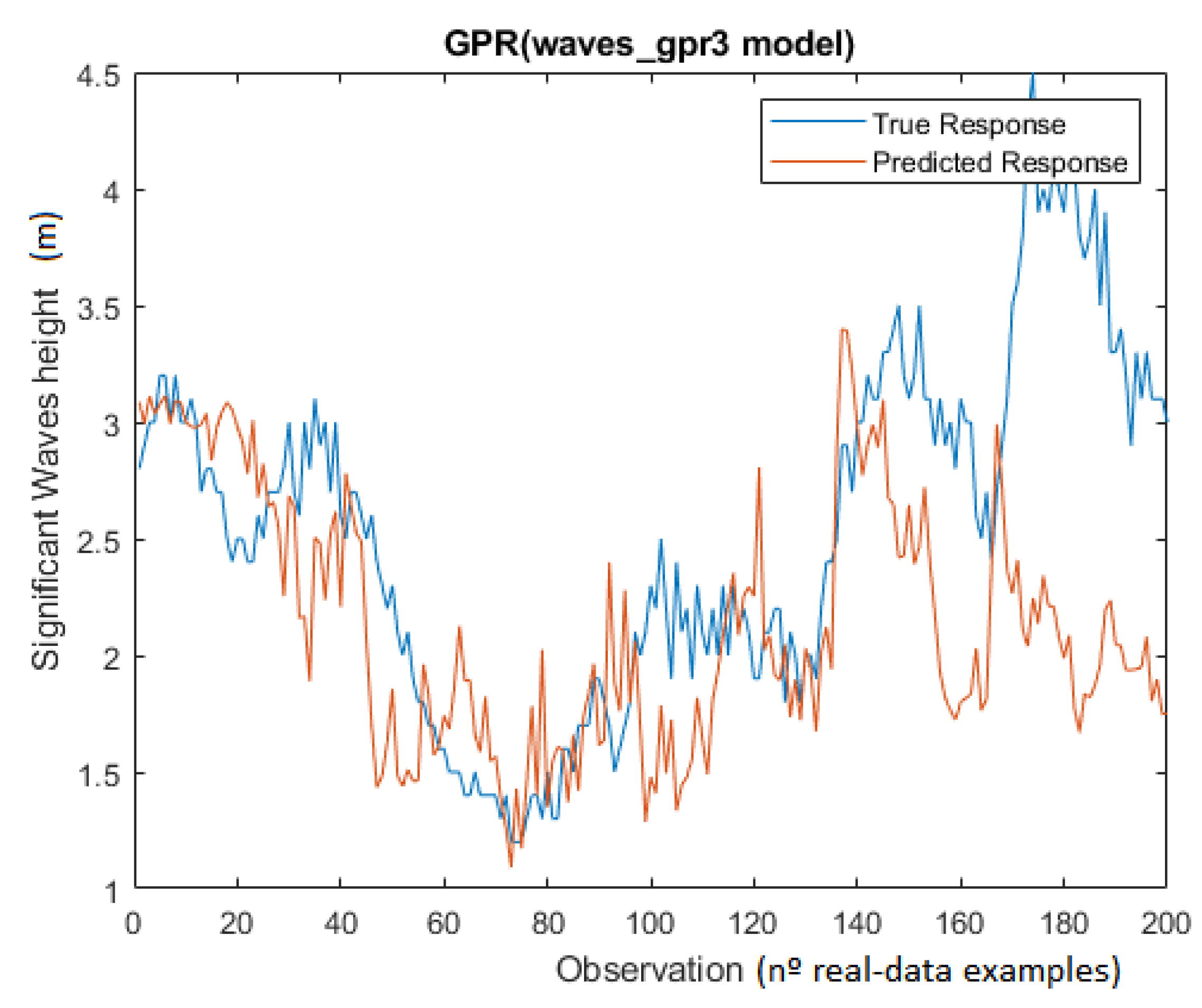
Although the feed-forward ANN had the highest validation success rate (91.72%), the best algorithm to predict WVHT is the Gaussian Process regression (GPR) with the second-lowest validation RMSE (0.5021) and the best RMSE for test data for 2019 (0.7312) and for 2020 (0.6940). The waves_gpr3 model configuration that gave the best results was:

• Dataset: data from 2018;
• Predictors: WSPD, WDIR, MWD, PRES, WTMP.

Figure 8 shows the predicted significant wave height against the real output values for 2020.

5.3. Misalignmet Model

Wind and wave misalignment forecasting is a novel but necessary task; indeed, models for misalignment (MIS) forecasting have not been found in the literature. Due to this, the reference error selected has been defined using some knowledge, considering 90° an acceptable limit MIS for FOWT.

The models were trained to forecast the next hour’s misalignment. The selected dataset contained data from 2018, and when necessary, more data was added during the optimization phase to improve the convergence. The RMSE of the angle was measured in degrees.

First, we trained the linear regression (LR) model with MIS values from the last hour as predictors, giving an RMSE = 53.9260 and MAE = 32.67.21 (success rate of 70.04%). Adding as predictors the values of the following variables: sea surface temperature (WTMP), wind speed (WSPD) and sea level pressure (PRES) from the last hour, the LR model improved slightly, giving an RMSE = 52.1342 and MAE = 30.8361 (success rate of 71.04%)

The first trained support vector regression (SVR) model yielded similar performance results. SVR was applied with the Gaussian kernel function and current MIS as the predictor, giving RMSE = 54.8385 and MAE = 29.9080 (success rate of 69.53%). To ensure the performance of this model, we tested it with data from 2019 and 2020, obtaining RMSE = 63.5201 and 65.4028, respectively. To improve the success rate, we trained the model with two more predictors: wind speed (WSPD) and sea surface temperature (WTMP), resulting in a model that had an RMSE = 51.9623 and MAE = 31.9612 (success rate of 71.13%).

Gaussian Process Regression (GPR) was also applied with the goal of obtaining a better success rate. GPR model with MIS, WSPD and WTMP from the last hour as predictors gave an RMSE = 51.5981 and MAE = 31.2231 (success rate of 71.33%). An angle of 50° is 40° smaller than the initial reference error of 90° so the Learning curves showed that this model fit the data well, and the validation curve was below the training curve, one of the objectives.

Nonlinear autoregressive neural networks (NARs) were proven to forecast MIS satisfactorily. The first NAR model consisted of one hidden layer with 10 neurons and was trained with the Lavenberg-Marqueardt algorithm and with last hour MIS values as input (delay of 1), giving an RMSE(Train.) = 53.1438, RMSE(Valid.) = 54.0507 and RMSE(Test) = 53.6406 (success rate of 70.20%). The same NAR configuration was trained with the Bayesian Regularization Backpropagation function, giving a better RMSE(Train) = 50.3944 and RMSE(Test) = 49.7858 (success rate of 72%).

Finally, nonlinear autoregressive with exogenous input networks (NARX) were trained. Initially, the NARX model was configured with one hidden layer of 10 neurons and trained with last two hours values (delay = 2) using MIS and WSPD as predictors, which gave an RMSE(Train.) = 51.6333, RMSE(Valid.) = 52.7523 and RMSE(Test) = 49.0421 (success rate of 72.75%). To decrease the RMSE(Valid.), a NARX model with 8 neurons in the hidden layer and the last two hours MIS and WSP values was tested, using more data (from 2010 to 2018) for the training, giving an RMSE(Train.) = 51.1227, RMSE(Valid.) = 50.5203 and RMSE(Test) = 50.3699 (success rate of 72.02%).

Misalignment Model Comparison

Table 7. Best model results for MIS forecasting for each ML algorithm.

	Model	RMSE (Validation)	RMSE (Test Data from 2019)	RMSE (Test Data from 2020)	Success Rate (Validation)
LR	mis_lr2	52.1342	62.4652	66.2944	71.04%
SVR	mis_svm2	51.9623	61.7990	64.3001	71.13%
GPR	mis_gpr2	51.5981	59.7840	62.7212	71.33%
NAR	mis_nar2	49.7858	61.8016	62.7157	72.34%
NARX	mis_narx2	50.3699	58.1550	61.5061	72.02%

shows the performance of the best models obtained with each ML technique for MIS forecasting.

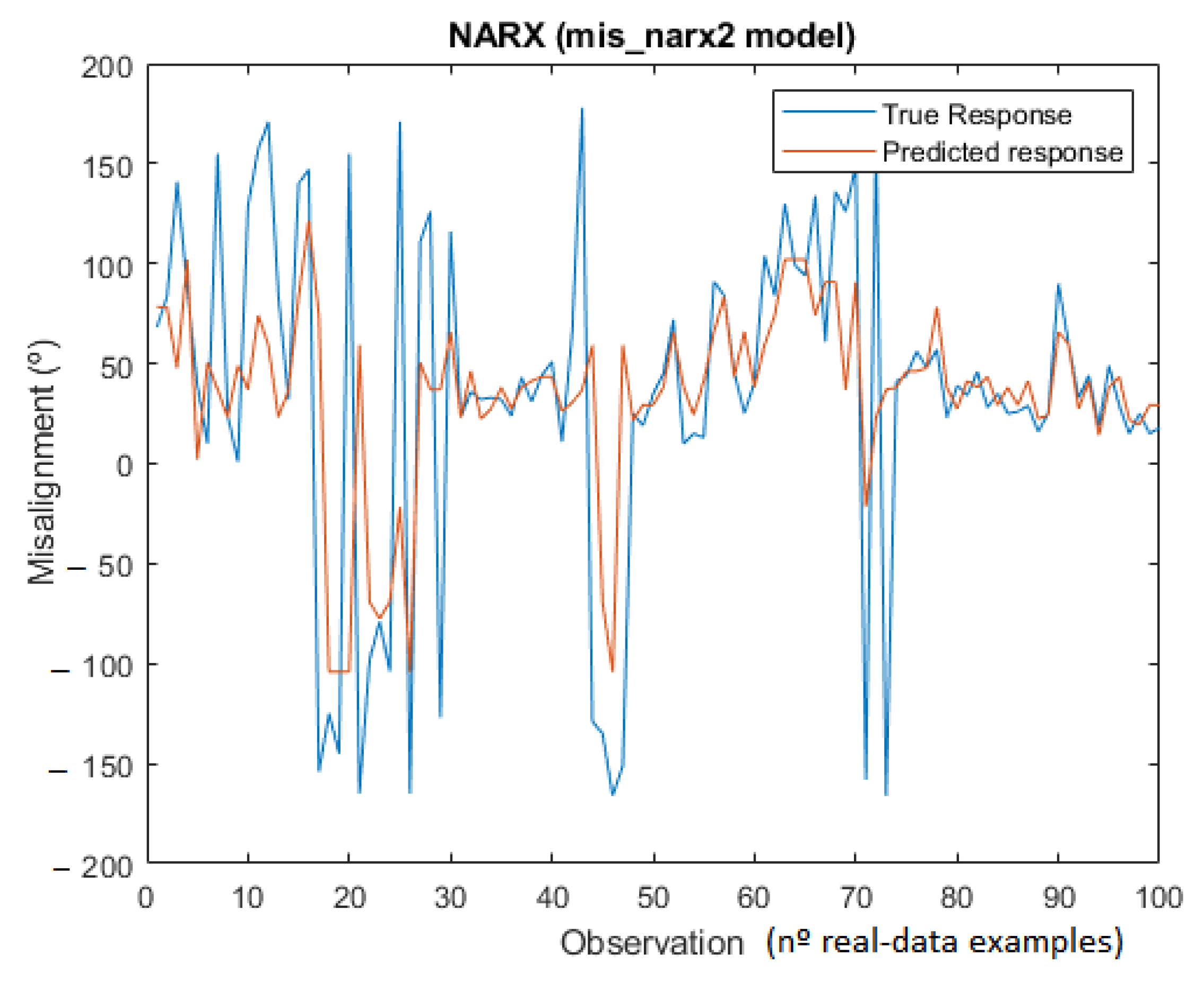
Table 7 shows that Nonlinear Autoregressive with External Input (NARX) Neural Network (bolded) outperformed the other algorithms for misalignment forecasting. Although the mis_nar2 model has smaller RMSE validation than the mis_narx2 network, the latter outperformed the first one for new data from 2019 and 2020. The optimal configuration for the mis_narx2 model was:

• Dataset: data from 2010 to 2018;
• Predictors: MIS and WSPD;
• N° neurons in the hidden layer: 8;
• N° input delays: 2 h before the forecasting moment (t).

Figure 9 shows the predicted misalignment against the real output values for 2020.

6. Conclusions and Future Works

In this work, different ML techniques were tested to obtain predictions of metocean variables. The ultimate goal is to obtain good models that find the best location for offshore wind turbine deployment. To do so, three variables that have a significant impact on the electrical energy produced by a floating wind turbine have been studied: the wind speed, the significant height of the waves and the misalignment, which is calculated as the difference in the direction of the wind and the waves.

Various ML techniques have been tested with different configurations to study whether they can obtain good prediction models. In general, some specific configuration of each ML method applied has been found that gives satisfactory results for forecasting ocean variables. However, the neural NARX network seems to outperform the other tested algorithms (SVR, LR, GPR, NAR and MLP), mainly for wind speed forecasting. The GPR model proved to be the most accurate for significant wave height prediction in the frequency domain. In the literature, we have not found models for wind–wave misalignment forecasting, a relevant variable for floating wind turbine locations. Among all the models trained, the NARX algorithm has become the most efficient in this respect.

Correct evaluation of the proposed models with techniques, such as learning curve plots, was also essential to optimize the models and make better decisions regarding the best configuration.

In future work, it would be interesting to apply the proposed methodology to other metocean data from different offshore locations. This would allow us to study how much a particular site for a wind farm location influences model performance. Furthermore, it would be of interest to test the already-trained models with real data from different locations and observe whether the success rates are maintained. In addition, the creation of hybrid models that integrate these models into more sophisticated predictive systems for wind power or wind turbine fatigue prediction is proposed, which will help maintenance [41]. Finally, extending the prediction horizon could be another future line of research.