
Formation Control of Multiple Autonomous Underwater Vehicles under Communication Delay, Packet Discreteness and Dropout

 ,
,
Abstract
:1. Introduction
- (1)
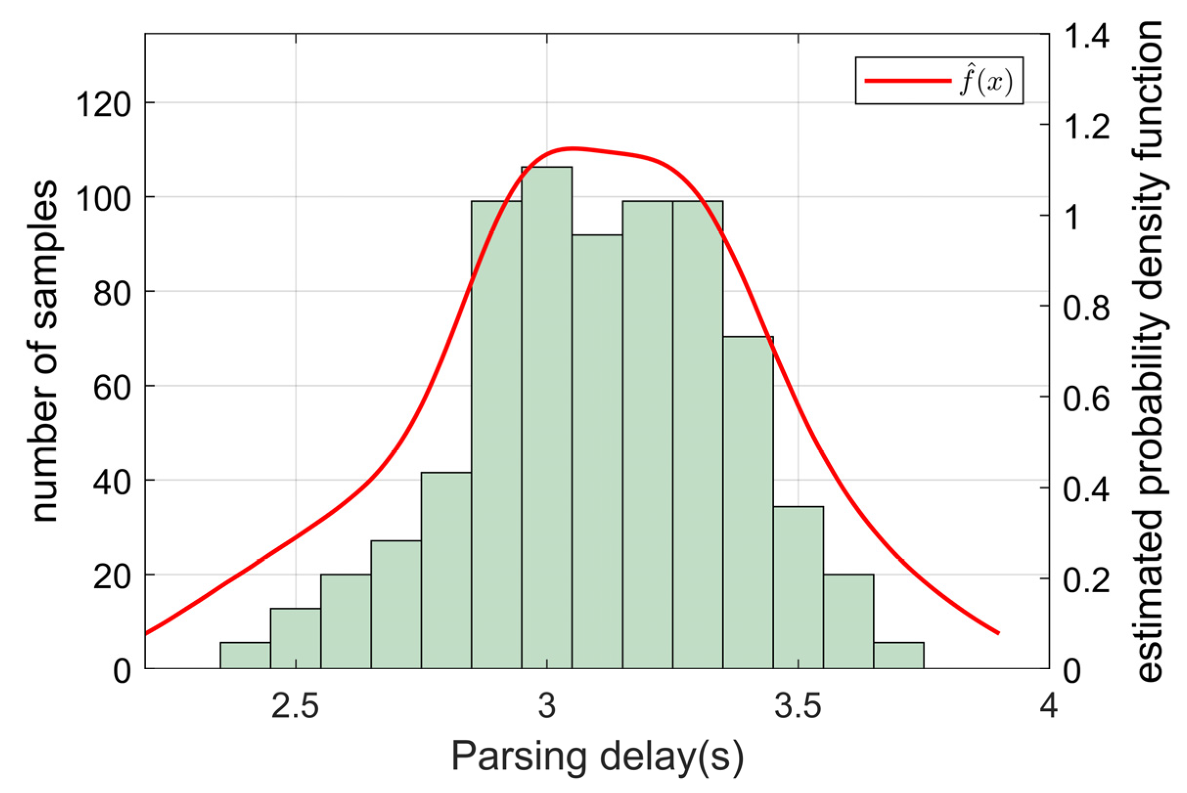
- The communication delay is estimated based on the kernel density estimation method. Kernel density estimation is a non-parametric estimation method that does not need prior knowledge and an accurate mathematical model of communication delay. Instead, we can obtain an accurate distribution of delay with this method according to the characteristics and properties of delay values based on underwater experiments. Compared with other methods, this method has more extensive applications.
- (2)
- The packet discreteness and dropout problems are solved by information prediction based on the curve fitting method. This method can be used to predict the key states of the leader AUV to generate a continuous and precise trajectory for the follower AUVs.
- (3)
- We derive a kinematic model for the error of the formation control system. The follower controller is designed using the input–output feedback linearization method and the stability of this method is proved by Lyapunov stability theory.
- (4)
- Both the simulation in MATLAB and the field tests on the lake are carried out to verify the feasibility of the scheme presented in this paper.
2. Problem Formulation and Preliminaries
2.1. AUV Model
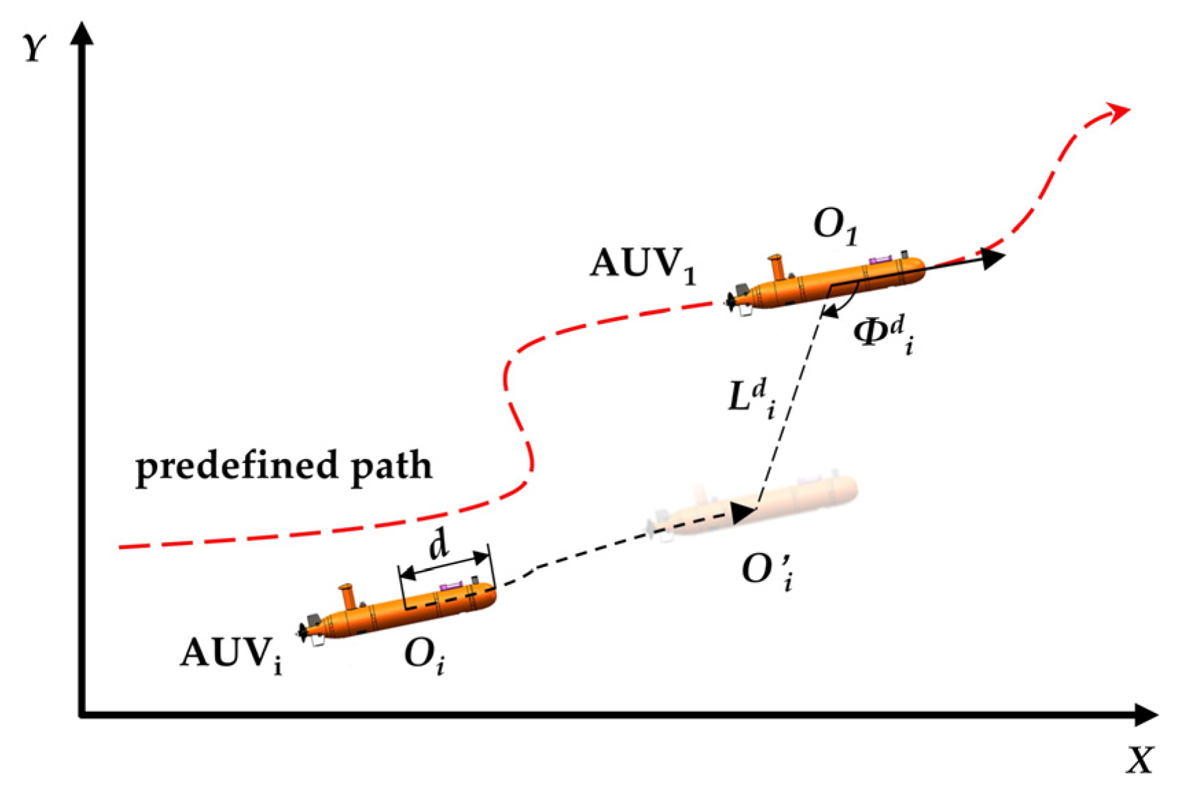
2.2. Description of Formation Control
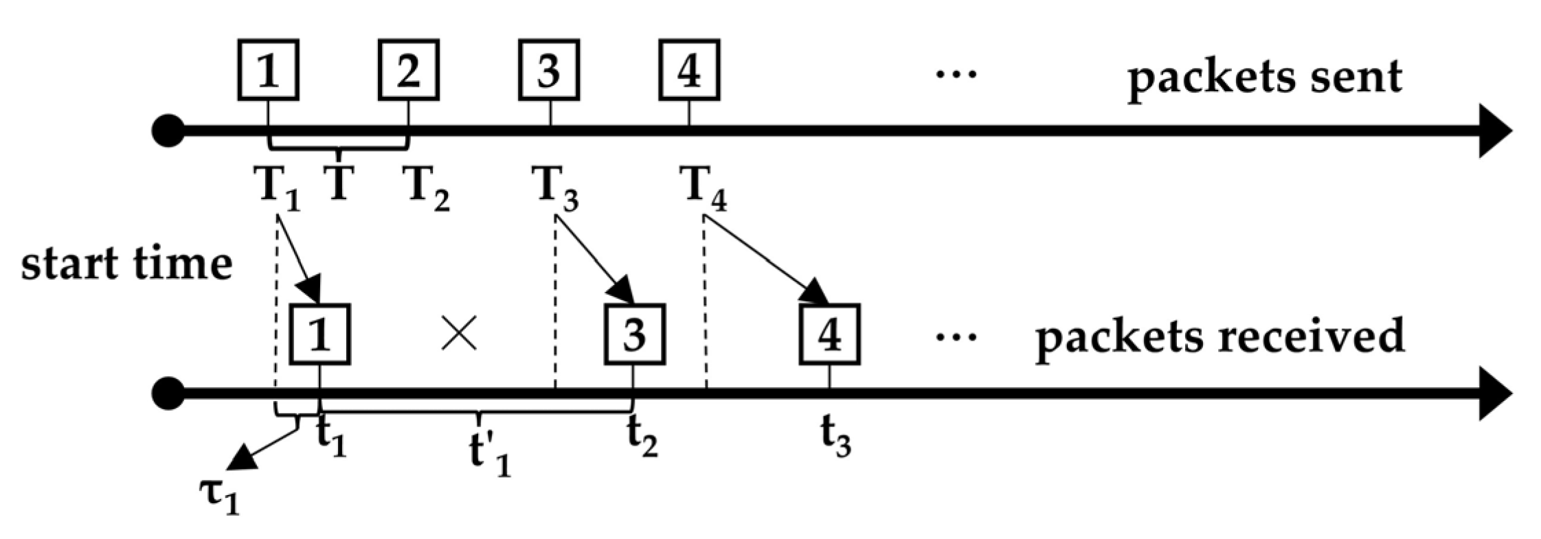
3. Solutions of Communication Delay, Packet Discreteness and Dropout
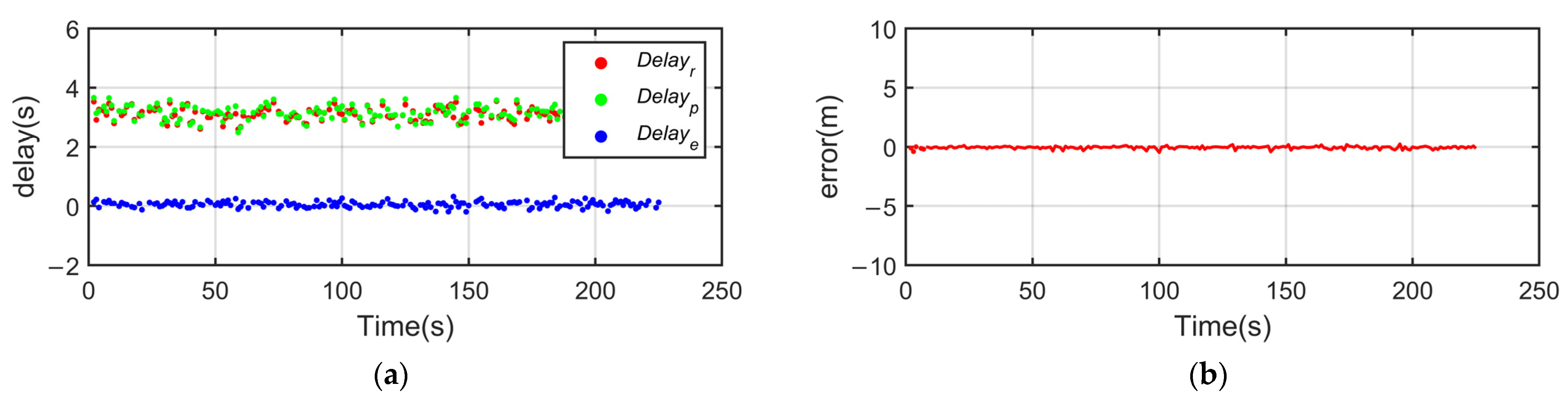
3.1. Estimation of Communication Delay
3.2. Prediction of Leader States
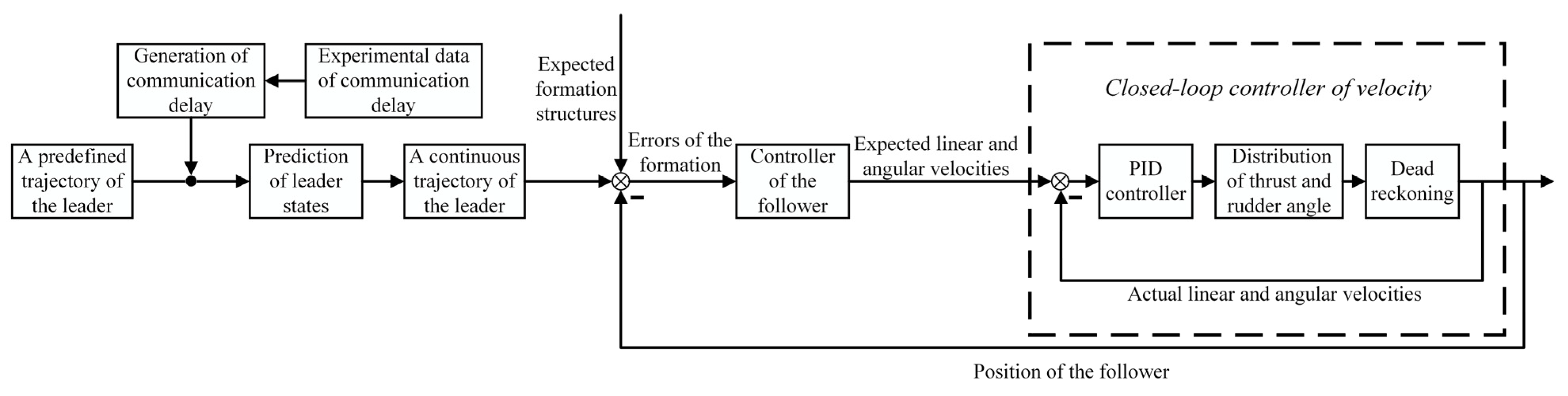
4. Formation Control Scheme
4.1. Generate Continuous Trajectories of the Leader
| Algorithm 1. Continuous Trajectories of the Leader |
| 1: The followers receive packets from the leader |
2: if 3: if, where denotes the time 4: then we obtain the communication delay using Equation (17) and the states of the leader are corrected 5: 7: then continuous trajectories of the leader are predicted 8: |
9: else 10: if 11: then we obtain the communication delay using Equation (17) and the states of the leader are corrected 12: 14: then and are updated using Equation (20) and the continuous trajectories of the leader are predicted according to Equations (21) and (22) 15: end |
4.2. Design the Follower Controller
5. Simulation Results
5.1. Simulation Environment
- Experimental methods
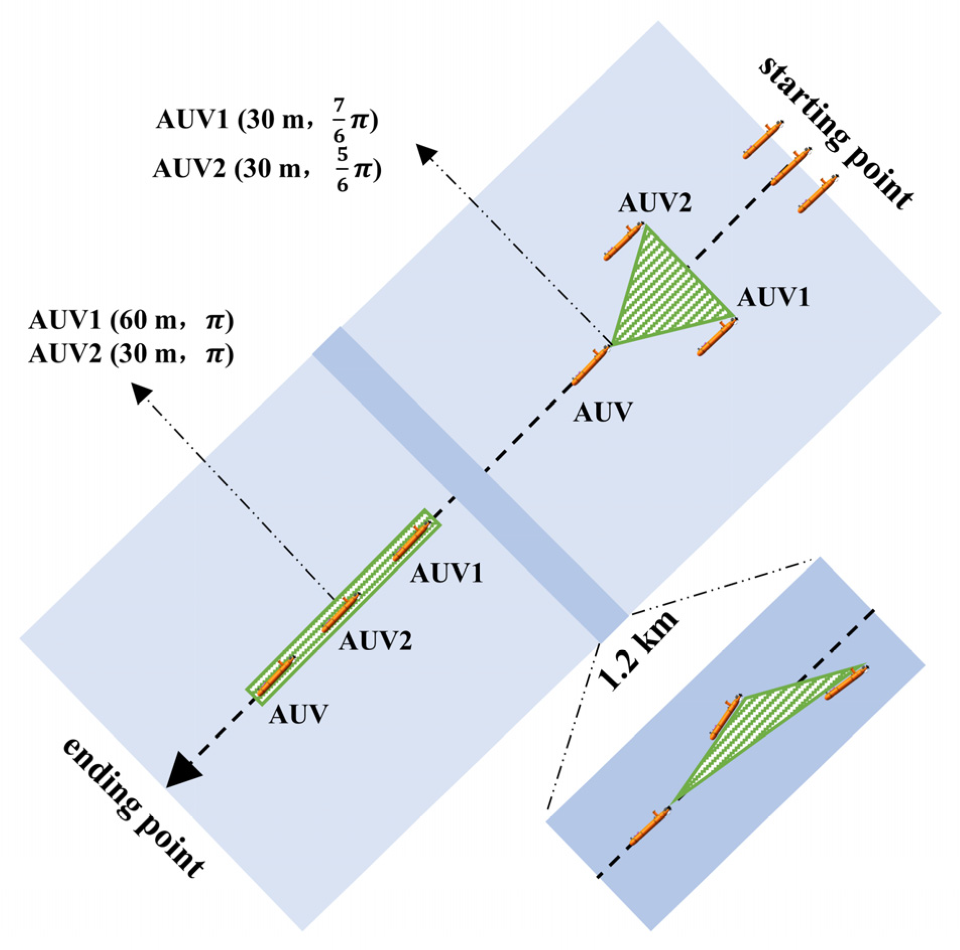
- Experimental scenario
- Communication environments
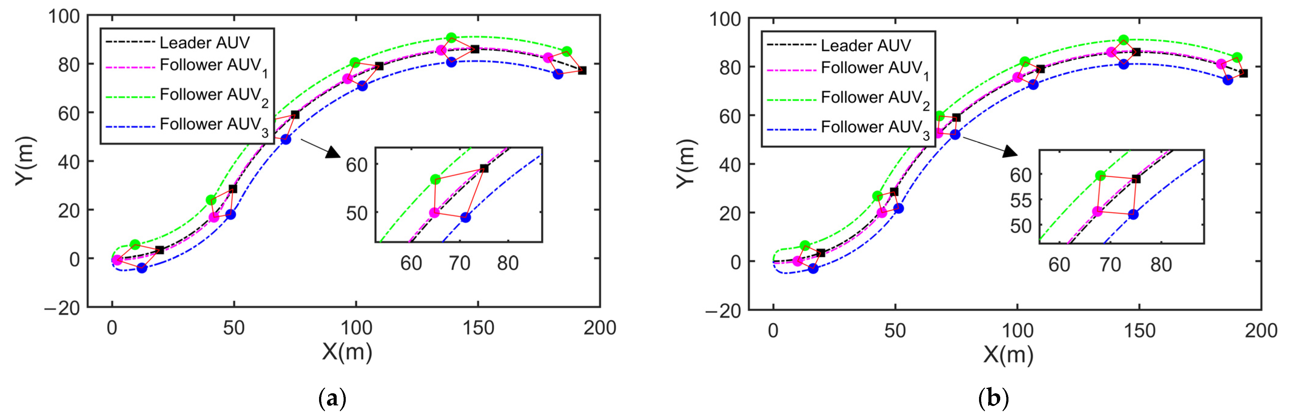
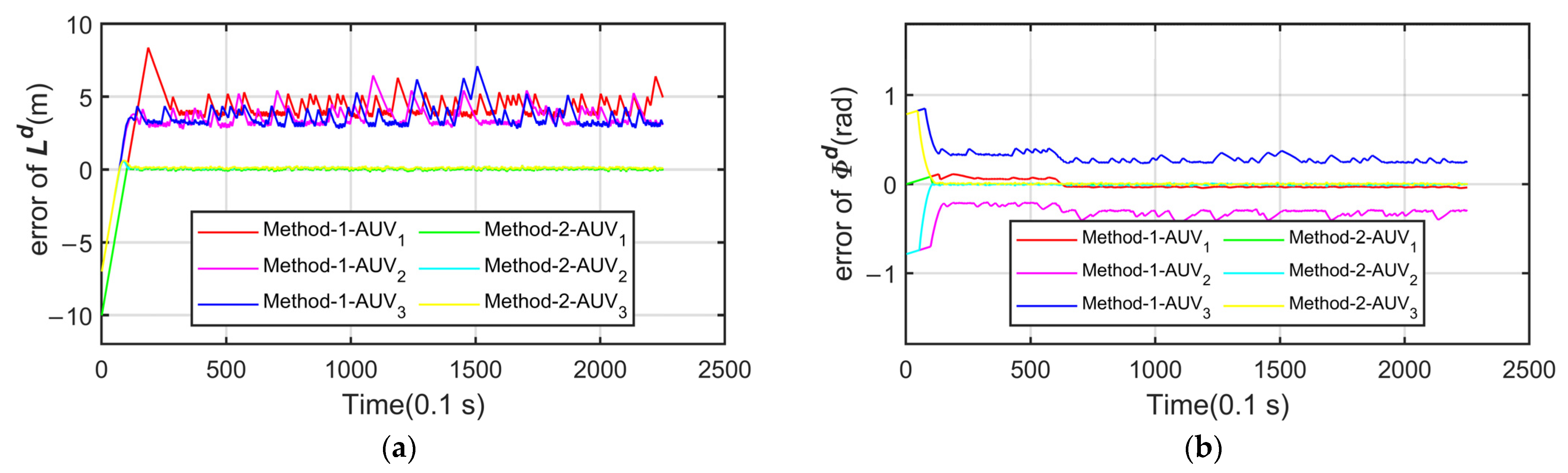
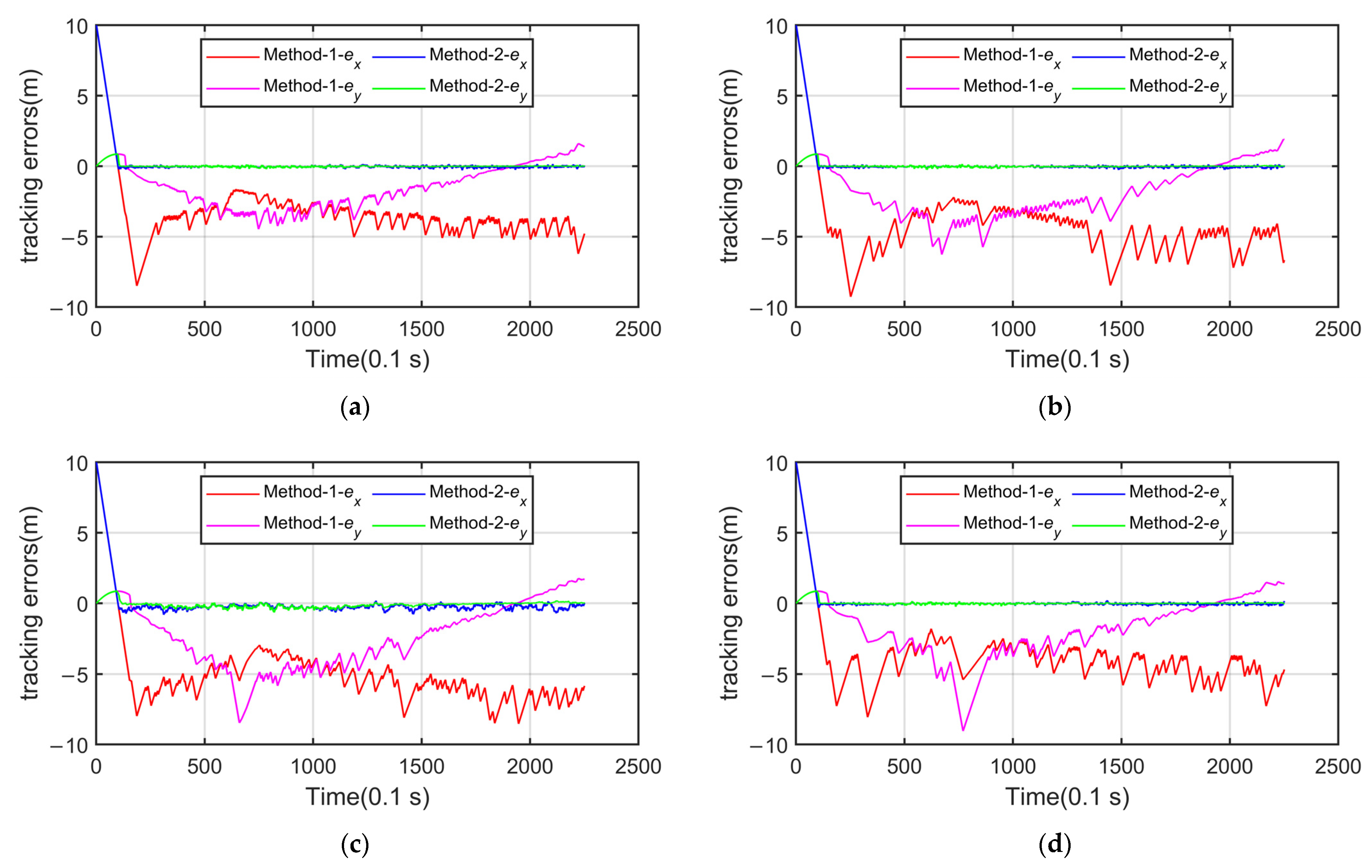
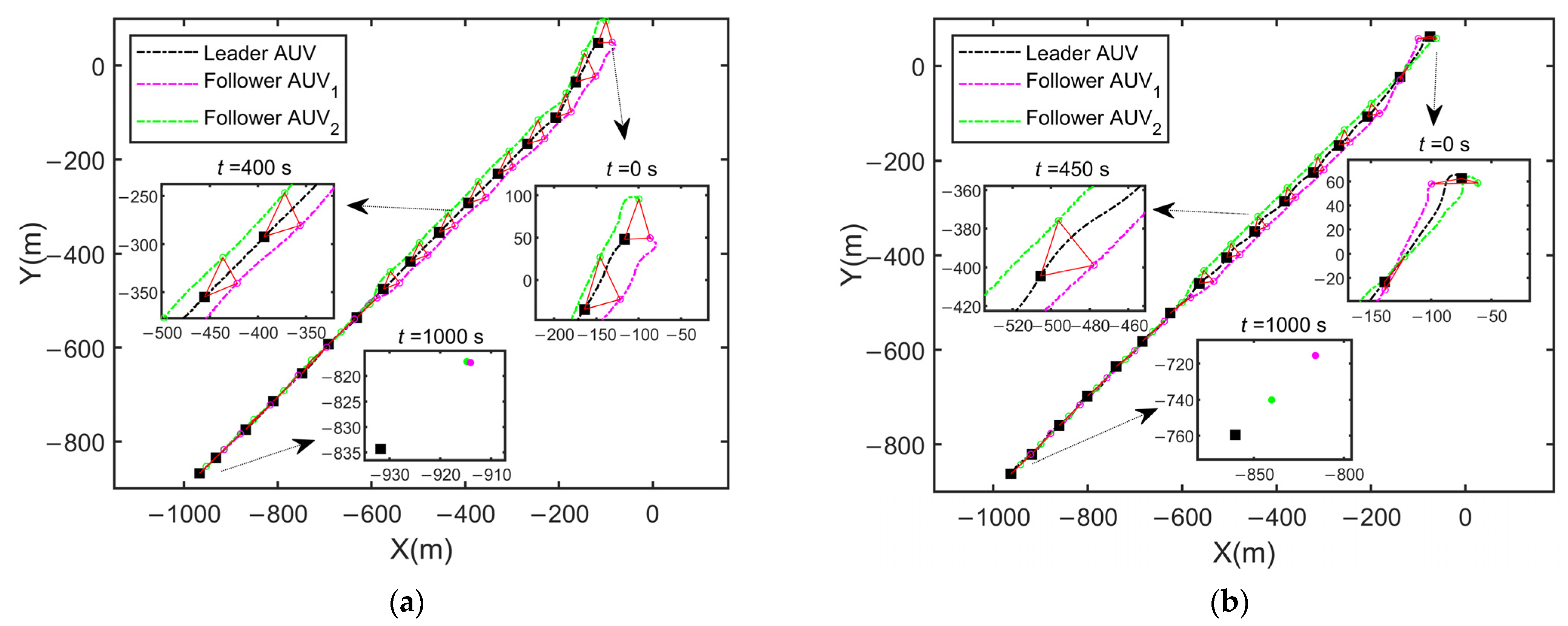
5.2. Simulation Results and Discussion
6. Field Tests
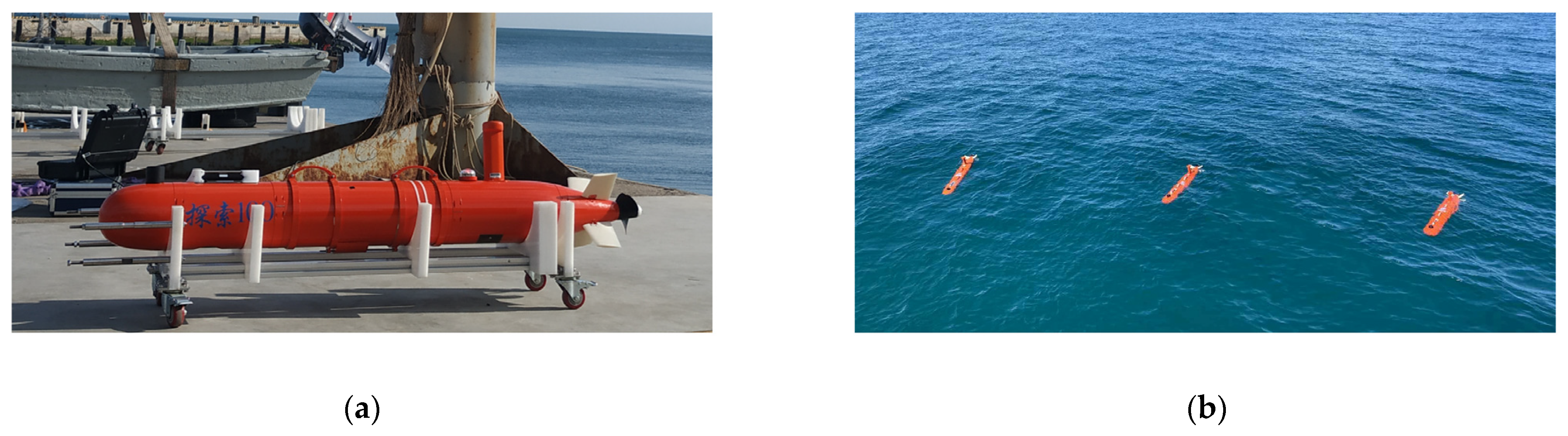
6.1. Vehicle Characteristics
6.2. Preparation and Scenario
6.3. Test Results and Discussion
7. Conclusions
Author Contributions
Funding
Institutional Review Board Statement
Informed Consent Statement
Data Availability Statement
Conflicts of Interest
References
- Nad, D.; Mandic, F.; Miskovic, N. Using Autonomous Underwater Vehicles for Diver Tracking and Navigation Aiding. J. Mar. Sci. Eng. 2020, 8, 413. [Google Scholar] [CrossRef]
- Pierdomenico, M.; Guida, V.G.; Macelloni, L.; Chiocci, F.L.; Rona, P.A.; Scranton, M.I.; Asper, V.; Diercks, A. Sedimentary facies, geomorphic features and habitat distribution at the Hudson Canyon head from AUV multibeam data. Deep-Sea Res. Part II-Top. Stud. Oceanogr. 2015, 121, 112–125. [Google Scholar] [CrossRef]
- Hwang, J.; Bose, N.; Nguyen, H.D.; Williams, G. Acoustic Search and Detection of Oil Plumes Using an Autonomous Underwater Vehicle. J. Mar. Sci. Eng. 2020, 8, 618. [Google Scholar] [CrossRef]
- Song, Y.; He, B.; Liu, P. Real-Time Object Detection for AUVs Using Self-Cascaded Convolutional Neural Networks. IEEE J. Ocean. Eng. 2021, 46, 56–67. [Google Scholar] [CrossRef]
- Martin-Abadal, M.; Pinar-Molina, M.; Martorell-Torres, A.; Oliver-Codina, G.; Gonzalez-Cid, Y. Underwater Pipe and Valve 3D Recognition Using Deep Learning Segmentation. J. Mar. Sci. Eng. 2021, 9, 5. [Google Scholar] [CrossRef]
- Zhang, Y.W.; Bellingham, J.G.; Ryan, J.P.; Kieft, B.; Stanway, M.J. Autonomous Four-Dimensional Mapping and Tracking of a Coastal Upwelling Front by an Autonomous Underwater Vehicle. J. Field Robot. 2016, 33, 67–81. [Google Scholar] [CrossRef] [Green Version]
- Feng, H.; Yu, J.C.; Huang, Y.; Qiao, J.A.; Wang, Z.Y.; Xie, Z.B.; Liu, K. Adaptive coverage sampling of thermocline with an autonomous underwater vehicle. Ocean Eng. 2021, 233, 109151. [Google Scholar] [CrossRef]
- Mao, Y.B.; Gao, F.R.; Zhang, Q.Z.; Yang, Z.Y. An AUV Target-Tracking Method Combining Imitation Learning and Deep Reinforcement Learning. J. Mar. Sci. Eng. 2022, 10, 383. [Google Scholar] [CrossRef]
- Das, B.; Subudhi, B.; Pati Bibhuti, B. Cooperative Formation Control of Autonomous Underwater Vehicles: An Overview. Int. J. Autom. Comput. 2016, 13, 199–225. [Google Scholar] [CrossRef]
- Zhang, L.-c.; Wang, J.; Wang, T.; Liu, M.; Gao, J. Optimal Formation of Multiple Auvs Cooperative Localization Based on Virtual Structure. In Proceedings of the MTS/IEEE Oceans Conference, Monterey, CA, USA, 19–23 September 2016. [Google Scholar] [CrossRef]
- Zhen, Q.; Wan, L.; Li, Y.; Jiang, D. Formation control of a multi-AUVs system based on virtual structure and artificial potential field on SE(3). Ocean Eng. 2022, 253, 111148. [Google Scholar] [CrossRef]
- Chen, G.; Shen, Y.; Qu, N.; He, B. Path planning of AUV during diving process based on behavioral decision-making. Ocean Eng. 2021, 234, 109073. [Google Scholar] [CrossRef]
- Xia, G.; Zhang, Y.; Zhang, W.; Zhang, K.; Yang, H. Robust adaptive super-twisting sliding mode formation controller for homing of multi-underactuated AUV recovery system with uncertainties. ISA Trans. 2022. [Google Scholar] [CrossRef] [PubMed]
- Li, Y.; Li, X.; Zhu, D.; Yang, S.X. Self-Competition Leader-Follower Multi-Auv Formation Control Based on Improved Pso Algorithm with Energy Consumption Allocation. Int. J. Robot. Autom. 2022, 37, 288–301. [Google Scholar] [CrossRef]
- Chen, B.; Hu, J.; Zhao, Y.; Ghosh, B.K. Finite-time observer based tracking control of uncertain heterogeneous underwater vehicles using adaptive sliding mode approach. Neurocomputing 2022, 481, 322–332. [Google Scholar] [CrossRef]
- Zhang, Y.; Wang, X.; Wang, S.; Tian, X. Three-dimensional formation-containment control of underactuated AUVs with heterogeneous uncertain dynamics and system constraints. Ocean Eng. 2021, 238, 109661. [Google Scholar] [CrossRef]
- Xia, G.; Zhang, Y.; Zhang, W.; Chen, X.; Yang, H. Dual closed-loop robust adaptive fast integral terminal sliding mode formation finite-time control for multi-underactuated AUV system in three dimensional space. Ocean Eng. 2021, 233, 108903. [Google Scholar] [CrossRef]
- Wang, Y.; Wang, Z.; Chen, M.; Kong, L. Pre define d-time sliding mode formation control for multiple autonomous un-derwater vehicles with uncertainties. Chaos Solitons Fractals 2021, 144, 110680. [Google Scholar] [CrossRef]
- Wang, C.; Cai, W.; Lu, J.; Ding, X.; Yang, J. Design, Modeling, Control, and Experiments for Multiple AUVs Formation. IEEE Trans. Autom. Sci. Eng. 2021, PP, 1–12. [Google Scholar] [CrossRef]
- Li, J.; Zhang, Y.; Li, W. Formation Control of a Multi-Autonomous Underwater Vehicle Event-Triggered Mechanism Based on the Hungarian Algorithm. Machines 2021, 9, 346. [Google Scholar] [CrossRef]
- Hou, S.P.; Cheah, C.C. Can a Simple Control Scheme Work for a Formation Control of Multiple Autonomous Underwater Vehicles? IEEE Trans. Control Syst. Technol. 2011, 19, 1090–1101. [Google Scholar] [CrossRef]
- Huang, X.; Li, Y.; Du, F.; Jin, S. Horizontal path following for underactuated AUV based on dynamic circle guidance. Robotica 2017, 35, 876–891. [Google Scholar] [CrossRef]
- Fabiani, F.; Fenucci, D.; Caiti, A. A distributed passivity approach to AUV teams control in cooperating potential games. Ocean Eng. 2018, 157, 152–163. [Google Scholar] [CrossRef]
- Yu, H.; Zeng, Z.; Guo, C. Coordinated Formation Control of Discrete-Time Autonomous Underwater Vehicles under Alterable Communication Topology with Time-Varying Delay. J. Mar. Sci. Eng. 2022, 10, 712. [Google Scholar] [CrossRef]
- Li, Y.P.; Yan, S.X. Formation Control of Multiple Autonomous Underwater Vehicles Based on State Feedback. In Proceedings of the 11th World Congress on Intelligent Control and Automation (WCICA), Shenyang, China, 29 June–4 July 2014; pp. 5523–5527. [Google Scholar]
- Stojanovic, M. Recent advances in high-speed underwater acoustic communications. IEEE J. Ocean. Eng. 1996, 21, 125–136. [Google Scholar] [CrossRef]
- Chitre, M.; Shahabudeen, S.; Stojanovic, M. Underwater acoustic communications and networking: Recent advances and future challenges. Mar. Technol. Soc. J. 2008, 42, 103–116. [Google Scholar] [CrossRef]
- Yang, G.; Dai, L.; Wei, Z.Q. Challenges, Threats, Security Issues and New Trends of Underwater Wireless Sensor Networks. Sensors 2018, 18, 3907. [Google Scholar] [CrossRef] [Green Version]
- Caiti, A.; Crisostomi, E.; Munafo, A. Physical Characterization of Acoustic Communication Channel Properties in Underwater Mobile Sensor Networks. In Proceedings of the 1st International ICST Conference on Sensor Systems and Software (S-CUBE 2009), Pisa, Italy, 7–9 September 2009; pp. 111–126. [Google Scholar]
- Ismail, A.S.; Wang, X.; Hawbani, A.; Alsamhi, S.; Aziz, S.A. Routing protocols classification for underwater wireless sensor networks based on localization and mobility. Wirel. Netw. 2022, 28, 797–826. [Google Scholar] [CrossRef]
- Farooq, M.U.; Wang, X.; Hawbani, A.; Khan, A.; Ahmed, A.; Alsamhi, S.; Qureshi, B. POWER: Probabilistic weight-based energy-efficient cluster routing for large-scale wireless sensor networks. J. Supercomput. 2022, 78, 12765–12791. [Google Scholar] [CrossRef]
- Wang, H.; Yemeni, Z.; Ismael, W.M.; Hawbani, A.; Alsamhi, S.H. A reliable and energy efficient dual prediction data re-duction approach for WSNs based on Kalman filter. IET Commun. 2021, 15, 2285–2299. [Google Scholar] [CrossRef]
- Suryendu, C.; Subudhi, B. Formation Control of Multiple Autonomous Underwater Vehicles Under Communication Delays. IEEE Trans. Circuits Syst. II-Express Briefs 2020, 67, 3182–3186. [Google Scholar] [CrossRef]
- Yang, H.Z.; Wang, C.F.; Zhang, F.M. A decoupled controller design approach for formation control of autonomous underwater vehicles with time delays. IET Control Theory Appl. 2013, 7, 1950–1958. [Google Scholar] [CrossRef]
- Yan, Z.P.; Yang, Z.W.; Yue, L.D.; Wang, L.; Jia, H.M.; Zhou, J.J. Discrete-time coordinated control of leader-following multiple AUVs under switching topologies and communication delays. Ocean Eng. 2019, 172, 361–372. [Google Scholar] [CrossRef]
- Chen, Y.; Guo, X.; Luo, G.; Liu, G. A Formation Control Method for AUV Group Under Communication Delay. Front. Bioeng. Biotechnol. 2022, 10, 848641. [Google Scholar] [CrossRef] [PubMed]
- Yan, Z.P.; Xu, D.; Chen, T.; Zhang, W.; Liu, Y.B. Leader-Follower Formation Control of UUVs with Model Uncertainties, Current Disturbances, and Unstable Communication. Sensors 2018, 18, 662. [Google Scholar] [CrossRef] [Green Version]
- Yan, Z.P.; Pan, X.L.; Yang, Z.W.; Yue, L.D. Formation Control of Leader-Following Multi-UUVs With Uncertain Factors and Time-Varying Delays. IEEE Access 2019, 7, 118792–118805. [Google Scholar] [CrossRef]
- Yang, Y.; Xiao, Y.; Li, T.S. A Survey of Autonomous Underwater Vehicle Formation: Performance, Formation Control, and Communication Capability. IEEE Commun. Surv. Tutor. 2021, 23, 815–841. [Google Scholar] [CrossRef]
- Millan, P.; Orihuela, L.; Jurado, I.; Rubio, F.R. Formation Control of Autonomous Underwater Vehicles Subject to Communication Delays. IEEE Trans. Control Syst. Technol. 2014, 22, 770–777. [Google Scholar] [CrossRef]
- Chen, K.; Luo, G.; Zhou, H.; Zhao, D. Research on Formation Control Method of Heterogeneous AUV Group under Event-Triggered Mechanism. Mathematics 2022, 10, 1373. [Google Scholar] [CrossRef]
- Wang, J.Q.; Wang, C.; Wei, Y.J.; Zhang, C.J. Filter-backstepping based neural adaptive formation control of leader-following multiple AUVs in three dimensional space. Ocean Eng. 2020, 201, 107150. [Google Scholar] [CrossRef]
- Chen, C.T.; Millero, F.J. Speed of Sound in Seawater at High-Pressures. J. Acoust. Soc. Am. 1977, 62, 1129–1135. [Google Scholar] [CrossRef]
- Dai, J.; Liu, Y.; Chen, J.; Liu, X. Fast feature selection for interval-valued data through kernel density estimation entropy. Int. J. Mach. Learn. Cybern. 2020, 11, 2607–2624. [Google Scholar] [CrossRef]
- Kim, J. Tracking Controllers to Chase a Target Using Multiple Autonomous Underwater Vehicles Measuring the Sound Emitted from the Target. IEEE Trans. Syst. Man Cybern. Syst. 2021, 51, 4579–4587. [Google Scholar] [CrossRef]
- Xia, G.; Zhang, Y.; Zhang, W.; Chen, X.; Yang, H. Multi-time-scale 3-D coordinated formation control for mul-ti-underactuated AUV with uncertainties: Design and stability analysis using singular perturbation methods. Ocean Eng. 2021, 230, 109053. [Google Scholar] [CrossRef]
- Wei, H.; Shen, C.; Shi, Y. Distributed Lyapunov-Based Model Predictive Formation Tracking Control for Autonomous Un-derwater Vehicles Subject to Disturbances. IEEE Trans. Syst. Man Cybern. Syst. 2021, 51, 5198–5208. [Google Scholar] [CrossRef]
- Su, B.; Wang, H.; Wang, Y.; Gao, J. Fixed-time Formation of AUVs with Disturbance via Event-triggered Control. Int. J. Control Autom. Syst. 2021, 19, 1505–1518. [Google Scholar] [CrossRef]
- Kim, J.H.; Yoo, S.J. Distributed event-driven adaptive three-dimensional formation tracking of networked autonomous underwater vehicles with unknown nonlinearities. Ocean Eng. 2021, 233, 109069. [Google Scholar] [CrossRef]
- Liu, H.; Wang, Y.; Lewis, F.L. Robust Distributed Formation Controller Design for a Group of Unmanned Underwater Ve-hicles. IEEE Trans. Syst. Man Cybern. Syst. 2021, 51, 1215–1223. [Google Scholar] [CrossRef]


| Parameter | Leader AUV | Follower AUV1 | Follower AUV2 | Follower AUV3 |
|---|---|---|---|---|
| Starting point (x, y) | (0,0) | (0,0) | (0,0) | (0,0) |
| Yaw (rad) | ||||
| Linear velocity (m/s) | 1.0289 | none * | none | none |
| Yaw velocity (rad/s) | −0.0175 | none | none | none |
| ) | none | |||
| Maximum linear velocity (m/s) | 1.5433 | 1.5433 | 1.5433 | 1.5433 |
| Maximum yaw velocity (rad/s) | 0.1 | 0.1 | 0.1 | 0.1 |
| Parameter | Environment-1 | Environment-2 | Environment-3 | Environment-4 |
|---|---|---|---|---|
| Communication delay (s) | * | |||
| Interval of sent packets (s) | 1 | 2 | 1 | 1 |
| Packet dropout rate (%) | 20 | 20 | 20 | 40 |
| Parameter | Environment-1 | Environment-2 | Environment-3 | Environment-4 | Average |
|---|---|---|---|---|---|
| Errors of distance (m) | 3.902 | 4.988 | 5.754 | 4.658 | 4.826 |
| Errors of angle (rad) | 0.226 | 0.261 | 0.284 | 0.253 | 0.256 |
| Parameter | Environment-1 | Environment-2 | Environment-3 | Environment-4 | Average |
|---|---|---|---|---|---|
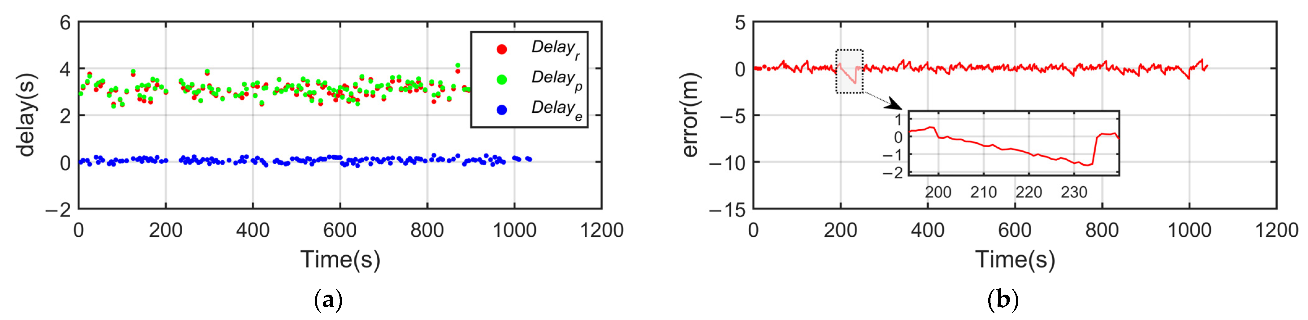
| Errors of estimated communication delay (s) | 0.092 | 0.095 | 0.087 | 0.098 | 0.093 |
| Errors of the prediction of the leader states (m) | 0.239 | 0.236 | 0.277 | 0.232 | 0.246 |
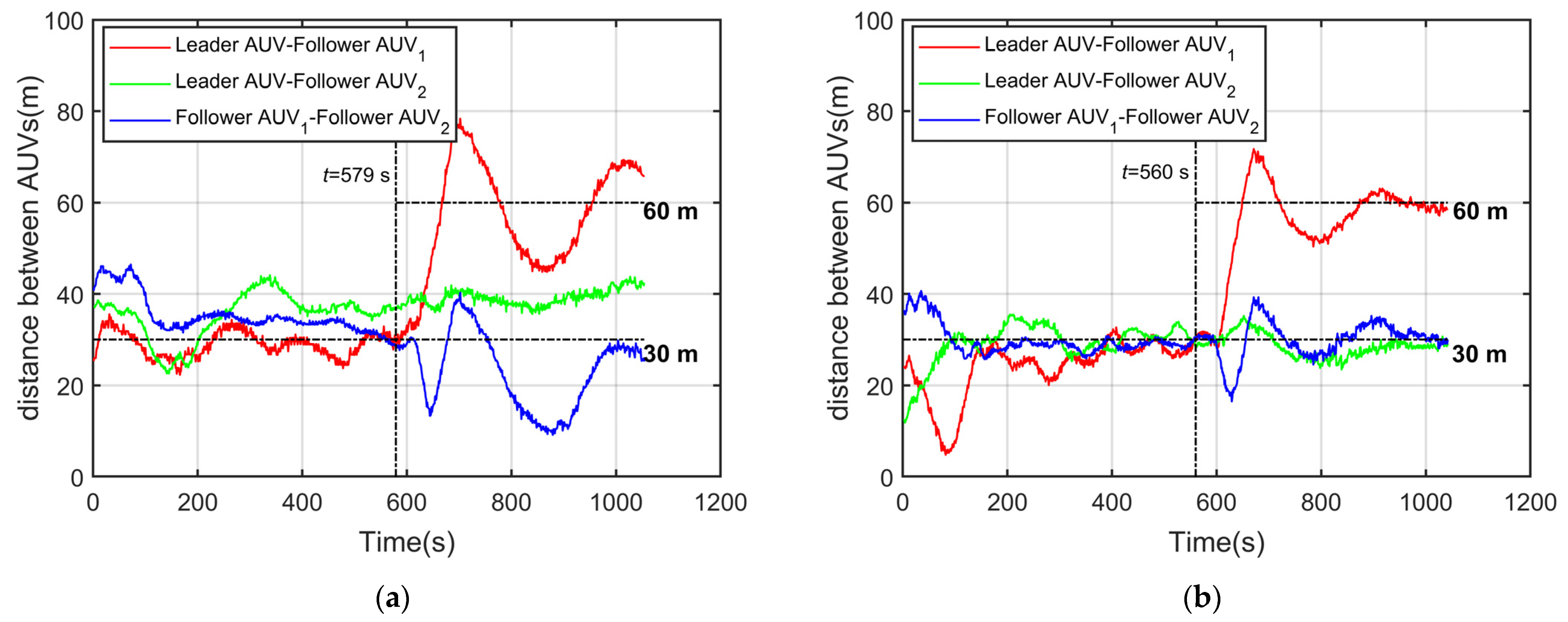
| Errors of distance (m) | 0.242 | 0.234 | 0.283 | 0.251 | 0.216 |
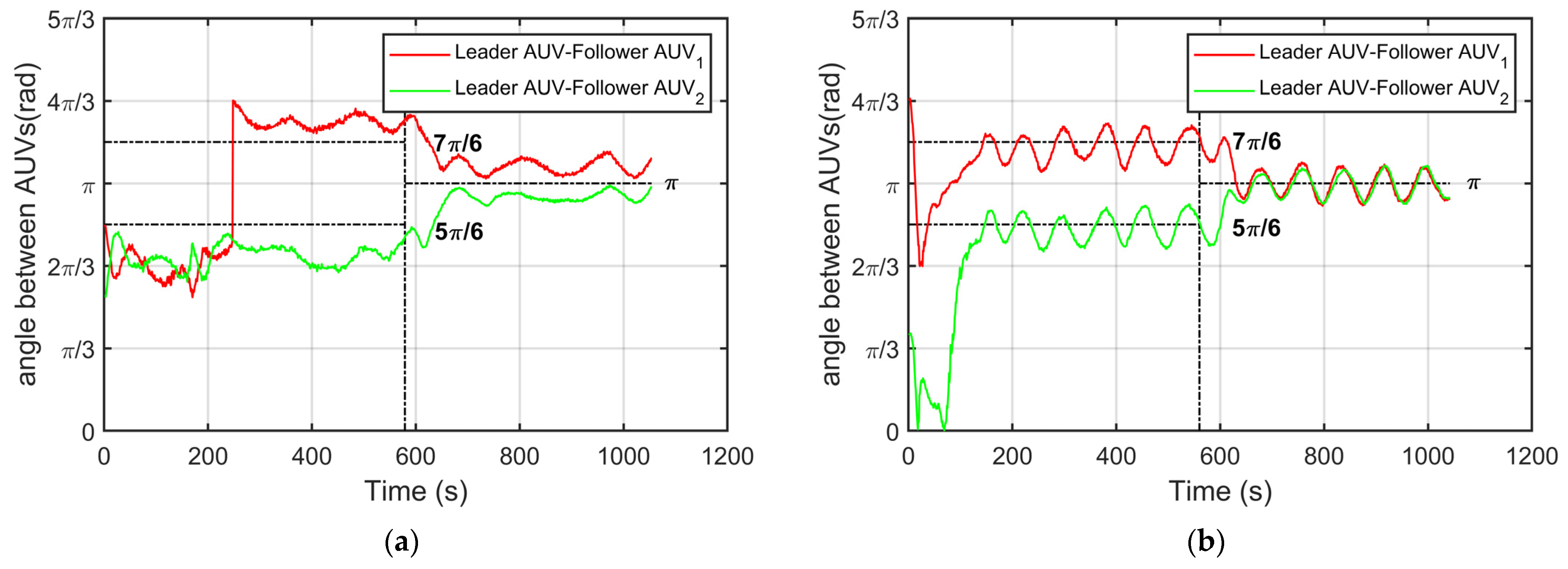
| Errors of angle (rad) | 0.021 | 0.022 | 0.026 | 0.021 | 0.023 |
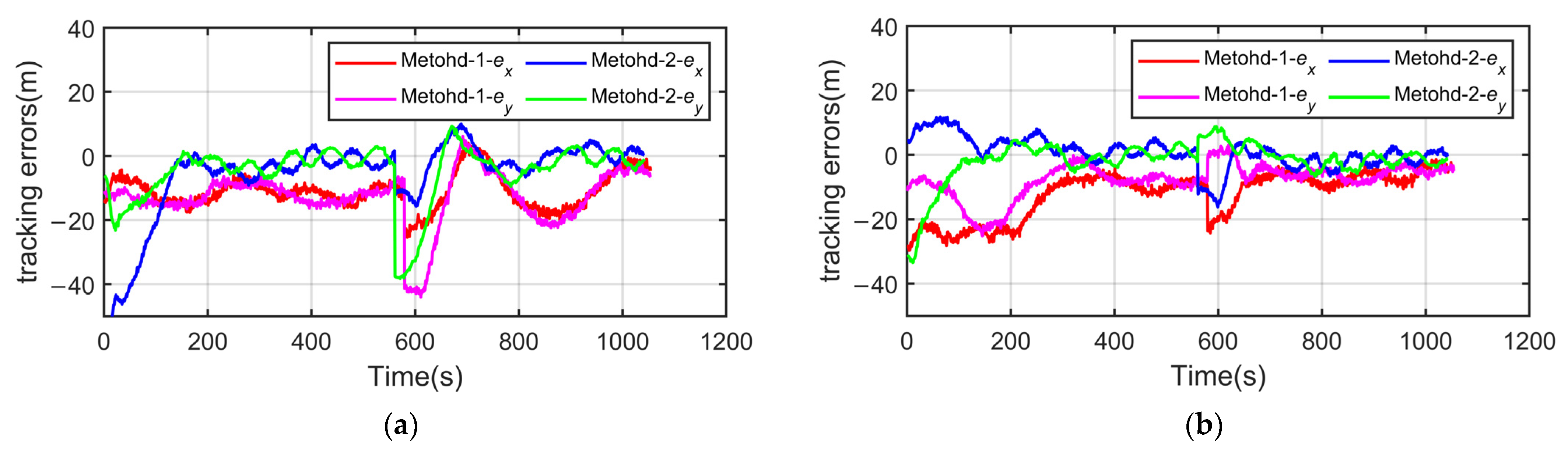
| Parameter | Method-1 | Method-2 | Method-3 | Method -4 |
|---|---|---|---|---|
| Errors of distance (m) | 4.826 | 0.216 | 2.137 | 2.695 |
| Errors of angle (rad) | 0.256 | 0.023 | 0.152 | 0.169 |
| Parameter | Test-1 | Test-2 | Test-3 | Test-4 | Average |
|---|---|---|---|---|---|
| Packet dropout rate (%) | 31.3 | 32.4 | 31.8 | 31.1 | 31.5 |
| Errors of distance (m) | 12.204 | 11.989 | 12.221 | 12.187 | 12.150 |
| Errors of angle (rad) | 0.408 | 0.419 | 0.412 | 0.399 | 0.410 |
| Parameter | Test-1 | Test-2 | Test-3 | Test-4 | Average |
|---|---|---|---|---|---|
| Packet dropout rate (%) | 33.1 | 31.2 | 30.5 | 32.3 | 31.8 |
| Errors of estimated communication delay (s) | 0.103 | 0.092 | 0.096 | 0.108 | 0.998 |
| Errors of the prediction of the leader states (m) | 0.833 | 1.142 | 0.986 | 1.048 | 1.002 |
| Errors of distance (m) | 5.453 | 5.398 | 5.429 | 5.364 | 5.411 |
| Errors of angle (rad) | 0.218 | 0.205 | 0.211 | 0.196 | 0.208 |
Publisher’s Note: MDPI stays neutral with regard to jurisdictional claims in published maps and institutional affiliations. |
© 2022 by the authors. Licensee MDPI, Basel, Switzerland. This article is an open access article distributed under the terms and conditions of the Creative Commons Attribution (CC BY) license (https://creativecommons.org/licenses/by/4.0/).
Share and Cite
Li, L.; Li, Y.; Zhang, Y.; Xu, G.; Zeng, J.; Feng, X. Formation Control of Multiple Autonomous Underwater Vehicles under Communication Delay, Packet Discreteness and Dropout. J. Mar. Sci. Eng. 2022, 10, 920. https://doi.org/10.3390/jmse10070920
Li L, Li Y, Zhang Y, Xu G, Zeng J, Feng X. Formation Control of Multiple Autonomous Underwater Vehicles under Communication Delay, Packet Discreteness and Dropout. Journal of Marine Science and Engineering. 2022; 10(7):920. https://doi.org/10.3390/jmse10070920
Chicago/Turabian StyleLi, Liang, Yiping Li, Yuexing Zhang, Gaopeng Xu, Junbao Zeng, and Xisheng Feng. 2022. "Formation Control of Multiple Autonomous Underwater Vehicles under Communication Delay, Packet Discreteness and Dropout" Journal of Marine Science and Engineering 10, no. 7: 920. https://doi.org/10.3390/jmse10070920