Integration of Node Classification in Storm Surge Surrogate Modeling

Abstract

Surrogate models, also referenced as metamodels, have emerged as attractive data-driven, predictive models for storm surge estimation. They are calibrated based on an existing database of synthetic storm simulations and can provide fast-to-compute approximations of the expected storm surge, replacing the numerical model that was used to establish this database. This paper discusses specifically the development of a kriging metamodel for the prediction of peak storm surges. For nearshore nodes that have remained dry in some of the synthetic storm simulations, a necessary first step, before the metamodel calibration, is the imputation of the database to address the missing data corresponding to such dry instances to estimate the so-called pseudo-surge. This imputation is typically performed using a geospatial interpolation technique, with the k nearest-neighbor (kNN) interpolation being the one chosen for this purpose in this paper. The pseudo-surge estimates obtained from such an imputation may lead to an erroneous classification for some instances, with nodes classified as inundated (pseudo-surge greater than the node elevation), even though they were actually dry. The integration of a secondary node classification surrogate model was recently proposed to address the challenges associated with such erroneous information. This contribution further examines the above integration and offers several advances. The benefits of implementing the secondary surrogate model are carefully examined across nodes with different characteristics, revealing important trends for the necessity of integrating the classifier in the surge predictions. Additionally, the combination of the two surrogate models using a probabilistic characterization of the node classification, instead of a deterministic one, is considered. The synthetic storm database used to illustrate the surrogate model advances corresponds to 645 synthetic tropical cyclones (TCs) developed for a flood study in the Louisiana region. The fact that various flood protective measures are present in the region creates interesting scenarios with respect to the groups of nodes that remain dry for some storms behind these protected zones. Advances in the kNN interpolation methodology, used for the geospatial imputation, are also presented to address these unique features, considering the connectivity of nodes within the hydrodynamic simulation model.

1. Introduction

The use of surrogate models (also referenced as emulators or metamodels) and machine learning techniques has gained increasing popularity for coastal hazard assessment applications [1,2,3,4,5,6,7,8,9,10]. These approaches represent data-driven predictive tools that are calibrated using a database of synthetic storm simulations, with the ultimate goal to establish fast-to-compute emulators that approximate (emulate) the expected storm surge with high accuracy. The output of the emulator is the storm surge (peak values or time-history evolution), and the input is the parametric features that can be used to uniquely describe each storm within the available database, for example, the parameters of the storm wind-field model. The emulator ultimately establishes an approximation of the input/output relationship and, when properly calibrated, can replace the high-fidelity numerical model utilized to develop the original synthetic storm database, offering predictions with similar accuracy and vastly improved computational efficiency. This circumvents any computational challenges associated with using the aforementioned high fidelity numerical models for real-time forecasting and storm surge risk assessment, ultimately allowing the development of efficient and versatile hazard prediction tools for emergency response management and regional planning [11,12]. Gaussian process emulators (kriging) have been proven in several studies [2,3,4,13,14,15] to offer great versatility as a surrogate modeling technique in this context, providing highly accurate storm surge predictions over large coastal regions with thousands of nodes and for databases of various sizes (number of storms) and characteristics (underlying features of the synthetic storms).

Given a database of synthetic storms, two essential steps are needed before the emulator calibration. These steps correspond, respectively, to the establishment of the input and output (observations) training data. First, a parameterization of the database is needed to define a vector of storm features that will serve as the emulator input. These features typically pertain to track, size, and intensity characteristics for each storm, and in order to account for the time evolution of these characteristics, different approaches can be established leading to a definition based on: (i) a specific reference instance (landfall or reference landfall for bypassing storm) [3], (ii) averaged values over some time-window around such a reference instance [16], or (iii) a description that considers the entire functional dependence over time [9,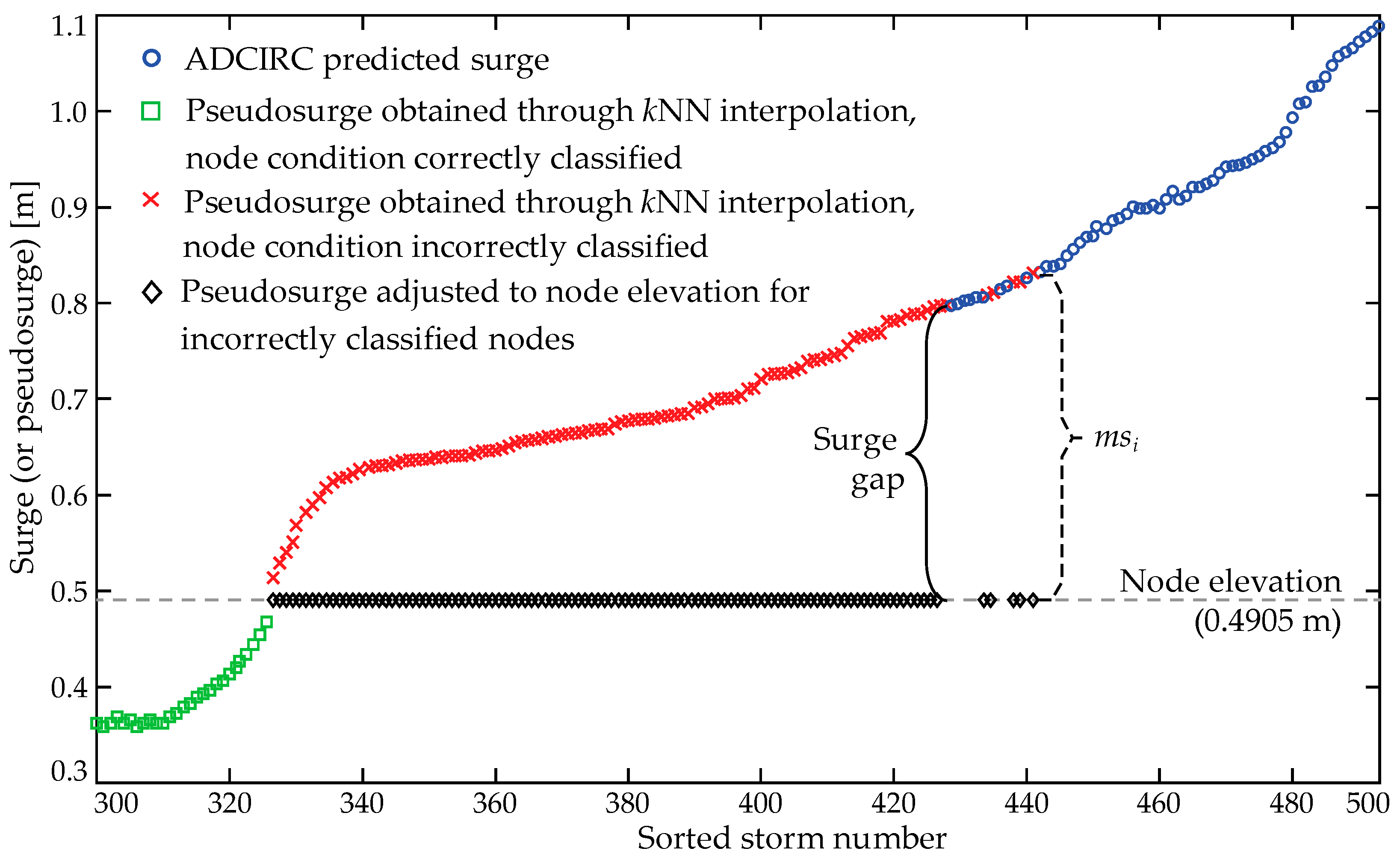17]. Second, for nearshore or onshore nodes that have remained dry in some of the synthetic storm simulations, the imputation of the database to address the missing data corresponding to such dry instances is warranted. This imputation process provides the pseudo-surge [18], which then replaces the missing data in the original database. Though both steps are important, the emphasis of this paper is on the second step, the database imputation.

Geospatial interpolation techniques, such as kriging [14] or k nearest-neighbor (kNN) interpolation [16] have been proven as appropriate for performing this imputation, leveraging the spatial correlation between nodes in order to infer missing data based on the surge values of other inundated nodes in close proximity. The selection of the exact type of geospatial interpolation depends on the number of nodes for which surge data is available, whether they correspond to the original numerical grid, which may include hundreds of thousands of nodes, or to some selected, few (up to a couple of thousand) save points. In the former case, a weighted kNN interpolation [16] has been shown to provide good accuracy and computational efficiency, whereas for the latter case, advanced geospatial interpolation techniques, such as kriging, can be explored [14] since the smaller size of the database (smaller number of nodes) does not pose insurmountable computational challenges for such techniques. Independently of the approach adopted to perform the imputation, the established pseudo-surge estimates may provide an erroneous classification for some storms, with the node classified as inundated based on the pseudo-surge (pseudo-surge value larger than node elevation), even though it is known, based on the original database, that the node is actually dry. Some adjustment of the imputed pseudo-surge is required for such instances, since the direct use of the erroneous pseudo-surge training data will ultimately lead to a poor emulator performance, over-predicting surge values for such cases. On the other hand, the type of this adjustment is also important since it can generate gaps in the input/output data, as demonstrated later, impacting the emulator calibration process and its predictive capabilities.

This paper examines this specific problem of appropriately adjusting the imputed pseudo-surge values for the accurate, emulator-based prediction of peak storm surge. The integration of a secondary node classification surrogate model was recently proposed [16] to address the challenges associated with the erroneous pseudo-surge values generated at the imputation stage. The proposed secondary surrogate model couples logistic principal component analysis (LPCA) [19] with a kriging emulator on the resultant natural parameters of the logistic process to establish an efficient classifier, even for applications with a large number of nodes. For any node that has been misclassified at least once during the database imputation, termed as a problematic node, the final surge predictions are established by combining the predictions of the secondary classification surrogate model and the primary storm surge surrogate model, which is established using the imputed database. It was recommended in [16] to adopt the predictions of the secondary classification surrogate when the primary surrogate provides the condition of the problematic node to be as inundated (surge estimate larger than the node elevation), in order to counteract the propensity of the latter to overestimate the surge. This contribution considers a number of critical advances for integrating such a node classification setting in storm surge surrogate modeling. The accuracy established from this integration is examined for groups of nodes with different characteristics, instead of averaging over the entire geographical domain, providing an in-depth analysis of the benefits that such an integration can offer and of the cases for which such benefits are critical for coastal hazard assessment. A detailed comparison to an alternative implementation, considering the direct adjustment of any erroneous pseudo-surge imputations, is also considered. Furthermore, potential advantages of combining the two different surrogates (node classification and surge prediction) are discussed across all nodes, without constraining only to the problematic ones. Finally, the probabilistic characterization of the node classification (condition), instead of a deterministic one, is examined for the surrogate model combination. This probabilistic characterization for the secondary surrogate model is facilitated directly using the underlying logistic regression, while for the primary surrogate model, it is developed utilizing the uncertainty quantification offered by the corresponding Gaussian process emulator. All these advances are illustrated using a 645 synthetic tropical cyclones (TCs) database developed for a flood study in the Louisiana region. Various flood protective measures are present in the region, creating interesting scenarios with respect to the group of nodes that remain dry behind them for many of the database storms. Some adjustments in the kNN interpolation used for the geospatial imputation are also discussed, considering the node grid connectivity within the hydrodynamic surge simulation model when deciding on the selection of the neighboring grid point locations, rather than basing any decisions solely on the closest distance. The development of different surge surrogate models for parts of the database with different surge behavior is also incentivized and investigated through some of the examined comparisons.

The remaining of the paper is organized as follows: Section 2 establishes the notation formalism used in this manuscript, with Section 3 presenting an overview of the database used in this study. Section 4 reviews the kNN imputation process and motivates the need to consider the node classification surrogate model. Section 5 reviews the fundamentals of the primary and secondary surrogate model developments, while Section 6 discusses details of the combination of the two surrogate models, distinguishing between different approaches based on the node characteristics at the database imputation stage. Finally, Section 7 considers a detailed presentation of results from the application of the combined surrogate model implementation to the Louisiana case-study database.

2. Notation Formalism

A database of n synthetic storms is available that provides surge predictions for a total of $n_z$ nodes within the computational domain. For the surrogate model development, each of the synthetic storms is parameterized through the $n_x$-dimensional vector $x\in {ℝ}^{n_x}$, which will serve as the emulator input, with $x_i$ denoting the ith input component. Further details on the selection of x for the case study database will be provided in Section 3. The input vector for the hth storm will be denoted as $x^h$. Let $z_i^h$ denote the peak surge for the ith node and the hth storm. Notation $z_i(x)$ will also be used for the surge of the ith node when the explicit dependence on the storm input vector needs to be highlighted. Let $z\in {ℝ}^{n_z}$ denote the $n_z$-dimensional surge vector, with its components corresponding to the surge values for all individual nodes of interest. All notations, including the subscript, superscript, and input dependencies, extend to the vector notation z as well. For example, $z^h=z(x^h)$ corresponds to the vector of peak surge for all nodes for the hth storm, which is described through the input vector $x^h$. The classification of the ith node condition for the hth storm is denoted by $I_i^h$ or $I_i(x^h)$ when the dependence on the storm input needs to be explicitly noted, with the convention that $I_i(x^h)=1$ corresponds to the node being inundated (wet) and $I_i(x^h)=0$ to the node being dry. The dry instances $I_i^h=0$ correspond to missing data in the original database, with no predictions for the corresponding storm surge $z_i^h$. The nodes for which $I_i^h$ is equal to 1 across all storms correspond to nodes that have been inundated across the entire database and will be referenced as “always wet” nodes, whereas the inland nodes for which $I_i^h$ is equal to 0 for at least one storm will be referenced as “once dry” nodes. The latter node group has at least one missing value (the surge is not provided for at least one storm) across the suite of storms. The number of at least once dry nodes will be denoted as $n_r$. Additionally, let the elevation of the ith node be $e_i$, and for each node define the surge gap as:

$${\eta }_i={\min }_h(z_i^h)-e_i$$

(1)

where ${\min }_h(.)$ denotes the minimum of the quantity inside the parentheses across all the storms in the database. The surge gap will be used later on to distinguish the dry nodes into different groups.

Finally, assembling the data across all storms, let X, Z, and $I^t$ denote the matrices for the storm input, surge, and node classification, respectively, whose rows correspond to the characteristics for individual storms. Across the manuscript, lower case variables denote characteristics for specific storms, and upper case variables refer to characteristics across the entire database. Matrix X has dimension $n\times n_x$, with rows corresponding to $x^h$; Z has dimension $n\times n_z$, with rows corresponding to $z^h$; and $I^t$ has dimension $n\times n_z$, with the $\{h,i\}$ element (hth row and ith column) corresponding to $I_i^h$. The instances/elements in matrix $I^t$ that correspond to value 0 represent the missing data in the original Z matrix. The database for the peak storm surge ultimately provides the parametric input matrix X and the peak surge matrix Z. The classification matrix $I^t$ is derived based on Z, with 0 representing instances of missing surge values (node is dry) and 1 the rest (node is inundated, so surge prediction is available).

3. Louisiana Database Overview

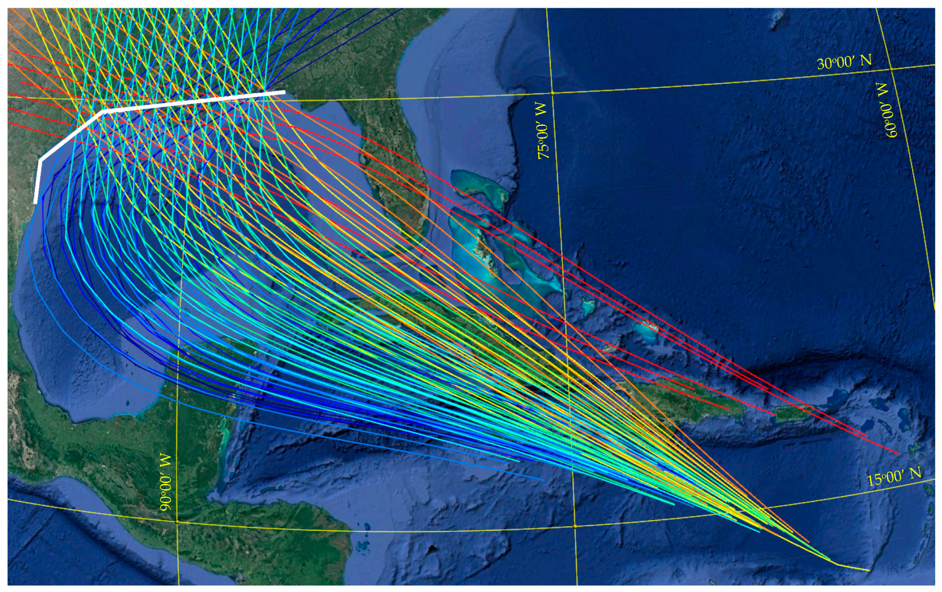
The database used in this study is part of the U.S. Army Corps of Engineers’ (USACE) Coastal Hazards System (CHS; https://chs.erdc.dren.mil (accessed on 15 April 2022)) [12]. The CHS Louisiana Coastal Study (CHS-LA) was conducted for quantifying storm hazards and coastal compound flooding in Louisiana, including areas in the vicinity of the Greater New Orleans Hurricane Storm Damage Risk Reduction System (HSDRRS). The storm suite developed for CHS-LA consists of n = 645 synthetic tropical cyclones (TCs), separated into eight main tracks, referenced herein as master tracks (MTs), as shown in Figure 1 and Figure 2. The grouping of the different tracks is based on the storm heading direction at the final approach before landfall. Figure 1 shows all unique storm tracks, separated into the MTs based on color, whereas Figure 2 presents separately the tracks within each MT, additionally establishing a magnification closer to landfall. All storms are characterized by unique combinations of the following parameters: landfall location, defined by the latitude, $x_{lat}$, and longitude of the storm track, $x_{lon}$; heading direction during final approach to landfall, β; central pressure deficit, $\Delta P$; translational speed, $v_t$; and radius of maximum wind speed, $R_{mw}$. The heading direction (β) dictates the MT (as shown in each of the subplots in Figure 2), and the combination of latitude $(x_{lat})$ and longitude $(x_{lon})$ the specific track within each MT. The remaining parameters dictate the strength $(\Delta P)$, size $(R_{mw})$, and speed $(v_t)$ characteristics of each synthetic storm, further distinguishing storms that might correspond to the same track. These characteristics have been held relatively constant prior to landfall, as shown in Figure 3, illustrating the variation of these storm parameters for a typical storm of the database.

Table 1. Characteristics of the database per master track (MT).

MT ID	Storm Heading β (°)	Number of Different Tracks (Landfall Locations)	Number of Storms per MT	Storm Parameter Range
				$\mathsf{\Delta }\mathit{P}$ (mbar)	${\mathit{R}}_{\mathit{m}\mathit{w}}$ (km)	${\mathit{v}}_{\mathit{t}}$ (m/s)
1	−80	6	48	[8 148]	[9.3 115.5]	[2.4 10.60]
2	−60	9	70	[18 138]	[11.8 127.5]	[2.4 12.50]
3	−40	13	104	[8 148]	[8.5 133.1]	[2.2 13.9]
4	−20	15	105	[18 138]	[9.1 116.5]	[2.4 11.80]
5	0	15	120	[8 148]	[8.0 130.0]	[2.4 13.05]
6	20	14	98	[18 138]	[8.6 138.2]	[2.3 12.65]
7	40	9	72	[8 148]	[9.6 141.3]	[2.3 12.85]
8	60	4	28	[18 138]	[9.4 119.4]	[2.5 13.4]

summarizes the range of the TC parameters that constitute the database. The reported values for each parameter correspond to the ones of peak storm intensity in each case.

The simulation of the 645 synthetic TCs in the CHS-LA database was performed using high-resolution, high-fidelity atmospheric and hydrodynamic numerical models. The parameters of the synthetic TC suite were first used as input to drive a Planetary Boundary Layer (PBL) model on a nested grid to generate the wind and pressure fields used as forcing in the hydrodynamic modeling. The hydrodynamic simulations were performed by coupling the ADCIRC (Advanced Circulation) model [20] and the SWAN (Simulating Waves Nearshore) wave model [21]. The ADCIRC mesh grid, corresponding to the v14a grid including the 2023 update of the coastal protection systems for the greater Louisiana region, consists of close to 1.6 million nodes and 3.1 million triangular elements. A subset of the entire domain will be considered for the metamodel development, focusing on areas around New Orleans, constrained by latitude (28.5°, 40°) N and longitude (86°, 93.5°) W. This corresponds to a total of $n_z=$1,179,179 nodes, with $n_r=$488,216 being dry in at least one storm. Figure 4 presents the dry/wet information for nodes and storms using histograms of (a) the percentage of storms that each node is inundated for, and of (b) the percentage of nodes that are inundated for each storm. Both histograms are presented as relative frequency plots, with the total number of elements per bin divided by the total number of elements, which is n_z for part (a) and n for part (b). Note that for part (a) of Figure 4, percentage equal to 1 corresponds to the always wet set.

The geographic domain includes various flood protection systems around the Greater New Orleans area. Within the ADCIRC numerical model, some of these systems were modeled using disconnected grids (no elements connecting nodes) with appropriate constraints across nodes to couple the water elevation.

Related to the storm parameterization, the characteristics at landfall are chosen to define x, taking into account the aforementioned small variability of the size, intensity, and speed along the synthetic storm track (demonstrated in detail in Figure 3). This leads to an input vector that includes the latitude, $x_{lat}$, and longitude, $x_{lon}$, for reference landfall; the heading direction for the storm MT, β; the central pressure deficit, $\Delta P$; the radius of maximum winds, $R_{mw}$; and the translational speed, $v_t$: $x=[x_{lat} x_{lon} \beta \Delta P R_{mw} v_t]$.

A simplified, piece-wise linear coastal boundary is utilized for defining the reference landfall, also shown in Figure 1 (white solid line). The boundary simplification is chosen based on the recommendations in [14] to avoid any ambiguous definition of landfall due to the existence of bays. The input parameters $x_{lat}$ and $x_{lon}$ are defined when the synthetic storm track crosses this boundary.

4. Dry node Imputation and Identification of the Challenges Associated with the Pseudo-Surge Estimates

This section describes the database imputation process, in order to estimate the pseudo-surge values, and discusses the challenges associated with erroneous classification based on such estimates.

4.1. Imputation Using Weighted kNN with ADCIRC Connectivity

A weighted kNN interpolation is adopted for the surge imputation, utilizing the same formulation as in [16]. The proximity of the nodes in the ADCIRC grid, also shown in subplot (a) of Figure 5, promotes high accuracy for the kNN interpolation in this setting, since neighboring nodes are short distances from one another, accommodating reliable predictions based on information from only the closest neighbors. Let $d_{ij}$ denote the geo-distance between nodes i and j and $A_k^h[i]$ the set of k closest nodes to the ith node for the hth storm, based on the calculated $d_{ij}$. Only nodes with known surge values are included in set $A_k^h[i]$; these may correspond to inundated nodes for the hth storm (nodes for which $I_i^h=1$), or to nodes with already imputed values within the iterative formulation discussed next. The ADCIRC connectivity can be incorporated using instead of the closest nodes based purely on $d_{ij}$, the closest connected nodes, where the latter is defined by the number of ADCIRC element edges between nodes i and j in the graph representing the ADCIRC numerical grid. Figure 5b illustrates this concept; for a specific node of interest (red dot), the one (magenta), two (yellow), and three (cyan) edge connectivity neighbors are shown. Evidently, nodes with a higher edge connectivity cannot be included in set $A_k^h[i]$ before all other neighbors with lower edge connectivity (irrespective of their distance) are included. This way, nodes that might appear close based on $d_{ij}$ but belong to different or disconnected sections of the ADCIRC grid, for example, due to the presence of bays and/or riverine systems (complex geomorphology) or due to flood protection systems, are not utilized in the kNN implementation.

Based on the information in set $A_k^h[i]$, the pseudo-surge estimate, ${\underset{˜}{z}}_i^h$, for the ith node and the hth storm based on the weighted kNN interpolation is given by:

$$\begin{array}{l}{\underset{˜}{z}}_i^h=\frac{{\displaystyle \sum _{j\in A_k^h[i]}w(d_{ij})z_j^h}}{{\displaystyle \sum _{j\in A_k^h[i]}w(d_{ij})}}\\ w(d_{ij})=\{\begin{array}{c}{e}^{-{\left(\frac{d_{ij}}{q}\right)}^p} \mathrm{if} d_{ij}<d\\ 0 \mathrm{if} d_{ij}\ge d\hfill \end{array}\hfill \end{array}$$

(2)

where $w(d_{ij})$ is a distance-dependent weight taken as a power exponential expression with parameters d, q, and p [16]. A cut-off distance d is introduced in the definition of weights $w(.)$ to avoid faraway nodes influencing the kNN interpolation in any irregular parts of the grid. The set of $[k d q p]$ parameters of Equation (2) corresponds to the hyper-parameters for the weighted kNN interpolation that need to be calibrated. This calibration can be performed using information for the wet nodes [16], a process briefly reviewed in Appendix A.

As suggested in [16], an iterative imputation can be adopted for each storm to better accommodate hydraulic connectivity. This iterative kNN implementation examines the imputation separately for each storm. At each iteration, the imputation is done only on dry nodes that have at least k wet (imputed and genuine) neighbors in a larger set of $k_c$ nodes. If fewer than k wet neighbors are available, no value is imputed in the current iteration. The value of $k_c$ is chosen equal to twice the value of k in this study, adopting the same recommendation as in [16]. This implementation facilitates a gradual, spatial imputation propagating surge values gradually from offshore to onshore nodes, mimicking the physical wetting process. The use of the ADCIRC connectivity in the nearest neighbor selection, discussed earlier, incorporates additional considerations of the hydraulic connectivity close to any zones with protection systems (i.e., disconnected parts of the grid).

4.2. Issues Related to Misclassification Based on the Pseudo-Surge

The kNN-based imputation is not guaranteed to lead to pseudo-surge values, ${\underset{˜}{z}}_i^h$, that are smaller than the node elevation, $e_i$, since no such constraint is explicitly enforced into the formulation. Nodes for which the imputed surge is projected to be higher than the node elevation are falsely classified as wet based on the pseudo-surge values. For addressing such erroneous information, two solutions can be considered [16]: (a) artificially modify the estimated pseudo-surge so that it is smaller than the node elevation (e.g., 5 cm below the node elevation, $e_i$), guaranteeing that the node is correctly classified even based on the pseudo-surge values; or (b) maintain the pseudo-surge values obtained directly through the geospatial imputation, but consider a classification surrogate model to provide predictions for the node condition based on the original database (condition classification matrix $I^t$) to address the erroneous information in the pseudo-surge database. The set of nodes that have been misclassified at least once during the imputation process will be denoted as $A_{mc}$ and will be referenced herein as problematic nodes. The number of those nodes will be denoted as $n_p$. The database corresponding to the imputed pseudo-surge with no modification (case (b)) will be referenced herein as “pseudo-surge database”, and the database with adjustments to guarantee that the pseudo-surge value is smaller than the node elevation will be referenced herein as “corrected pseudo-surge database”. Before moving forward, is it important to stress that, as discussed in the introduction, the pseudo-surge is introduced merely as a mean to support the surge metamodel development (imputation of missing values in the original database), and there is no correct value for it from a theoretical perspective [16]. Both the pseudo-surge database and corrected pseudo-surge database should be deemed as possible alternatives for supporting the surge metamodel formulation, and the most appropriate one can be only evaluated based on the accuracy of that metamodel. It is important to view the subsequent discussions from this perspective.

Illustration of the challenges associated with some of the problematic nodes is facilitated through Figure 6, depicting the surge and pseudo-surge values for such a node across all the storms within the database. Note that a similar figure and relevant discussion were also included in [16] for this purpose. Here, this discussion is repeated for illustration clarity and in order to further motivate the need to address the falsely classified nodes, while establishing an additional connection to the surge gap defnition introduced in this paper. Specifically, this figure presents the pseudo-surge values obtained through the kNN-imputation in ascending order across the storms, and the node elevation with a horizontal line. Note that a portion of the entire database is shown, corresponding to pseudo-surge values close to the node elevation. The depicted blue circles correspond to surge predictions for the original database (node is inundated), while the green squares and the red × correspond to the kNN-based imputed pseudo-surge for the storms for which the node was originally dry. Green squares correspond to the correctly classified nodes with imputed surge below the node elevation, therefore still classifying the node as dry, while the red × to an erroneous classification, with the node classified as wet based on the imputed surge value. For the corrected pseudo-surge database approach, the erroneously classified values corresponding to the red × would have been mapped below the node elevation, as shown in Figure 6 with the black ×. This creates a discontinuity (“jump”) in the corrected pseudo-surge database for this specific node, which will create challenges for the subsequent surrogate model development. This jump corresponds to the surge gap, ${\eta }_i$, defined earlier in Equation (1). The larger the value of this gap, the greater the reduction of the prediction accuracy for any emulator, as such discontinuities in an otherwise smooth behavior (note the smooth characteristics across the remaining surge and pseudo-surge estimates in this figure) create significant challenges at the emulator calibration stage [22]. This is the motivation for using the pseudo-surge database; it is expected to accommodate the calibration of a higher accuracy surge surrogate model, provided that the secondary classification surrogate model can ultimately address the erroneous information (red × points) in the database.

For the case-study database, with $n_r$ = 488,216 nodes that required imputation for some of the storms, the misclassification statistics for the kNN-based imputation are the following: (i) when ADCIRC connectivity information is not utilized, then misclassification is 22.1%, whereas the set $A_{mc}$ of problematic nodes consists of $n_p$ = 322,753 nodes, and (ii) when ADCIRC connectivity is incorporated, then misclassification is 20.2%, whereas the set $A_{mc}$ of problematic nodes consists of n_p = 311,826 nodes. Minor differences are observed across the two examined variants.

Looking into more detail the characteristics of the problematic nodes for the case study, Figure 7 presents a histogram of the surge gap over their population. The number of nodes having surge gaps larger than 0.25, 0.5, 1, and 2 m are respectively 35,947, 16,504, 4290, and 267. Results indicate that a considerable number of nodes has larger values for the surge gap. Such values can be attributed to the existence of complex geomorphologies or flood protection systems, and are expected to reduce the predictive accuracy if the corrected pseudo-surge database is utilized, as indicated by the illustrative example in Figure 6.

Something that needs to be further considered in better assessing the challenges associated with the problematic nodes is the quality of information associated with these. Two different measures are introduced to quantify this. The first measure, denoted $m{s}_i$, is the maximum surge misinformation, defined as the difference between the largest pseudo-surge value among the instances the node was originally dry and the node elevation, given by:

$$m{s}_i={\max }_h\{({\underset{˜}{z}}_i^h-e_i)|I_i^h-1|\}$$

(3)

Note that the multiplication by $|I_i^h-1|$ is leveraged in the above equation to restrict the operation within the brackets (search for maximum in this case) to only the originally dry instances, corresponding to $I_i^h=0$. The maximum surge misinformation represents the largest magnitude of misclassification error. It is indicated in Figure 6 with a dashed line. The second measure, denoted as $m{p}_i$, is the percentage of misinformation, defined as the ratio of the number of instances (storms) a node has been misclassified at the kNN imputation stage over the total number of storms:

$$m{p}_i=\frac{{\displaystyle \sum _{h=1}^n}\{\mathbb{I}[{\underset{˜}{z}}_i^h>e]|I_i^h-1|\}}{n}$$

(4)

where $\mathbb{I}[.]$ denotes the indicator function, corresponding to one if the expression inside the brackets is true and to zero otherwise. The percentage of misinformation represents the amount of erroneous information for a problematic node. In Figure 6, this percentage is equivalent to the number of black crosses over the total number of storms. Small values for $m{s}_i$ and $m{p}_i$ indicate that even though a node has been misclassified at least once, both the magnitude and frequency of that misclassification are minimal. This is demonstrated clearly in Figure 8, where for both measures, a large number of nodes has very small $m{s}_i$ and $m{p}_i$ values. Consideration of such nodes, with both $m{s}_i$ and $m{p}_i$ values being very small, as problematic might not be an appropriate approach. This concept will be further investigated when the integration of the different surrogate models is examined later on in Section 6.

5. Review of the Surrogate Model Development

This section offers an overview of the two surrogate models: the primary one for predicting the storm surge $z_i(x^h)$, denoted as $S_s$ herein, and the secondary one for classifying the node condition $I_i(x^h)$, denoted as $S_c$ herein. Kriging is adopted for both as the metamodeling technique. However, the foundational ideas for combining the two models, as detailed in Section 6, can be applied to any type of surrogate model. Appendix B reviews the essential characteristics of the metamodel development. To accommodate the large dimensionality of the output vector (nodes of interest for estimating surge), some form of principal component analysis will be used for both types of surrogate models (classification and surge predictions).

5.1. Surrogate Model for Surge Predictions

The surrogate model for the surge prediction, $S_s$, uses the imputed database as observations for the metamodel calibration. Notation z (for individual storms) and Z (for the entire database across all storms) will be utilized to describe the observations, with the understanding that for any instance for which surge values are missing in the original database (node is dry), the missing $z_i^h$ is replaced by the pseudo-surge ${\underset{˜}{z}}_i^h$ for defining the observation matrix Z.

To improve the metamodel accuracy, some physics-motivated [8] or functional [16] transformation can be applied. The transformed surge for the ith node and the hth storm will be denoted as $z_i^t(x^h)$, with the transformed surge vector across all nodes denoted as $z^t$, and the corresponding transformed observation database as $Z^t$. The mathematical relationship between $z_i^t(x^h)$ and $z_i(x^h)$ will be denoted as $g(.)$ and is assumed to be invertible, with inverse $g^{-}{}^1(.)$. Without loss of generality, we will assume that $g(.)$ is strictly positive. This assumption is only relevant for the implementation of the probabilistic classification based on the $S_s$ surrogate. For the case study, the square root is employed as functional transformation, shown to be beneficial in past applications [16], leading to:

$$z_i^t=g(z_i)=\sqrt{z_i+c_i} \mathrm{and} z_i=g^{-1}(z_i^t)={(z_i^t)}^2-c_i$$

(5)

where $c_i$ is chosen equal to the minimum of $z_i$ over the storm database, but not greater than 0, and is utilized to make the argument under the square root positive across all storms.

The surrogate model is ultimately established, for the transformed surge $z^t$, with observation matrix $Z^t$. The detailed implementation is presented in [2,16]. Here only the basic steps are reviewed:

Step 1 (dimensionality reduction): Perform principal component analysis (PCA) as a dimensionality reduction technique to identify a smaller number of $m_s<n<<n_z$ latent outputs (principal components) $u\in {ℝ}^{m_s}$ through a linear projection. Individual components are distinguished through subscript j herein, with u_j denoting the jth element of vector u. The PCA is performed for the observation matrix $Z^t$ and provides the mean vector $\mu \in {ℝ}^{n_z}$, whose ith component ${\mu }_i$ corresponds to the mean of $\left\{z_i^t\right(x^h); h=1,\dots ,n\}$ (mean surge over the storm database for each node), the projection matrix $P\in {ℝ}^{n_z\times m_s}$, and for each latent component, $u_j$, the output vector of responses over the storm database $U_j(X)={[u_j(x^1) \dots u_j(x^n)]}^T\in {ℝ}^n$.

Step 2 (metamodel calibration): Develop $m_s$ separate surrogate models based on the procedure described in Appendix B for each of the principal components, setting $y=u_j$ and $Y\left(X\right)=U_j\left(X\right)$. Note that instead of developing individual surrogate models for each component, a grouping of the components may be considered as an alternative implementation to facilitate higher computational efficiency. Details for this formulation are included in [16].

Step 3 (metamodel predictions for the transformed surge): The surrogate model approximation for the transformed surge ${\tilde{z}}^t(x|X)$ is obtained by combining the predictions ${\tilde{u}}_j(x|X)$ for each of the $m_s$ latent outputs, given by Equation (A3) for the predictive mean and Equation (A4) for the predictive variance. Note that, as discussed in Appendix B, a functional dependence on the database X is utilized in our notation to accommodate the easier description of the cross-validation predictions used later in the manuscript. Using notation ${[.]}_{ij}$ to denote the $\{i,j\}\mathrm{th}$ element of a matrix (ith row and jth column), the kriging predictions (mean) for the ith node are:

$${\tilde{z}}_i^t(x|X)={\mu }_i+{\displaystyle \sum _{j=1}^{m_s}{[P]}_{ij}{\tilde{u}}_j(x|X)}$$

(6)

whereas the predictive variance is:

$${({\sigma }_i^t(x|X))}^2={\displaystyle \sum _{j=1}^{m_s}{[P]}_{ij}^2{\sigma }_j^2(x|X)}$$

(7)

Ultimately kriging establishes the following probabilistic model prediction: $z_i^t(x|X)~N({\tilde{z}}_i^t(x|X),{({\sigma }_i^t(x|X))}^2)$ [2,23], where N(a,b) stands for a Gaussian distribution with mean a and variance b. Though typically only the mean of this distribution is utilized, taken to represent the metamodel predictions, for certain aspects of the integration of the classification estimates that will be investigated in this manuscript, the use of the complete probabilistic description will be explored.

Step 4 (metamodel predictions for surge): Finally, the kriging predictions for the surge can be obtained by the transformation $g^{-1}(.)$:

$${\tilde{z}}_i(x|X)=g^{-1}({\tilde{z}}_i^t(x|X))={({\tilde{z}}_i^t(x|X))}^2-c_i$$

(8)

where the last equality in Equation (8) holds for the transformation utilized in the case study that follows. The classification of the node condition (wet or dry) based on the $S_s$ surrogate model is obtained by comparing the surge estimate to the node elevation. Denoting as $I_i^s(x|X)$ that classification for the ith node and for the storm with input x, we have:

$$I_i^s(x|X)=\mathbb{I}[{\tilde{z}}_i(x|X)>e_i]$$

(9)

where, as defined earlier, $\mathbb{I}[.]$ denotes the indicator function, corresponding to one if the expression inside the brackets is true and to zero otherwise.

As discussed in the introduction, for the combination of the predictions based on the two different surrogate models (discussed later in Section 6), the probabilistic characteristics of the classification will be examined. For the $S_s$ surrogate, these characteristics are accommodated by considering the Gaussian nature of the emulator. Let P[.] denote probability, and define as $p_i^s(x|X)$ the probability that the ith node is wet (inundated). Then based on the Gaussian distribution for $z_i^t(x|X)$, and assuming that $g(e_i)$ is well-defined, it is straightforward to show that:

$$p_i^s(x|X)=P[z_i(x|X)>e_i]=P[g(z_i(x|X))>g(e_i)]=\Phi \left[\frac{{\tilde{z}}_i^t(x|X)-g(e_i)}{{\sigma }_i^t(x|X)}\right]$$

(10)

where $\Phi [.]$ denotes the standard Gaussian cumulative distribution function and for the second equality the fact that $g(.)$ is strictly positive function was used. If $g(e_i)$ is not well-defined, for example if $e_i+c_i<0$ for the transformation of Equation (5), then the surge surrogate model will always lead in estimating $I_i^s(x|X)=p_i^s(x|X)=1$ (surge will never be predicted smaller than the node elevation). This probabilistic classification will be used (in Section 6) for nodes that have remained dry for some of the storms in the database, for which $e_i$ is expected to be positive, leading to a well-defined $g(e_i)$ for transformations like the one discussed in Equation (5). Alternatively, if the importance of establishing a probabilistic classification is greater than any benefits coming from utilizing the transformation $g(.)$, the use of the transformation itself can be omitted if it is deemed as problematic.

Finally, related to the selection of $m_s$ for the PCA, the following comments can be made. Typically, the first few principal components can be predicted well by the corresponding surrogate model, but the accuracy of higher components drastically reduces, leading to a saturation of the surrogate model accuracy as the number of principal components increases [2]. To establish a balance between accuracy and computational efficiency, especially with respect to memory requirements which are critical for real-time applications [11], a parametric analysis can be employed to investigate such benefits [14]. An alternative formulation was proposed in [16], considering only a small number of principal components and complementing the predictions with a surrogate model for the residuals. Such an implementation can also address any concerns related to overfitting stemming from the PCA application. In the case study considered in [16] it was shown that this approach could not offer any accuracy improvements, and since it increases the computational complexity of the overall $S_s$ implementation, it was suggested to be avoided. To provide an additional validation for this manuscript that treats a different database, this implementation that involves the residual surrogate will be briefly revisited later on.

5.2. Surrogate Model for Node Classification

The surrogate model for the node wet/dry classification, $S_c$, uses as observations the binary output $I_i(x^h)$ for near-shore nodes that have remained dry for some of the storms. Nodes that are inundated for all the storms are ignored in this classification problem, since they will always be predicted as inundated by a binary classifier. Additionally, the nodes considered for $S_c$ can be further reduced to correspond only to the problematic set $A_{mc}$. Let $A_c$ denote the set of $n_c$ nodes for which the classification surrogate model is considered (either nodes that were at least once dry or the problematic nodes). The observation matrix for the surrogate is denoted as $I^c$ and corresponds to the columns of $I^t$ matrix that belong in set $A_c$.

For the $S_c$ surrogate model, logistic principal component analysis (LPCA) [19] is used as the dimensionality reduction technique. LPCA also accommodates the transformation of the original categorical (binary) observations to continuous observations to facilitate the subsequent approximation through the kriging metamodel. The implementation is based on a multivariate generalization of the Bernoulli distribution, using the natural parameters (log-odds) θ and the canonical link function (logistic function). If ${\theta }_i(x^h)$ is the natural parameter for the ith node and the hth storm, then the probability of a node being wet is given by the logistic function:

$$P[I_i(x^h)=1|{\theta }_i(x^h)]=\frac{1}{1+e^{-{\theta }_i(x^h)}}$$

(11)

The dimensionality reduction is integrated into the process by considering a compact representation of the log-odds matrix $\Theta ={[\mathsf{\theta }(x^1) \dots \mathsf{\theta }(x^n)]}^T\in {ℝ}^{n\times n_c}$. This compact representation is expressed as $\Theta =T{V}^T+\Delta$, where T is the $n\times m_c$ matrix of coefficients, V is the $n_c\times m_c$ matrix of projection vectors, and Δ is a matrix with each row corresponding to the same bias vector ${\Delta }_{\theta }^T$ ($1\times n_c$ vector). This representation directly provides the latent space of logistic principal components t with observations T, as well as the projection matrix V and the bias vector Δ_θ to be used for the transformation from t tο θ, which takes the form:

$$\mathsf{\theta }(x)=Vt(x)+{\Delta }_{\theta }$$

(12)

The vector t ultimately provides the transformation to a continuous output with a significantly reduced dimension $m_c$ compared to the original categorical observations of dimension $n_c$.

LPCA is the integral first step in the $S_c$ formulation. Details for this formulation are presented in [16]. Here only the basic steps are reviewed:

Step 1 (dimensionality reduction and transformation of the predicted output): Using the observations $I^c$, perform LPCA for a chosen number of principal components $m_c$. This is established by maximizing the likelihood of observations $I^c$ given the compact representation of $\Theta$ for the natural parameters of the Bernoulli distribution [19], and ultimately provides the bias vector ${\Delta }_{\theta }^T$, the projection matrix V and the latent observation matrix T whose hth row corresponds to the latent output for the hth storm $t(x^h)$.

Step 2 (metamodel calibration): Develop $m_c$ separate surrogate models based on the procedure described in Appendix B for each of the principal components, setting y = t_j and $Y(X)=T_j(X)$, where $T_j(X)$ is the jth column of T. Similar to $S_s$, instead of developing individual surrogate models for each component, a grouping of the components may be considered to facilitate higher computational efficiency.

Step 3 (metamodel predictions for the natural parameters): The surrogate model approximation for the natural parameters $\tilde{\mathsf{\theta }}(x|X)$ is calculated by combining the predictions ${\tilde{t}}_j(x|X)$ for each of the $m_c$ latent outputs, obtained according to Equation (A3). Maintaining, as for $S_s$, the notation for the functional dependence on the database X, the predictions are:

$$\tilde{\mathsf{\theta }}(x|X)=V\tilde{t}(x|X)+{\Delta }_{\theta }^T$$

(13)

Step 4 (classification predictions): The probability of the ith node being wet for a specific storm input x according to the $S_c$ model, is given by the logistic function:

$$p_i^c(x|X)=P[I_i(x)=1|{\tilde{\theta }}_i(x|X)]=\frac{1}{1+e^{-{\tilde{\theta }}_i(x|X)}}$$

(14)

The deterministic classification prediction for node i according to surrogate model $S_c$ can then be established by comparing value $p_i^c$ to the 0.5 threshold. Denoting that prediction as $I_i^c(x^h|X)$, we have:

$$I_i^c(x|X)=\mathbb{I}[p_i^c(x|X)>0.5]$$

(15)

LPCA is known to be very prone to overfitting [24,25], a tendency that is exacerbated in the application examined here, since any additional overfitting originating from the metamodel calibration needs to be considered. For this reason, it was suggested in [16] to select $m_c$ in the first step of the $S_c$ formulation through a parametric sensitivity analysis, examining the metamodel accuracy through a cross-validation setting. Similarly to the $S_s$ surrogate model development, using a smaller $m_s$ and coupling it with a surrogate model on the residual predictions can be considered. Details for such an implementation are discussed in [16].

5.3. Metamodel Validation

Validation is important for obtaining a confidence metric for the surrogate model prediction accuracy, as well as for selecting the number of retained components for the PCA $(m_s)$ and LPCA $(m_c)$ implementations. Cross-validation (CV) is adopted as the validation approach here, implemented through the following steps: the storm database is partitioned into different groups; each group is sequentially removed from the database, and the remaining storms are used as observations to calibrate a surrogate model; this model is then used to make predictions for the surge of the removed storms; accuracy statistics are estimated comparing these predictions to the actual storm output. Details for the CV implementation and the utilized validation metrics are reviewed in the next two subsections.

5.3.1. Cross-Validation Implementation

The simplest CV approach is the leave-one-out cross-validation (LOOCV), established by removing sequentially a single storm at a time from the original database X. LOOCV is typically implemented without repeating the PCA/LPCA or the hyper-parameter calibration for each reduced database, since the opposite choice would substantially increase the computational complexity, requiring a total of n repetitions of the entire surrogate model calibration. This also allows the use of closed-form solutions [26] to obtain the leave-one-out (LOO) predictions without the need to explicitly remove each of the storms from the database. Computational details for the use of the closed-form solutions are included in [16]. As also discussed in [16], LOOCV cannot explore in depth any challenges associated with overfitting, since it does not repeat the PCA or LPCA implementations and the hyper-parameter calibration after the removal of each storm. This is especially important for examining the proper selection of the $m_c$ value for the LPCA implementation, since for other overfitting challenges (i.e., for the selection of $m_s$ for PCA or for the hyper-parameter calibration) minor impact has been shown in past studies. k-fold CV circumvents this problem by repeating both the PCA or LPCA and the hyper-parameter calibration, since in this case, depending on the number of groups that will be pre-defined, the re-calibration is not as expensive as in a LOOCV setting.

If $A_h$ is the subset containing the hth storm and $X_{-A_h}$ the remaining database, excluding set $A_h$, then repeating the surrogate model formulation starting with the observations corresponding to the set $X_{-A_h}$, provides, for the h^th storm the predictions ${\tilde{z}}_i(x^h|X_{-A_h})$ from the $S_s$ surrogate model and $p_i^c(x^h|X_{-A_h})$ from the $S_c$ surrogate model. Using these predictions, the node classification can also be obtained: $I_i^s(x^h|X_{-A_h})$ according to $S_s$ utilizing Equation (9) [using ${\tilde{z}}_i(x^h|X_{-A_h})$] and $I_i^c(x^h|X_{-A_h})$ according to $S_c$ utilizing Equation (15) [using $p_i^c(x^h|X_{-A_h})$]. Note that for the LOOCV implementation, only Step 3 of the formulation needs to be repeated, and in this case, closed-form solutions can be used for all predictions.

5.3.2. Validation Metrics

For the node condition classification, the adopted validation metric corresponds to the node misclassification percentage. If ${\tilde{I}}_i(x^h|X_{-A_h})$ are the CV-based metamodel predictions for the ith node condition and the hth storm, corresponding to $I_i^c(x^h|X_{-A_h})$ for the $S_c$ surrogate or to $I_i^s(x^h|X_{-A_h})$ for the $S_s$ surrogate, or to the $I_i^{cb}(x^h|X_{-A_h})$ for the combined formulation discussed in Section 6, then the total misclassification for this specific node and storm is given by:

$$M{C}_i^h=|{\tilde{I}}_i(x^h|X_{-A_h})-I_i(x^h)|$$

(16)

We can further distinguish between the false positive, i.e., node predicted wet when dry, and false negative, i.e., node predicted dry when wet, indicators, given respectively by:

$$\begin{array}{l}{}^{+}M{C}_i^h=\max (0,{\tilde{I}}_i(x^h|X_{-A_h})-I_i(x^h))\\ {}^{-}M{C}_i^h=\max (0,I_i(x^h)-{\tilde{I}}_i(x^h|X_{-A_h}))\end{array}$$

(17)

where max(a,b) is the function that provides the maximum of the two arguments a or b. Average statistics per node or across the entire database can then be obtained. For the total misclassification, these statistics are denoted as $M{C}_i$ and $\overline{MC}$, respectively, and are given by:

$$M{C}_i=\frac{1}{n}{\displaystyle \sum _{h=1}^{n}M{C}_i^h}; \overline{MC}=\frac{1}{n{n}_z}{\displaystyle \sum _{h=1}^n{\displaystyle \sum _{i=1}^{n_z}M{C}_i^h}}$$

(18)

Similar expressions as the two presented in Equation (18) hold for the false positive or the false negative misclassification definitions, with the only adjustment being that instead of averaging by $n_z$, the number of nodes that were dry (for the false positive misclassification) or wet (for the false negative misclassification) is utilized for each storm. Furthermore, statistics can be examined for specific groups instead of the entire node set, simply by considering the averaging in Equation (18) only for the specific nodes belonging to the group of interest (for indexes i corresponding to that group only).

For the surge predictions, both normalized and unnormalized statistics should be utilized. Unnormalized statistics reflect the absolute error, while normalized ones express the relative error, incorporating the response magnitude when assessing the size of the error. For normalized statistics, the correlation coefficient (cc) is adopted here. The correlation coefficient is unitless (as a normalized error metric), with values close to 1 indicating a better performance. For the ith node it is expressed by:

$$c{c}_i=\frac{\frac{1}{n}{\displaystyle \sum _{h=1}^n\left({\tilde{z}}_i(x^h|X_{-A_h})-\frac{1}{n}{\displaystyle \sum _{h=1}^n{\tilde{z}}_i(x^h|X_{-A_h})}\right)\left(z_i(x^h)-\frac{1}{n}{\displaystyle \sum _{h=1}^n{z}_i(x^h)}\right)}}{\sqrt{\frac{1}{n}{\displaystyle \sum _{h=1}^n{\left({\tilde{z}}_i(x^h|X_{-A_h})-\frac{1}{n}{\displaystyle \sum _{h=1}^n{\tilde{z}}_i(x^h|X_{-A_h})}\right)}^2}}\sqrt{\frac{1}{n}{\displaystyle \sum _{h=1}^n{\left(z_i(x^h)-\frac{1}{n}{\displaystyle \sum _{h=1}^n{z}_i(x^h)}\right)}^2}}}$$

(19)

Similar to the misclassification metric presented above, the overall metamodel accuracy is quantified by the averaged error statistics across all output locations, given by:

$$\overline{cc}=\frac{1}{n_z}{\displaystyle \sum _{i=1}^{n_z}c{c}_i}$$

(20)

Common candidates for unnormalized statistics include measures like the absolute mean error or the mean squared error. An alternative option, and the one chosen here, is the surge score [15,18], which for the ith node and the hth storm is described as:

$$S{C}_i^h=\{\begin{array}{c}|{\tilde{z}}_i(x^h|X_{-A_h})-z_i(x^h)|\\ {\tilde{z}}_i(x^h|X_{-A_h})-e_i\\ z_i(x^h)-e_i\\ 0\end{array}\begin{array}{c} \mathrm{if} {\tilde{I}}_i(x^h|X_{-A_h})=1 \& I_i(x^h)=1 \\ \mathrm{if} {\tilde{I}}_i(x^h|X_{-A_h})=1 \& I_i(x^h)=0\\ \mathrm{if} {\tilde{I}}_i(x^h|X_{-A_h})=0 \& I_i(x^h)=1\\ \mathrm{if} {\tilde{I}}_i(x^h|X_{-A_h})=0 \& I_i(x^h)=0\end{array}$$

(21)

This surge score shares the units of surge (unnormalized) and provides a penalty function for the discrepancy between the predicted and actual surge, further incorporating the node classification: (i) if a node is predicted wet and it is actually wet, then the absolute value of the predicted surge discrepancy is used as a penalty function; (ii) if a node is predicted wet, but it is dry, then the difference between predicted surge and node elevation is used as a penalty; (iii) if a node is predicted dry, but it is wet, then the difference between the actual surge and the node elevation is used as a penalty; (iv) if a node is predicted dry and it is dry, then penalty is zero. The averaged statistics per node or across the entire database can be then obtained, respectively, as:

$$S{C}_i=\frac{1}{n}{\displaystyle \sum _{h=1}^{n}S{C}_i^h};\overline{SC}=\frac{1}{n{n}_z}{\displaystyle \sum _{h=1}^n{\displaystyle \sum _{i=1}^{n_z}S{C}_i^h}}$$

(22)

Similar to the misclassification case, statistics for both the surge score and the normalized root mean squared error can be examined for specific groups instead of the entire node set.

Related to the various surge validation statistics, it is important to note that the correlation coefficient pertains to the predictions of the pseudo-surge, assessing how well the metamodel predicts the imputed database. In contrast, the surge score ultimately evaluates the accuracy with respect to the original surge predictions since the node elevation, and not the pseudo-surge, is utilized in the relevant equations for the dry nodes. In this context, the surge score represents a more appropriate validation metric to quantify the metamodel accuracy, as it measures the accuracy with respect to the actual surge predictions, and not the values established through the database imputation.

6. Combination of Surrogate Models for Storm Surge and Node Classification

This section considers the formal integration of the two surrogate models, $S_s$ and $S_c$, presented individually in Section 5. This integration focuses on applications that adopt the pseudo-surge database as observations for the $S_s$ surrogate and intends to correct the erroneous information retained in this database for the node condition across the set of problematic nodes. Though components of the integration may also be considered for applications that use the corrected pseudo-surge database as observations for the $S_s$ surrogate, the intention of providing a priori adjustments for the imputed surge is to strictly rely on the $S_s$ surrogate, since no erroneous information has been retained in the database.

Considering the integrated metamodel formulation, predictions for the storm surge ${\tilde{z}}_i(x|X)$ are established by the $S_s$ surrogate model through a combination of Equations (6) and (8). The classification of the node condition can be established by combining the deterministic ($I_i^s(x|X)$ of Equation (9) for $S_s$ and $I_i^c(x|X)$ of Equation (15) for $S_c$) or the probabilistic ($p_i^s(x|X)$ of Equation (10) for $S_s$ and $p_i^c(x|X)$ of Equation (14) for $S_c$) predictions from the $S_s$ and $S_c$ surrogate models. The combination, which will be examined in this section, ultimately provides the node classification of the integrated metamodel formulation, denoted herein as $I_i^{cb}(x|X)$. This finally adjusts the surge predictions: if $I_i^{cb}(x|X)$=1 then the predicted surge equal to ${\tilde{z}}_i(x|X)$, else the node is predicted as dry.

For the combination of the two surrogates, the following classes of nodes can be distinguished:

• Nodes, denoted as $C^1$ class, that were inundated for the entire database (always wet). As discussed earlier, for these nodes, only predictions from the $S_s$ surrogate are available, so the node condition classification is based entirely on that metamodel.
• The problematic nodes $A_{mc}$, denoted as $C^2$ class, that were misclassified for at least one storm during the database imputation.
• Remaining nodes, denoted as $C^3$ class, that were dry for at least one storm in the database and the database imputation did not contribute to any misclassifications.

A further adjustment can be established in the definition of groups $C^2$ and $C^3$ based on the values of $m{s}_i$ and $m{p}_i$. Any nodes that correspond to small values for both $m{s}_i$ and $m{p}_i$, for which the quality of the available information should be considered as high (even though some erroneous information, expressed through misclassifications, still exists), can be moved from group $C^2$ to $C^3$. In the case study that will be discussed later, the thresholds used for $m{s}_i$ and $m{p}_i$ are 5 cm and 2.0%, respectively. It should be noted that group $C^2$ is expected to include nodes in areas of complex geomorphology, for example behind or close to protective structures, for which the database imputation is expected to face challenges, as discussed in Section 3. The distinction of the nodes among the different groups is, though, purely based on the misclassification statistics from the database imputation, without the need to incorporate any additional considerations about the location of the nodes. This is motivated by the fact—as was also stressed earlier—that the objective of the database imputation and the classifier integration is the improvement of the data-driven surge predictions.

For establishing rules regarding the combination of the surrogate model predictions, the following two characteristics should be considered. First, binary classification problems, like the one addressed by surrogate model $S_c$, are in general more challenging metamodeling applications [22]. For this reason, the predictive accuracy of surrogate model $S_s$ is expected to be higher, at least when the database that is used for its calibration does not include any erroneous information. Second, for class $C^2$, predictions from $S_s$ will tend to be misclassified as false positives (nodes that are dry will be characterized as wet), since, as discussed in Section 4.2 and also clearly illustrated in Figure 3, the pseudo-surge database is biased that way. If $S_s$ predicts nodes as dry, then predictions could be trusted, since such predictions are opposite to the potential metamodel bias. If, on the other hand, a node is predicted as wet, then due to the propensity of $S_s$ for false positive misclassifications, little credibility should be given to those predictions.

Considering these two characteristics, the following recommendations were given in [16] for establishing $I_i^{cb}(x|X)$ based on the expectation that $S_s$ will benefit from higher surrogate model accuracy, rely primarily on this metamodel, and utilize $S_c$ only as a safeguard against the false-positive misclassification propensity in class $C^2$. This means that for class $C^3$, predictions are established utilizing $S_s$ only, while for $C^2$, predictions of the $S_c$ are preferred only when $S_s$ predicts the node as inundated. This leads to the following $I_i^{cb}(x|X)$:

$$I_i^{cb}(x|X)=\{\begin{array}{c}{\mathrm{C}}^1:I_i^s(x|X)=\mathbb{I}[{\tilde{z}}_i(x|X)>e_i]\\ {\mathrm{C}}^2:\{\begin{array}{c}{I}_i^s(x|X)=\mathbb{I}[{\tilde{z}}_i(x|X)>e_i]=0 \mathrm{if} {\tilde{z}}_i(x|X)<e_i\\ I_i^c(x|X)=\mathbb{I}[p_i^c(x|X)>0.5] \mathrm{else}\end{array}\\ {\mathrm{C}}^3:I_i^s(x|X)=\mathbb{I}[{\tilde{z}}_i(x|X)>e_i]\end{array}$$

(23)

For all instances that $I_i^{cb}(x|X)=1$, the surge estimates are provided directly by the $S_s$ predictions. The definition of Equation (23) guarantees that for all such instances where ${\tilde{z}}_i(x|X)>e_i$, the surge estimate indeed corresponds to the node being inundated. For instances that $I_i^{cb}(x|X)=0$ the node is classified as dry.

This integrated implementation described by Equation (23) uses the secondary node classification surrogate only for the problematic nodes (class $C^2$). Here we revisit the above integration to examine the potential benefits on the predicted surge across all nodes. This requires that we relax the higher trustworthiness given to the $S_s$ metamodel predictions and treat the predictions from both surrogates $S_s$ and $S_c$ as having a similar degree of credibility. Additionally, it requires one to use the probabilistic predictions associated with each surrogate model instead of the deterministic ones. If the binary classifications $I_i^s(x|X)$ and $I_i^c(x|X)$ are to be combined, then the requirement to provide a binary classification for $I_i^{cb}(x|X)$ leads to prioritizing one node condition, for example predict $I_i^{cb}(x|X)=1$ if either $I_i^s(x|X)=1$ or $I_i^c(x|X)=1$, which creates a bias towards this condition. Instead, the probabilistic predictions are utilized to establish the probability of the ith node being wet by the combined model, denoted by $p_i^{cb}(x|X)$ herein, and the final classification $I_i^{cb}(x|X)$ is established based on this $p_i^{cb}(x|X)$ value. A weighted average approach is adopted to establish the $p_i^{cb}(x|X)$ predictions using $p_i^s(x|X)$ and $p_i^c(x|X)$, leading to:

$$p_i^{cb}(x|X)=(w_i^{cb}{p}_i^s(x|X)+(1-w_i^{cb})p_i^c(x|X))$$

(24)

where $0\le w_i^{cb}\le 1$ is defined as the weight given to the $S_s$ surge surrogate model, and $(1-w_i^{cb})$ the weight given to the $S_c$ classification metamodel. For both classes $C^3$ and $C^2$, the classification is established using this $p_i^{cb}(x|X)$ information, leading to:

$$I_i^{cb}(x|X)=\{\begin{array}{c}{\mathrm{C}}^1:I_i^s(x|X)=\mathbb{I}[{\tilde{z}}_i(x|X)>e_i]\\ {\mathrm{C}}^2 or{ \mathrm{C}}^3:\mathbb{I}[p_i^{cb}(x|X)>0.5|w_i^{cb}]\end{array}$$

(25)

Of course, since the weights $w_i^{cb}$ are node-dependent, the representation of Equation (25) is very versatile.

The selection of these weights, $w_i^{cb}$, is made to reflect the degree of confidence for each model. For example, for the case examined in Equation (23), where $w_i^{cb}=1$ ($S_s$ is given substantially higher confidence) apart from nodes in class $C^2$ for which ${\tilde{z}}_i(x|X)\ge e_i$ where $w_i^{cb}=0$ ($S_s$ is given no confidence due to the known propensity to overestimate the surge for this class). This combination will be denoted as “$S_s$ prioritization”. Another extreme case would be to always trust the $S_c$ predictions, leading to always assigning $w_i^{cb}=0$. This combination will be denoted as “$S_c$ prioritization”. On the other hand, a balanced implementation would weigh both the $S_s$ and $S_c$ predictions for all instances that these predictions could be deemed as reliable, for example, using equal weights $w_i^{cb}=1/2$. Since, as discussed earlier, for the nodes in class $C^2$ for which ${\tilde{z}}_i(x|X)\ge e_i$ the $S_s$ predictions cannot be regarded as reliable, $w_i^{cb}=0$ should be adopted for such instances. Though some arguments can be made that for values of $p_i^s(x|X)$ close to 0.5 (so the node is classified as wet with a small margin) some degree of trustworthiness exists even for the $S_s$ predictions, defining appropriate thresholds to quantify what close to 0.5 means in this instance is tricky. On the other hand, if ${\tilde{z}}_i(x|X)<e_i$, then both models can be combined to provide $p_i^{cb}(x|X)$, even for class $C^2$. This implementation will be denoted as “balanced combination” and leads to:

$$I_i^{cb}(x|X)=\{\begin{array}{c}{\mathrm{C}}^1:I_i^s(x|X)=\mathbb{I}[{\tilde{z}}_i(x|X)>e_i]\\ {\mathrm{C}}^2:\{\begin{array}{c}\mathbb{I}[p_i^{cb}(x|X)>0.5|w_i^{cb}]=0 \mathrm{if} {\tilde{z}}_i(x|X)<e_i\\ I_i^c(x|X)=\mathbb{I}[p_i^c(x|X)>0.5] \mathrm{else}\end{array}\\ {\mathrm{C}}^3:\mathbb{I}[p_i^{cb}(x|X)>0.5|w_i^{cb}]\end{array}$$

(26)

It should be noted that for the $S_s$ surrogate, we have that $I_i^s(x|X)=\mathbb{I}[{\tilde{z}}_i(x|X)>e_i]$$=\mathbb{I}[p_i^s(x|X)>0.5]$.

For the $S_c$ prioritization and the balanced combination, some further adjustment is needed for providing the final surge prediction. Even though, as discussed earlier, in the $S_s$ prioritization for all instances corresponding to $I_i^{cb}(x|X)=1$ the surge estimates can be provided directly by the $S_s$ metamodel (since it is guaranteed that ${\tilde{z}}_i(x|X)>e_i$), the same does not hold across the other two variants. Certain instances with $I_i^{cb}(x|X)=1$ might be associated with predictions ${\tilde{z}}_i(x|X)<e_i$, i.e., the probability given by the surge surrogate is $p_i^s(x|X)<0.5$, but finally $p_i^{cb}(x|X)>0.5$ through the contribution of $p_i^c(x|X)$ in Equation (24). This means that a node is classified as wet by the higher confidence of the classification surrogate, but the surge surrogate, which is supposed to offer the value of that surge, has an estimate that is below the elevation, indicating on its part that the node is dry. Thus for those points, although their condition has been determined probabilistically as wet, their respective surge estimate provided by the $S_s$ metamodel is below the node elevation. For this reason, the following modification is established. For instances corresponding to $I_i^{cb}(x|X)=1$, the surge estimate is taken equal to the $S_s$ predictions, ${\tilde{z}}_i(x|X)$, if ${\tilde{z}}_i(x|X)>e_i$, else it is set equal to some margin (taken as 2.0 cm in this study) over the node elevation $e_i$. This adjustment guarantees that the node is classified indeed as inundated based on the assigned surge predictions for all instances $I_i^{cb}(x|X)=1$.

One can further extend these concepts to utilize a strictly probabilistic classification, in other words, use $p_i^{cb}(x|X)$ as the final predictions instead of converting them to the binary classification $I_i^{cb}(x|X)$, but such implementation falls out of the scope of this study. The intention is to provide surge predictions ${\tilde{z}}_i(x|X)$ for new storms, which in turn requires a deterministic classification $I_i^{cb}(x|X)$ for each storm.

The validation of the combined surrogate model implementation directly follows the guidelines provided in Section 5.3, with the only requirement being to replace in all instances ${\tilde{I}}_i(x|X)$ with $I_i^{cb}(x|X)$. This validation is examined next within the case study to assess the appropriateness of the different techniques introduced here to facilitate the database imputation and the storm surge predictions.

7. Case Study Implementation

This section presents results for the case study with emphasis on the impact of the integration of the $S_s$ and $S_c$ surrogate models. This is accomplished by comparing the implementations of the pseudo-surge database and the corrected pseudo-surge database, examining both formulations for defining $I_i^{cb}(x|X)$ (as discussed in Section 6), and presenting results for different groups of nodes, separately for classes $C^1$, $C^2$, and $C^3$, as well as for nodes with different surge gaps. Two different settings are considered for the classes $C^2$ and $C^3$; the first one uses all the problematic nodes, and the second one moves nodes corresponding to $m{p}_i$ < 2% and $m{s}_i$ < 5 cm, from group $C^2$ to $C^3$. These alternative class definitions are denoted as ${\tilde{C}}^2$ and ${\tilde{C}}^3$. The number of such nodes is 109,701.

Table 2. Properties of nodes across groups with different characteristics.

	Entire Database	Once Dry	Node Classes					Surge Gap > (m)
			${\mathit{C}}^1$	${\mathit{C}}^2$	${\mathit{C}}^3$	${\tilde{\mathit{C}}}^2$	${\tilde{\mathit{C}}}^3$	0.075	0.15	0.25	0.5	0.75	1	1.5
Number of nodes	1,179,179	488,200	690,963	311,826	176,390	202,125	286,091	106,304	678,99	43,244	18,427	9085	4841	1687
% inundated in database	71.54	31.26	100	33.35	27.55	25.75	35.15	6.96	4.40	2.90	1.94	1.88	2.04	2.89

presents the number of nodes corresponding to the different group definitions along with the respective percentages of instances these nodes are inundated within the original database. It is evident from this table that nodes that correspond to larger surge gaps (even as large as 0.25 m) are predominantly dry within the original database.

Unless specified otherwise, all results (including the numbers presented in Table 2) refer to the kNN implementation that incorporates the ADCIRC connectivity. Across all implementations, the weights for the balanced combination (Equation (26)) are chosen as $w_i^{cb}=1/2$.

Initially, some results are presented separately for each of the two surrogate models (surge and classification) across all the nodes, briefly examining the selection of the number of principal components and the impact of overfitting before the emphasis is shifted to the integration of the two surrogate models.

Two different validation implementations are considered: (i) LOOCV without repeating the PCA (for $S_s$) or LPCA (for $S_c$) and the hyper-parameter calibration, and (ii) k-fold cross-validation (Section 5.3). These will be denoted as LOOCV and k-fold CV, respectively. Ten (10) different folds were used for the k-fold validation implementation. It should be stressed that, as discussed in Section 5.3, k-fold corresponds to the proper cross-validation implementation, with the PCA (or LPCA) and the hyper-parameter calibration repeated after the removal of each set of storms. As such, it will be considered as the reference in all comparisons. Since k-fold has, though, a substantial computational burden, LOOCV is explored as a more efficient alternative.

7.1. Selection of Principal Components and Examining Overfitting Challenges

A parametric investigation is initially performed to examine the impact of the $m_c$ (for $S_c$) and $m_s$ (for $S_s$) values on the metamodel accuracy. For both metamodels, the formulation incorporating the residual discussed in Section 5.1 and 5.2 is presented, denoted as “Residual” in the plots. Additionally, both LOOCV and k-fold CV results are presented to establish thorough comparisons between them. Figure 9 shows results for the $S_c$ metamodel looking at the average misclassification $\overline{MC}$ for an increasing number of latent components. Figure 10 presents the results for the $S_s$ metamodel for the use of the pseudo-surge database, presenting both the average correlation coefficient, $\overline{cc}$, and the surge score, $\overline{SC}$, for an increasing number of latent components.

Results indicate that as the number of latent components $m_c$ (for $S_c$) and $m_s$ (for $S_s$) increase, the accuracy of both metamodels improves, as expected. The incorporation of the residuals improves the accuracy when a small number of principal components is used, but for a sufficiently large number, it offers no benefits. As explained in detail in [22], the incorporation of this residual substantially increases the computational complexity, especially the memory requirements for accommodating the metamodel predictions. Trends, therefore, indicate that the use of a larger number of principal components without the incorporation of the residual in the metamodel formulation is the preferred implementation. For the $S_c$ metamodel, a number of principal components close to $m_c$ = 12−15 offers the greater accuracy, while for the $S_s$ metamodel, a constant improvement is observed till an accuracy plateau is reached. This behavior is similar to the one reported in study [22]. For reference, if the implementation of [25] was used to address strictly the LPCA overfitting, the optimal number of principal components, $m_c$, would have been 35. As stressed earlier, $m_c$ needs to be adjusted appropriately while considering the coupling with the surrogate model error through the proposed parametric investigation, which in this case yields a significantly lower number of components in the order of 12–15.

Considering the difference between the LOOCV and k-fold CV, and although LOOCV seems to over predict, offering higher estimates for the metamodel accuracy (more on this later), the decisions related to the optimal number of principal components would be practically identical using either of the two approaches. This means that overfitting effects related to the cross-validation implementation are substantially smaller than those observed in [22], in which LOOCV implementation contributed to some erroneous decisions. These trends indicate that the larger database size greatly helps mitigate any adverse overfitting effects. Note that the reduced accuracy estimated by the k-fold CV is an expected trend, associated with the fact that for some of the folds, many of the storms that are removed will belong to the parametric boundaries of the database X, forcing extrapolations for the metamodeling validation increasing this way the prediction errors, and should not be necessarily attributed as an accuracy over prediction by the LOOCV.

Finally, the comparison for the $S_s$ metamodel between the cases with and without the node grid connectivity in the kNN imputation indicates different trends with respect to the two compared metrics. Using the node connectivity provides better accuracy for $\overline{SC}$, but a lower accuracy for $\overline{cc}$. This should be attributed to the differences mentioned in Section 5.3.2 between these metrics; $\overline{cc}$ assesses accuracy with respect to the imputed surge database, and $\overline{SC}$ with respect to the original database. Using the grid connectivity at the imputation stage evidently provides pseudo-surge estimates with smaller smoothness, contributing to lower $\overline{cc}$ values, but accommodates also smaller misclassifications, as reported in Section 4.2, leading to smaller $\overline{SC}$ values. Since, as discussed in Section 5.3.2, $\overline{SC}$ is a more appropriate measure to assess metamodel accuracy, the results in Figure 10 indicate that for the pseudo-surge database, the use of node connectivity in the kNN implementation accommodates, ultimately, a higher metamodel accuracy.

7.2. Integration of the Two Surrogate Models

For the remaining results, the number of principal components utilized are $m_s=30$ for $S_s$ and $m_c=12$ for $S_c$, while all validation statistics presented correspond to the k-fold CV implementation. Results are presented for the different groups of nodes identified earlier in Table 2, and for different metamodel variants. The following variants are examined:

(a)

Using the pseudo-surge database and relying strictly on the surge metamodel predictions. This is denoted as $S_s$ implementation in the results.

(b)

Using the pseudo-surge database, but considering the combination of the classification and surge metamodels, either using $S_s$ prioritization (abbreviated as SP implementation in the results), $S_c$ prioritization (abbreviated as CP implementation in the results), or the balanced combination (abbreviated as CB implementation in the results), using the original definition for classes $C^2$ and $C^3$. For the CB, an implementation without the surge transformation (function g(.)) will also be considered, denoted as CB^NoTr implementation in the results.

(c)

Using the pseudo-surge database and considering the balanced combination of the classification and surge metamodels for the alternative definition for classes ${\tilde{C}}^2$ and ${\tilde{C}}^3$. This will be denoted as $\widetilde{CB}$.

(d)

Using the corrected pseudo-surge database. In this case, the surge metamodel is strictly used, since it is developed based on a correct node condition database.

All variants are presented looking at both the incorporation or not of the grid connectivity for the kNN imputation.

Table 3. Surge score $\overline{SC}$ (cm) averaged across different groups of nodes for different surrogate model variants.

		kNN with Node Connectivity							kNN without Node Connectivity
		Pseudo-Surge Database						Corrected Pseudo-Surge Database	Pseudo-Surge Database					Corrected Pseudo-Surge Database
		Metamodel Combination					${\mathit{S}}_{\mathit{s}}$		Metamodel Combination				${\mathit{S}}_{\mathit{s}}$
		SP	CP	CB	$\widetilde{\mathit{C}\mathit{B}}$	CBNoTr			SP	CP	CB	$\widetilde{\mathit{C}\mathit{B}}$
All nodes		7.873	7.868	7.866	7.866	8.514	13.57	7.969	7.737	7.692	7.721	7.732	13.97	7.925
Once dry		5.430	5.418	5.412	5.413	5.479	19.19	5.603	5.413	5.303	5.373	5.399	20.46	5.546
Node classes	$C^1$	9.599	9.599	9.599	9.599	10.659	9.599	9.641	9.380	9.380	9.380	9.380	9.380	9.606
	$C^2$	6.035	6.031	6.028	6.030	6.103	27.58	6.307	5.909	5.904	5.904	5.944	29.47	6.223
	$C^3$	4.360	4.334	4.322	4.323	4.376	4.360	4.356	4.535	4.434	4.434	4.434	4.535	4.347
	${\tilde{C}}^2$	5.834	5.831	5.830	5.830	5.823	39.04	6.244	5.715	5.711	5.712	5.712	41.95	6.124
	${\tilde{C}}^3$	5.144	5.126	5.116	5.118	5.235	5.164	5.149	5.199	5.133	5.134	5.174	5.277	5.137
Surge gap > (m)	0.25	2.288	2.282	2.282	2.281	2.194	59.78	2.867	2.482	2.435	2.435	2.477	64.94	2.795
	0.5	1.865	1.855	1.857	1.856	1.786	70.61	2.510	1.980	1.952	1.952	1.992	76.453	2.470
	0.75	1.775	1.767	1.767	1.769	1.706	87.09	2.564	1.797	1.784	1.784	1.794	92.19	2.535
	1	1.902	1.890	1.893	1.893	1.833	109.14	2.884	1.901	1.886	1.887	1.887	111.80	2.872
	1.5	2.695	2.669	2.674	2.674	2.605	139.49	4.355	2.680	2.660	2.660	2.661	138.61	4.406

presents the averaged (across different groups of nodes) surge score values, while

Table 4. Misclassification $\overline{MC}$ (%) averaged across different groups of nodes for different surrogate model variants.

		kNN with Node Connectivity							kNN without Node Connectivity
		Pseudo-Surge Database						Corrected Pseudo-Surge Database	Pseudo-Surge Database					Corrected Pseudo-Surge Database
		Metamodel Combination					${\mathit{S}}_{\mathit{s}}$		Metamodel Combination				${\mathit{S}}_{\mathit{s}}$
		SP	CP	CB	$\widetilde{\mathit{C}\mathit{B}}$	CBNoTr			SP	CP	CB	$\widetilde{\mathit{C}\mathit{B}}$
All nodes		1.750	1.609	1.534	1.518	1.648	7.232	2.668	1.833	1.610	1.575	1.573	7.668	2.609
Once dry		4.072	3.730	3.545	3.510	3.571	17.31	6.290	4.268	3.730	3.645	3.641	18.36	6.142
Node classes	$C^1$	0.110	0.110	0.110	0.110	0.289	0.110	0.111	0.113	0.113	0.113	0.113	0.113	0.113
	$C^2$	4.256	3.965	3.877	3.815	3.891	24.10	7.731	4.221	3.965	3.870	3.864	26.28	7.438
	$C^3$	3.747	3.315	2.969	2.970	3.005	3.747	3.741	4.352	3.315	3.246	3.246	4.352	3.851
	${\tilde{C}}^2$	3.654	3.505	3.455	3.456	3.460	35.20	8.593	3.621	3.505	3.450	3.450	36.97	8.099
	${\tilde{C}}^3$	4.3676	3.889	3.615	3.547	3.648	4.671	4.662	4.725	3.889	3.782	3.775	5.211	4.759
Surge gap > (m)	0.25	1.077	1.022	1.008	1.008	1.010	46.95	5.192	1.528	1.022	1.284	1.332	50.05	4.444
	0.5	0.850	0.770	0.768	0.768	0.771	53.77	4.803	1.150	0.770	0.970	1.006	56.75	3.945
	0.75	0.765	0.692	0.691	0.692	0.698	63.19	4.810	0.864	0.692	0.745	0.758	65.56	3.706
	1	0.808	0.689	0.697	0.697	0.708	71.31	4.853	0.867	0.688	0.726	0.727	73.29	3.604
	1.5	1.118	0.838	0.867	0.867	0.886	72.75	5.601	1.116	0.838	0.877	0.878	74.79	4.608

the averaged misclassification values.

Table 5. False-positive misclassification ${(}^{+}\overline{MC})$ percentage for different variants and different groups of nodes.

		kNN with Node Connectivity							kNN without Node Connectivity
		Pseudo-Surge Database						Corrected Pseudo-Surge Database	Pseudo-Surge Database					Corrected Pseudo-Surge Database
		Metamodel Combination					${\mathit{S}}_{\mathit{s}}$		Metamodel Combination				${\mathit{S}}_{\mathit{s}}$
		SP	CP	CB	$\widetilde{\mathit{C}\mathit{B}}$	CBNoTr			SP	CP	CB	$\widetilde{\mathit{C}\mathit{B}}$
All nodes		2.302	2.696	2.403	2.519	2.453	22.78	6.556	2.661	2.696	2.573	2.751	24.41	6.427
Once dry		2.302	2.697	2.403	2.519	2.453	22.78	6.556	2.661	2.696	2.573	2.751	24.41	6.427
Node classes	$C^1$	0	0	0	0	0	0	0	0	0	0	0	0	0
	$C^2$	2.101	2.988	2.640	2.826	2.663	35.17	8.980	2.107	2.988	2.643	2.930	37.23	8.638
	$C^3$	2.629	2.222	2.019	2.019	2.111	2.629	2.612	3.563	2.222	2.459	2.459	3.563	2.830
	${\tilde{C}}^2$	1.838	2.298	2.118	2.118	2.123	46.21	9.993	1.847	2.298	2.123	2.123	48.69	9.426
	${\tilde{C}}^3$	2.676	3.018	2.634	2.843	2.712	3.828	3.776	3.320	3.018	2.937	3.258	4.774	4.001

and

Table 6. False-negative misclassification ${(}^{-}\overline{MC})$ percentage for different variants and different groups of nodes.

		kNN with Node Connectivity							kNN without Node Connectivity
		Pseudo-Surge Database						Corrected Pseudo-Surge Database	Pseudo-Surge Database					Corrected Pseudo-Surge Database
		Metamodel Combination					${\mathit{S}}_{\mathit{s}}$		Metamodel Combination				${\mathit{S}}_{\mathit{s}}$
		SP	CP	CB	$\widetilde{\mathit{C}\mathit{B}}$	CBNoTr			SP	CP	CB	$\widetilde{\mathit{C}\mathit{B}}$
All nodes		1.531	1.176	1.188	1.119	1.327	1.047	1.122	1.504	1.179	1.178	1.105	1.005	1.091
Once dry		7.967	6.004	6.070	5.689	6.029	5.290	5.705	7.803	6.004	6.002	5.598	5.045	5.517
Node classes	$C^1$	0.110	0.110	0.110	0.110	0.289	0.110	0.110	0.113	0.113	0.113	0.113	0.113	0.113
	$C^2$	8.564	5.916	6.351	5.792	6.343	4.637	5.235	8.447	5.916	6.323	5.731	4.400	5.041
	$C^3$	6.689	6.192	5.470	5.470	5.355	6.689	6.711	6.427	6.191	5.315	5.316	6.427	6.535
	${\tilde{C}}^2$	8.890	6.986	7.312	7.312	7.316	3.479	4.558	8.7387	6.986	7.276	7.342	7.276	4.275
	${\tilde{C}}^3$	7.489	5.496	5.428	4.849	5.362	6.228	6.299	7.320	5.496	5.343	5.633	4.730	6.160

present, respectively, the averaged false positive and negative misclassification values for the different node classes. Note that in all these tables, class $C^1$ corresponds to the always wet nodes, whereas the once dry group corresponds to the complement of $C^1$, also representing the union of classes $C^2$ and $C^3$ (or ${\tilde{C}}^2$ and ${\tilde{C}}^3$). Figure 11, finally, presents the surge score and the misclassification for the once dry nodes as a function of the surge gap for some of the variant implementations of interest. It is important to note that when comparing across the different groups of nodes, the differences in surge score/misclassification percentages and all the associated trends are small when examining results for the always wet nodes or groups that involve a large portion of nodes that are predominantly inundated in the original database. For this reason, emphasis in all the comparisons will be placed on groups/classes of nodes with characteristics that create challenges in the metamodel development (problematic nodes or nodes with large gaps). Note also that for certain comparisons, for example, when examining the different variants for the same pseudo-surge database, the results are identical for some of the groups. This is true for the group of always wet nodes ($C^1$).

Results present some interesting and quite complex trends. To better identify these trends, we initially restrict the comparisons to the same type of imputation process, looking separately into the different variants that adopt databases with or without node connectivity in the kNN implementation (left or right columns in each table, or same color lines in Figure 11). Comparing first the variants that rely strictly on the surge metamodel, i.e., the $S_s$ implementation for the pseudo-surge database or the implementation using the corrected pseudo-surge database, it is evident that use of the pseudo-surge database leads to substantial worse accuracy across all node groups, with larger surge scores (Table 3) and larger misclassification percentages (Table 4). The lower performance stems from over predicting the surge values, as evident by the false-positive rates shown in Table 5. In contrast, this performance deteriorates for dry nodes that are problematic (classes $C^2$ or ${\tilde{C}}^2$) or for the nodes that correspond to larger surge gaps, as evident from the results in all tables. These trends are anticipated since, as discussed earlier, the pseudo-surge database includes erroneous information for these specific groups of nodes, something that substantially impacts the quality of the metamodel that is calibrated based on this information. The use of the corrected pseudo-surge database improves all these vulnerabilities.

A more remarkable improvement is established, though, when the integration of the classification and the surge metamodels is considered. All variants using the pseudo-surge database that additionally adopt the metamodel combination improve upon the variant utilizing the corrected pseudo-surge database across both the surge score (Table 3) and the misclassification (Table 4), with the greatest improvements stemming from the reduction of the false positive misclassifications (Table 5). The improvement is more significant for the problematic nodes (class $C^2$ or ${\tilde{C}}^2$), especially the ones corresponding to large surge gaps, as evident in both Table 3 and Table 4 as well as in Figure 11. These observations showcase that the benefits from the integration of the classifier in the overall metamodel implementation will be larger for nodes with problematic behavior that are predominantly dry in the original surge simulations (check the information provided in Table 2) and belong in regions with complex geomorphologies, as indicated by the large surge gap values. As the prediction of coastal hazard for such nodes could be of greater practical interest, these trends clearly demonstrate the substantial benefits that the use of the classifier can provide, stressing the importance of considering its integration for providing the surge predictions. Comparing across the two different validation metrics, greater differences are observed for the misclassification percentage compared to the surge score. This trend actually holds for most of the comparisons that will be examined in this section, and it is influenced by the fact that the surge score also considers contributions from instances that the node is correctly classified as inundated (predicted surge compared to actual surge), with these contributions being substantial in many instances, though surge score is the most important validation metric, demonstrating how well the actual surge is explained. However, the misclassification is also of high importance, as it relates to the ability of the metamodel to identify the dry/wet boundary. As such, the larger discrepancies that exist in some of the comparisons for the misclassification accuracy should be considered as important trends.

Comparing across the different variants that consider the metamodel combination, it is evident that from the alternative implementations introduced in this paper, the $S_c$ prioritization or the balanced combination outperform the original $S_s$ prioritization introduced in study [22]. These trends indicate that the classification surrogate model provides high-quality estimates, with $S_c$ prioritization outperforming $S_s$ prioritization, illustrating that the concerns about the reliability of the $S_c$ metamodel might not always hold (they will be database and application dependent). It is important to note that the misclassification percentages in Table 4, Table 5 and Table 6 for the $S_c$ prioritization and $S_s$ prioritization implementations for class $C^3$ facilitate a direct comparison between these two variants, as the corresponding classification predictions have been established using only this variant. These comparisons clearly illustrate the fact that for this specific case study, the $S_c$ prioritization outperforms the $S_s$ prioritization. Overall, the best variant is actually the balanced combination adopting the alternative definition regarding the problematic nodes (using classes ${\tilde{C}}^3$ and ${\tilde{C}}^2$). This demonstrates that the greatest robustness in the classification predictions is obtained by the probabilistic combination of the two metamodels and the careful definition of the problematic nodes for which the $S_s$ metamodel predictions are assumed to over predict the surge. It should be noted that the differences between the variants that consider the metamodel combination are even smaller for the surge score predictions. Beyond the reasons identified in the previous paragraph, the smaller differences stem from the fact that the $S_c$ prioritization and balanced combination variants rely on the artificial adjustment of $S_s$ metamodel surge predictions for some instances, as discussed in Section 6, with the choice to set the predictions to 2 cm above the node elevation might not being the optimal one. Finally, the consideration of the surge transformation g(.) provides substantial benefits across most comparisons, with the exception of surge score for nodes with large surge gaps (Table 3). Even for those exceptions, the performance of the different variants is practically identical, demonstrating a clear preference for utilizing the surge transformation. Additionally, no challenges are associated with the use of the transformation for estimating the classification probabilities according to Equation (10), as indicated by the better classification performance in Table 4, Table 5 and Table 6.

Moving now to the comparison of the two different imputation strategies, the consideration of the node connectivity leads to better misclassification performance (Table 4, Table 5 and Table 6 and bottom row of Figure 11), but not necessarily to a better surge score (Table 3 and top row of Figure 11). Even though for the $S_s$ metamodel using the pseudo-surge database considering the node connectivity at the imputation stage always provides better surge score performance, when the classifier is integrated into the formulation, or for the corrected pseudo-surge database, the consideration of the node connectivity reduces the surge score accuracy for the always wet nodes or the nodes that correspond to smaller surge gaps. For nodes that correspond to larger surge gaps, clear advantages are identified from using the node connectivity. Specifically, the discrepancies for the always wet nodes should be attributed to some overall smoothness reduction across the imputed database when the node connectivity is incorporated, ultimately impacting the quality of the predictions across all nodes (since the metamodel formulation is established simultaneously across the entire database). This agrees with the trends of the correlation coefficient identified earlier in Figure 10. This discussion indicates that perhaps it is better to consider the development of separate $S_s$ metamodels across the different classes of nodes. Though one can envision different separation of the database for this purpose, the one investigated here is the distinction to the following two groups: the problematic ones and the rest.

7.3. Considering Separate Surge Metamodels for Different Classes of Nodes

The developments of two separate metamodels to obtain the $S_s$ predictions is examined in this section, distinguishing the nodes based on the quality of information available for them: the class of problematic nodes, ${\tilde{C}}^2$, and the remaining nodes, composed of classes $C^1$ and ${\tilde{C}}^3$, referenced herein as “trustworthy nodes”. For the problematic nodes, ${\tilde{C}}^2$, the previous established predictions are utilized, while a separate metamodel is developed for the trustworthy nodes. For this portion of the database (trustworthy nodes), the pseudo-surge values are expected to have a higher degree of smoothness independent of the approach taken at the kNN imputation stage (regarding the use or not of the connectivity information), which should establish higher accuracy surge predictions. This is the motivation for considering a separate surrogate model for them, developed without including the problematic nodes. It should be stressed that the latter nodes are expected to belong to domains with complex geomorphologies with little correlation to the remaining nodes, as clearly indicated by the large values of the maximum surge misinformation. Therefore, combining their information in the development of a single metamodel, $S_s$, for the surge predictions across all nodes has the potential to lower the overall accuracy, since this metamodel is forced to fit portions of the database with highly dissimilar behavior.

To accommodate the development of the two independent surge metamodel predictions (one for the problematic nodes and one for the trustworthy nodes), the formulation of the surge surrogate model (Section 5.1) is repeated twice, for each of the respective databases, and the overall predictions for the storm surge metamodel, $S_s$, are ultimately obtained by combining them. All other steps regarding the combination of $S_s$ with the $S_c$ metamodel and the validation remain the same.

Table 7. Surge score $\overline{SC}$ (cm) averaged across different groups of nodes for different surrogate model variants for the implementation that considers different surge metamodels for different classes of nodes.

		kNN with Node Connectivity						kNN without Node Connectivity
		Pseudo-Surge Database					Corrected Pseudo-Surge Database	Pseudo-Surge Database					Corrected Pseudo-Surge Database
		Metamodel Combination				${\mathit{S}}_{\mathit{s}}$		Metamodel Combination				${\mathit{S}}_{\mathit{s}}$
		SP	CP	CB	$\widetilde{\mathit{C}\mathit{B}}$			SP	CP	CB	$\widetilde{\mathit{C}\mathit{B}}$
All nodes		7.448	7.445	7.442	7.441	13.145	7.525	7.434	7.389	7.418	7.427	13.663	7.479
Once dry		5.271	5.263	5.255	5.255	19.029	5.451	5.306	5.197	5.267	5.291	20.351	5.394
Node classes	$C^1$	8.987	8.987	8.987	8.987	8.987	8.991	8.937	8.937	8.937	8.937	8.937	8.953
	$C^2$	5.918	5.915	5.912	5.911	27.460	6.199	5.829	5.826	5.824	5.861	29.385	6.114
	$C^3$	4.127	4.112	4.093	4.093	4.127	4.128	4.381	4.085	4.282	4.282	4.381	4.119
	${\tilde{C}}^2$	5.835	5.832	5.831	5.831	39.044	6.244	5.715	5.713	5.712	5.712	41.948	6.124
	${\tilde{C}}^3$	4.872	4.862	4.848	4.847	4.890	4.891	5.016	4.832	4.952	4.993	5.092	4.877
Surge gap > (m)	0.25	2.282	2.276	2.276	2.275	59.778	2.864	2.480	2.235	2.434	2.476	64.931	2.792
	0.5	1.858	1.848	1.850	1.850	70.604	2.509	1.977	1.822	1.948	1.989	76.451	2.469
	0.75	1.770	1.760	1.763	1.763	87.088	2.563	1.796	1.745	1.782	1.793	92.187	2.534
	1	1.895	1.881	1.886	1.886	109.14	2.882	1.899	1.865	1.884	1.885	111.81	2.870
	1.5	2.686	2.653	2.665	2.665	139.48	4.355	2.675	2.642	2.655	2.655	138.61	4.403

,

Table 8. Misclassification $\overline{MC}$ (%) averaged across different groups of nodes for different surrogate model variants for the implementation that considers different surge metamodels for different classes of nodes.

		kNN with Node Connectivity						kNN without Node Connectivity
		Pseudo-Surge Database					Corrected Pseudo-Surge Database	Pseudo-Surge Database					Corrected Pseudo-Surge Database
		Metamodel Combination				${\mathit{S}}_{\mathit{s}}$		Metamodel Combination				${\mathit{S}}_{\mathit{s}}$
		SP	CP	CB	$\widetilde{\mathit{C}\mathit{B}}$			SP	CP	CB	$\widetilde{\mathit{C}\mathit{B}}$
All nodes		1.726	1.613	1.528	1.508	7.197	2.635	1.822	1.614	1.573	1.570	7.651	2.578
Once dry		4.003	3.730	3.524	3.478	17.217	6.200	4.231	3.730	3.631	3.623	18.309	6.059
Node classes	$C^1$	0.117	0.117	0.117	0.117	0.117	0.117	0.119	0.119	0.119	0.119	0.119	0.118
	$C^2$	4.226	3.965	3.866	3.793	24.917	7.665	4.206	3.965	3.863	3.851	26.249	7.378
	$C^3$	3.609	3.316	2.920	2.920	3.609	3.610	4.275	3.316	3.219	3.219	4.275	3.727
	${\tilde{C}}^2$	3.654	3.506	3.456	3.456	35.206	8.593	3.621	3.506	3.450	3.450	36.971	8.100
	${\tilde{C}}^3$	4.249	3.889	3.572	3.493	4.510	4.509	4.661	3.889	3.758	3.744	5.125	4.617
Surge gap > (m)	0.25	1.072	1.022	1.006	1.006	46.942	5.190	1.528	1.022	1.285	1.335	50.054	4.444
	0.5	0.848	0.770	0.767	0.768	53.767	4.806	1.150	0.770	0.969	1.006	56.747	3.946
	0.75	0.763	0.692	0.692	0.692	63.190	4.815	0.865	0.692	0.746	0.758	65.561	3.704
	1	0.801	0.689	0.699	0.699	71.302	4.860	0.867	0.689	0.724	0.725	73.292	3.600
	1.5	1.105	0.838	0.872	0.872	72.741	5.621	1.122	0.838	0.870	0.870	74.804	4.611

,

Table 9. False-positive misclassification ${(}^{+}\overline{MC})$ percentage for different variants and different groups of nodes for different surrogate model variants for the implementation that considers different surge metamodels for different classes of nodes.

		kNN with Node Connectivity						kNN without Node Connectivity
		Pseudo-Surge Database					Corrected Pseudo-Surge Database	Pseudo-Surge Database					Corrected Pseudo-Surge Database
		Metamodel Combination				${\mathit{S}}_{\mathit{s}}$		Metamodel Combination				${\mathit{S}}_{\mathit{s}}$
		SP	CP	CB	$\widetilde{\mathit{C}\mathit{B}}$			SP	CP	CB	$\widetilde{\mathit{C}\mathit{B}}$
All nodes		2.241	2.696	2.380	2.490	22.689	6.479	2.627	2.696	2.561	2.738	24.369	6.355
Once dry		2.241	2.697	2.380	2.491	22.688	6.479	2.627	2.697	2.561	2.739	24.368	6.355
Node classes	$C^1$	0.000	0.000	0.000	0.000	0.000	0.000	0.000	0.000	0.000	0.000	0.000	0.000
	$C^2$	2.075	2.988	2.625	2.803	35.096	8.918	2.089	2.988	2.632	2.919	37.199	8.581
	$C^3$	2.510	2.222	1.981	1.981	2.510	2.512	3.501	2.222	2.446	2.446	3.501	2.734
	${\tilde{C}}^2$	1.839	2.298	2.118	2.118	46.209	9.993	1.141	2.298	2.123	2.123	48.695	9.426
	${\tilde{C}}^3$	2.566	3.018	2.591	2.791	3.666	3.637	0.932	3.018	2.915	3.236	4.694	3.871

and

Table 10. False-negative misclassification ${(}^{-}\overline{MC})$ percentage for different variants and different groups of nodes for different surrogate model variants for the implementation that considers different surge metamodels for different classes of nodes.

		kNN with Node Connectivity						kNN without Node Connectivity
		Pseudo-Surge Database					Corrected Pseudo-Surge Database	Pseudo-Surge Database					Corrected Pseudo-Surge Database
		Metamodel Combination				${\mathit{S}}_{\mathit{s}}$		Metamodel Combination				${\mathit{S}}_{\mathit{s}}$
		SP	CP	CB	$\widetilde{\mathit{C}\mathit{B}}$			SP	CP	CB	$\widetilde{\mathit{C}\mathit{B}}$
All nodes		1.521	1.182	1.189	1.118	1.034	1.106	1.501	1.184	1.180	1.105	0.999	1.075
Once dry		7.879	6.004	6.042	5.649	5.184	5.586	7.759	6.004	5.984	5.567	4.982	5.408
Node classes	$C^1$	0.117	0.117	0.117	0.117	0.117	0.117	0.119	0.119	0.119	0.119	0.119	0.118
	$C^2$	8.526	5.917	6.347	5.771	4.571	5.160	8.436	5.917	6.325	5.713	4.361	4.974
	$C^3$	6.496	6.192	5.388	5.388	6.496	6.496	6.309	6.192	5.253	5.253	6.309	6.336
	${\tilde{C}}^2$	8.890	6.986	7.312	7.312	3.479	4.558	8.738	6.986	7.276	7.276	3.168	4.275
	${\tilde{C}}^3$	7.356	5.496	5.384	4.788	6.067	6.118	7.252	5.496	5.314	4.682	5.921	5.995

present the validation results in identical format to Table 3, Table 4, Table 5 and Table 6. The difference is that in these tables, the $S_s$ predictions are established by using different surge metamodels for the different classes of nodes.

Results indicate that the consideration of a separate surge metamodel for the trustworthy nodes improves overall the quality of the predictions for them with respect to both the surge score (compare Table 3 to Table 7) and the misclassification percentage (compare Table 4, Table 5 and Table 6 to Table 8, Table 9 and Table 10) validation metrics. This is especially evident in the comparisons for nodes belonging in classes $C^1$ and $C^3$ or ${\tilde{C}}^3$. Note that for class ${\tilde{C}}^2$, results remain the same, since the surge metamodel for these nodes is the one that was used previously. For this reason, the results for the groups of nodes corresponding to large surge gap values also remain unchanged, since a significant portion of these nodes in those groups belongs to class ${\tilde{C}}^2$. The remaining trends, already identified in Section 7.2 with respect to the benefits of the integration of the surge classifier and the superiority of the $\widetilde{CB}$ combination approach, are the same, experiencing simply an overall improvement in the accuracy due to the higher quality of surge predictions for the trustworthy nodes. The overall predictions for the imputed database established without the node connectivity are still better than the predictions for the imputed database with the node connectivity, though the differences in this case are smaller, and the improvement for the trustworthy nodes is greater when separate surge metamodels are considered. The better overall performance for the imputed database without the node connectivity stems primarily from the nodes in class ${\tilde{C}}^2$.

The above discussions show the advantages of separating the portions of the database with different surge behavior (in this case between problematic and trustworthy nodes) and considering separate surge surrogate models for each of them. Though this objective could perhaps be accomplished through the identification of principal components within PCA, the linear character of PCA evidently prohibits it from establishing a complete separation of the portions of the database with substantially dissimilar behavior, since some (linear) correlation between these portions evidently exists. Only if these portions were completely uncorrelated would PCA be able to accommodate the desired separation. Unless a different dimensionality reduction technique is adopted, the formal separation of the database into two different groups is the only mean for achieving the desired objective.

8. Conclusions

The development of surrogate models for predicting peak storm surges requires an imputation of the original simulation data for nearshore nodes that have remained dry in some of the synthetic storm simulations, resulting in the estimation of the so-called pseudo-surge. This imputation is typically performed using a geospatial interpolation technique, which may lead to erroneous information for some instances, with nodes classified as inundated (pseudo-surge greater than the node elevation), even though they were actually dry. This paper examined the appropriate adjustment of the imputed pseudo-surge values in this setting in order to support accurate, emulator-based predictions of peak storm surges. The integration of a secondary node classification surrogate model was examined in detail for this purpose.

To investigate the benefits from the implementation of the secondary surrogate model across nodes with different characteristics, and to reveal important trends for the necessity of this classifier integration in the surge predictions, a variable termed surge gap was introduced. Surge gap is defined as the difference between the lowest recorded surge in the database and the node elevation. Additionally, the combination of the two surrogate models using the probabilistic characterization of the node classification, instead of a deterministic one, was examined in detail. To support this combination, the nodes that were dry at least once in the original database were grouped into two different classes: one class of problematic nodes for which the imputed pseudo-surge was at least once larger than the node elevation (providing an erroneous classification), and another class with the remaining well-behaved nodes for which no specific challenges were identified at the database imputation stage. The degree of problematic behavior was further evaluated through the quantification of the magnitude and the frequency of that misclassification at the imputation stage, and a suggestion was made to move some nodes that have small values for both of these quantities from the problematic group to the well-behaved group. Different schemes that combine the surge and classification metamodel predictions across the two classes of nodes were discussed.

As a case study, the development of a surrogate model for the Louisiana region was considered using 645 synthetic tropical cyclones (TCs) from the CHS-LA study. The fact that various flood protection measures are present in the region creates interesting scenarios with respect to the groups of nodes that remain dry for some storms behind these protected zones. Advances in the k- nearest neighbor (kNN) geospatial interpolation methodology, used for the database imputation, were also introduced to address these unique features, incorporating the connectivity of nodes within the hydrodynamic simulation model to identify those nearest neighbors. The main results for the case study were the following:

• For both the surge and the classification surrogate models, challenges associated with overfitting at the calibration stage are reduced compared to previous studies that had a significantly reduced number of synthetic storms. If the classification surrogate model is based on principal component analysis, the selection of the number of principal components needs to be established through a parametric investigation that considers the combined effect of that dimensionality reduction and surrogate modeling.
• The development of a surrogate model without any adjustment of the imputed database (maintaining the erroneous information) leads to significant over predictions of the storm surge. This can be remedied if the erroneous pseudo-surge is adjusted to always be below the node elevation.
• Even greater benefits can be accommodated if the pseudo-surge is not adjusted, but the surge predictions are complemented by a classification metamodel. It was shown that the benefits from the integration of the classifier in the overall metamodel implementation are substantially larger for nodes with problematic behavior that are predominantly dry in the original database and belong in regions with complex geomorphologies, having larger surge gap values.
• Across the different variants that couple the surge and classification metamodels, the best one was shown to be the one that relies on the combination of probabilistic information that utilizes the alternative definition of the problematic and well-behaved node classes, moving nodes with a low degree of problematic behavior from the former to the latter class of nodes. Overall, better reliability of the classification metamodel was demonstrated compared to past studies.
• Incorporating the node connectivity at the imputation stage does not necessarily provide better results when the development of a single surge metamodel across the entire database is considered. Even though this connectivity contributes to a better metamodel-aided classification, it reduces the accuracy of the surge predictions. Results and associated trends indicate some overall smoothness reduction across the imputed database when the node connectivity is incorporated, ultimately impacting the quality of the predictions across all nodes.
• This challenge is partially remedied by considering the development of separate metamodels for the surge predictions for two different groups of nodes: the problematic nodes and the remaining nodes (trustworthy nodes). Results show clear advantages when considering separate surge surrogate models for the portions of the database with different surge behavior, with the quality of surge predictions for the trustworthy nodes significantly improving when a surge surrogate model is developed explicitly for them. It is important to note that even with this modification, incorporating the node connectivity at the imputation stage does not necessarily provide better results, although the differences are smaller for the instances that the implementation without the node connectivity emerges as the better one.

References

1. Irish, J.L.; Resio, D.T.; Cialone, M.A. A surge response function approach to coastal hazard assessment. Part 2: Quantification of spatial attributes of response functions. Nat. Hazards 2009, 51, 183–205. [Google Scholar] [CrossRef]
2. Jia, G.; Taflanidis, A.A. Kriging metamodeling for approximation of high-dimensional wave and surge responses in real-time storm/hurricane risk assessment. CMAME 2013, 261, 24–38. [Google Scholar] [CrossRef]
3. Jia, G.; Taflanidis, A.A.; Nadal-Caraballo, N.C.; Melby, J.; Kennedy, A.; Smith, J. Surrogate modeling for peak and time dependent storm surge prediction over an extended coastal region using an existing database of synthetic storms. Nat. Hazards 2016, 81, 909–938. [Google Scholar] [CrossRef]
4. Rohmer, J.; Lecacheux, S.; Pedreros, R.; Quetelard, H.; Bonnardot, F.; Idier, D. Dynamic parameter sensitivity in numerical modelling of cyclone-induced waves: A multi-look approach using advanced meta-modelling techniques. Nat. Hazards 2016, 84, 1765–1792. [Google Scholar] [CrossRef]
5. Contento, A.; Xu, H.; Gardoni, P. Probabilistic formulation for storm surge predictions. Struct. Infrastruct. Eng. 2020, 16, 547–566. [Google Scholar] [CrossRef]
6. Kim, S.-W.; Melby, J.A.; Nadal-Caraballo, N.C.; Ratcliff, J. A time-dependent surrogate model for storm surge prediction based on an artificial neural network using high-fidelity synthetic hurricane modeling. Nat. Hazards 2015, 76, 565–585. [Google Scholar] [CrossRef]
7. Hsu, C.-H.; Olivera, F.; Irish, J.L. A hurricane surge risk assessment framework using the joint probability method and surge response functions. Nat. Hazards 2018, 91, 7–28. [Google Scholar] [CrossRef]
8. Al Kajbaf, A.; Bensi, M. Application of surrogate models in estimation of storm surge: A comparative assessment. Appl. Soft Comput. 2020, 91, 106184. [Google Scholar] [CrossRef]
9. Lee, J.-W.; Irish, J.L.; Bensi, M.T.; Marcy, D.C. Rapid prediction of peak storm surge from tropical cyclone track time series using machine learning. Coast. Eng. 2021, 170, 104024. [Google Scholar] [CrossRef]
10. Kyprioti, A.P.; Taflanidis, A.A.; Nadal-Caraballo, N.C.; Campbell, M.O. Incorporation of sea level rise in storm surge surrogate modeling. Nat. Hazards 2020, 105, 531–563. [Google Scholar] [CrossRef]
11. Kijewski-Correa, T.; Taflanidis, A.; Vardeman, C.; Sweet, J.; Zhang, J.; Snaiki, R.; Wu, T.; Silver, Z.; Kennedy, A. Geospatial environments for hurricane risk assessment: Applications to situational awareness and resilience planning in New Jersey. Front. Built Environ. 2020, 6, 162. [Google Scholar] [CrossRef]
12. Nadal-Caraballo, N.C.; Campbell, M.O.; Gonzalez, V.M.; Torres, M.J.; Melby, J.A.; Taflanidis, A.A. Coastal Hazards System: A Probabilistic Coastal Hazard Analysis Framework. J. Coast. Res. 2020, 95, 1211–1216. [Google Scholar] [CrossRef]
13. Zhang, J.; Taflanidis, A.A.; Nadal-Caraballo, N.C.; Melby, J.A.; Diop, F. Advances in surrogate modeling for storm surge prediction: Storm selection and addressing characteristics related to climate change. Nat. Hazards 2018, 94, 1225–1253. [Google Scholar] [CrossRef]
14. Kyprioti, A.P.; Taflanidis, A.A.; Nadal-Caraballo, N.C.; Campbell, M. Storm hazard analysis over extended geospatial grids utilizing surrogate models. Coast. Eng. 2021, 168, 103855. [Google Scholar] [CrossRef]
15. Plumlee, M.; Asher, T.G.; Chang, W.; Bilskie, M.V. High-fidelity hurricane surge forecasting using emulation and sequential experiments. Ann. Appl. Stat. 2021, 15, 460–480. [Google Scholar] [CrossRef]
16. Kyprioti, A.P.; Taflanidis, A.A.; Plumlee, M.; Asher, T.G.; Spiller, E.; Luettich, R.A.; Blanton, B.; Kijewski-Correa, T.L.; Kennedy, A.; Schmied, L. Improvements in storm surge surrogate modeling for synthetic storm parameterization, node condition classification and implementation to small size databases. Nat. Hazards 2021, 109, 1349–1386. [Google Scholar] [CrossRef]
17. Betancourt, J.; Bachoc, F.; Klein, T.; Idier, D.; Pedreros, R.; Rohmer, J. Gaussian process metamodeling of functional-input code for coastal flood hazard assessment. Reliab. Eng. Syst. Saf. 2020, 198, 106870. [Google Scholar] [CrossRef] [Green Version]
18. Shisler, M.P.; Johnson, D.R. Comparison of Methods for Imputing Non-Wetting Storm Surge to Improve Hazard Characterization. Water 2020, 12, 1420. [Google Scholar] [CrossRef]
19. Schein, A.I.; Saul, L.K.; Ungar, L.H. A generalized linear model for principal component analysis of binary data. In Proceedings of the International Workshop on Artificial Intelligence and Statistics, Key West, FL, USA, 3–6 January 2003; p. 10. [Google Scholar]
20. Luettich, R.A., Jr.; Westerink, J.J.; Scheffner, N.W. ADCIRC: An Advanced Three-Dimensional Circulation Model for Shelves, Coasts, and Estuaries. Report 1. Theory and Methodology of ADCIRC-2DDI and ADCIRC-3DL; Coastal Engineering Research Center Vicksburg MS: Vicksburg, MS, USA, 1992. [Google Scholar]
21. Booij, N.; Holthuijsen, L.H.; Ris, R.C. The SWAN wave model for shallow water. In Proceedings of the 25th International Conference on Coastal Engineering, Orlando, FL, USA, 2–6 September 1996; pp. 668–676. [Google Scholar]
22. Bishop, C.M. Pattern Recognition and Machine Learning; Springer: New York, NY, USA, 2006. [Google Scholar]
23. Sacks, J.; Welch, W.J.; Mitchell, T.J.; Wynn, H.P. Design and analysis of computer experiments. Stat. Sci. 1989, 4, 409–435. [Google Scholar] [CrossRef]
24. Lee, S.; Huang, J.Z.; Hu, J. Sparse logistic principal components analysis for binary data. Ann. Appl. Stat. 2010, 4, 1579. [Google Scholar] [CrossRef] [Green Version]
25. Song, Y.; Westerhuis, J.A.; Smilde, A.K. Logistic principal component analysis via non-convex singular value thresholding. Chemom. Intell. Lab. Syst. 2020, 204, 104089. [Google Scholar] [CrossRef]
26. Dubrule, O. Cross validation of kriging in a unique neighborhood. J. Int. Assoc. Math. Geol. 1983, 15, 687–699. [Google Scholar] [CrossRef]
27. Bostanabad, R.; Kearney, T.; Tao, S.; Apley, D.W.; Chen, W. Leveraging the nugget parameter for efficient Gaussian process modeling. Int. J. Numer. Methods Eng. 2018, 114, 501–516. [Google Scholar] [CrossRef]
28. Gramacy, R.B.; Lee, H.K. Cases for the nugget in modeling computer experiments. Stat. Comput. 2012, 22, 713–722. [Google Scholar] [CrossRef]
29. Lophaven, S.N.; Nielsen, H.B.; Sondergaard, J. DACE-A MATLAB Kriging Toolbox; Technical University of Denmark: Lyngby, Denmark, 2002. [Google Scholar]
30. Sundararajan, S.; Keerthi, S.S. Predictive approaches for choosing hyperparameters in Gaussian processes. Neural Comput. 2001, 13, 1103–1118. [Google Scholar] [CrossRef] [PubMed]
31. Audet, C.; Dennis, J.E., Jr. Analysis of generalized pattern searches. SIAM J. Optim. 2002, 13, 889–903. [Google Scholar] [CrossRef] [Green Version]
Figure 1. All the master tracks for the considered database, along with the linearized coastal boundary (white line) for the reference landfall definition.
Jmse 10 00551 g001
Figure 2. Storm tracks per master track (MT). Heading direction (β) per MT group also shown.
Jmse 10 00551 g002
Figure 3. The variation of the storm—size, translational speed, and strength—parameters along the track for a specific storm within the database.
Jmse 10 00551 g003
Figure 4. Information about wet/dry conditions for nodes and storms, expressed as histograms of (a) the percentage of storms that each node is inundated for, and of (b) the percentage of nodes that are inundated for each storm. Both histograms are presented as relative frequency plots (making the y-axis also a percentage of the corresponding characteristic, nodes or storms, respectively).
Jmse 10 00551 g004
Figure 5. (a) Part of the grid of nodes that are included as output locations in the database focused on the New Orleans area, and (b) the process of identifying the closest nodes to an arbitrary node of interest using the node connectivity established by the ADCIRC triangular grid elements.
Jmse 10 00551 g005
Figure 6. Ordered surge and pseudo-surge values for a specific node, with the node elevation also shown as a dashed grey line. Note that a portion of the total storm database is shown, corresponding to pseudo-surge values close to the node elevation. The correctly and incorrectly classified instances are distinguished for the pseudo-surge estimates. Note the jump created if an adjustment for the pseudo-surge is utilized in order to establish a correct classification. The maximum surge misinformation is also highlighted in the plot.
Jmse 10 00551 g006
Figure 7. Histogram of the surge gap for the population of problematic nodes.
Jmse 10 00551 g007
Figure 8. Histograms of the problematic nodes for (a) the percentage of misinformation and (b) the maximum surge misinformation.
Jmse 10 00551 g008
Figure 9. Averaged misclassification M C ¯ for the S c surrogate model for different number of components ( m c ) without considering the node grid connectivity. Different metamodel variants (use of additional metamodel on the residuals) and different validation approaches are shown.
Jmse 10 00551 g009
Figure 10. Averaged correlation coefficient C C ¯ (top row) and surge score S C ¯ (bottom row) validation metrics for the S s surrogate model utilizing the pseudo-surge database for different number of components ( m s ) . Different metamodel variants (use of additional metamodel on the residuals), the use of the node grid connectivity or not, and two different validation approaches are shown.
Jmse 10 00551 g010
Figure 11. Averaged surge score S C ¯ (top row) and misclassification M C ¯ (bottom row) validation metrics for different metamodel variants (integrations of the surge and the classification surrogates) for an increasing surge gap. The use of the node grid connectivity or not, as well as the use of the corrected pseudo-surge database or not, are also examined.
Jmse 10 00551 g011