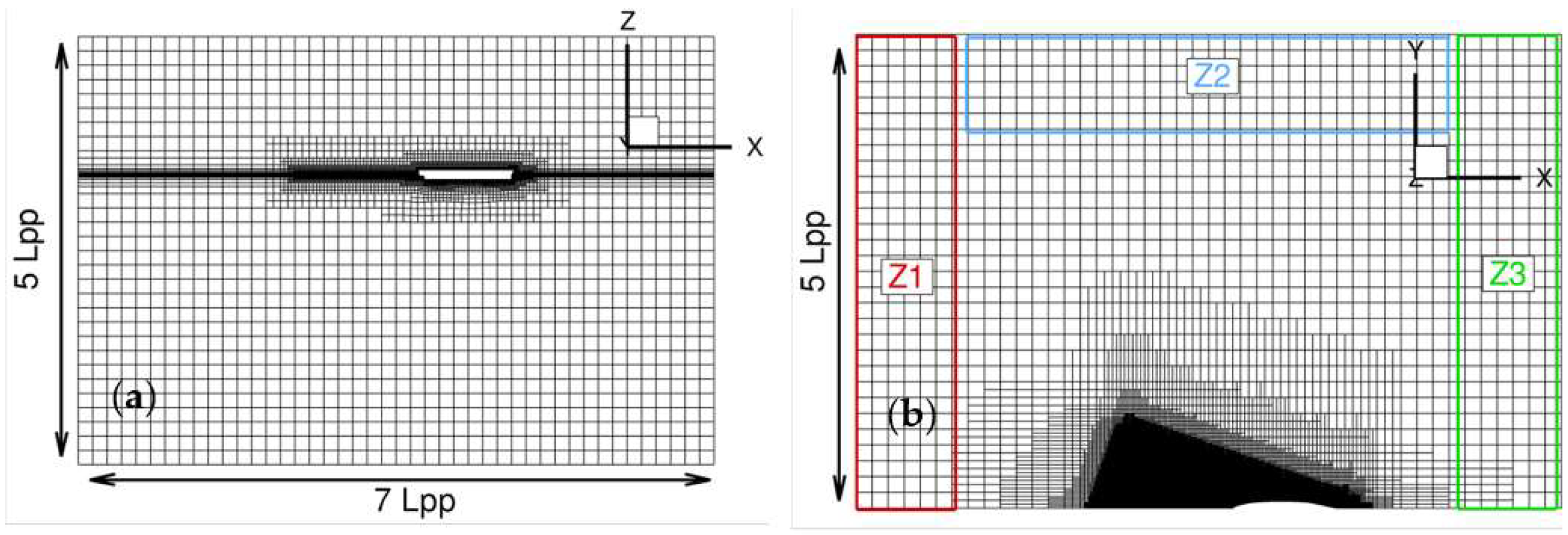
Article

Ship Bow Wings with Application to Trim and Resistance Control in Calm Water and in Waves

by
Dimitris Ntouras
,
George Papadakis
and
Kostas Belibassakis
*
School of Naval Architecture & Marine Engineering, National Technical University of Athens, 15780 Zografos, Greece
*
Author to whom correspondence should be addressed.
J. Mar. Sci. Eng. 2022, 10(4), 492; https://doi.org/10.3390/jmse10040492
Submission received: 7 March 2022 / Revised: 23 March 2022 / Accepted: 24 March 2022 / Published: 2 April 2022
(This article belongs to the Special Issue Energy Saving Devices for Ships)

Abstract

:
Flapping foils for augmenting thrust production have drawn attention as a means of assisting ship propulsion in waves due to their high efficiency rate compared to traditional screw propellers. However, they can also offer substantial resistance reduction when used as stabilizers. In this work, the aim is to investigate the feasibility of a symbiotic concept combining the ship’s propeller with a foil arranged at the ship’s bow at a fixed position operating as a trim-pitch stabilizer. The work presents results obtained from experiments conducted in the towing tank of the Laboratory of Ship and Marine Hydrodynamics of the National Technical University of Athens (LMSH NTUA), as well as results from an in-house CFD solver. The test cases focused on the resistance and the dynamic behavior of the wing–vessel configuration in calm water conditions and in head waves. All results were compared against the performance of a bare hull (without foil). The findings of this work are based both on numerical and experimental data and indicate that a bow wing in static mode can be used for trim-control of a vessel by altering the angle of attack leading to a possible drop in wave resistance both in calm water and in waves. In the latter case, utilizing the wing in head waves results in a significant reduction in the pitching and heaving responses of the vessel, which may lead to substantial enhancement of the propulsion performance.

1. Introduction

Maritime transportation is one of the main industries that supports global trade. Ship propulsion has been facilitated since the 20th century by the use of screw propellers driven by internal combustion engines. Global warming and the greenhouse effect have pushed research in the past few decades to investigate alternative means of propulsion. Humans have always been inspired by nature. Biomimetics is a research field that tries to imitate the mechanisms that have been selected by animals through the natural process of evolution. In aquatic environments, fish have adopted an unsteady motion of their bodies to propel themselves by efficiently extracting energy from sea currents and waves [1]. In the last decades, several studies have been done towards the emulation of this motion to augment ship propulsion, or even for use as a standalone system [2]. A series of experimental [3,4] and theoretical [5,6] approximations have been conducted to examine the exploitation of marine energy by using actively pitch-controlled foils. More recently, as part of Seatech H2020’s project entitled “Next generation short-sea ship dual-fuel engine and propulsion retrofit technologies” (https://seatech2020.eu/, accessed on 15 March 2022), a flapping wing with self-pitching control was considered along with the ship-hull form of a passenger car ferry vessel, and its performance in waves was quantified using experimental and numerical predictions in the Laboratory of Ship and Marine Hydrodynamics of NTUA [7]. In this work [7], the authors studied the ship’s flapping-wing system’s dynamic performance to illustrate the beneficial properties of such an arrangement. The results indicated that thrust augmentation due to the operation of the dynamic wing with controllable self-pitching motion in waves, as well as the decrease of added wave resistance due to ship stabilization, allowed the engine to operate in part-load at the same vessel ship speed.
In this work we extend previous research focusing on the effects of wings in static mode, but with a pre-defined inclination for studying its effects on ship trim-pitch control in calm water and in waves, as well as on ship resistance, using both computational tools and experimental data. Although the bow wing is considered static with respect to the ship, an important part of our study concerns the case when a ship oscillates in waves and, thus, the wing also operates in dynamic mode due to ship heave and pitch responses. Furthermore, the present work complements [7] with viscous calculations in the presence of the free surface. To this end, a series of simulations and experiments were conducted aiming to analyze the performance of a static wing in calm water conditions and in head waves. The paper is structured as follows: Section 2 sets the theoretical foundations of fluid-structure interaction (FSI) problems and implementation using a MaPFlow in-house CFD solver. Section 3 presents the numerical setup used for the CFD calculations, as well as a discussion about the chosen spatial and temporal discretization. In Section 4, the performance of the static wing is examined in a series of test cases. The results are divided into four different categories. Initially, an assessment of a bare hull is presented, which serves also as a validation and verification case of the numerical solver. Second, the effects of the configuration of the wing (including its supporting structure) on vessel resistance are examined. Moreover, Section 4.3, a study on the impact of foil pitch angle on ship resistance, is presented, and the performance of the configuration in regular waves is examined and compared with corresponding characteristics of a bare hull. Lastly, in Section 5, the basic outcomes of this investigation are described.

2. Numerical Methodology

In this section, a description of the numerical tool utilized in this work will be presented. The current analysis used CFD software MaPFlow [8]; a detailed analysis of the incompressible solver of the toolbox can be found in [9,10].

Solver Desription

MaPFlow solves unsteady Reynolds-averaged Navier–Stokes (URANS) equations in arbitrarily polyhedral grids using the finite volume method. The MaPFlow toolbox can handle both compressible and purely incompressible flows. In this work, the incompressible solver was used, coupled with a Volume of Fluid [11] method (VoF) to account for the presence of the free surface. The coupling of a divergent-free velocity field with pressure was performed using an artificial compressibility (AC) method. The method assumes a pseudo-relation between density and pressure during convergence. Once convergence is accomplished, the unknown variable fields satisfy the original set of incompressible equations. The unsteady flow fields were handled by employing a dual time-stepping technique. In this context, at each unsteady iteration, a variation of the unknown variables is assumed. Convergence is accomplished once this variation tends to zero. The unknown variables were pressure ( p ), 3-dimensional velocity (u), and an indicator function ( a ). The governing equations integrated over control volume Ω with a boundary of Ω are obtained by the following expression:
Γ Ω Q τ d Ω + Γ e Ω Q t d Ω + Ω ( F c F v ) d S = Ω S q d Ω
In the above equation, the vector Q = [ p , u , a ] T expresses the primitive variables; F c and F v denote the viscous and the inviscid fluxes, respectively; and the vector S q includes body forces (such as the gravitational field) and various source terms. Moreover, τ represents the pseudo-time variable, while t is the actual time.
The system is casted in primitive form. However, in order to advance the solution in time, the conservative variables U = [ 0 , ρ u , a ] T are used. To this end, the unsteady term is multiplied by the transformation matrix Γ e . In order to alleviate the poorly conditioned system arising in two phase flows with large density ratios, the Kunz preconditioner [12] Γ is used. The matrix Γ rescales the pseudo-time derivatives and ensures that the flux-difference scheme of Roe remains stable [13]. The matrices Γ e , Γ are given by:
Γ = [ 1 β ρ m 0 0 0 ρ m I u Δ ρ a l β ρ m 0 1 ] , Γ e = [ 0 0 0 0 ρ m I u Δ ρ 0 0 1 ]
where Δ ρ is the density difference between water density ( ρ w ) and the density of the air ( ρ a ). The density of the mixture ( ρ m ) is computed by the VoF function ρ m = α Δ ρ + ρ α , I is the 3-by-3 identity matrix, and β is the AC parameter that regulates the coupling between pressure and velocity.
Furthermore, in order to simulate numerical wave tanks, a technique for generating free surface waves should be integrated in the solver. MaPFlow generates free surface waves by employing implicit forcing zones near the boundaries of the domain [9,14,15]. In these regions, source terms are introduced into the momentum equation and drive the velocity field to the desired one. For wave generation, the desired velocity field is described by an analytical solution. An exponential function is used to decay the source terms away from the boundary exponentially. In addition, a common practice to ensure that no reflections occur in the outflow boundary of a numerical wave tank is to introduce damping zones. Their implementation is similar to the generation zones, although damping zones drive the vertical and transverse velocity components to zero.
For the spatial discretization process, which occurred within a cell-centered framework, evaluation of the two flux vectors at the face of each cell was required. The inviscid fluxes were computed using the approximate Riemann solver of Roe. The viscous fluxes were computed by a central finite difference scheme equipped with a directional derivative to account for the skewness of the mesh. Due to the particular nature of each unknown field, a different reconstruction scheme was adopted for each one of them. For the velocity field, an unlimited piecewise linear interpolation (PLR) scheme was used. For the pressure field, a PLR scheme was used away from the interface. However, in the case of strong gradients of VoF, a density-weighted interpolation scheme was used to account for discontinuity of the gradient due to hydrostatic pressure. Finally, the VoF field was reconstructed using a high-order compressive interpolation scheme.
The temporal discretization scheme was handled implicitly by considering a series of successive-level backwards times [16]. For the pseudo-time derivatives, a first-order Euler scheme was used, while the local time-stepping technique was utilized to facilitate convergence. Fluid–structure interaction (FSI) problems, such the ones discussed in the present article, were handled in MaPFlow by communicating the loads on the solid boundary to a rigid body dynamic solver, which in turn computed new displacements by solving a mass–spring–damper model. The dynamic equations were linearized using the Newmark-β method. Internal iterations were performed at each timestep between the fluid solver and dynamic solver until convergence of displacements. This process led to a strong coupling between the two.
The following sections present simulations of a rigid body with two degrees of freedom: the pitch and heave motions. The displacement of the body was absorbed by the mesh nodes by performing a deformation algorithm. This work adopted a distance-based damping technique that was introduced in [17].

3. Numerical Setup

For the numerical simulations, a single wave tank was used. Its basic dimensions are illustrated in Figure 1. In order to save computational resources, only a half-model was simulated by applying symmetry conditions. In Figure 1, the implicit source zones applied near the boundaries of the domain are also depicted. In the case of calm water conditions, all zones served as damping zones aiming to reduce the amplitude of the vertical velocity component. In this case, all boundary conditions were set to far-field. However, in the case of head waves, Z3 was used for generating waves, Z2 for damping the transverse velocity component, and Z3 damped the vertical component of velocity, as before. The boundary conditions were the same as in the first case with the exception of the lateral boundary, which was set to symmetry. Moreover, it is noteworthy that, in order to avoid strong transient effects on the body, the model was accelerated using a hyperbolic tangent function for 1000 timesteps in all case studies, which was found to provide better numerical convergence characteristics.
The body plan of the ferry ship hull model with a length of L = 3.3 m that was considered is shown in Figure 2, and basic data concerning the ship hull considered in this study can be found in Section 2.2 of Ref. [7]. Prior to the systematic runs, a grid independence study for a bare hull in calm water conditions was conducted, and the results are presented in Table 1 and Figure 3. The study regarded the nominal speed ( V n o m = 1.42 m/s), which corresponds to Fn = 0.25, for the heavier condition (T = 0.135 m) in calm water conditions. The nominal ship speed was selected on the basis of information and data concerning the operational speed for ferry ships similar to the one considered here. The vessel was able to rotate around the transverse y-axis (pitch) and move vertically (heave). Three different grids were generated, consisting of 902 thousand (G1), 2.46 million (G2), and 6.11 million (G3) cells. The parameters used for grid refinement were the number of cells on the body (surface mesh), the number of the cells at the height of the generated waves, and the number of cells per wavelength. The same timestep was adopted for all simulations, and it was small enough keep the mean CFL value below 1 in the finest mesh (approximately 0.60). In Table 1, the results of the independency study are shown. Convergence of the results was noted between the G2 and G3 grids, since the difference was less than 1% for resistance and sinkage and 3.5% for the trim angle. Thus, the G2 grid was chosen for the simulations.
Furthermore, in order to choose the right timestep for the computations, a similar study was conducted. The three different timesteps were chosen based on T r e f = L s / V n o m , where L s is the ship length, and V n o m is the nominal advance speed ( V n o m = 1.42   m / s ). The results can be found in the following table, as well. Since the problem converged in a steady solution, all cases produced the same results. For the rest of simulations, the intermediate time-step was chosen.
In order to provide a better illustration of the convergence studies, in Figure 3, the results of the grid and time-step independency study are shown in terms of vessel resistance.
Furthermore, in order to estimate the spatial discretization error, the Grid Convergence Index (CGI) was calculated based on the Richardson extrapolation [18], Firstly, a representative cell size was defined as h for each mesh. If N is the total number of cells in each grid and V i is the volume of the cell i , then
h = [ 1 N i = 1 N V i ] 1 3
Moreover, let index 1 represent the finest discretization with a representative cell size of h 1 , while 2 and 3 represent the medium and the coarse grids, respectively. Then, the ratios of the discretization can be defined as r i j = h i / h j . The apparent order p of the method was calculated based on:
where
p = 1 ln ( r 21 ) | ln | ε 32 / ε 21 | + q ( p ) |
q ( p ) = ln ( r 21 p s r 32 p s ) ,
s = s g n ( ε 32 / ε 21 ) ,
where ε i j = φ i φ j is the difference between the computed value φ i . From the above definitions, the following values can be computed:
(i)
the extrapolated value
φ e x t 21 = r 21 p φ 1 φ 2 r 21 p 1 ,
(ii)
the approximate relative error
e a 21 = | φ 2 φ 1 φ 1 | ,
(iii)
the extrapolated relative error
e e x t 21 = | φ e x t 21 φ 1 φ e x t 21 | ,
(iv)
the fine GCI
G C I f i n e 21 = 1.25   e e x t 21 φ 1 r 21 p 1 .
The corresponding values are reported in Table 2.
Figure 4 presents a flow visualization of the density field on the hull of a ship. An elevation of the free surface was noted close to the bow; however, in the rest of the hull, the free surface was almost level. The figure also includes a contour of the y + values on the hull. The first grid node was placed 0.01 mm away from the solid boundary, which led to y + < 1 almost everywhere on the hull. The no-slip boundary condition imposed on the model can lead to a singular behavior of the free surface on the wall. As the free surface deformed due to the model’s motion, the no-slip boundary condition did not allow convection of the volume fraction on the wall. This transient behavior can significantly affect the convergence of the simulation. In order to avoid this, the values of a were swept within a user-specified distance normal to the wall. As described in [19], this distance was taken as 3 · 10 4 for a body-unit length.

4. Results and Discussion

This section presents results for the vessel with and without the wing in calm water conditions and head waves. The numerical simulations were compared with available experimental data. The experiments were conducted in the towing tank of LSMH at NTUA (see also [7]). The results were divided in four subsections. First, the base hull was assessed for two different drafts with six Froude numbers between 0.043 and 0.28 and compared with the experimental data. The second subsection focuses on the effect of the wing and its supporting structure in calm water conditions. In addition, a quantification of the impacts of the experimental setup was assessed. The third paragraph presents a parametric study regarding the impact of the angle of attack in the resistance of the model in calm water conditions. To this end, nine different angles were considered between −5 and 3.6 degrees. Finally, the last paragraph assesses the effect of a static wind arranged at the bow in head waves, presenting both experimental and numerical results.
The experiments regarded the performance of the vessel with and without the operation of the dynamically controllable flapping thruster. The dimensions of the NTUA towing tank are: a length of 100 m, a breadth of 4.6 m, and a maximum depth of 3 m. The maximum speed of the carriage is 5 m/s. The model was constructed out of wood and prepared for testing at two selected drafts: Τ = 0.135 m and T = 0.125 m. The foil was constructed of polyvinyl chloride (PVC) that was polished and painted. The foil planform shape was orthogonal, and its span was s = 0.50 m with a span-to-chord ratio of s/c = 4; thus, its aspect ratio was AR = 4. Based on data from an extended collection of previous works and experience concerning the performance of flapping thrusters (see, e.g., [2]), an uncambered orthogonal wing of constant NACA0012 sections was also used in the present study. The wing was placed 0.150 m ahead of the front perpendicular and 0.075 m under the ship’s keel. This work focused only on the effect of a static wing in front of the ship’s bow.

4.1. Dynamic Trim and Sinkage of the Bare Hull

Considering only the hull, Figure 5 presents a comparison of the numerical predictions against the measurements for the two drafts. It is evident that the computational results were close to the experimental data, especially for the heavier condition (T = 0.135 m). For the lighter condition, larger deviations were evident. These may be attributed to the water level being exactly at the transom level for the lighter draft, introducing uncertainties both in the measurements and the simulations.
Moving on to the comparison of the trim and sinkage characteristics of the vessel, Figure 6a illustrates the predicted trim values against the measured ones for the two drafts. Although deviations were noted between the two approximations, the differences were considered minor since, in all cases, they remained less than 0.05 degrees. It was noted, however, that the oscillations of the trim data at the higher Froude numbers evident in the measurements were not reproduced by the numerical results. In Figure 6b, the comparison of the sinkage between the experiments and the simulations can be seen. The differences between the computational and the experimental data were more pronounced in the low Froude number regime up to V = 1 m/s. In this range, the simulations predicted larger displacements that the measurements. As the Froude number increased, the comparison became better. Summarizing the results, the two approximations produced similar results, although there were some major deviations for the lighter draft.

4.2. Effect of a Wing Arranged in Front of the Bow in Calm Water Conditions

Prior to examining the effects of a static wing on trim control and resistance of a vessel in both calm water conditions and head waves, it is important to discuss some differences between the numerical setup and the experimental configuration. To this end, a series of simulations were performed to quantify the effects of the wing and its supporting structure in the total resistance of the model. The wing was fixed with zero angle of attack (AoA). This quantification process will provide better insight into the results and the comparison between the numerical and experimental data.
The whole experimental setup (vessel–wing configuration) is presented in Figure 7. As noted on the picture, apart from the dynamic wing, the vane and the supporting skegs are present. The vane is used to measure the local AoA needed for the dynamic wing pitch controller, while the skegs support the dynamic wing. In order to obtain reliable readings of the time-dependent flow angle of attack, which are used in the control of the dynamic wing in waves (see Belibassakis et al. [7]), the dimension of the vane was selected as large with respect to the tank model size and had a significant effect on the total resistance of the system. The latter effect is expected to be completely eliminated in full-scale applications where the dimension of the vane will be negligible with respect to the ship. Moreover, the effect of the vertical struts is expected to be reduced by optimal design of the supporting system for restraining the foil in the water. Thus, in order to quantify the effect of each component, measurements and numerical simulations were employed, and, regarding the measurements, additional experiments were conducted excluding the vane.
In the CFD analysis, the vane was omitted, and the wing was considered fixed at zero inclination (AoA = 0°). The hull, the supporting skegs, and the wing were modelled. An overview of the mesh used is presented in Figure 8. The computational mesh for the hull was the same as that in the previous section, while on the skegs and the wing, a surface of 15,000 cells was generated. Additionally, in the free surface region, the mesh was refined near the skeg to capture the skeg-generated wave system, and refinement boxes were added around the configuration to resolve the effects of the wake.
The experimental results with and without the presence of the vane for both drafts are presented in Figure 9 and Figure 10. The CFD simulations were considered for three velocities, V = 1 m/s, 1.3 m/s, and 1.42 m/s, which correspond to the Froude numbers 0.176, 0.22, and 0.25, respectively. More specifically, the comparison for the heavy draft is presented in Figure 9, while the lighter draft is shown in Figure 10.
Firstly, from both figures, it is clear that the wing and the supporting structure configuration added extra resistance to the vessel that increased with the Froude number. Furthermore, it is shown that the vane accounted for approximately 15% of the total resistance. This was attributed to its large size, as previously discussed. However, in the case of a full-scale vessel, it is considered that the vane will remain the same (it does not scale with the rest of the geometry), and, consequently, in full scale, the vane-induced resistance should be negligible. The numerical predictions and the measurements, as shown in Figure 9 and Figure 10 for the two drafts, respectively, were in very good agreement without the vane. This reinforces the experimental observation that the presence of the vane resulted in a significant increase in the model’s resistance.
Furthermore, using the CFD solution, the contribution of each individual component (hull, skegs, and wing) was retrieved. The contribution of each component of the configuration in the total resistance can be found in the two following tables (Table 3 and Table 4) for the two drafts.
It is evident that the resistance of the skegs and the foil significantly increased the resistance of the model. The resistance of the supporting skegs was about 9.5% of the total value, while the wing at an inclination of AoA = 0° constituted around 12% of the total resistance.

4.3. Effect of the Foil Inclination in Calm Water Conditions

In order to investigate the utilization of the wing, trimming experimental and computational studies were performed. Measurements were conducted with the wing positioned at four different angles: AoA = −3.1°, −1.6°, 0°, and 1.6°, where the negative sign indicated a nose-up foil inclination. The experiment was conducted considering the full configuration (skegs, wing, and vane) at the nominal Fn = 0.25 (V = 1.42 m/s) for the heavy condition (T = 0.135 m). The results are presented in Table 5 for the resistance, trim angle and sinkage.
It is evident that, with respect to resistance when the wing is positioned at zero inclination (AoA = 0°), a change in the angle had a beneficial effect. Indeed, for all the angles presented above, there was a drop in the measured resistance, attributed to different dynamic trim and sinkage.
Contrary to the experimental setup, the CFD simulations were performed without the supporting skegs and vane. The mesh considered in the previous simulations was employed (wing at AoA = 0°), and using a mesh deformation algorithm, the angle of attack of the wing was adjusted. The measurements included the whole configuration. In order to compare them with the CFD predictions, the effect of the vane and the skegs was subtracted from the measured data. Regarding the vane, this was accomplished by using the experimental measurements with and without the vane (see Figure 9). To quantify the effect of the skegs on resistance, the CFD predictions of the hull, skegs, and wing system were exploited (see Table 3). The skegs’ resistance was normalized as a percentage of the total resistance. By assuming that it remained constant for the various configurations, the experimental data were corrected, enabling the direct comparison of the measurements and the numerical CFD predictions, as presented in Figure 11. In the same figure, the resistance of the hull with the wing and the skegs for the same Froude number (Fn = 0.25) is indicated by a thick dashed line.
The CFD simulations were conducted for the additional wing angles of −0.8°, −1.2°, −2°, −2.6°, and −5°. It is clear from Figure 11 that the reduction in resistance for an AoA ranging from −2° to −0.8° was also predicted by the numerical simulations. When the wing was positioned below −2°, the resistance increased. Compared to the measurements, the simulations predicted a smaller benefit in the total resistance; however, they followed the experimental trend, at least for the negative angles. Larger deviation between the measurements and the simulations was noted when the wing was placed at AoA = 1.6° (positive implies a nose-down foil inclination).
Finally, the predicted and measured dynamic trim and sinkage values for the various AoAs are presented in Figure 12 and Figure 13, respectively. As concerns the experimental data in these figures, the original values were plotted (including the supporting skegs and vane), since it was not feasible to decouple the contribution of each component from the dynamic behavior of the model. Despite a different setup, the comparison between the two approximations was fairly good for a wide range of AoA. At 0° and 1.6°, the predicted sinkage and trim almost coincided. Even though, for negative AoAs, the deviation between the CFD and the experiments increased, they were still within acceptable limits, with the largest differences being 0.05° for trim and 0.05 cm for sinkage.

4.4. Effect of the Wing in the Presence of Regular Waves

In this section, the effects of the static wing on the model were investigated under the excitation of regular waves. Simulations with and without the foil were performed for four different head-incident regular waves. Numerical predictions were compared with experiments that were conducted at the NTUA towing tank for the bare hull and static wing configurations. The frequencies of the incident waves were f = 0.55 Hz, 0.65 Hz, 0.67 Hz, and 0.75 Hz. The corresponding ratios of wavelength to ship length ( L w / L s ) were 1.66, 1.12, 1.20, and 0.87. In all cases, the wave height was 0.06 m. It is noted here that the dynamic responses of the ship and wing system were considered in an extended band of frequencies around the resonance in order to obtain useful results for the behavior in irregular waves characterized by a spectrum.
As a first step, a time-step sensitivity study was conducted for the main frequency (f = 0.67 Hz). Three time-steps were considered, and the results are summarized in Table 6. Convergence was noted for the two finest time-step discretizations. The smallest time-step was chosen for all simulations to ensure consistency of the results in larger wave frequencies, as well.
For better understanding of the wing’s influence under the excitation of different waves, in Figure 14, Figure 15 and Figure 16, the signals of resistance, ship trim, and sinkage are plotted in one encounter period. All signals suggested better performance characteristics when a static foil was arranged in front of the bow.
By examining the signal of resistance in the case of the bare hull configuration, a sudden increase in the loads at approximately 0.4 of the encounter frequency was noted for the two larger wave frequencies (Figure 15 and Figure 16). At that instance, the pitch of the model was at its maximum value (the positive pitch sign indicates bow down). The sudden increase was attributed to the slamming of the ship’s bow at a wave crest. In the case of the augmented configuration, a delay in the signal of pitch was noted. This phase shift prevented the slamming of the bow, leading to a smoother resistance signal.
Moreover, regarding the effect of the static wing on vessel resistance, it is evident that in all studied cases the foil had a positive effect. In the above figures, the mean resistance over an encounter cycle is denoted by dashed line. It is evident that the foil critically reduced the heave and pitch responses. This had a direct impact on resistance, showing a reduction of up to 34% when the foil was present (in static conditions). The reductions in resistance for all the wavelengths considered are summarized in Table 7.
The effect of the wing can be further illustrated by the response amplitude operators, which are presented in Figure 17, a comparison between numerical and experimental results for regular waves with and without foil. The figure presents the response amplitude operators for (a) nondimensional heave and (b) pitch, where A is the wave amplitude and k is the wave number for the two degrees of freedom: pitch (ξ5) and heave (ξ3). The heave was nondimensionalized based on the wave amplitude (A), while pitch used wave number (k) times wave amplitude (A). The figure includes both experimental and computational results. First, it was noted that the agreement between the computational results and the measurements was fair. Larger deviation was seen in the heave amplitude for the shortest wavelength in the case of the bare hull. Aside from that, the CFD calculations were in accordance with the experimental results for the bare hull. Regarding the comparison for when the foil was present, it was noted that, although the CFD results followed the experimental trends, there was almost-constant deviation from the measurements. Since in the simulations only the foil was considered, this deviation was attributed to the different configurations considered in the experiment and the simulations.
From both the numerical simulations and the measurements, the same qualitive conclusions can be drawn. The wing significantly reduced the amplitude of the pitch motion. The heave was reduced only for the smaller wavelengths, while in larger wavelengths the differences were smaller.
As a last remark, two comparisons between the flow–field with and without the foil are presented in Figure 18 and Figure 19. The first figure illustrates an iso-surface of the density field for ρ m = 500   kg / m 3 colored by the vertical coordinate in the case of the heavier draft with an incident wave frequency of 0.67 Hz. The two snapshots are in the case of the maximum negative pitch amplitude. From the flow visualizations, it can be seen that smaller amplitude of pitch motion occurred when foil was deployed at the ship’s bow. The second figure regards the comparison of the pressure field at the instance of the slamming of the bare hull on the free surface, which occurred at t/T = 0.45 (see Figure 15a). From the comparison, it is clear that large pressure values occurred at the ship’s bow, while smaller values of pressure were noted in the case of the augmented configuration. Moreover, examining the pressure field around the foil, an upward force was created that prevented the hull from slamming on the free surface.

5. Conclusions

In this work the effects of a static foil placed at the bow of a ship hull with a predefined inclination angle were investigated in both calm water conditions and head waves. Several parametric studies were conducted for a ferry ship hull model with a length of 3.3 m at Froude number 0.25 with a bow wing of orthogonal planform and NACA0012 sections in order to better illustrate the effects of flow conditions and configuration set-up on the model’s resistance. In the examined cases, the system had two degrees of freedom: the pitch and heave motions. The numerical results obtained by CFD analysis based on in-house codes were presented and compared with experimental data measured using a small-scale model in a towing tank and were found to be in good agreement. More specifically, the resistance of the foil and the supporting system was quantified in calm water conditions. It was shown that the wing can be used for ship trim control with the possibility to obtain a reduction in the total resistance of the system of the order of 5% if the effects of skegs supporting the foil in the water in front of the ship bow were minimized, which could be achieved to some extent by engineering design. Furthermore, the performance of the system in monochromatic head incident waves was examined. In this case, both numerical and experimental results showed an improved performance of the system due to a significant decrease in added resistance in the waves of the studied configuration of the order of 12–34% compared to the bare hull, with the larger values achieved near the resonance conditions. Future work will be focused on the exploitation of the present method and results for the optimal design of the studied system.

Author Contributions

This work was supervised by G.P. and K.B. The RANSE numerical scheme was developed by D.N. and G.P. The draft of the text was prepared by all the authors, and the numerical simulations were handled by D.N. and G.P. All authors have read and agreed to the published version of the manuscript.

Funding

The present work was supported by the Seatech H2020 project funded by the European Union’s Horizon 2020 research and innovation program under the grant agreement No 857840.

Institutional Review Board Statement

Not applicable.

Informed Consent Statement

Not applicable.

Data Availability Statement

Not applicable.

Acknowledgments

The present work was supported by the Seatech H2020 project and received funding from the European Union’s Horizon 2020 research and innovation program under grant agreement No. 857840. The opinions expressed in this document reflect only the authors’ views and in no way reflect the European Commission’s opinions. The European Commission is not responsible for any use that may be made of the information contained here.

Conflicts of Interest

The authors declare no conflict of interest.

Nomenclature

Fn Ship Froude Number
VShip Advance Speed
V n o m Ship Nominal Advance Speed (1.42 m/s)
TShip Draft
LsShip Length
s, cWing Span and chord length
LwWave Length
fWave Frequency
kWave Number
AWave Amplitude
R p Mean Resistance
ξ3, ξ5Heave, Pitch
A φ Amplitude of Parameter φ
φ ¯ Mean Value of Parameter φ

References

  1. Triantafyllou, M.S.; Triantafyllou, G.S.; Yue, D.K.P. Hydrodynamics of Fishlike Swimming. Annu. Rev. Fluid Mech. 2000, 32, 33–53. [Google Scholar] [CrossRef]
  2. Wu, X.; Zhang, X.; Tian, X.; Li, X.; Lu, W. A review on fluid dynamics of flapping foils. Ocean Eng. 2020, 195, 106712. [Google Scholar] [CrossRef]
  3. Bøckmann, E.; Steen, S. Model test and simulation of a ship with wavefoils. Appl. Ocean Res. 2016, 57, 8–18. [Google Scholar] [CrossRef]
  4. Bøckmann, E.; Steen, S. Experiments with actively pitch-controlled and spring-loaded oscillating foils. Appl. Ocean Res. 2014, 48, 227–235. [Google Scholar] [CrossRef]
  5. Filippas, E.S.; Papadakis, G.P.; Belibassakis, K.A. Free-surface effects on the performance of flapping-foil thruster for augmenting ship propulsion in waves. J. Mar. Sci. Eng. 2020, 8, 357. [Google Scholar] [CrossRef]
  6. Belibassakis, K.A.; Politis, G.K. Hydrodynamic performance of flapping wings for augmenting ship propulsion in waves. Ocean Eng. 2013, 72, 227–240. [Google Scholar] [CrossRef]
  7. Belibassakis, K.; Filippas, E.; Papadakis, G. Numerical and Experimental Investigation of the Performance of Dynamic Wing for Augmenting Ship Propulsion in Head and Quartering Seas. J. Mar. Sci. Eng. 2021, 10, 24. [Google Scholar] [CrossRef]
  8. Papadakis, G. Development of a Hybrid Compressible Vortex Particle Method and Application to External Problems including Helicopter Flows. Ph.D. Thesis, National Technical University of Athens, Athens, Greece, 2014. [Google Scholar]
  9. Ntouras, D.; Papadakis, G. A Coupled Artificial Compressibility Method for Free Surface Flows. J. Mar. Sci. Eng. 2020, 8, 590. [Google Scholar] [CrossRef]
  10. Mavrakos, A.S.; Konispoliatis, D.N.; Ntouras, D.G.; Papadakis, G.P.; Mavrakos, S.A. Hydrodynamics of Moonpool-type Floaters: A theoretical and a CFD formulation. Energy 2021, 15, 570. [Google Scholar] [CrossRef]
  11. Hirt, C.W.; Nichols, B.D. Volume of Fluid (VOF) Method for the Dynamics of Free Boundaries. J. Comput. Phys. 1981, 39, 201–225. [Google Scholar] [CrossRef]
  12. Kunz, R.F.; Boger, D.A.; Stinebring, D.R.; Chyczewski, T.S.; Lindau, J.W.; Gibeling, H.J.; Venkateswaran, S.; Govindan, T.R. A preconditioned Navier-Stokes method for two-phase flows with application to cavitation prediction. Comput. Fluids 2000, 29, 849–875. [Google Scholar] [CrossRef]
  13. Venkateswaran, S.; Lindau, J.; Kunz, R.; Merkle, C. Preconditioning algorithms for the computation of multi-phase mixture flows. In Proceedings of the 39th Aerospace Sciences Meeting and Exhibit, Reno, NV, USA, 8–11 January 2001. [Google Scholar] [CrossRef] [Green Version]
  14. Ntouras, D.; Manolas, D.; Papadakis, G.; Riziotis, V. Exploiting the limit of BEM solvers in moonpool type floaters. J. Phys. Conf. Ser. 2020, 1618, 052059. [Google Scholar] [CrossRef]
  15. Perić, R.; Vukčević, V.; Abdel-Maksoud, M.; Jasak, H. Optimizing wave-generation and wave-damping in 3D-flow simulations with implicit relaxation-zones. Coast. Eng. 2021, 171, 104035. [Google Scholar] [CrossRef]
  16. Biedron, R.; Vatsa, V.; Atkins, H. Simulation of Unsteady Flows Using an Unstructured Navier-Stokes Solver on Moving and Stationary Grids. In Proceedings of the 23rd AIAA Applied Aerodynamics Conference, Toronto, ON, Canada, 6–9 June 2005; pp. 1–17. [Google Scholar] [CrossRef] [Green Version]
  17. Zhao, Y.; Tai, J.; Ahmed, F. Simulation of micro flows with moving boundaries using high-order upwind FV method on unstructured grids. Comput. Mech. 2001, 28, 66–75. [Google Scholar] [CrossRef]
  18. Celik, I.B.; Ghia, U.; Roache, P.J.; Freitas, C.J.; Coleman, H.; Raad, P.E. Procedure for Estimation and Reporting of Uncertainty Due to Discretization in CFD Applications. J. Fluids Eng. 2008, 130, 078001. [Google Scholar] [CrossRef] [Green Version]
  19. Nichols, D.S. Development of a Free Surface Method Utilizing an Incompressible Multi-Phase Algorithm to Study the Flow about Surface Ships and Underwater Vehicles. Ph.D. Thesis, Mississippi State University, Starkville, MS, USA, 2002. [Google Scholar]
Figure 1. Overview of the computational domain. (a) Side view and (b) top view of the grid. The forcing zones (Z1, Z2, Z3) are noted on the right figure.
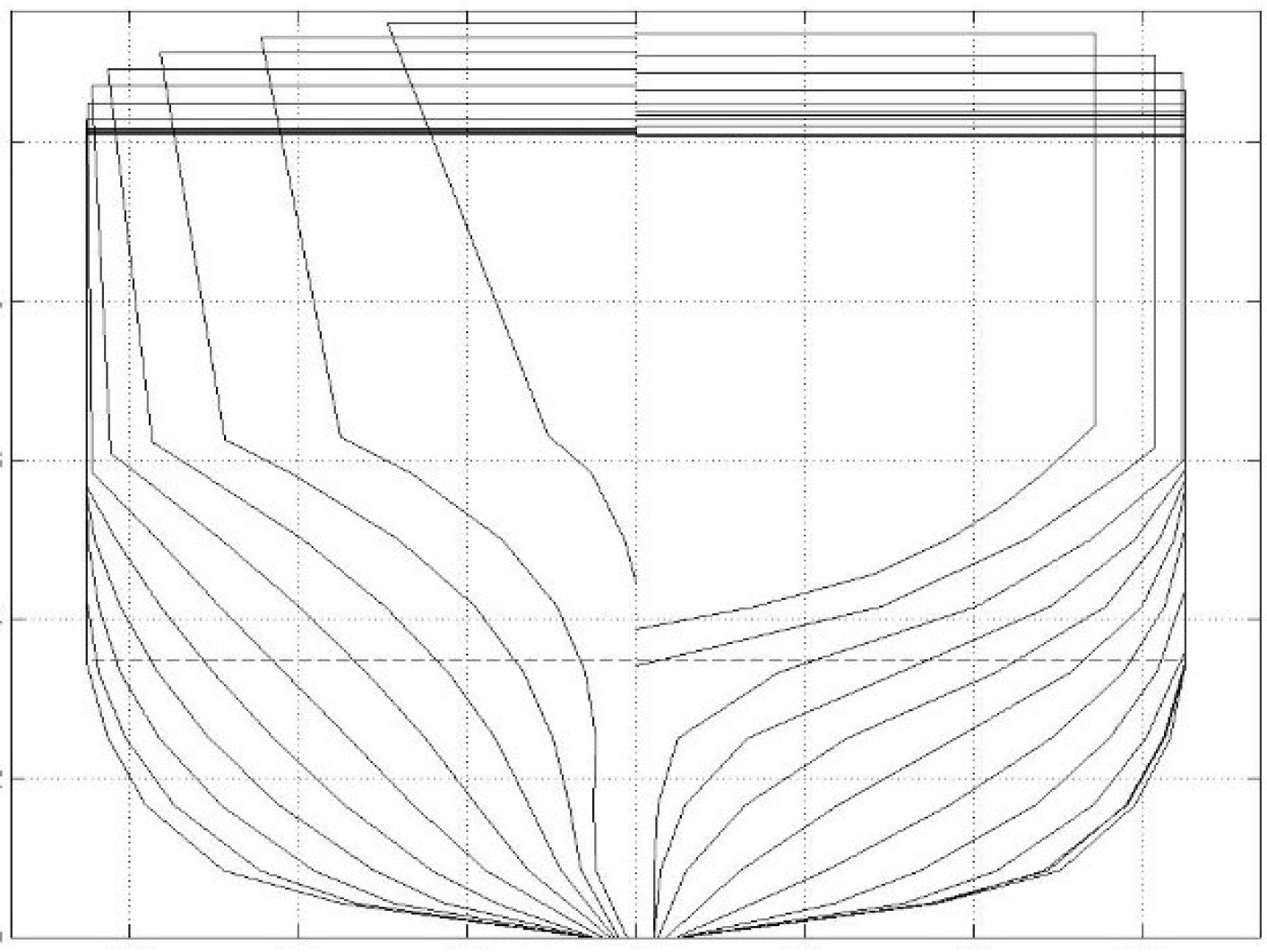
Jmse 10 00492 g001
Figure 2. Body Plan of the ferry ship hull.
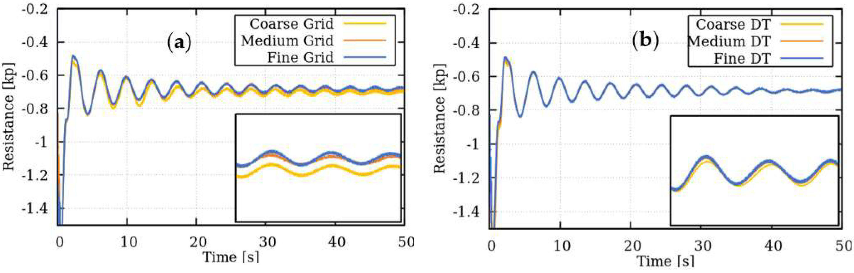
Jmse 10 00492 g002
Figure 3. (a) Grid density and (b) time-step independency study.
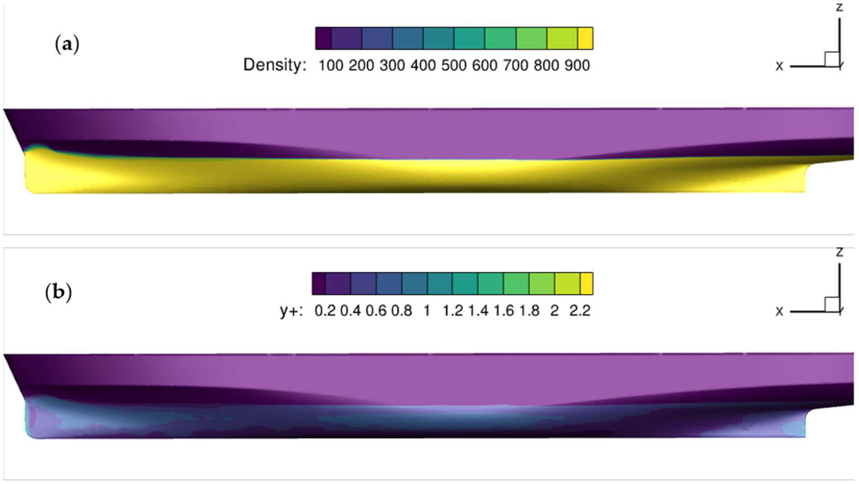
Jmse 10 00492 g003
Figure 4. (a) Free surface elevation and (b) y+ values on the ship hull in calm water conditions for draft T = 0.135 m and Fn = 0.25.
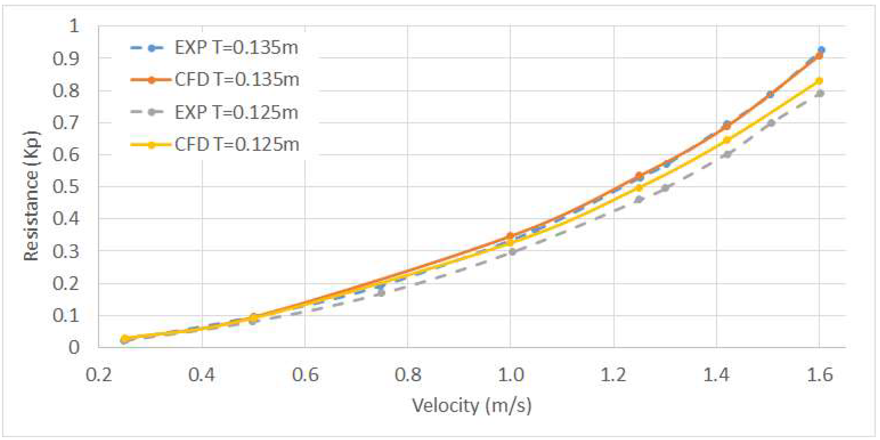
Jmse 10 00492 g004
Figure 5. Comparison of the CFD data and experimental predicted resistance for the two drafts.
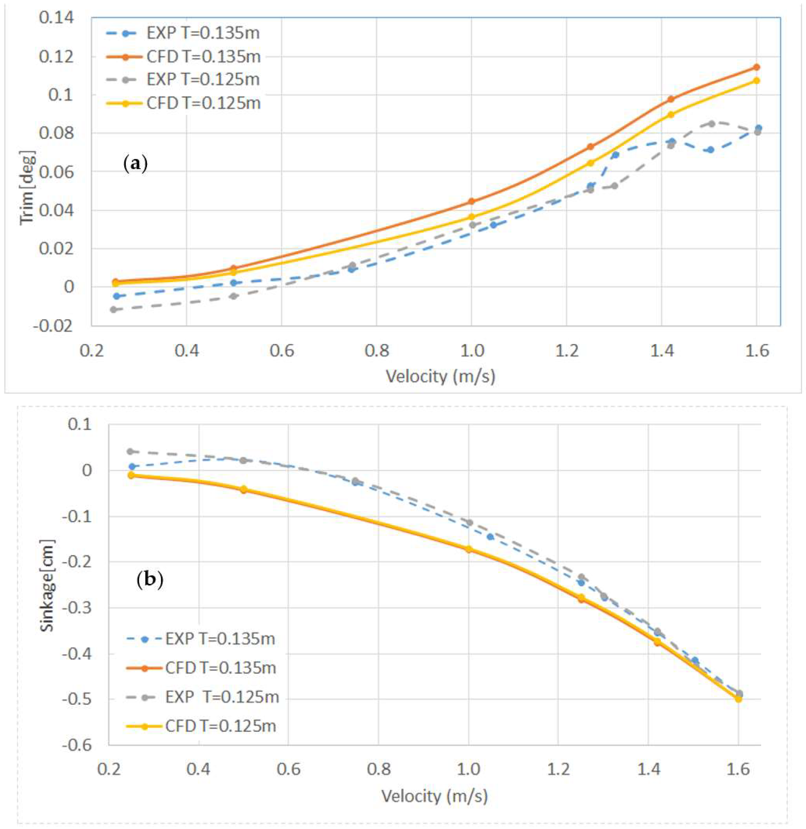
Jmse 10 00492 g005
Figure 6. Comparison of the CFD data and experimental predictions for the two drafts for (a) trim angle and (b) sinkage.
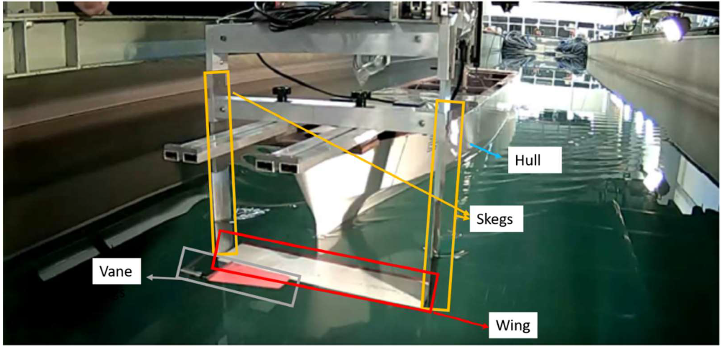
Jmse 10 00492 g006
Figure 7. Experimental configuration of the dynamic wing arranged at the bow of the ferry ship model tested in the tank of LMSH at NTUA.
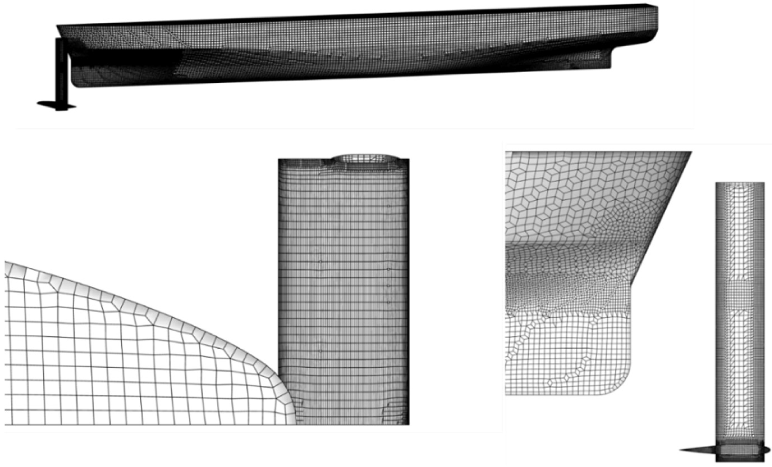
Jmse 10 00492 g007
Figure 8. Computation mesh of the hull with the skegs–wing configuration.
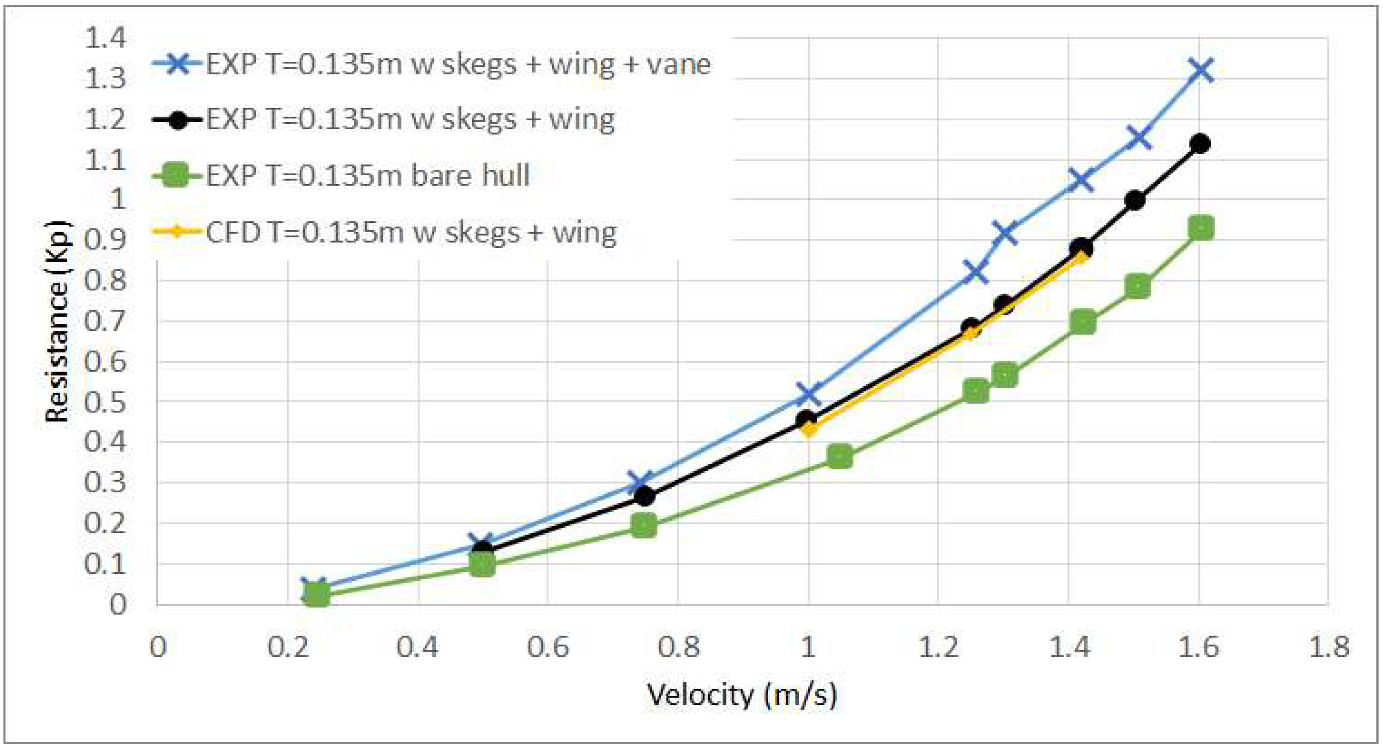
Jmse 10 00492 g008
Figure 9. Comparison of the various configurations for heave draft T = 0.135 m.
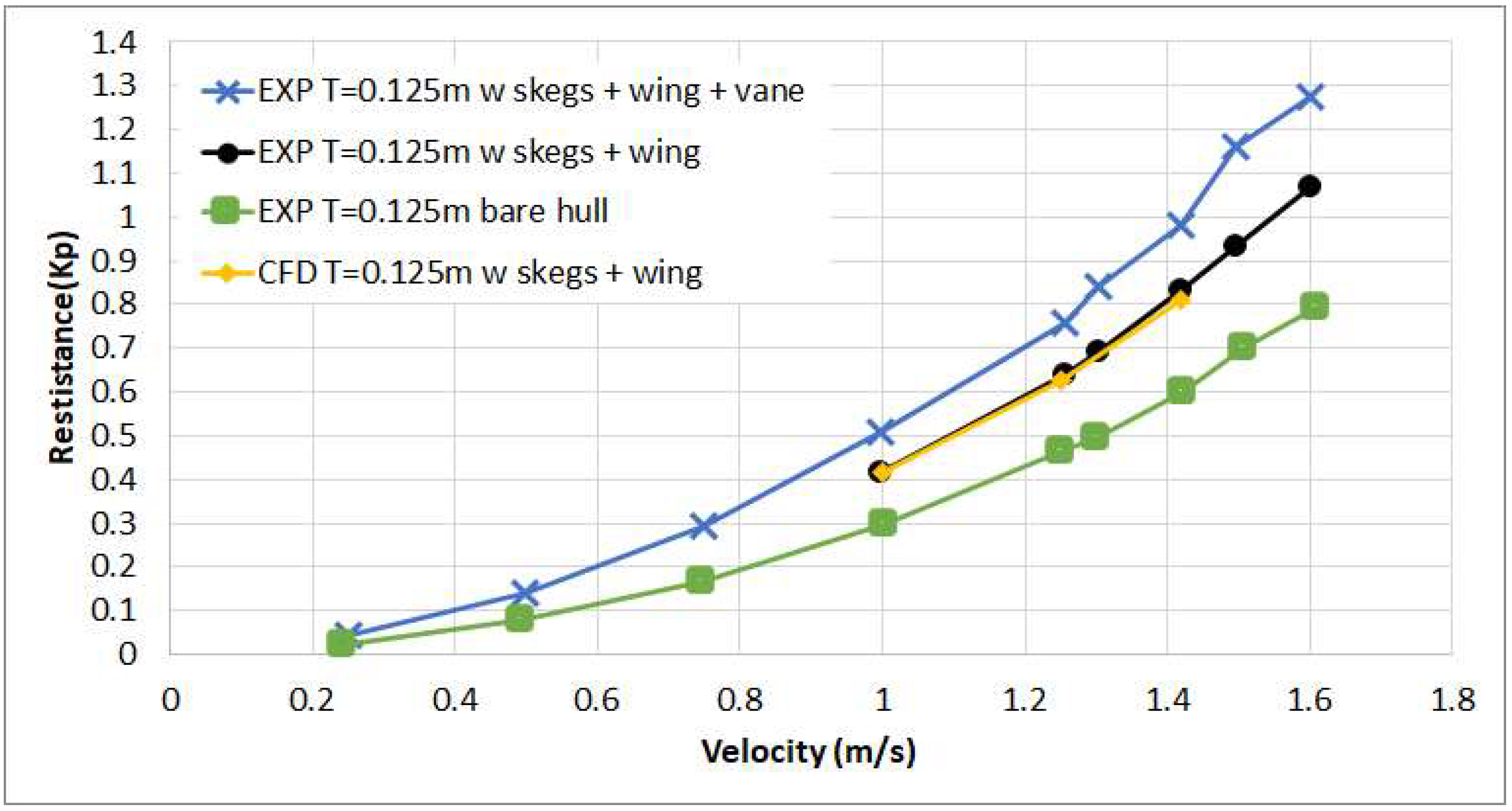
Jmse 10 00492 g009
Figure 10. Comparison of the various configurations for heave draft T = 0.125 m.
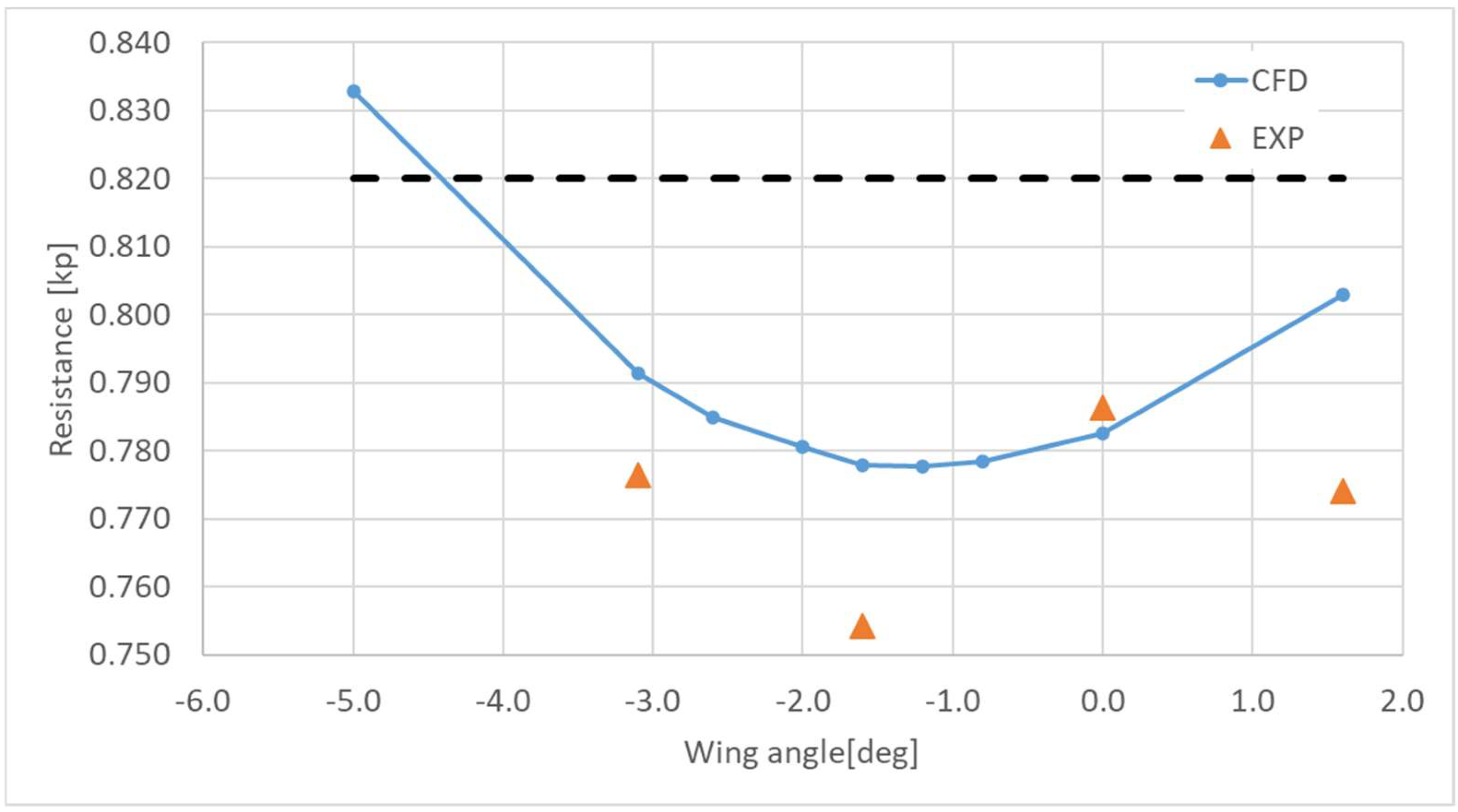
Jmse 10 00492 g010
Figure 11. Comparison of the predicted resistance for the various angles of attack. The results concern the nominal speed (V = 1.42 m/s) for the heavier condition (T = 0.135 m). The experimental data were corrected by subtracting the resistance of the skegs and vane.
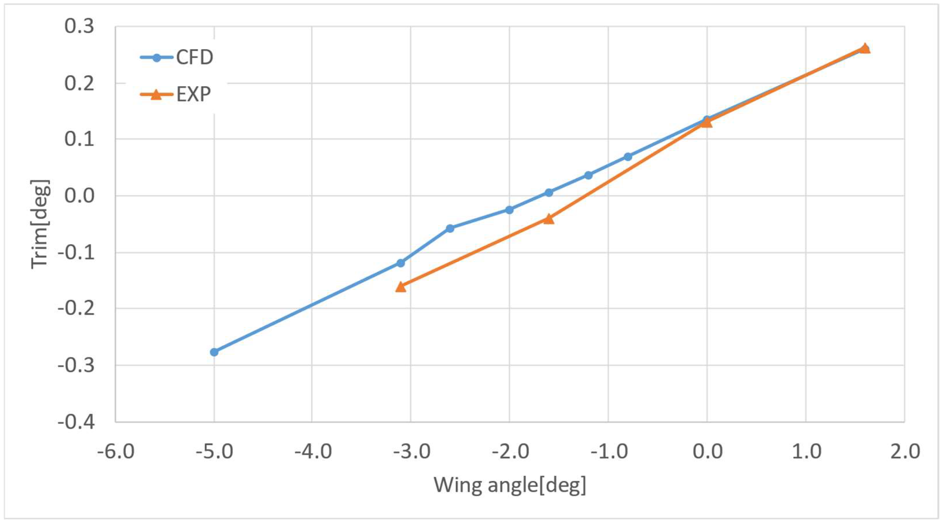
Jmse 10 00492 g011
Figure 12. Comparison of the predicted trim angle for the various angles of attack. The results concern the nominal speed (Vnom = 1.42 m/s) for the heavier condition (T = 0.135 m).
Jmse 10 00492 g012
Figure 13. Comparison of the predicted sinkage for the various angles of attack. The results concern the nominal speed (Vnom = 1.42 m/s) for the heavier condition (T = 0.125 m).
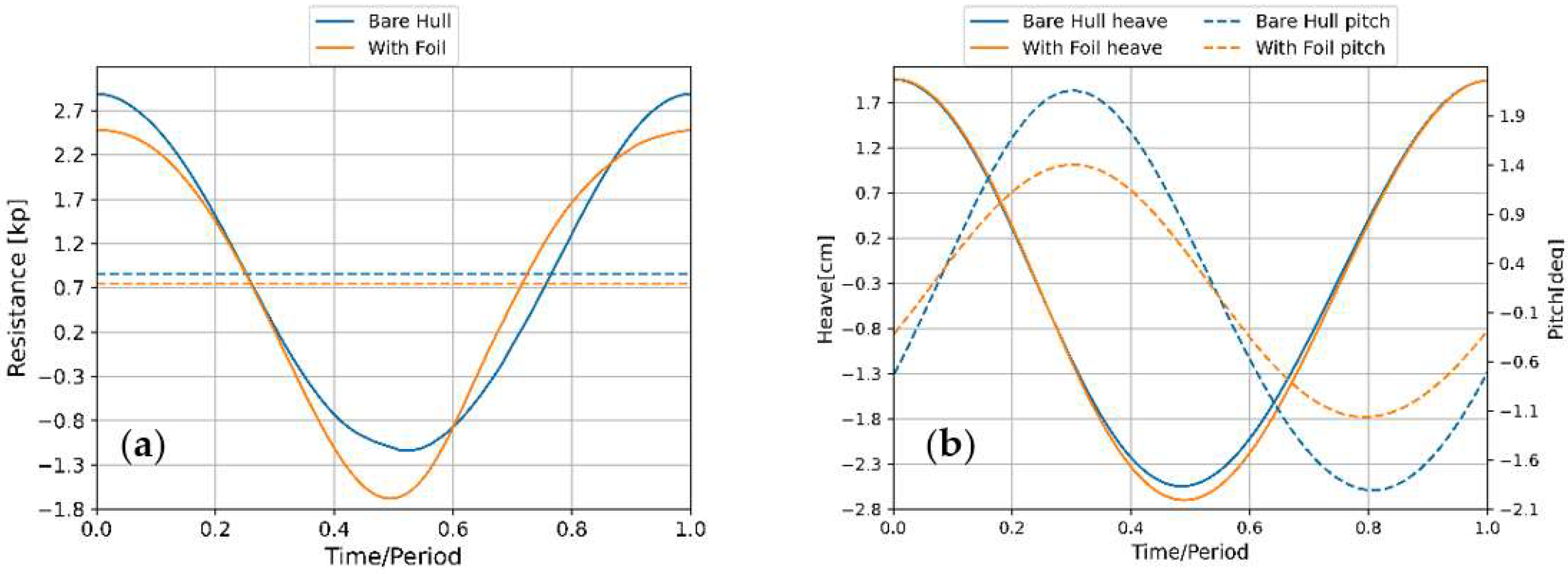
Jmse 10 00492 g013
Figure 14. Numerical results of (a) model resistance and (b) pitch and heave motions with and without the foil over one encounter period. In the left figure, the dotted line corresponds to the mean value of the model’s resistance. Wave frequency: f = 0.55 Hz. Wavelength to ship length: Lw/Ls = 1.62.
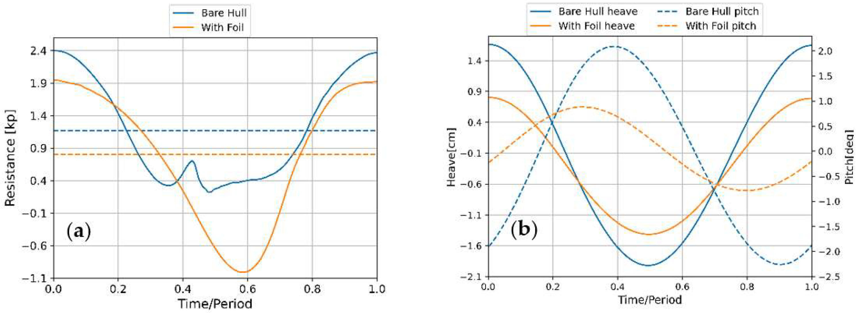
Jmse 10 00492 g014
Figure 15. Numerical results of (a) model resistance and (b) pitch and heave motions with and without the foil over one encounter period. In the left figure, the dotted line corresponds to the mean value of the model’s resistance. Wave frequency: f = 0.67 Hz. Wavelength to ship length: Lw/Ls = 1.09.
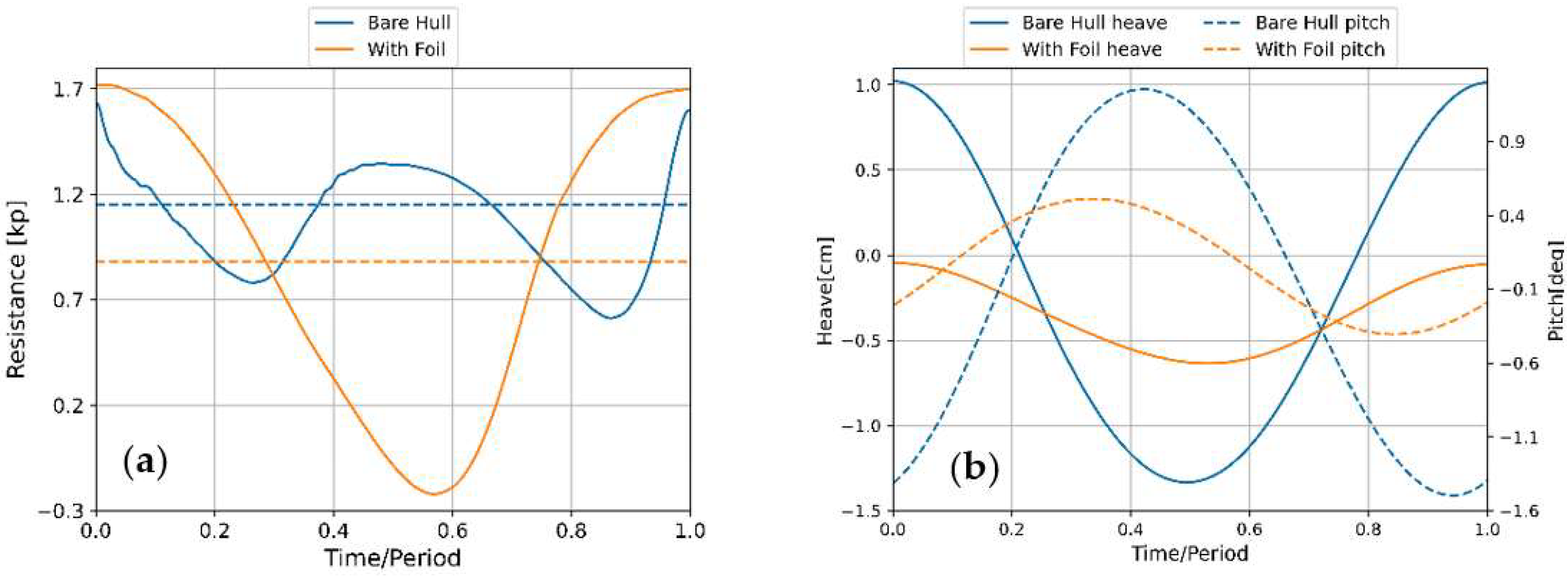
Jmse 10 00492 g015
Figure 16. Numerical results of (a) model resistance and (b) pitch and heave motions with and without the foil over one encounter period. In the left figure, the dotted line corresponds to the mean value of the model’s resistance. Wave frequency: f = 0.75 Hz. Wavelength to ship length: Lw/Ls = 0.87.
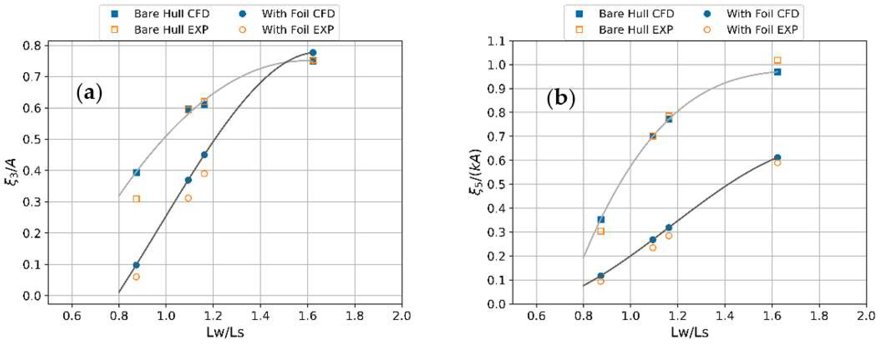
Jmse 10 00492 g016
Figure 17. Comparison between numerical and experimental results for regular waves with and without foil. The figures present the response amplitude operators for (a) nondimensional heave and (b) normalized pitch, where A is the wave amplitude, and k is the wave number.
Jmse 10 00492 g017
Figure 18. Iso-surface of the density field for ρm = 500 kg/m3 colored by the vertical coordinate. The two figures correspond to the heavier draft (T = 0.135 m) for an incident wave frequency of 0.67 Hz; (a) presents the bare hull case and (b) depicts the hull equipped with the static foil.
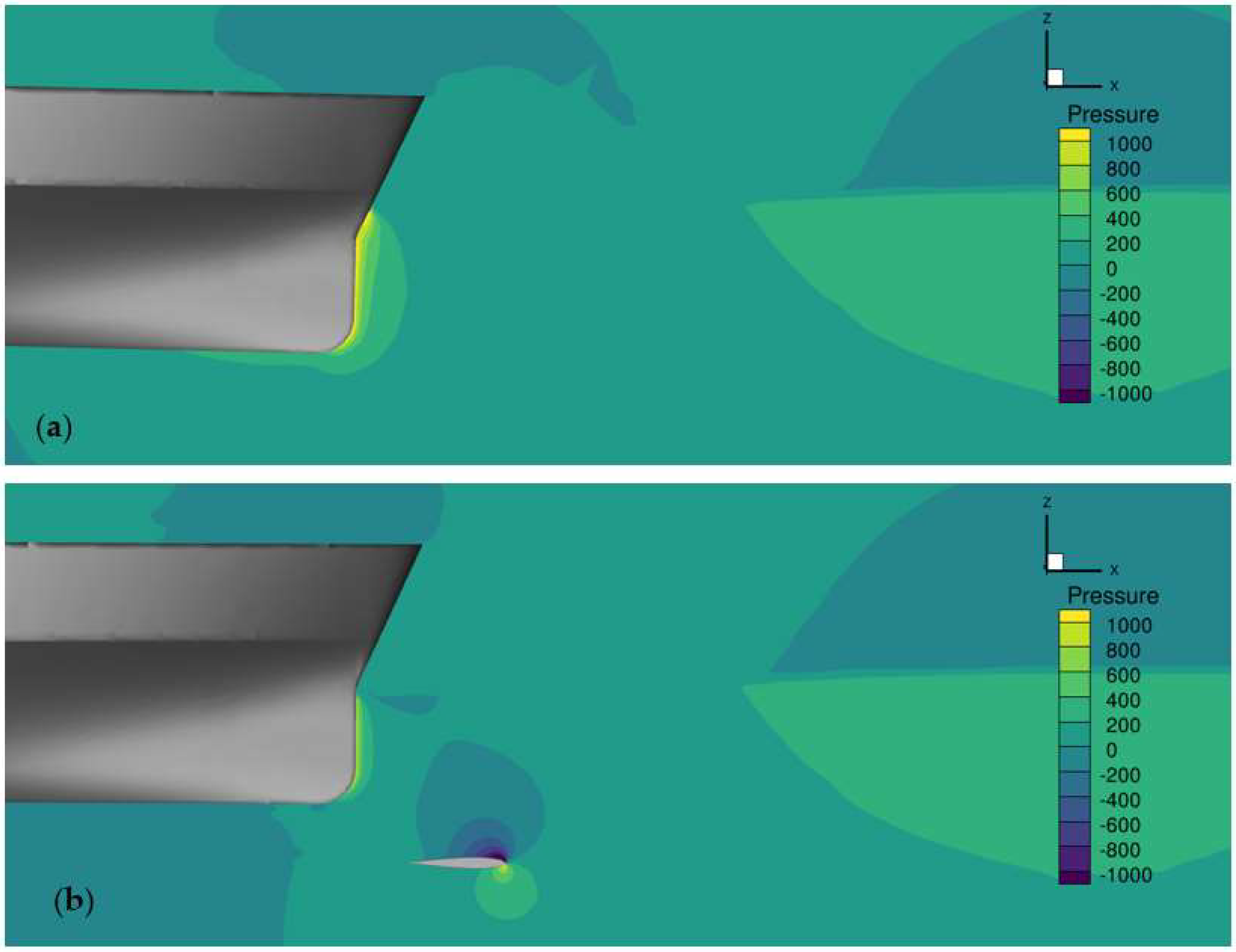
Jmse 10 00492 g018
Figure 19. Pressure field at the symmetry plane (y = 0 m) for the two configurations: (a) presents the base hull case, while figure (b) depicts the hull equipped with the static foil. The two figures correspond to the heavier draft (T = 0.135 m) for an incident wave frequency of 0.67 Hz.
Jmse 10 00492 g019
Table 1. Grid and time-step independency study.
Grid-Time-StepResistance (kp)Trim (deg)Sinkage (cm)
G3-Tref/25000.7040.0977−0.386
G2-Tref/25000.6870.0954−0.388
G1-Tref/25000.6820.0922−0.392
G2-Tref/5000.6860.0959−0.387
G2-Tref/2500.6860.0958−0.387
Table 2. Estimation of the spatial discretization error for the resistance calculations.
h1h2h3r21r32p φ e x t 21 e a 21 e e x t 21 G C I f i n e 21
0.04550.06160.08601.351.401.530.6740.73%1.26%1.56%
Table 3. Contribution of the individual components of the full configuration on the model’s resistance. Three different Froude numbers were examined for the T = 0.135 m draft.
Froude No.Total [kp]Hull [kp]Skegs [kp]Wing [kp]
0.250.8290.660.0770.092
0.220.6530.520.0610.072
0.1760.4310.340.0430.048
Table 4. Contribution of the individual components of the full configuration on the mode’s resistance. Three different Froude numbers were examined for the T = 0.125 m draft.
Froude No.Total [kp]Hull [kp]Skegs [kp]Wing [kp]
0.250.7880.620.0730.095
0.220.6140.480.0590.075
0.1760.4130.320.0420.051
Table 5. Experimental results for the static wing in various AoAs. All results regard the nominal speed of the vessel (Fn = 0.25 or Vnom = 1.42 m/s) in the case of the heavier condition (T = 0.135 m).
Angle of Attack [deg]Resistance [kp]Trim [deg]Sinkage [cm]
−3.11.031−0.159−0.198
−1.61.007−0.039−0.291
1.61.0280.264−0.494
01.0420.132−0.401
Table 6. Time-step independency study for the case study with regular waves. The table presents the mean value (   ·   ) ¯ and amplitudes (A) of the heave ( ξ 3 ), pitch ( ξ 5 ), and resistance ( A p ).
dt [s] ξ 3 ¯ ξ 5 ¯ R p ¯ A ξ 3 A ξ 5 A R p
0.0031.932.271.181.932.271.18
0.0021.792.191.101.792.191.10
0.0011.752.141.081.752.141.08
Table 7. Mean resistance per encounter cycle for the bare hull and foil configurations at considered wave excitations.
Wavelength to Ship Length Lw/LsResistance [kp]
Bare Hull
Resistance [kp]
with Foil
Gain (%)
0.871.1530.883+23.5
1.091.1650.801+31.2
1.161.1770.774+34.2
1.620.8540.747+12.5
Publisher’s Note: MDPI stays neutral with regard to jurisdictional claims in published maps and institutional affiliations.

