Article

Numerical and Experimental Investigation of the Performance of Dynamic Wing for Augmenting Ship Propulsion in Head and Quartering Seas

by
Kostas Belibassakis
*,
Evangelos Filippas
and
George Papadakis
School of Naval Architecture & Marine Engineering, National Technical University of Athens, 15780 Zografos, Greece
*
Author to whom correspondence should be addressed.
J. Mar. Sci. Eng. 2022, 10(1), 24; https://doi.org/10.3390/jmse10010024
Submission received: 15 November 2021 / Revised: 15 December 2021 / Accepted: 17 December 2021 / Published: 27 December 2021
(This article belongs to the Special Issue Energy Saving Devices for Ships)

Abstract

:
Flapping-foil thrusters arranged at the bow of the ship are examined for the exploitation of energy from wave motions by direct conversion to useful propulsive power, offering at the same time dynamic stability and reduction of added wave resistance. In the present work, the system consisting of the ship and an actively controlled wing located in front of its bow is examined in irregular waves. Frequency-domain seakeeping analysis is used for the estimation of ship-foil responses and compared against experimental measurements of a ferry model in head waves tested at the National Technical University of Athens (NTUA) towing tank. Next, to exploit the information concerning the responses from the verified seakeeping model, a detailed time-domain analysis of the loads acting on the foil, both in head and quartering seas, is presented, as obtained by means of a cost-effective time-domain boundary element method (BEM) solver validated by a higher fidelity RANSE finite volume solver. The results demonstrate the good performance of the examined system and will further support the development of the system at a larger model scale and the optimal design at full scale for specific ship types.

1. Introduction

Extensive research concerning flapping-foil thrusters, including numerical modeling and experimental verification, has shown that the above systems, operating under conditions of optimal wake formation, can achieve high levels of propulsive efficiency; see, e.g., ref. [1]. The flapping-foil motion involves two oscillatory motions, heave and pitch, with appropriate phase difference and a forward speed motion [2], with the most energy demanding motion being the heave oscillation. In real sea conditions, the ship undergoes moderate or higher-amplitude oscillatory motions due to waves. In this case, the ship motions could be exploited for providing the foil heaving motion free of cost, especially if the foil is located at the bow; see, e.g., refs. [3,4,5,6]. Moreover, in [7,8] the authors have developed a nonlinear boundary element method (BEM) approach and studied the active control of oscillating hydrofoils operating as unsteady thrusters augmenting ship propulsion in waves.
In the framework of Seatech H2020’s project entitled “Next generation short-sea ship dual-fuel engine and propulsion retrofit technologies” (https://seatech2020.eu/, accessed on 15 November 2021), a concept of symbiotic ship engine and the flapping thruster innovation is studied, that when combined, are expected to lead to a significant increase in fuel efficiency and emission reductions. The innovations will be characterized by high retrofitability, maintainability and will offer ship owners a return-on-investment due to fuel and operational cost savings. The proposed renewable energy-based propulsion innovation is based on the biomimetic dynamic wing, mounted at the ship bow to augment ship propulsion in moderate and higher sea states, capturing wave energy and producing extra thrust while damping ship motions. A first analysis concerning the combined performance of innovative biomimetic ship propulsion system in waves with ship engine and application to short-sea shipping has been presented by Belibassakis et al. [9]. Based on simplified ship and foil dynamics models, in conjunction with ship engine data, a short-sea shipping scenario in the North Sea for a passenger-car ferry and bulk carrier was presented, illustrating the complementary nature of dynamic wing and engine innovations. The results show that the additional thrust generated by the dynamic wing, in conjunction with the reduction of added wave resistance due to dynamic stabilization of a ship in waves, will enable the engine to operate in part-load without compromising vessel speed, resulting in an additional positive effect on its emission profile.
In the present work, the basic model developed for the simulation of the system performance in head and quartering waves is presented, including comparisons against detailed BEM and CFD predictions which are used for verification and optimization of the model parameters. Moreover, selected experimental results are presented from the tests of the tank-scale model of the biomimetic thruster with active control carried out in waves at the National Technical University of Athens (NTUA) towing tank using a ferry ship-hull model. The experiments demonstrate the performance of the examined system and provide useful data in order to validate the numerical prediction tools, and further calibrate the thrust-power coefficient charts which will be used for the calculation of the combined performance with the standard propulsion system and establish design requirements and methodologies to extend predictions to a large model scale that will be tested at sea. The results will finally support the design of a full-size wing, including strength, fatigue and service life considerations, as well as actuation and a mechanical wing-retractability system in calm and heavy weather conditions, in order not to add to the resistance and protect the system, respectively.

2. Augmenting Ship Propulsion System in Waves by Controllable Dynamic Wing

2.1. Ship Dynamics Coupled with Unsteady Flapping-Foil Thruster

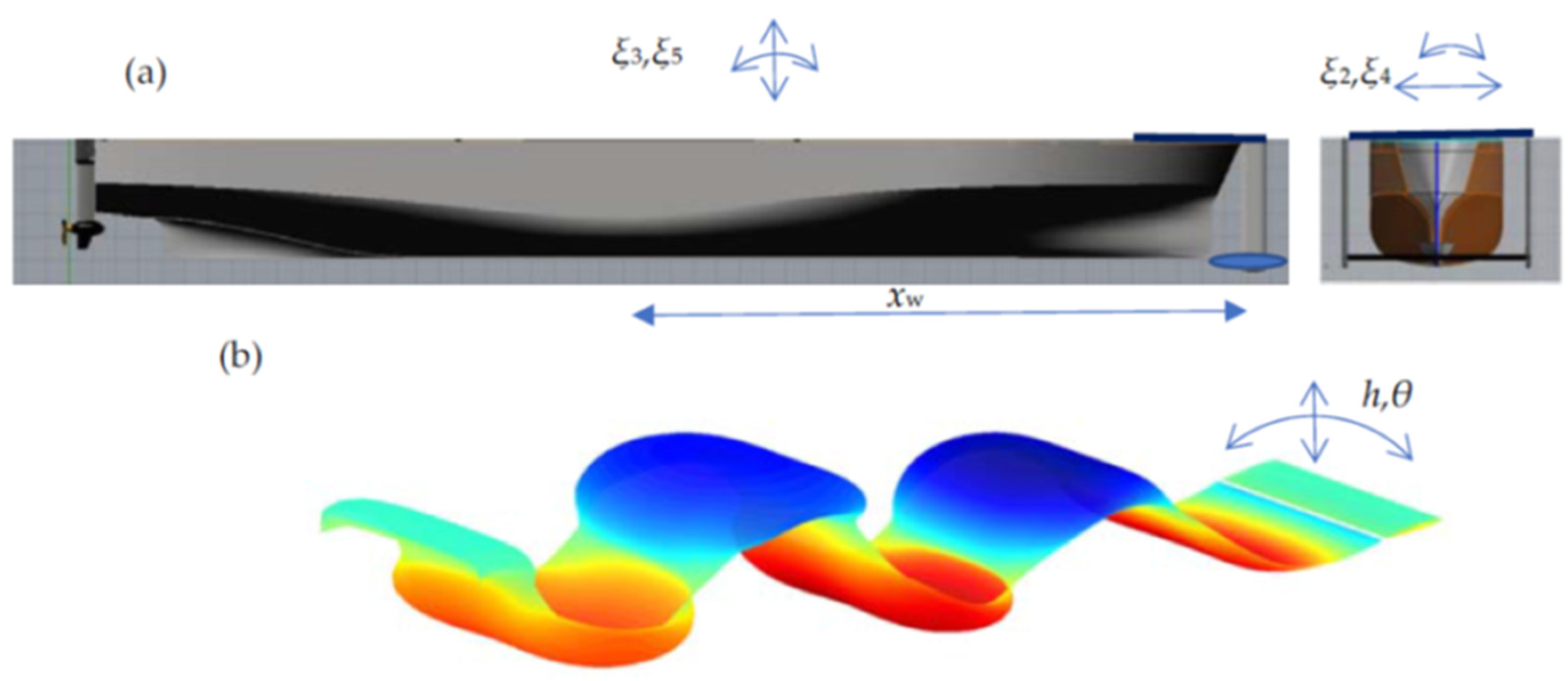
We consider a self-propelled ship traveling at constant forward speed U in waves propagating at an angle β with respect to the ship longitudinal axis, where 
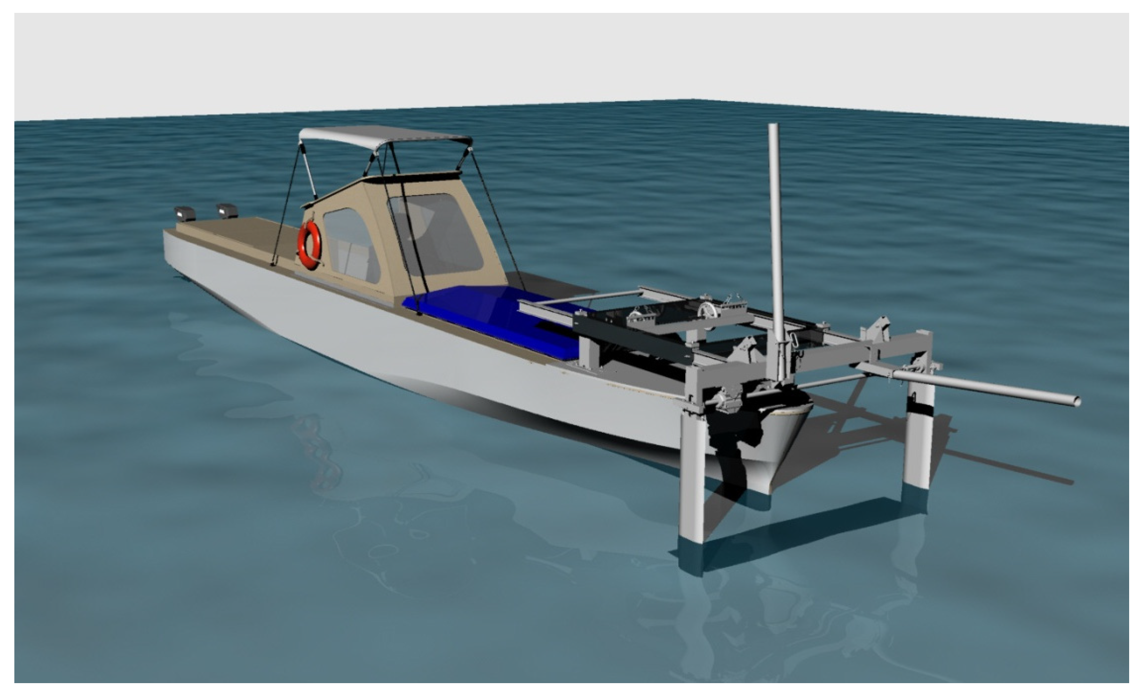
β = 180 deg corresponds to head incident waves. The ship is equipped with a dynamic wing arranged at the bow, as shown in Figure 1, which takes energy from the wave-induced ship responses. By enforcing a self-pitching motion controlled by a suitably designed system, it operates as a flapping thruster augmenting ship propulsion in moderate and more severe sea conditions.
We consider small-amplitude incident waves and ship responses, permitting application of the standard seakeeping model in the frequency domain to calculate the coupled heaving ( ξ 3 ) and pitching ( ξ 5 ) motion of the system (ship and foil) in the vertical plane, and the corresponding sway ( ξ 2 ) and roll ( ξ 4 ) transverse motion responses; see [3]. The flapping thruster is arranged at a forward station (xw) at the ship bow, and its vertical motion h is defined from the ship heave ξ 3 , pitch ξ 5 and roll ξ 4 responses, as follows:
h = h 0 + y w ξ 4 ,   h 0 =   ξ 3 x w ξ 5 ,
where h 0 is the vertical oscillation of the wing midchord section, x w denotes the longitudinal position of the wing axis of rotation and y w the transverse coordinate along the wingspan.
The dynamic wing is put in a flapping thruster mode by dynamically controlling its self-pitching motion denoted by θ. Following standard seakeeping analysis in deep-water harmonic waves, the dynamics of the system on the vertical and transverse plane, respectively, are described as follows (see [3,10,11]):
D 33 ξ 30   + D 35 ξ 50 = F 30 + X 30 ,   D 53 ξ 30 + D 55 ξ 50 = F 50 + X 50 ,
D 22 ξ 20   + D 24 ξ 40 = F 20 + X 20 ,   D 42 ξ 40 + D 44 ξ 40 = F 40 + X 40 ,
where ξ k 0   ,   k = 2 , 3 , 4 , 5 , are the complex amplitudes of ship swaying, heaving, rolling and pitching oscillations. In the present work, the effect of the swaying and rolling motion on the foil generation loads X 20 , X 40 has been considered very small in comparison with the Froude–Krylov and diffraction component and has been approximately neglected. The coefficients D k are defined as follows:
D k = ( ω e n 2 ( a k + m k ) + i ω e n b k + c k + p k ) ,
where a k and b k ,   k , = 2 , 3 , 4 , 5 , are the added mass and damping coefficients, m k are components of the mass-inertia matrix of the system (ship and wing), c k denotes the matrix of hydrostatic coefficients and p k are Coriolis terms; see, e.g., Refs. [6,7]. Furthermore, the encounter frequency is
ω e n = ω + k U cos β ,
where k = ω 2 / g is the wavenumber of the incident waves and ω is the absolute wave frequency. Moreover, F k 0 ,   k = 2 , 3 , 4 , 5 denote the Froude–Krylov and diffraction wave loads, respectively. In the above model, the coupling with the flapping thruster dynamics is achieved through the terms X k 0 ,   k = 2 , 3 , 4 , 5 which are complex amplitudes of excitation due to the wing, and are functions of heaving-pitching ( ξ 3 , ξ 5 ) and swaying-rolling ( ξ 2 , ξ 4 ) responses of the ship. The vertical force and moment consist of two parts:
X k 0 = X k 0 , A ( ξ 3 , ξ 5 ) + X k 0 , B ( φ I N C ) ,   k = 2 , 3 , 4 , 5 ,
dependent on the oscillatory ship responses and on the incident wave field φ I N C = Λ exp ( k z + i k x ) , where Λ is a constant coefficient involving the incoming wave height and period; see [3] for details concerning the definition of the above quantities.
In the sequel, we will briefly describe the approach that is used in order to analyze the wing forces and moments using the unsteady thin hydrofoil theory. Beginning with the kinematics of the flapping foil, the effective angle of attack is approximately given by
α ( t ) ξ 5 ( t ) + ε ( t )   + 1 U φ I N C z + y w ξ 4 θ ( t ) ,
where θ ( t ) denotes the angle of the self-pitching motion of the foil. In Equation (7), the effect of wing’s vertical oscillation on the angle of attack is ε ( t ) = tan 1 ( U 1 d h 0 ( t ) / d t ) , where h 0 ( t ) denotes the oscillatory motion of the ship at its centerplane and at the longitudinal position x w i n g of the foil; see Figure 1. For small vertical oscillatory velocity compared to the ship’s speed, the following approximation can be used: ε ( t ) U 1 d h 0 ( t ) / d t . The self-pitching motion is selected to be actively controlled by a simple proportional law based on the angle ε , i.e., θ ( t ) = w   ε ( t ) , where w stands for the control parameter. Thus, the following expression is obtained for the angle of attack of the incident flow on the foil sections:
α ( t ) = ξ 5 ( t ) + ( 1 w )   ε ( t ) + 1 U φ I N C z + y w ξ 4 .
Since, in the band of frequencies of interest, the wave field is a slowly varying quantity along the span of the foil, it is approximated by its value on the midchord plane, which in the considered arrangement is the centerplane of the ship. It is worth noticing here that the above set-up also includes the case of the bow wing operating in static mode θ = const, which resembles the cases of hull vane and bow static wings that have also been found to be beneficial concerning resistance reduction of traveling ships; see e.g., [12].
Assuming a relatively large aspect ratio of the flapping thruster, the unsteady lifting line theory is used to analyze foil excitation. Under the additional consideration of small and moderate Strouhal numbers, S t r = ω e n c h 0 / ( π U ) and reduced frequency k r e d = ω e n c c / ( 2 U ) , where c is the foil midchord length, the calculation of forces is based on spanwise integration of sectional lift forces and moments X k 0   ,   k = 2 , 3 , 4 , 5 , as presented in detail in [3,7]. The above analysis also provides data concerning the variation to the system coefficients δ a k , δ b k , k = 2 , 3 , 4 , 5 , in the left hand side of Equations (2)–(4) due to the operation of the flapping foil. Furthermore, expressions are obtained concerning the most significant incident wave-field-dependent foil forces X k 0 , B ( φ I N C ) , as follows:
X 30 , B = G   ( i ω / U )   exp ( k d + i k x ) ,   X 50 , B = G   x w i n g   ( i ω / U )   exp ( k d + i k x ) ,
where d is the foil submergence depth and G is a factor defined from the geometrical parameters of the wing. More details concerning the modeling can be found in [3], and its application in combination with BEM, including free-surface effects, in [7] and validation by comparison to BEM and CFD in [8].

2.2. Experimental Investigation of the Model

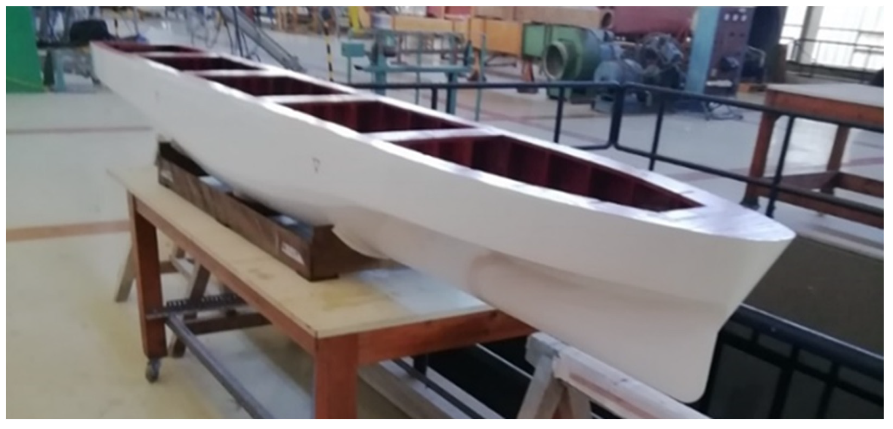
For the verification of the present method, a new ship model corresponding to a ferry hull of length between perpendiculars LBP = 3.3 m, with main dimension ratio: LBP/B = 7.67, B/T = 3.3 and hull coefficients Cb = 0.45, Cwl = 0.73, Cm = 0.82, has been designed, constructed and tested at the NTUA towing tank without and with the operation of a dynamically controllable flapping thruster arranged at the bow; see Figure 1 and Figure 2. The dimensions of the NTUA towing tank are: length 100 m, breadth 4.6 m and maximum depth 3 m. Moreover, the maximum carriage speed is 5 m/s. The model was made out of wood and prepared for testing at two selected drafts, B/T = 3.18 and B/T = 3.44. The foil is constructed by poly (vinyl chloride) (PVC), polished and painted. The foil planform shape is orthogonal; its span is s = 0.50 m with a span to chord ratio of s/c = 4 and thus, its aspect ratio is AR = 4 and the wing planform area is Sw/BT = 1.17. The foil sections are symmetrical NACA0012. The model is painted white and marked with the two waterlines used in the tests in order to provide a reference in the photographs; see Figure 2.
Moreover, the center of flotation of the ship is LCF/L = −0.05 (aft midship) and the metacentric radius BML/L = 1.9. The vertical coordinate of the center of buoyancy is KB/L = 0.024 (from BL) and its longitudinal position LCB = −0.024 L. We consider that the ship trim and heel angle are zero and thus, the longitudinal center of gravity is the same as the center of buoyancy, i.e., XG/L = −0.024 (aft midship) and YG = 0. The vertical center of gravity is KG/T = 0.2(from BL). Furthermore, the longitudinal metacentric height is G M L B M L . Finally, the radii of gyration about the x-axis and y-axis, respectively, are taken Rxx/B = 0.25, Ryy/L = 0.2. The foil is located at a distance xwing/L = 0.5, with respect to the midship section, and vertically at a submergence depth d/T = 1.6.
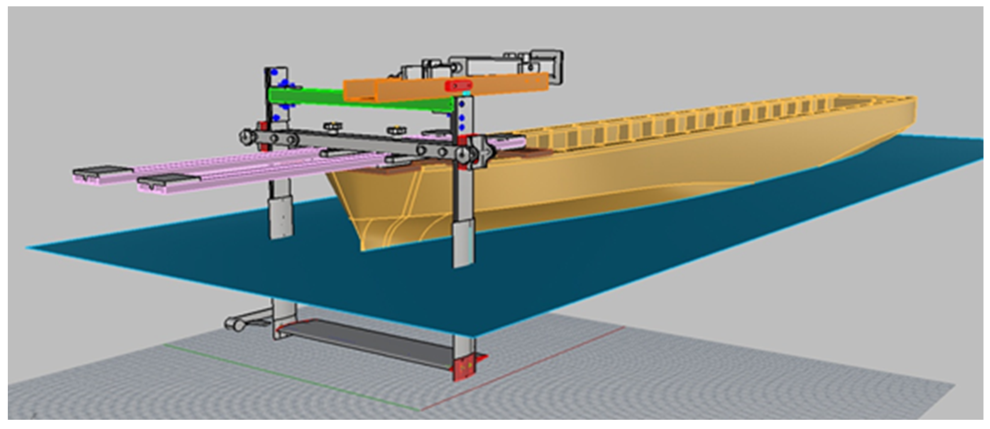
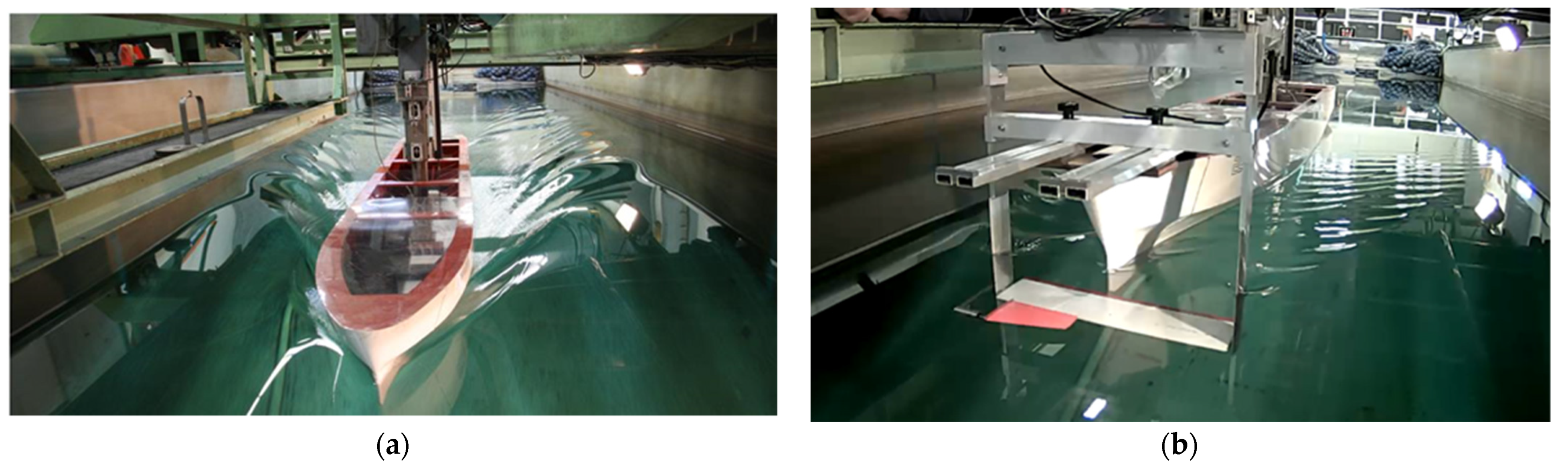
The model is tested without and with the operation of a biomimetic dynamic wing. The dynamic wing system is designed to be arranged at the bow of the ship, as shown in 
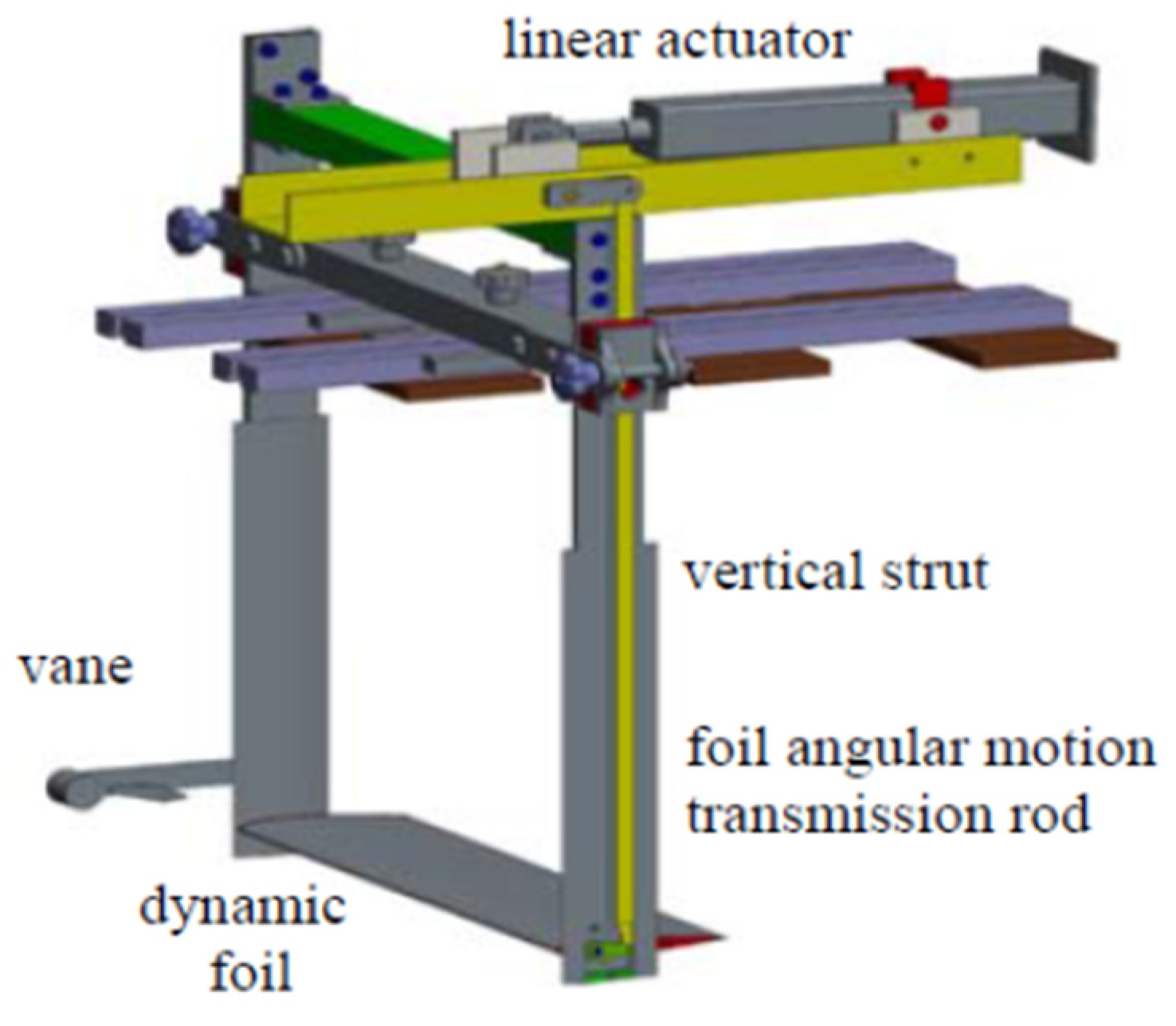
Figure 3. For the operation and powering of the flapping thruster a servo motor coupled to a linear actuator is used, as presented in Figure 4. The pivot axis of the wing is located at its hydrodynamic center, and the power required for the dynamic pitching of the foil is found to be negligible compared with the effective horsepower associated with the resistance of the ship model. The angular oscillatory motion of the flapping foil is transmitted by means of two rods arranged inside the vertical struts that are used to support the system; see Figure 4. The latter ensures that the motion is transmitted very accurately, as instructed by the control system.
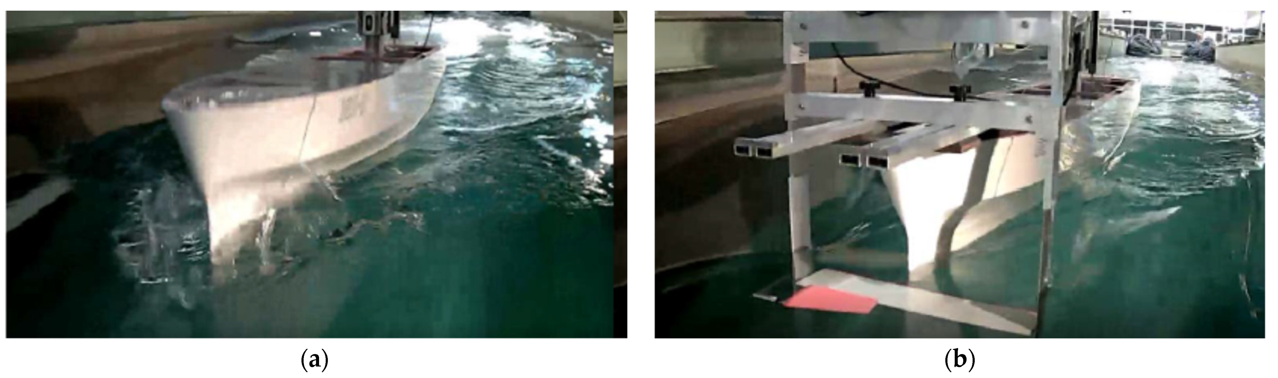
Using the above model, a series of experiments concerning calm water resistance at the specific drafts have been performed, as shown in Figure 5. Moreover, tests in harmonic and irregular waves are performed, and the responses, including motions and total wave resistance, are measured, as shown in Figure 6. It is worth mentioning here that the breadth of the model is less than 10% of the breadth of the tank, indicating that block effects are not important. Indicative results are reported below, demonstrating the performance of the examined system.
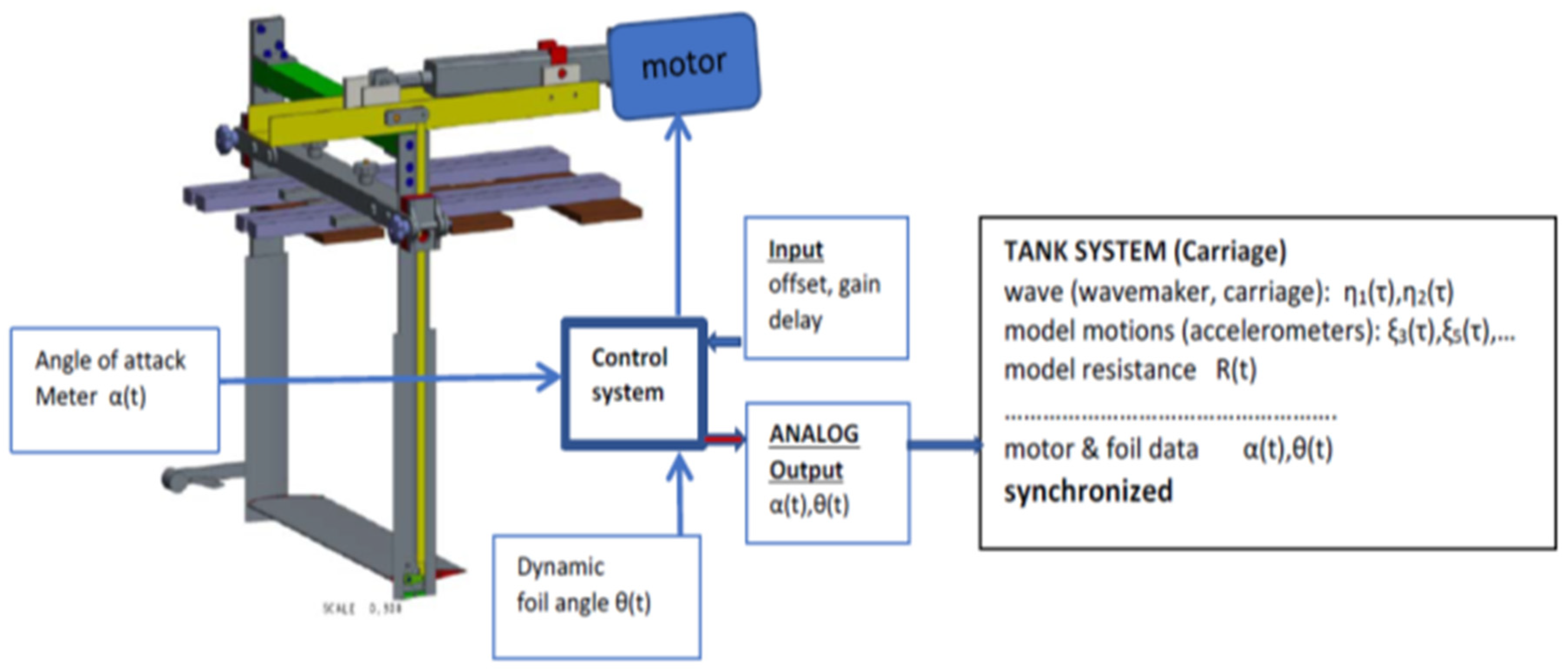
The control system (CS) setting the self-pitching motion of the foil is based on the reading of the angle of attack of the flow in front of the dynamic wing, using the angle of attack meter (vane) which is shown in Figure 7.
The control system accepts the following input data: O = offset, G = gain, D = delay and performs the following functions:
(a)
The dynamic angle of attack is measured using a potentiometer providing input α(t) to the CS.
(b)
The foil angle is measured by using a potentiometer providing input θ(t) to the CS.
(c)
The CS instructs the motor to rotate in order to force the linear actuator and rotate the crankshaft, oscillating the vertical rods and transmitting the angular motion θ(t) to the foil which is set equal to:
θ ( t ) = G a ( t D ) + O .
The output is synchronized with the towing tank acquisition system, providing simultaneous records of the following data for given tank carriage speed (model speed):
(a)
Wave elevation from the wavemaker and near the tank carriage (near the vessel): η1(t), η2(t);
(b)
Ship model motions (heave and pitch of the hull from tank accelerometers): ξ3(t), ξ5(t);
(c)
The model resistance in the presence of waves with the dynamic foil in operation: R(t);
(d)
The angle of attack α(t) and the foil angle θ(t).
The input signal from the angle of attack meter (vane) is low pass filtered as follows:
-
0–6 Hz, Gain = 1/ripple 2.75 dB and
-
18–104 Hz, Gain = 0/Actual attenuation −43 dB.
The sampling rate is set to 208 Hz.
The CS is a custom design board based on an ST microelectronics STM32F429 ARM mcu, running at 168 MHz. The firmware is based on FreeRTOS real-time operating system. The control board provides the following functions:
-
Analog input for the AoA sensor. Oversampled at 2048 Hz and low pass filtered at 6 Hz.
-
Digital serial output to Animatics/Moog brushless servo motor (actuator).
-
5 × 12 bits spare analog outputs for monitoring.
-
3 × 12 bits spare analog inputs for interfacing auxiliary sensors
-
3D gyroscope and 3D accelerometer.
-
3D magnetometer and pressure sensor.
-
GNSS and WiFi/Bluetooth.
-
GPRS/2 G/3 G.
-
CAN Bus interface and uSD card for data acquisition.
The firmware implements various control and RTK kinematics algorithms such as:
-
Quaternion estimation and Euler angles.
-
Linear acceleration and speed.
-
Assisted global positioning and real-time spectral analysis.
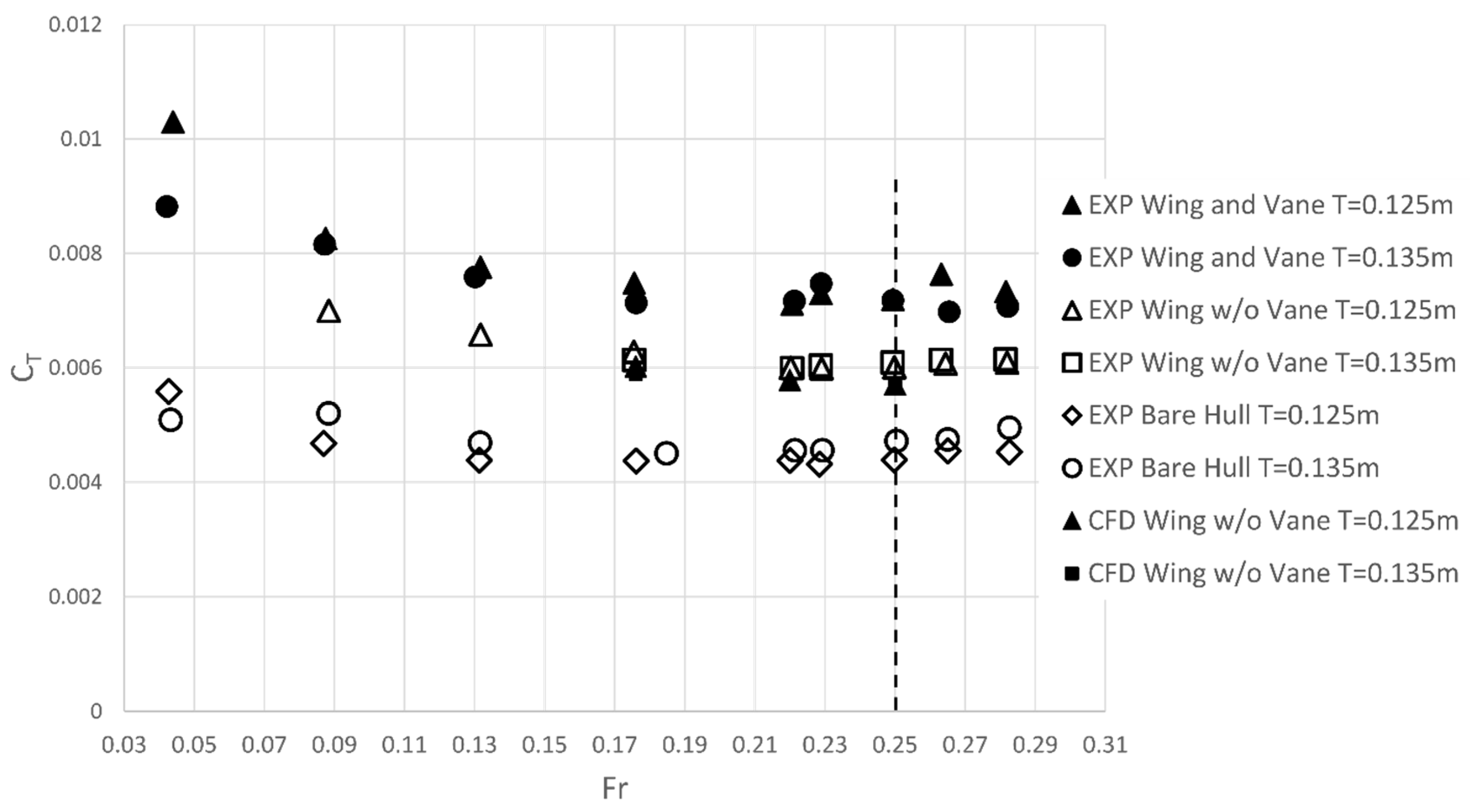
The calm water resistance of the model at the two drafts tested, without and with the flapping thruster, as depicted in Figure 5 and Figure 6, is measured and indicative results are shown in Figure 8, where the total resistance coefficient C T = R t o t / ( 0.5 ρ S U 2 ) is plotted against the Froude number F r = U / g L B P . More specifically, R t o t is the total resistance and U is the model towing speed, ρ is the water density and S denotes the wetted area of the ship model at each draft, respectively. The design speed corresponds to Froude number Fr = 0.25 indicated by a vertical dashed line in Figure 8. In this condition, an increase of the calm water resistance of about 60% is observed due to the presence of the foil and the supporting system, including the two vertical struts and the vane. To quantify the increase in the total resistance due to the vane, additional experiments have been conducted without it. To supplement the measurements, numerical simulations using an in-house finite volume CFD solver (see Section 3.2) are performed. The vane is also omitted from the numerical simulations in which the hull, wing and struts are modeled.
As indicated in Figure 8, almost one third of the above increase in resistance is found to be due to the contribution of the vane. This is evident both in the measurements as well as in the numerical predictions, which are found to be in good agreement with the experimental data. Since the vane is used for the control of flapping thruster, it does not need to scale with the rest of the model. Consequently, the contribution of the vane to the total resistance is expected to be eliminated at larger scales, where the dimensions and size of the vane will remain of the same order, as in the tank experiments. The resistance due vane viscous losses become negligible in full-scale applications, for which an optimization procedure will be used for the design of the supporting struts and chord and span of the foil. The latter approach will minimize the combined drag, taking into account the required size and space for the transmission system, and will be the subject of subsequent work.
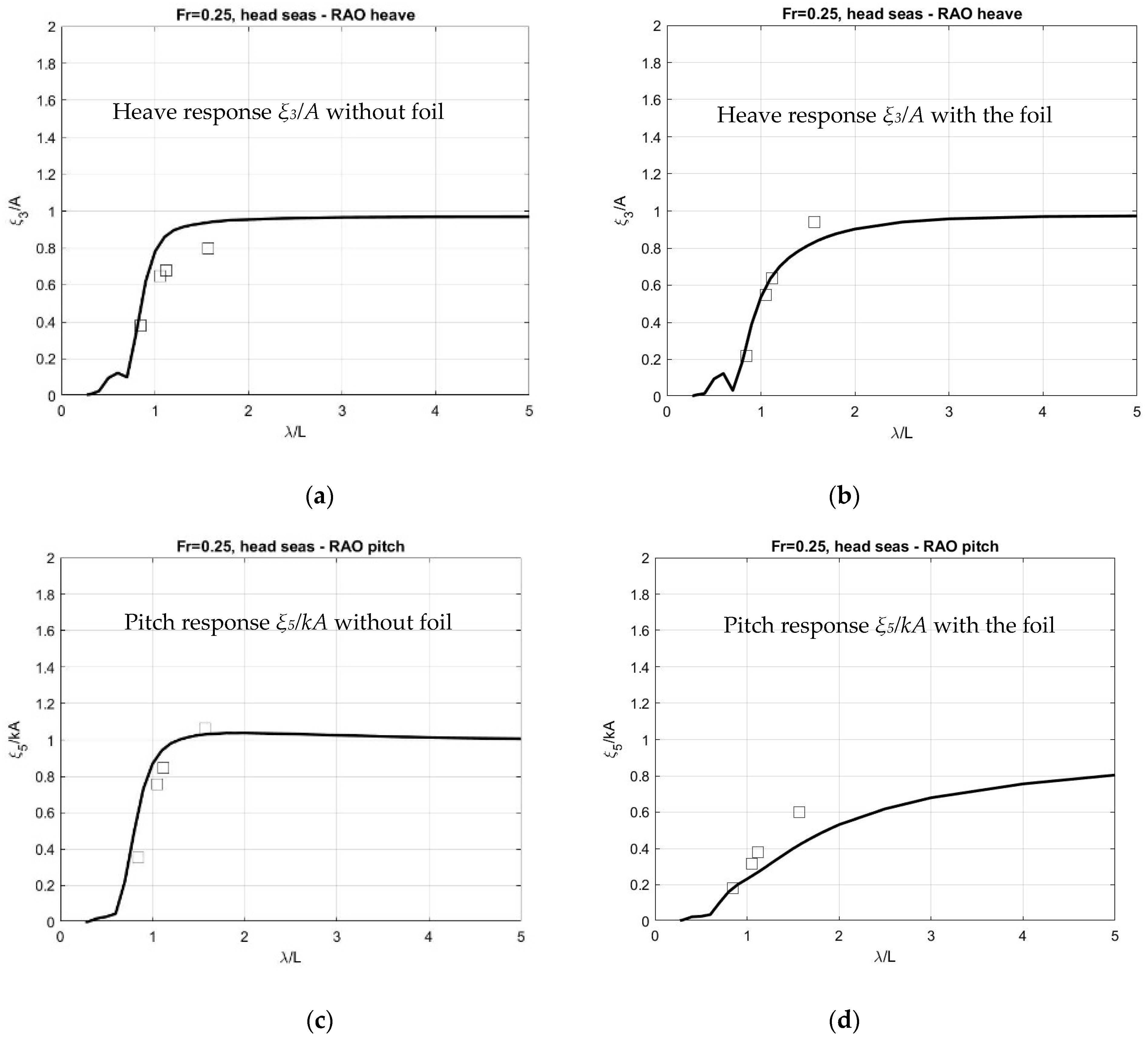
Measured data concerning the ship motion responses with and without the operation of the dynamic wing are shown in Figure 9 in harmonic head waves, with and without the operation of the dynamic foil, for Froude number Fr = 0.25, and the smaller draft of the ship. In the same figure, the predictions obtained by the present numerical model are also plotted using lines.
It is observed that the operation of the foil leads to a significant reduction of ship hull motion responses, which is equivalent to a reduction of added wave resistance and an overall increase of propulsion performance in waves. This is also evident from the pictures in Figure 6, which correspond to the same forward speed of the model at Fr = 0.25 and same head wave conditions. It is clearly observed that the motion responses are reduced at a great extent due to the operation of the foil. The same findings have also been observed in the case of the ship responses in irregular waves.
More details concerning the enhancement of the performance by the operation of the dynamic foil are provided in Table 1. The table data are presented as obtained from the operation of the system in forward speed of the model at Fr = 0.25, in harmonic head incident waves of various frequencies around the resonance conditions for a given wave amplitude (A/L = 1%). Each line provides the enhancement of propulsive performance for the corresponding value of the gain G by the control system (with offset and delay set equal to zero).
The percentage of performance enhancement is calculated with respect to the total resistance of the ship without the dynamic wing traveling at the same speed in head waves of the same characteristics, which includes the calm water resistance and the added resistance due to the waves the at the same conditions. It is clearly observed that for an extended frequency band around the resonance conditions of the ship, a significant enhancement of performance is achieved. The latter could reach the level of 15–30%, with the larger values indicated in the column Table 1 by using an asterisk, achieved if the penalty due to resistance increase by the vane is eliminated, as it is expected to happen at larger scales, and could be further optimized by the design of the supporting struts.

2.3. Modeling the Flapping Thruster Performance in Irregular Waves

Based on the data concerning the kinematics of the flapping thruster, as obtained from the seakeeping responses of the system, the performance of the system in random waves is calculated. For the studied ship speed, although the Froude number based on the length of the ship is F r = U / g L = 0.25 , the corresponding one based on the root chord c of the foil is F f o i l = U / g c = 1.3 .
We consider irregular waves described by a frequency spectrum S ( ω ) in the earth-fixed frame of reference and thus, the spectrum in the frame of reference moving with the foil forward speed U is
S U ( ω e n ) = S ( ω ) d ω d ω e n ,   with   d ω = d ω e n ( 1 2 ω U g cos β ) 1 .
Using the response amplitude operator concerning the vertical foil motion at the centerplane R A O = ξ 3 x w i n g ξ 5 at the position xwing of the wing, we obtain the corresponding spectrum describing the foil vertical motion as
S f o i l U ( ω e n ) = S U ( ω e n )   | R A O f o i l ( ω e n ) | 2 .
Next, the vertical motion of the flapping thruster is simulated by using the random-phase model by discretizing the encounter frequency band into a large number of bins of width δ ω and the corresponding centers at discrete frequencies ω e , n , as follows:
η ( t ) = n η n cos ( ω e , n t + k x w i n g + ε n ) ,   where   η n = 2 S f o i l U ( ω e , n ) δ ω e ,
where ε n are random phases uniformly distributed in [ 0 , 2 π ) ; see, e.g., refs. [11,13]. Moreover, the rotational motion of the flapping wing about its pivot axis is considered. The latter motion is defined to be negative in the clockwise direction, and the corresponding pivot point is located at a distance of x R = c / 3 from the leading edge of the foil. Finally, the self-pitching motion of the foil is set by a using a proportional control law based on the velocity of its vertical oscillatory motion as
θ ( t ) = w   tan 1 ( 1 U d h 0 ( t ) d t ) ,
where 0 < w < 1 is the control parameter; see [3,8]. The incident frequency spectrum is represented in the present work by using the Bretschneider model
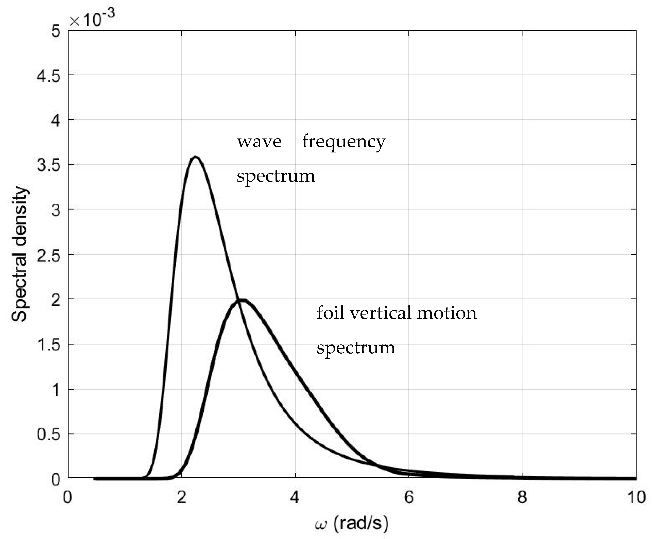
S ( ω ) = 1.25 4 ω m 4 ω 5 H s 2 e p x ( 1.25 ω m 4 ω 4 ) ,
as plotted in Figure 10, for significant wave height Hs/L = 0.03 and peak period T p U / L = 0.7, where it is also compared with the corresponding spectrum of foil vertical motion in the ship frame of reference traveling at Fr = 0.25 (solid line), in case of head incident waves (β = 180°), as obtained from Equation (12) for head seas.
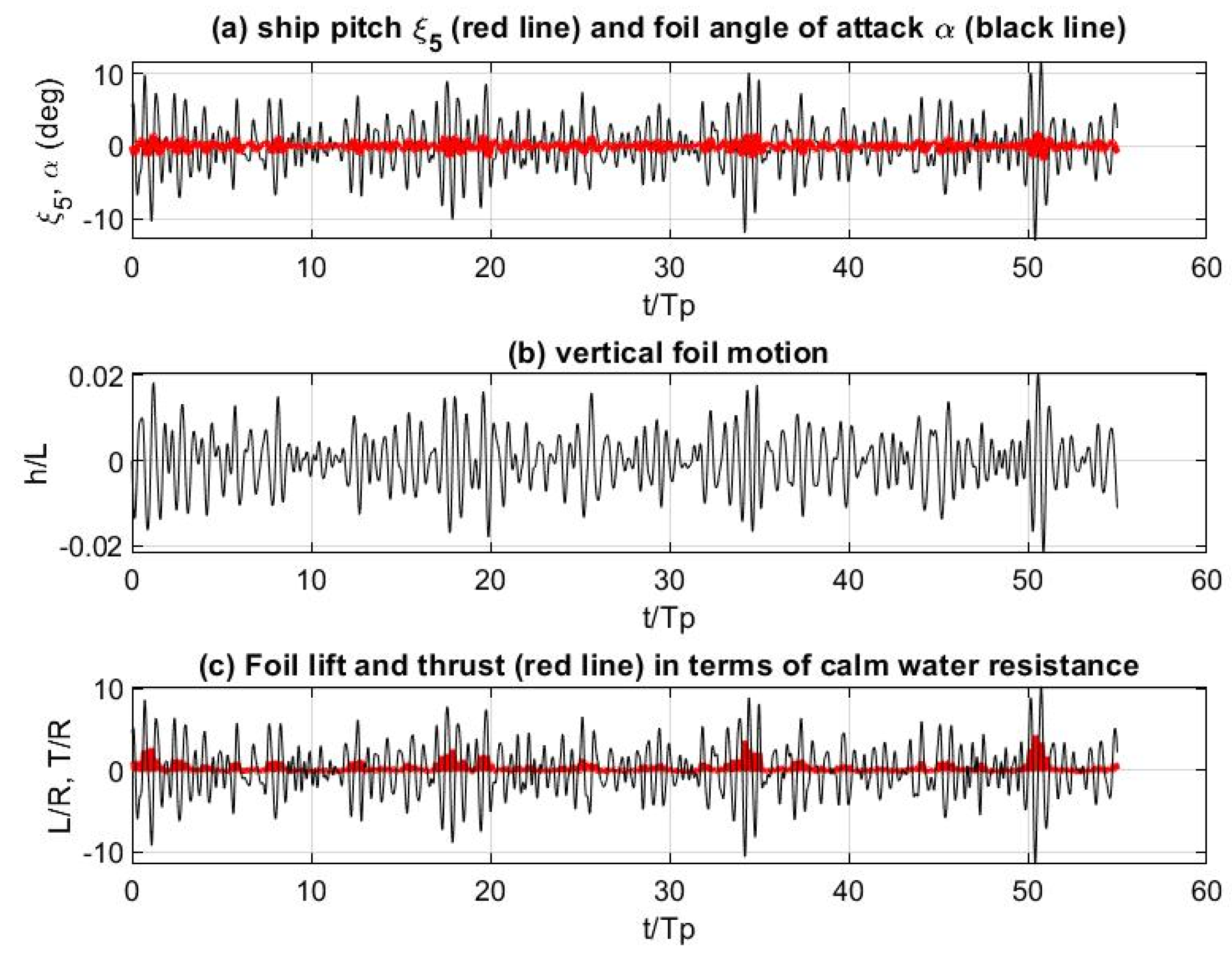
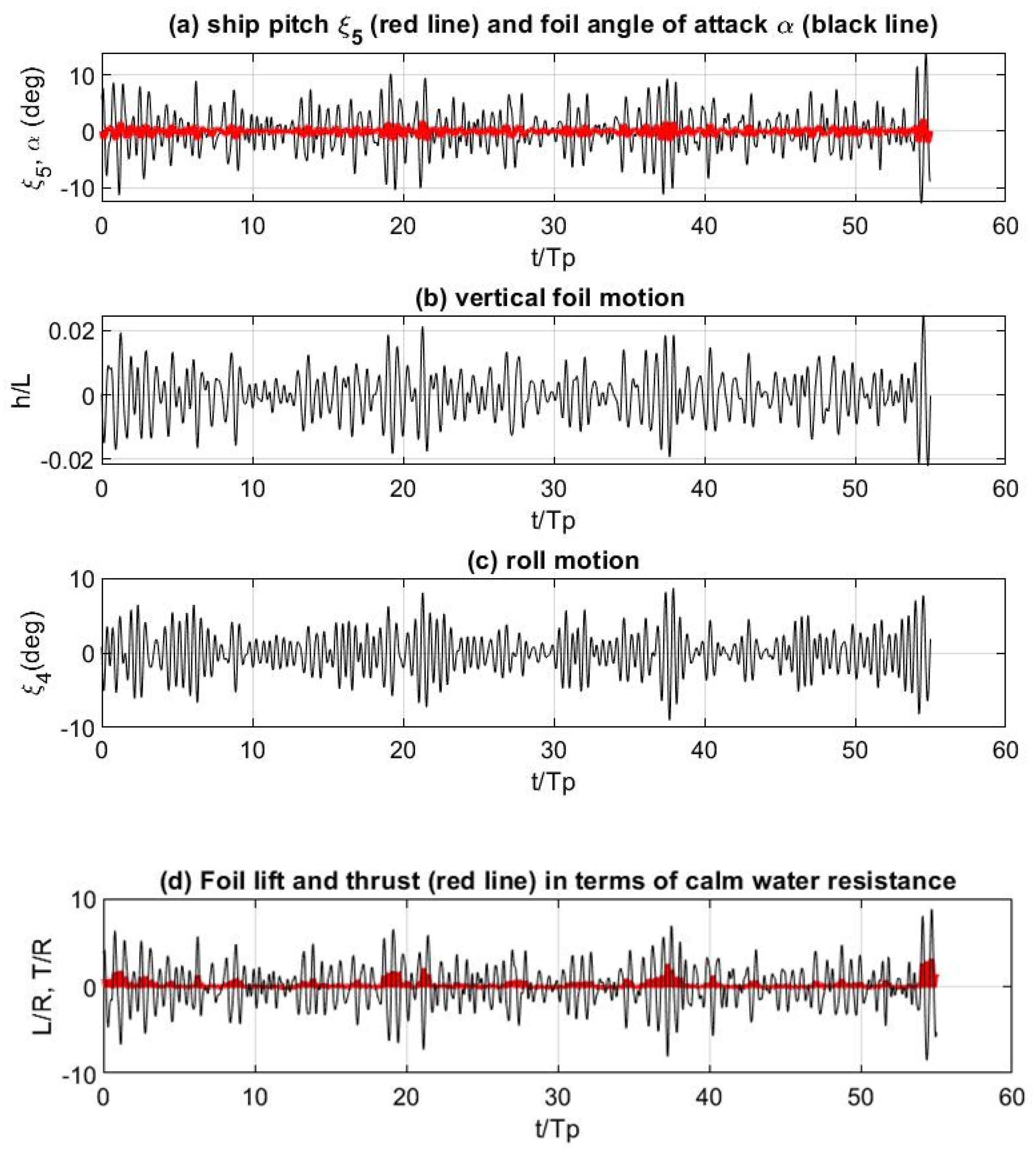
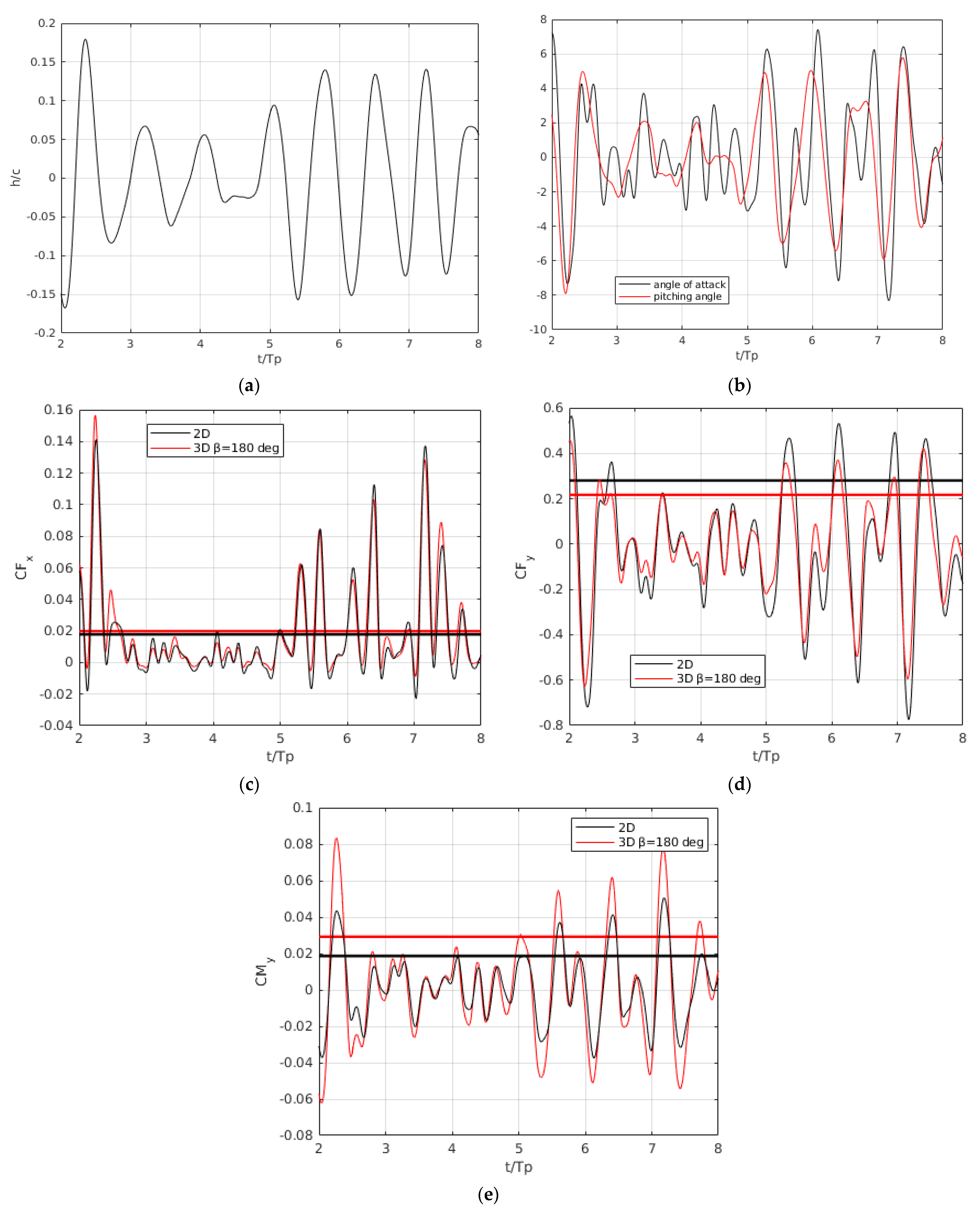
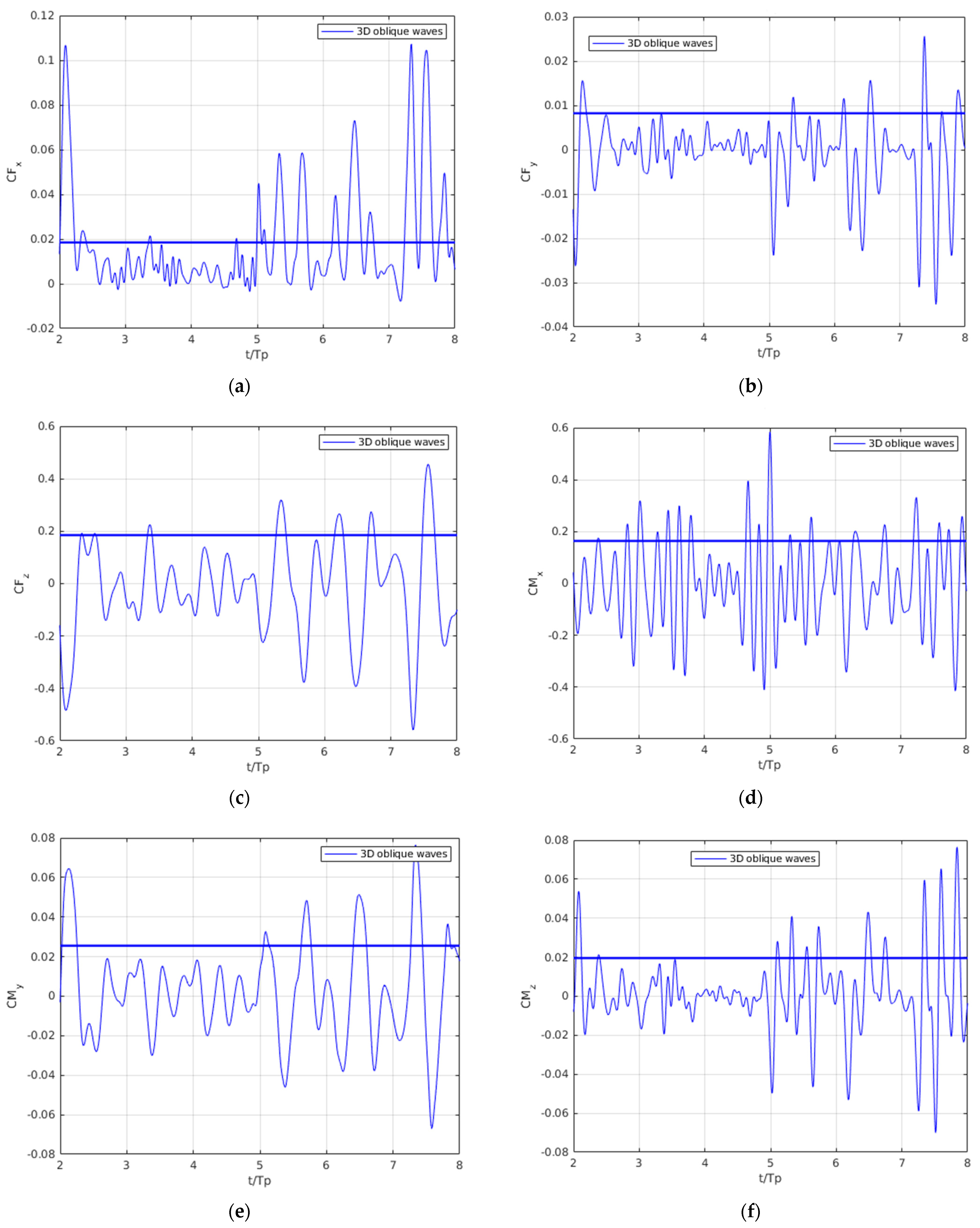
As an example of an application, in Figure 11 and Figure 12, selected results are presented in the case of the studied ferry ship model traveling at F r = U / g L = 0.25 with the operation of a flapping thruster at the bow, as schematically shown in Figure 1, for wave direction β = 180° (head waves) and β = 150° (quartering seas). In the top subplot of Figure 11, the ship pitching motion and the dynamic foil angle of attack in degrees are plotted, the latter being calculated by setting the self-pitching motion of the foil in proportionality with the angle of attack of the incident flow. In the middle subplot, the foil vertical motion is plotted normalized with the ship length, and in the lower subplot the dynamic foil lift force is shown by using a black line and the thrust force by a red line, respectively, both normalized with respect to the calm water resistance of the ship without foil. Similar results are plotted in Figure 12 for the same configuration, but in obliquely incident waves (β = 150°) corresponding to the same spectrum as before, where also in this case, roll motion is excited and its prediction by the present model is included in the third subplot of Figure 12.
In the examined conditions, the long-term average thrust offered by the dynamic foil is found to be of the order of 15–25% of the calm water resistance of the bare hull at the same speed, with the higher value corresponding to head waves. It is estimated that almost half of the above gain is due to the reduction of ship responses from the stabilization offered by the dynamic wing and the respective drop of the added wave resistance, while the other half part is due to the development of thrust by the flapping thruster, which by the appropriate control is put in fish-propulsion mode.
The above results are exploited for the calibration and verification of the more accurate numerical BEM and CFD tools developed for the design and analysis of the studied system supporting calculation at larger model scales and finally for the full scale, and details will be presented in the next sections.

3. Numerical Modeling of the 3D Flapping-Foil Thruster in Quartering Seas

Using the responses of the system, the kinematics of the flapping thruster are obtained, permitting the detailed study of its performance in random head waves by cost-effective BEM and high-fidelity RANSE solvers presented briefly in Section 3.1 and Section 3.2, respectively. The computational tools are direct extensions in 3D of the 2D models presented in detail in [8]. Moreover, 3D versions of the numerical methods exploited here have been presented in cases of foils operating at greater submergence depth from the free surface in [14].

3.1. Time Domain 3D BEM Model with Viscous Corrections

The oscillating lifting body is represented by a moving boundary D B ( t ) , with respect to the earth-fixed frame of reference. The seabed boundary is denoted with D H . The boundary is supposed to be smooth everywhere except at the trailing edge of the foil. Moreover, the wake of the body is modeled by another deformable boundary D W ( t ) , whose length grows, emanating continuously from the body sharp edge. A Cartesian coordinate system is introduced with x 3 -axis pointing upwards, x 2 -axis and x 1 -axis lying on the still free-surface plane, with x 1 -axis at the direction of body’s forward motion.
The linearized free-surface boundary conditions are imposed and are satisfied on the mean free-surface level. However, the present method has been extended to the nonlinear version and more details can be found in [15]. Due to linearization of the problem we can decompose the total potential to the incident wave potential Φ I which is known, and the disturbance potential Φ . The disturbance wave potential satisfies the Laplace equation in the interior of the domain supplemented by the body boundary condition
n Φ ( x ; t ) = b ( x ; t ) ,   x D B ( t ) ,   with   b ( x ; t ) = V B ( x ; t ) n B ( x ; t ) n Φ I ( x ; t ) ,
and the hard bottom no-entrance condition.
Moreover, the linearized dynamic and kinematic boundary conditions are given here:
t Φ ( x F , η ; t ) = g η ( x F ; t ) ,   x D F ( t ) ,
t η ( x F ; t ) = η F Φ ( x F , η ; t ) ,   x D F ( t ) ,
where x F = { x 1 , x 2 } and x = { x F , 0 } = { x 1 , x 2 , 0 } . In the above equations, η denotes the generated free-surface elevation and g is the acceleration of gravity. Furthermore, d is the mean submergence of the body and V B denotes the instantaneous velocity of the body (due its own motion) at each point on the boundary. Finally, n is the unit normal vector pointing into the interior of D ( t ) and the indices B , W , F , H are used to refer to the body surface, the wake of the foil, the free surface and the bottom, respectively.
In the case of lifting flow around bodies with sharp edges, the problem is supplemented by the dynamic and kinematic conditions on the trailing vortex sheet D W ( t ) . Moreover, the pressure-type Kutta condition, requiring zero pressure difference is imposed at the trailing edge.
We treat the above as an initial boundary value problem (IBVP) and we assume that far from the body, the radiated wavefield tends to zero.
Following a direct approach based on the application of Green’s theorem, the following set of boundary integral equations (on body boundary and the free surface) is obtained, with unknowns for the potential on the body boundary Φ B and on the free surface Φ F , as well as their normal derivative
1 2 Φ B / F ( x 0 ; t ) = D B b ( x ; t ) G ( x 0 | x ) Φ B ( x ; t ) G ( x 0 | x ) n   d S ( x )   + D F Φ F ( x ; t ) n G ( x 0 | x ) Φ F ( x ; t ) G ( x 0 | x ) n   d S ( x ) D W μ W ( x ; t ) G ( x 0 | x ) n   d S ( x ) .
In the above equations, G ( x 0 | x ) is the fundamental solution of the Laplace equation modified using the method of images to satisfy the flat bottom boundary condition as follows:
G ( x 0 | x ) = 1 4 π [ 1 r ( x 0 | x ) + 1 r ( x 0 | x m ) ] ,   with   r ( x 0 | x ) = | x 0 x | ,
where x 0 = ( x 0 , y 0 ) is a control point, x = ( x , y ) is an integration point, i.e., the source location on the boundary and x m = ( x , y 2 H ) denotes the position of the singularity image with respect to the horizontal bottom at y = H . Next, Equation (19) is approximated in the context of a low-order BEM. The body contour, the free surface and of the vortex wake are replaced by polygonal lines N B , N F and N W ( t ) straight line elements, respectively. Where N W ( t ) increases in time, the vortex wake evolves. The boundary potential Φ , its normal derivative Φ / n and the potential jump on the wake μ W are approximated by piecewise constant distributions. Finally, Equation (19) is satisfied at the N B + N F collocation points located at the center of the elements. Consequently, the discretized form of Equation (19) is obtained:
[ Φ B Φ F n ] = D [ b Φ F ] + P ( μ W ) + Z μ W 1 .
In the equations above, the induction-factor matrixes D , P , Z include constant singularity element integrals and can be evaluated analytically. Moreover, the known b , μ W and the unknown Φ B , Φ F , Φ F / n Dirichlet and Neumann data are collected into vectors of size equal to the number of panels on each boundary. Moreover, μ W is the known from previous timesteps dipole strength on the wake and μ W 1 is the unknown potential jump or the dipole intensity at the first wake panel Equation (21) provides as with a relation between the potential and its normal derivative on the boundary. Therefore, it is an approximate form of the Dirichlet to Neumann (DtN) map appropriate for lifting flows that also includes the unknown potential jump μ W 1 .
The discretized boundary conditions on the free surface and the pressure-type Kutta conditions are the dynamical system equations that include the dynamic variables Φ F ,   η ,   μ W 1 and the unknown dependent variables Φ B , Φ F / n and μ W . Using the DtN operator, Equation (21), we finally construct a system of ODEs dependent only on the dynamic variables:
d U d t = f ( U ) ,   with   U = [ Φ F   η   μ W 1 ] T .
A thorough presentation of the construction process and the final form of the dynamical system equations together with details about the time integration is given in our previous work [8].
At a specific timestep, time integration of Equation (22) provides us with the potential on the body boundary that is required for the calculation of velocities with finite differences. Subsequently, the pressure is obtained exploiting Bernoulli’s theorem and the foil loads are estimated by pressure integration. Viscosity effects are considered in the formulation through integration of shear stresses (see also [9]) which are empirically estimated as follows:
c c o r = 0.0858 [ log 10 R e 1.22 ] 2 + c a ( R e )   a 2 ,
where R e = U c / v is the foil Reynolds number dependent on the chord length c, v is the kinematic viscosity and a is the effective angle of attack of the foil. In the present study, where R e is of the order of 10 6 , the parameter c a is calibrated by RANSE simulation of flapping foil in random motion in an unbounded domain. The validation and calibration of the present BEM model exploiting MaPFlow RANSE solver [16] has been presented in our previous works. In [14], the two models were compared in the case of 3D flapping foils in an unbounded domain. In [8], both validation and calibration have been presented in the case of flapping foils in random motion coupled with ship responses. To be more specific, both for 3D calculations in unbounded domain and for 2D calculations. The viscous solver exploited for the calibration is presented in Section 3.2. Then, in Section 4, calibrated BEM is then exploited in the all the cases where the foil operates with the effect of the free surface in waves to investigate the effects of wave angle of incidence and finite span effects. Finally, it is used for the detailed study of biomimetic dynamic wing operating as an innovative ship propulsion system augmenting ship overall propulsion extracting energy from the waves.

3.2. RANSE Model for Validation and Calibration

In this section, the CFD solver employed is briefly described. MaPFlow [16] is a second order finite volume (FV) solver which employs unstructured grids. Incompressible flows are treated by utilizing the artificial compressibility method, while the free surface is treated via the volume of fluid (VOF) method. The integral form of the governing equations is presented below:
Γ Ω Q τ d Ω + Γ e Ω Q t d Ω + Ω ( F c F v ) d S = Ω S q d Ω ,
In the above, Q = [ p , u , a ] T is the vector of the primitive variables, namely pressure, the velocity vector and the volume fraction. For time-true simulations, a second order backwards difference scheme (BDF) is used, coupled with a dual time-stepping technique to enhance convergence. The real and the fictitious time are denoted with t and τ, respectively. The inviscid fluxes are denoted with F c , the viscous fluxes by F v are finally by S q the source terms. The artificial compressibility parameter β controls the pressure-velocity coupling and affects the convergence rate of the method. Upon convergence, the pseudo-time derivatives vanish and the original set of equations is satisfied.
Although the governing equations are presented using primitive variables, for unsteady simulations the conservative variables, U = [ 0 , ρ u , a ] T , are employed. The change of variables is accomplished using the Jacobian transformation matrix Γ e , as defined by Equation (24). In order to enhance convergence and stability, the system can be preconditioned using the matrix Γ , as introduced in [17]. The preconditioner is applied to the pseudo-time derivatives, as well as in the inviscid flux calculations. By employing the preconditioner, the dependency on density of the eigenvalues of the inviscid flux Jabocian matrix is removed leading to a better-conditioned system for two-phase flows. The two matrices are given by
Γ = [ 1 ρ m 0 0 0 ρ m I u Δ ρ a l ρ m 0 γ ] ,   Γ e = [ 0 0 0 0 ρ m I u Δ ρ 0 0 γ ] ,
Regarding the inviscid flux calculations, a local Riemann problem is solved using the approximate Riemann solver of Roe [18]. In order to compute the fluxes, the values of the quantities must be known at the cell faces. In MaPFlow, a different approach is used for each variable. In case of one-phase flows, a piecewise linear (PLR) interpolation scheme is used both for velocity and pressure. For two-phase flows, a similar methodology is followed for the velocity field. For the pressure, since its gradient is discontinuous due to the density jump, a weighted interpolation scheme is adopted [19]. Finally, a high order interface capturing scheme is employed for the reconstruction of the VOF field in order to reduce the numerical smearing in the free surface vicinity. The resulting sparse linear system is solved using a Gauss–Seidel iterative method combined with the reverse Cuthill–Mckee reordering scheme to facilitate convergence. More details can be found in Refs. [16,20].
As mentioned earlier, the wing motion is prescribed. The whole grid follows the body motion and thus, depending on the local grid velocity, the inlet and outlet boundary conditions are modified accordingly. Regarding turbulence modeling, the k-w SST model of [21] is employed and the flow is considered fully turbulent.
In this work, one-phase flow of a NACA 0012 undergoing combined heaving pitching and roll motion is considered. Regarding the grid used, a spherical domain spanning 100 chords is generated using the BETA CAE ANSA preprocessor. Far field conditions are considered at the inlet and outlet of the spherical domain, while on the NACA0012 hydrofoil the no-slip condition is applied. The hydrofoil performs a combined heaving, pitching and rolling motion resulting in a reverse Karman vortex street. To that end, the mesh in the wake region is locally refined.
Snapshots of the computational grid can be seen in Figure 13a,b. As Figure 13a indicates, one refinement zone is defined in the near wake region of the wing. The refinement region spans four chords and mainly consists of tetrahedral cells. To properly resolve the boundary layer (BL), a hexahedral mesh is defined, having a first cell spacing of 1 × 10⁻⁶, chords ensuring a y+ below 1. In the chordwise direction, 600 nodes are placed around the foil. In total, the boundary layer mesh is composed of 65 layers having a growth factor of 1.1. In the spanwise direction, 130 nodes are placed. The computational mesh near the wing region can be seen in Figure 13b. The resulting grid consisted of approximately 9 million cells.
Prior to selecting the aforementioned mesh, a grid-independence study is conducted. Three grids are generated, successively refined in the wing and the wake region. For all the grids, the first cell distance was held constant. The coarsest, Mesh 1, consisted of 4 million cells (75-nodes-spanwise, 400 nodes chordwise, 35 layers in the BL), Mesh 2 consisted of 9 million cells (130-nodes-spanwise, 600 nodes chordwise, 65 layers in the BL) and finally, the finest, Mesh 3, was composed of 13 million cells (200-nodes-spanwise, 60 nodes chordwise, 65 layers in the BL). Regarding the wake refinement zone, the coarsest mesh has a base length of 15% of the chord, the medium one 7% of the chord and the finer 5% of the chord. For all the three grids, a prescribed heaving and pitching motion is defined and the loads are recorded over time. It is evident from Figure 14 that all the three grids are in good agreement regarding the loads in chordwise (Cx) and normal (Cz) direction. Nevertheless, a slight discrepancy at the peak values of Cx can be seen when the coarsest (Mesh 1) is employed. The other two grids predict almost identical results and consequently, Mesh 2 is employed in the rest of the work.

4. Numerical Modeling of the 3D Flapping-Foil Thruster in Head and Quartering Seas

In the present section, the ferry with the dynamic wing is studied by means of the calibrated BEM computational tool for two irregular wave load cases (LC) described in Table 2. The first (LC1) corresponds to head waves ( β = 180 ° ) and the second (LC2) to quartering seas with similar energy content (significant wave height H s and peak period T p ) but with an angle of incidence ( β = 150 ° ) with respect to ship forward velocity.
In the case of head waves (LC1), the foil performs vertical oscillations that are calculated by exploiting the seakeeping analysis described in Section 2. Its self-rotation ( θ ) about its pivot axis located at a distance x R / c = 0.33 from the leading edge is actively controlled (see Equation (14)) with pitch control parameter w = 0.5 . In Figure 15a, a snapshot of the BEM simulation during the third peak period is presented. The total free-surface elevation, including the disturbance of the foil and the interaction of the wake, is plotted and colored according to the values of the free-surface potential. The wake surface colors correspond to the values of the potential jump (dipole intensity) on the wake. In Figure 15b, the time history of the nondimensional loads acting on the foil is presented. As expected, when the foil operates in head waves, performing only heaving and pitching motions, only the thrust force, lifting moment and pitching moment are developed. An overall view of the total free-surface elevation and the free-surface potential at d / T p = 3 is given in Figure 15c where with black shadow, we denote the ship waterplane area, and with dashed red lined, the absorbing layer zone.
Moreover, in Figure 16, we provide a more detailed analysis of the evolution of foil motion and generalized forces are presented, including calculations with both a 3D and a 2D BEM versions of the solver to illustrate the 3D effects associated with the foil geometry, wake shape and generated disturbance waves. In Figure 16a, the vertical oscillation of the foil is given, and in Figure 16b, the controlled foil self-pitching motion and the resulting angle of attack includes the effect of the incident wave field. We can see that the angle of attack remains below 8 deg, justifying the selection of the potential solver for the modeling of the present system. In Figure 16c–e, the thrust, lift and pitching moment coefficients are presented, respectively. With red and black lines, we denote the 3D and the 2D calculations, respectively, and with horizontal lines, the thrust mean value and the lift and moment rms values.
We observe that the thrust and lift forces are reduced due to the 3D effects as expected due to the effect of wing tip vortices and the pitching moment is increased as expected. Significant amounts of thrust are produced that can augment the ship overall propulsion and large vertical restoring forces that stabilize ship motions and reduces ship added resistance in waves. Those effects together can lead to the overall improvement of ship performance in head waves and the next step is to investigate if the operation of the foil remains efficient in quartering seas.
In the case of oblique waves (LC2), presented in Figure 17 and Figure 18, the foil, except for vertical oscillations, also performs rotational motion around an axis in the direction of forward motion (foil roll oscillations) due to ship rolling motion that is calculated by solving Equation (3). Again, its self-pitching motion ( θ ) is actively controlled with w = 0.5 . As we observe in Figure 17b, and with more detail in Figure 18, except for the vertical set of forces and moments, loads are developed in all directions and the more significant is the twisting moment acting on the foil along its chordwise direction. That moment together with the large vertical force should be considered in the detailed design phase of the system in the context of the structural analysis of the system. Concerning the effect of the wave directionality on thrust, lift and pitching moment, we observe in general a small reduction in the case of quartering seas. Indicatively, the average value of the thrust coefficient is reduced by 7%, and the rms values of vertical force and pitching moment by 14% and 12%, respectively. The present study indicates that the dynamic wing system can operate effectively both in head and quartering seas.

5. Discussion

The feasibility of wave energy extraction by an actively controlled biomimetic wing thrusters is examined, combining knowledge from a seakeeping analysis, unsteady foil theory and CFD calculations by means of in-house time domain GPU-BEM and HPC-RANSE solvers. The seakeeping model is validated against experiments in model scale without and with the flapping-foil thruster at the bow. Exploiting both experimental measurements and numerical simulations, a detailed analysis of the loads acting on the foil both in head and quartering irregular waves is presented.
The experimental investigation of the system indicated a significant reduction of heaving and pitching motions and thrust production leading to the overall reduction of total resistance in waves for an extended frequency band around the resonance conditions of the ship. In this way, a significant enhancement of the performance that could reach the level of 15–30% is achieved. Moreover, the power required for the dynamic pitching of the foil is negligible compared with the effective horsepower associated with the resistance of the ship model. Future work is planned towards the design and construction of a large-scale model equipped with an autonomous propulsion and steering system and the dynamic foil arranged at the bow that will be tested at sea in selected coastal site, as depicted in Figure 19. The results support the estimation of the combined performance with the standard propulsion system, as discussed in [9], in order to establish design requirements and methodologies for ships of specific types.

6. Conclusions

Flapping-foil thrusters arranged at the bow of the ship are examined for the exploitation of energy from ship motions by direct conversion to useful propulsive power, offering at the same time dynamic stability and reduction of added wave resistance. The performance of the system consisted of the ship and an actively controlled flapping thruster at the bow, which is studied in regular and irregular waves. Frequency-domain seakeeping analysis is used for the estimation of ship-foil responses and compared against experimental measurements of a ferry model in head waves, indicating a significant reduction of heaving and pitching motions and thrust production, leading to 15–30% of total resistance reduction for an extended frequency band around the resonance conditions. Exploiting the information concerning the responses from the seakeeping model, a detailed time-domain analysis of the loads acting on the foil both in head and quartering seas is presented, as obtained by means of a cost-effective time-domain boundary element method (BEM) solver validated by a higher fidelity RANSE finite volume solver, verifying the good performance of the examined system.
Extended experimental data from the towing tank testing and measurements at sea using a large-scale model will provide additional useful information that will be exploited for the verification and calibration of the numerical prediction tools and for the production of thrust-power coefficient charts, which will be used for the accurate calculation of the combined performance with the standard propulsion system and establish design requirements and methodologies at full scale for specific types of ships. The results will also support the design of a full-size wing, including strength, fatigue and service life considerations, such as actuation and a mechanical wing-retractability system in calm and heavy weather conditions, respectively.

Author Contributions

This work was supervised by K.B. The seakeeping model was developed by K.B. The BEM numerical scheme was developed and implemented in GPGPU by E.F. and the RANSE numerical scheme was exploited for validation by G.P. The draft of the text was prepared by all authors and the numerical simulations were handled by E.F. and G.P. All authors have read and agreed to the published version of the manuscript.

Funding

The present work has been supported by the Seatech H2020 project. The paper fees have been offered by JMSE.

Institutional Review Board Statement

Not applicable.

Informed Consent Statement

Not applicable.

Data Availability Statement

Not applicable.

Acknowledgments

The present work has been supported by the Seatech H2020 project and received funding from the European Union’s Horizon 2020 research and innovation program under the grant agreement No. 857840. The opinions expressed in this document reflect only the authors’ views and in no way reflect the European Commission’s opinions. The European Commission is not responsible for any use that may be made of the information it contains.

Conflicts of Interest

The authors declare no conflict of interest.

Nomenclature

F f o i l Foil Froude number
F r Ship Froude number
ωShip absolute frequency
ω e n Ship encounter frequency
a k Ship added mass coefficient
b k Ship added damping coefficient
X k 0 Foil forces acting on the ship
η Free-surface elevation
θ Foil self-rotational motion
a Angle of attack
ε Angle of attack due to foil vertical oscillation
c Foil chord
s Foil span
G Foil control system gain
C T Ship total resistance coefficient
C F Foil force coefficient
C M Foil moment coefficient
d Foil mean submergence
η Froude efficiency
Φ Potential field
H s Significant wave height
T p Peak period
S Spectrum according to earth fixed reference frame
S U Wave spectrum according to moving observer
β Wave angle of incidence
L Ship length
x w i n g Horizontal location of the foil
μ Surface dipole intensity or potential jump

Abbreviations

BEMBoundary Element Methods
EFDExperimental Fluid Dynamics
CFDComputational Fluid Dynamics
RANSEReynolds Averaged Navier Stokes Equation
RTKReal Time Kinematics
VOFVolume of Fluid
GPUGraphics Processing Unit
HPCHigh -Performance Computing
CADComputer Aided Design

References

  1. Wu, X.; Zhang, X.; Tian, X.; Li, X.; Lu, W. A review on fluid dynamics of flapping foils. Ocean Eng. 2020, 195, 106712. [Google Scholar] [CrossRef]
  2. Triantafyllou, M.S.; Triantafyllou, G.S.; Yue, D.K.P. Hydrodynamics of fishlike swimming. Annu. Rev. Fluid Mech. 2000, 32, 33–53. [Google Scholar] [CrossRef]
  3. Belibassakis, K.A.; Politis, G.K. Hydrodynamic performance of flapping wings for augmenting ship propulsion in waves. Ocean Eng. 2013, 72, 227–240. [Google Scholar] [CrossRef]
  4. Bøckmann, E.; Steen, S. Model test and simulation of a ship with wavefoils. Appl. Ocean Res. 2016, 57, 8–18. [Google Scholar] [CrossRef]
  5. Bowker, J.A.; Tan, M.; Townsend, N.C. Forward Speed Prediction of a Free-Running Wave-Propelled Boat. IEEE J. Ocean. Eng. 2020, 46, 402–413. [Google Scholar] [CrossRef]
  6. Rozhdestvensky, K.V.; Htet, Z.M. A Mathematical Model of a Ship with Wings Propelled by Waves. J. Mar. Sci. Appl. 2021. [Google Scholar] [CrossRef]
  7. Belibassakis, K.A.; Filippas, E.S. Ship propulsion in waves by actively controlled flapping foils. Appl. Ocean Res. 2015, 52, 1–11. [Google Scholar] [CrossRef]
  8. Filippas, E.S.; Papadakis, G.P.; Belibassakis, K.A. Free-surface effects on the performance of flapping-foil thruster for augmenting ship propulsion in waves. J. Mar. Sci. Eng. 2020, 8, 357. [Google Scholar] [CrossRef]
  9. Belibassakis, K.; Bleuanus, S.; Vermeiden, J.; Townsend, N. Combined performance of innovative biomimetic ship propulsion system in waves with Dual Fuel ship engine and application to short-sea shipping. In Proceedings of the 31st International Ocean and Polar Engineering Conference, Rhodes, Greece, 20–25 June 2021. [Google Scholar]
  10. Lewis, E.V. Principles of Naval Architecture Second Revision; Motions in Waves and Controllability; The Society of Naval Architects and Marine Engineers: NJ, USA, 1989; Volume III, Available online: https://app.knovel.com/kn/resources/kpPNASRV01/toc (accessed on 10 December 2021).
  11. Lewandowski, E.M. The Dynamics of Marine Craft: Maneuvering and Seakeeping; World Scientific: Singapore, 2004. [Google Scholar]
  12. Çelik, C.; Danışman, D.B.; Khan, S.; Kaklis, P. A reduced order data-driven method for resistance prediction and shape optimization of hull vane. Ocean Eng. 2021, 235, 109406. [Google Scholar] [CrossRef]
  13. Ochi, M.K. Ocean Waves. The Stochastic Approach; Cambridge University Press: Cambridge, UK, 1998. [Google Scholar]
  14. Papadakis, G.; Filippas, E.S.; Ntouras, D.; Belibassakis, K.A. Effects of viscosity and nonlinearity on 3D flapping-foil thruster for marine applications. In Proceedings of the OCEANS 2019—Marseille, Marseille, France, 17–20 June 2019. [Google Scholar] [CrossRef]
  15. Filippas, E.S.; Belibassakis, K.A. A nonlinear time-domain BEM for the performance of 3D flapping-wing thrusters in directional waves. Ocean Eng. 2021, in press. [Google Scholar]
  16. Ntouras, D.; Papadakis, G. A Coupled Artificial Compressibility Method for Free Surface Flows. J. Mar. Sci. Eng. 2020, 8, 590. [Google Scholar] [CrossRef]
  17. Kunz, R.F.; Boger, D.A.; Stinebring, D.R.; Chyczewski, T.S.; Lindau, J.W.; Gibeling, H.J.; Venkateswaran, S.; Govindanc, T.R. A preconditioned Navier–Stokes method for two-phase flows with application to cavitation prediction. Comput. Fluids 2000, 29, 849–875. [Google Scholar] [CrossRef]
  18. Roe, P.L. Approximate Riemann solvers, parameter vectors, and difference schemes. J. Comput. Phys. 1981, 43, 357–372. [Google Scholar] [CrossRef]
  19. Queutey, P.; Visonneau, M. An interface capturing method for free-surface hydrodynamic flows. Comput. Fluids 2007, 36, 1481–1510. [Google Scholar] [CrossRef]
  20. Papadakis, G.; Voutsinas, S.G. A strongly coupled Eulerian Lagrangian method verified in 2D external compressible flows. Comput. Fluids 2019, 195, 104325. [Google Scholar] [CrossRef]
  21. Menter, F.R. Two-equation eddy-viscosity turbulence models for engineering applications. AIAA J. 1994, 32, 1598–1605. [Google Scholar] [CrossRef] [Green Version]
Figure 1. (a) Self-propelled ship with a dynamic wing arranged at the bow operating as a flapping thruster due to its vertical motion h(t) induced by the ship vertical (ξ3, ξ5) and transverse (ξ2, ξ4) responses in waves, in conjunction with (b) the controlled self-pitching foil motion θ(t).
Jmse 10 00024 g001
Figure 2. NTUA tank-scale ferry hull model of L/B = 7.67 used for tests.
Jmse 10 00024 g002
Figure 3. General arrangement of the NTUA tank-scale model with the dynamic wing arranged at the bow.
Jmse 10 00024 g003
Figure 4. Computer-aided design (CAD) model of the tank-scale model of the dynamic wing used for testing.
Jmse 10 00024 g004
Figure 5. Tank tests of the hull model in calm water: (a) without the dynamic wing and (b) with the flapping thruster, and determination of resistance.
Jmse 10 00024 g005
Figure 6. Tank tests of the hull model in waves: (a) without the dynamic wing and (b) with the flapping thruster, and determination of motions and total resistance.
Jmse 10 00024 g006
Figure 7. Basic workflow of the control system for the NTUA tank-scale model.
Jmse 10 00024 g007
Figure 8. Calm water resistance coefficient without and with the flapping thruster for various model speeds and corresponding Froude numbers, and for the two drafts. The Froude number corresponding to design ship speed (Fr = 0.25) is indicated by using a dashed line.
Jmse 10 00024 g008
Figure 9. Calculated (lines) and measured (symbols) heave and pitch responses in head waves, with and without the operation of the dynamic foil, for Froude number Fr = 0.25 and the smaller draft. (a,b) Heave response without and with the foil, respectively. (c,d) Pitch response without and with the foil, respectively.
Jmse 10 00024 g009
Figure 10. Sea spectrum (Hs/L = 0.03 and T p U / L = 0.7) for head seas (β = 180°), normalized with respect to the peak value of the incident wave spectrum S max and foil’s vertical motion spectrum of the S f o i l U .
Jmse 10 00024 g010
Figure 11. Realization of the vertical motion of the foil (solid line) at the bow of the ship at Fr = 0.25 in comparison with the ship heave motion (dashed line) for the head waves propagating at β = 180° and represented by the spectrum of Figure 10.
Jmse 10 00024 g011
Figure 12. Realization of the vertical motion of the foil (solid line) at the bow of the ship at Fr = 0.25 in comparison with the ship heave motion (dashed line) for the quartering waves propagating at β = 150° and represented by the spectrum of Figure 10.
Jmse 10 00024 g012
Figure 13. RANSE solver grid: (a) Overall view of the spherical domain used for the computational domain spanning 100 chords. The grid is fully unstructured as can be seen by a slice of the grid, as shown above; (b) detail of the grid in the near wall vicinity. A slice of the computational mesh is depicted, and a structured-like grid is generated to resolve the boundary layer.
Jmse 10 00024 g013
Figure 14. Comparison of the predictions using three different grids: (a) Nondimensional forces in the chordwise and (b) the normal direction. Force time history is in very good agreement in all of the grids. The coarser grid (red) gives slightly higher C x values at the two peaks, while the other two are almost identical. Consequently, Mesh 2 is used throughout the rest of the study.
Jmse 10 00024 g014
Figure 15. BEM simulation of the ferry and the dynamic wing in head waves ( β = 180 ° ): (a) total free-surface elevation and potential (denoted with colors), interaction with the foil wake located on the ship bow; (b) time evolution of forces and moments acting on the foil; (c) total free-surface elevation and potential (denoted with colors) all over the computational domain.
Jmse 10 00024 g015
Figure 16. Evolution of motion and loads acting on the dynamic wing in head waves ( β = 180 ° ) for the case of Figure 15. Comparison between 2D and 3D calculations: (a) foil vertical motion; (b) pitching angle and angle of attack; (c) thrust coefficient C F x = F x / 0.5 ρ U 2 c s ; (d) lift coefficient C F z = F z / 0.5 ρ U 2 c s ; (e) foil moment about its pivot axis C M y = M y / 0.5 ρ U 2 c 2 s .
Jmse 10 00024 g016
Figure 17. BEM simulation of the ferry and the foil in quartering seas ( β = 150 ° ): (a) total free-surface elevation and potential (denoted with colors), interaction with the foil wake located on the ship bow; (b) time evolution of forces and moments acting on the foil; (c) total free-surface elevation and potential (denoted with colors) all over the computational domain.
Jmse 10 00024 g017
Figure 18. Time history of nondimensional forces and moments acting on the dynamic wing operating in quartering seas ( β = 150 ° ) for the case of Figure 17: (a) thrust C F x = F x / 0.5 ρ U 2 c s ; (b) force in spanwise direction C F y = F y / 0.5 ρ U 2 c s ; (c) vertical force C F z = F z / 0.5 ρ U 2 c s ; (d) twisting moment C M x = M x / 0.5 ρ U 2 c 2 s ; (e) pitching moment C M y = M y / 0.5 ρ U 2 c 2 s ; (f) wing yawing moment C M z = M z / 0.5 ρ U 2 c 2 s .
Jmse 10 00024 g018
Figure 19. CAD model of large-scale model to be tested at sea.
Jmse 10 00024 g019
Table 1. Performance enhancement (%) by the dynamic foil.
λ/LG = 0 (Foil Fixed)G = 0.5G = −0.25G = −0.25 (without the Vane)
1.56−12−14−92
1.121041425
1.051661829
0.841−1415
Table 2. Wave load cases presented in Figure 15, Figure 16, Figure 17 and Figure 18.
Load Case Number
(LC)
Angle of Incidence
β (deg)
Wave ConditionsFoil Froude Number
F f o i l = U / g c
Mean Foil Submergence
d / c
Foil Horizontal Location
x w i n g / L
Figures
1180 H s / L = 0.03
T p U / L = 0.7
1.351.710.6Figure 15 and Figure 16
2150 H s / L = 0.03
T p U / L = 0.7
1.351.710.6Figure 17 and Figure 18
Publisher’s Note: MDPI stays neutral with regard to jurisdictional claims in published maps and institutional affiliations.

