Feedback between Basin Morphology and Sediment Transport at Tidal Inlets: Implications for Channel Shoaling

Abstract

Increasing societal pressures (e.g., population growth and urbanization) are driving land use change practices in coastal areas that could potentially alter the hydrodynamics and sediment transport patterns near coastal inlets in ways that might exacerbate existing shoaling conditions. To investigate the potential impact of coastal development, a numerical model is used to predict the long-term evolution of an idealized lagoonal-type barrier island inlet under five different morphological conditions that transitioned from net sediment import to net sediment export. The simulations were designed to address the potential effect of inter-tidal placement and land reclamation on sediment transport and the resulting deposition/erosion patterns. Estuaries that were deeper and devoid of extensive tidal flats tended to promote sediment import and had a greater propensity to exacerbate channel shoaling. Simulations that were characteristic of inter-tidal placement showed net export, yet the likelihood of channel shoaling was increased because some of the material eroded from the tidal flats was deposited in the deeper channels as opposed to being carried out the inlet throat. Alternatively, it was found that regions in which the intertidal area was restricted to elevations higher in the tidal frame, which also showed a net export, produced greater sediment loss in the inter-tidal zone that tended to bypass the deeper sections, reducing the likelihood of channel shoaling.

1. Introduction

Increasing societal pressures (e.g., population growth and urbanization) are driving land use change practices in coastal areas. In response to the greater societal presence, engineering activities, such as armoring, sediment diversions, damming, and reclamation, are altering sediment supply, thus affecting the total volume and distribution of sediments in coastal bays and estuaries [1,2]. These modifications can alter flow pathways, increase or decrease fetch and average water depth, and change tidal propagation characteristics. The long-term effect of anthropogenic modifications to coastal inlets in a regime of global sea level change, which itself can affect sediment distribution patterns, is not well known. Urbanization and changes in land use practices could have unforeseen consequences to sediment transport and channel shoaling patterns, thereby exacerbating existing conditions through increased dredging requirements and associated costs.

Numerical modeling can be used to explore the dynamic feedback mechanisms between the hydrodynamics and the morphology. Long-term simulations can identify fundamental shifts in the large-scale sediment transport patterns that arise from changes in the sediment supply. The initial sediment distribution (bathymetry) can be manipulated to explore the role of sediment placement to control the dominant sediment transport flux (import vs. export). Configurations that favor sediment import and increase the likelihood of channel infilling can be categorized in terms of morphology (and to some extent hypsometry), sediment supply, or new sediment placement. Developing a generalized framework applicable to a broad class of inlets could help to assess the potential impact to navigation from large-scale sediment redistributions (e.g., dredge disposal, beneficial placement, land reclamation, and armoring).

Previous work aimed at understanding tidal dynamics at inlets has focused on tidal wave propagation, which is controlled by friction, ocean tidal characteristics, bay configuration, and the vertical distribution of land cover [3,4]. Non-linear tidal distortion has been used to explain the behavior of many natural inlets and is a primary metric as to whether a system is an importer or exporter of sediment [3,5]. Flood dominated systems have stronger currents during the flood portion of the tidal cycle and tend to import sediment, while ebb-dominated systems have stronger currents during ebbs and tend to export sediment.

Flood or ebb dominance is dictated by the tidal wave propagation characteristics, which are partially determined by the vertical distribution of land mass in the bay, or hypsometry (e.g., [6,7,8,9]). Open bays with fewer inter-tidal areas tend to be flood dominated, whereas bays with extensive inter-tidal areas tend to be ebb dominated (e.g., [5]). A system that either imports or exports sediment will also experience a net gain or loss of sediment. This can alter the vertical distribution of land mass in the bay, producing feedback such that an open bay may develop more inter-tidal flats and begin to shift towards ebb dominance. Alternatively, a bay with extensive inter-tidal flats may deepen and experience a net increase in areas with open water and shift towards flood dominance. Bays without substantial inter-tidal and upper marsh habitat may be particularly vulnerable to conversion to open water as relative sea level rises [10]. Inlets that are only weakly flood or ebb dominated may be more susceptible to the effects of sea level change and coastal engineering practices that alter sediment availability and distribution, as small changes in hypsometry could produce a net shift towards import or export. In such cases, less impetus is required to alter the dominant sediment transport direction and could alter the rates of channel infilling.

The hydrodynamic processes that are responsible for flood or ebb dominance have been studied extensively in the absence of sediment transport and morphological change (e.g., [5,11,12]). By neglecting the feedback between morphology and hydrodynamics, there is no way to determine if a flood (ebb) dominated system is likely to maintain its present configuration or develop an alternative tendency towards ebb (flood) dominance in the future. Long-term morphodynamic modeling can be used to explore the feedback between tidal hydrodynamics and morphology to identify the key processes that trigger a shift in the net sediment transport direction (i.e., import versus export).

Two-dimensional numerical process-based models have been used successfully to investigate long-term hydrodynamic and sediment transport trends in a variety of examples. While such studies have included realistic basin shapes and nearshore bathymetry [13], many examples have used idealized bathymetry and schematized rectangular basins, including tides only [14,15,16], tides plus waves [17], and varying timeframes ranging from 50 to 8000 years [14,15,18]. Styles et al. [19] investigated the long-term evolution of tidal inlets using idealized models of nine inlets, representing conditions for the U. S. Atlantic, Pacific, and Gulf coasts. That study demonstrated that the Coastal Modeling System (CMS) was able to correctly predict the large-scale morphological features associated with tidal inlets, i.e., the development and growth of the ebb and flood shoals, the emergence of inter-tidal flats, the formation of a narrow and deep entrance channel, and the formation and progression of an extensive creek network. This report extends the work of Styles et al. [19] through a series of long-term model simulations to investigate the role of hypsometry in regulating sediment import and export.

The objective of this study is to investigate the morphodynamic characteristics that determine whether an inlet imports or exports sediment. Hypsometry is used as a singular metric that reduces the complex bathymetric variability associated with real inlets into a simple and efficient modeling framework that can be consistently applied to a broad class of inlets with similar characteristics. In particular, the effect of inter-tidal placement on channel shoaling is investigated through the judicious arrangement of sediment to match specified hypsometry.

The approach is to utilize the CMS modeling system to conduct 200-year simulations of an idealized barrier island tidal inlet using 5 different initial bathymetric configurations that span a range of hypsometries from an open basin to a system with extensive inter-tidal flats. It is reasonably assumed that all inlets exist between these two extremes, so that the simulations cover the full range of possible lagoonal type bar-built barrier island systems. This also ensures that the suite of model simulations cover both sediment import and export. The methods section describes the CMS modeling system. The results focus on two major aspects of the model simulations: (1) the hydrodynamics and (2) the morphology. The discussion ties sediment transport patterns to the different hypsometries and how these relationships may impact the carrying capacity of the system, the role of hypsometry in regulating sediment yields and associated changes in channel depth that could affect navigation.

2. Methods

The methodology used in this study is intended to demonstrate the impact of hypsometry on the century scale morphology response of a lagoonal-type barrier island system. Twenty years of tide and wave forcing were applied to idealized bathymetry in CMS with a morphologic acceleration factor of 10 to simulate 200 years of morphologic evolution for each case. Test cases varied bay morphology between a system which was 79% intertidal flats and a system with featureless relatively deep bathymetry. The morphology factor of 10 was confirmed to be acceptable for this study, as differences introduced were small compared to the other model simplifications. Morphologic and hydrodynamic model output were analyzed to investigate the inlet and bay characteristics related to the transition from net sediment import to export. This approach is adapted from the century scale simulations of Styles et al. [19], but expanded to include an idealized approach to varying bay hypsometry between simulations. While the model simulations were idealized, the boundary conditions, forcing, basin configuration, and hypsometry are representative of lagoonal type barrier island tidal inlets.

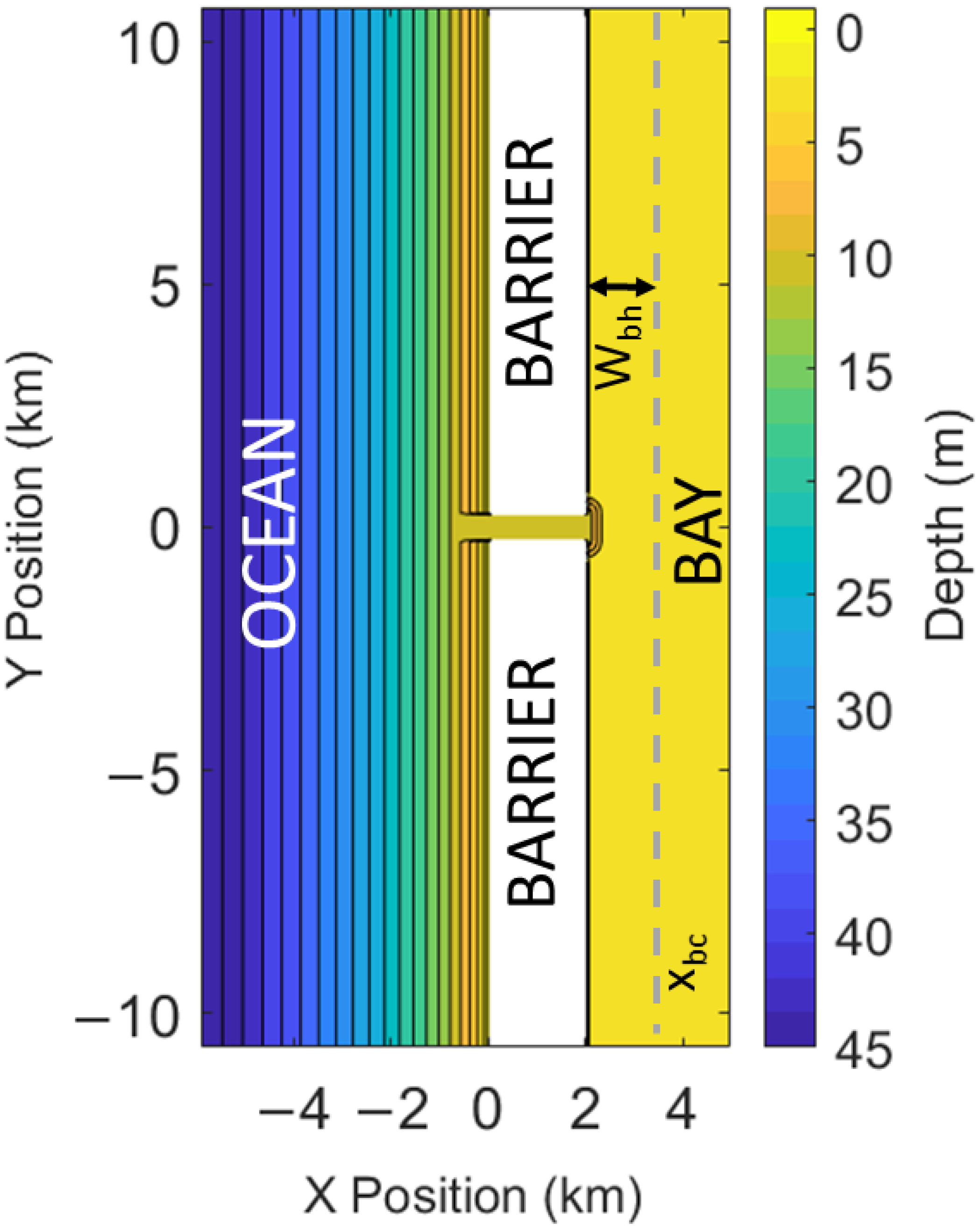
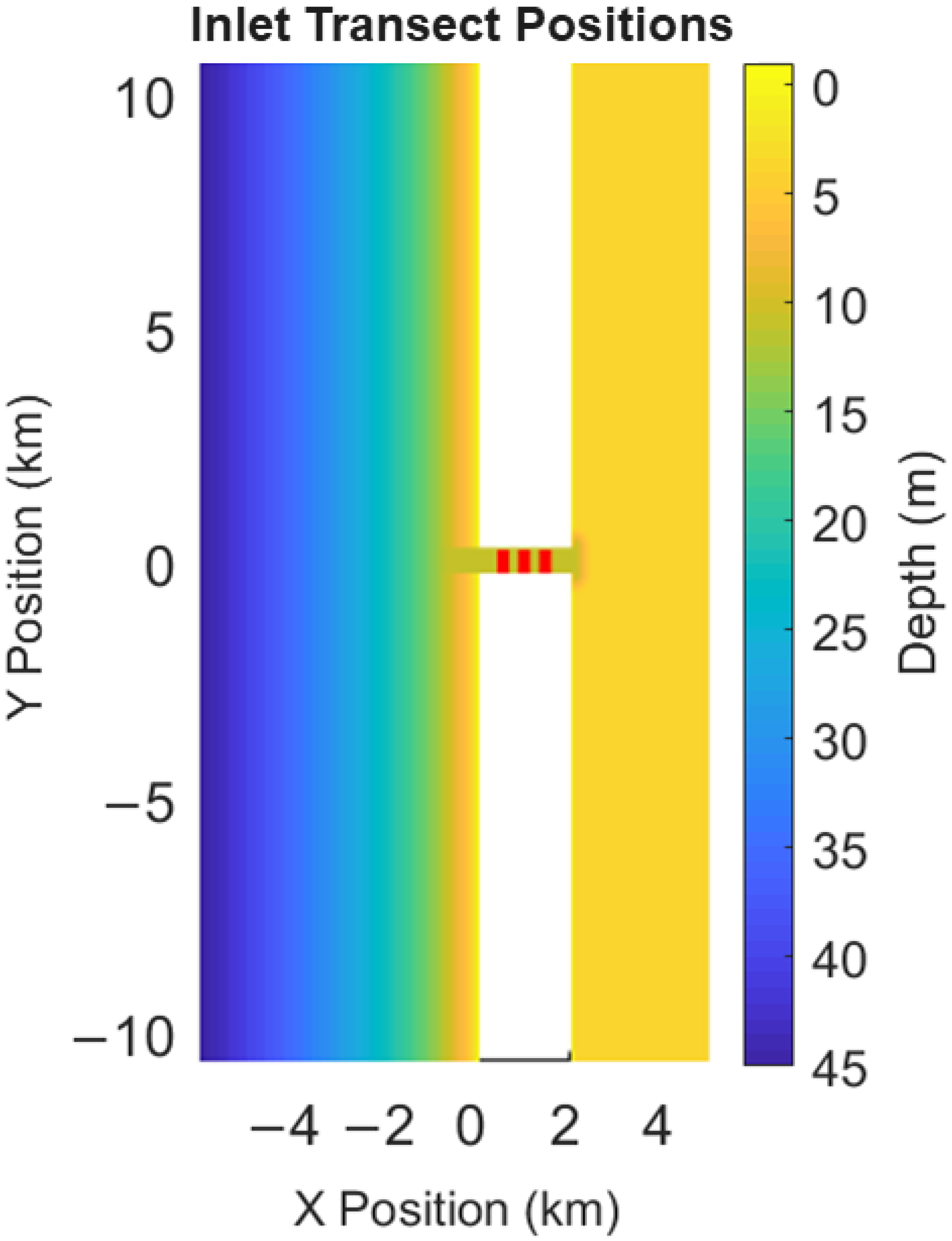
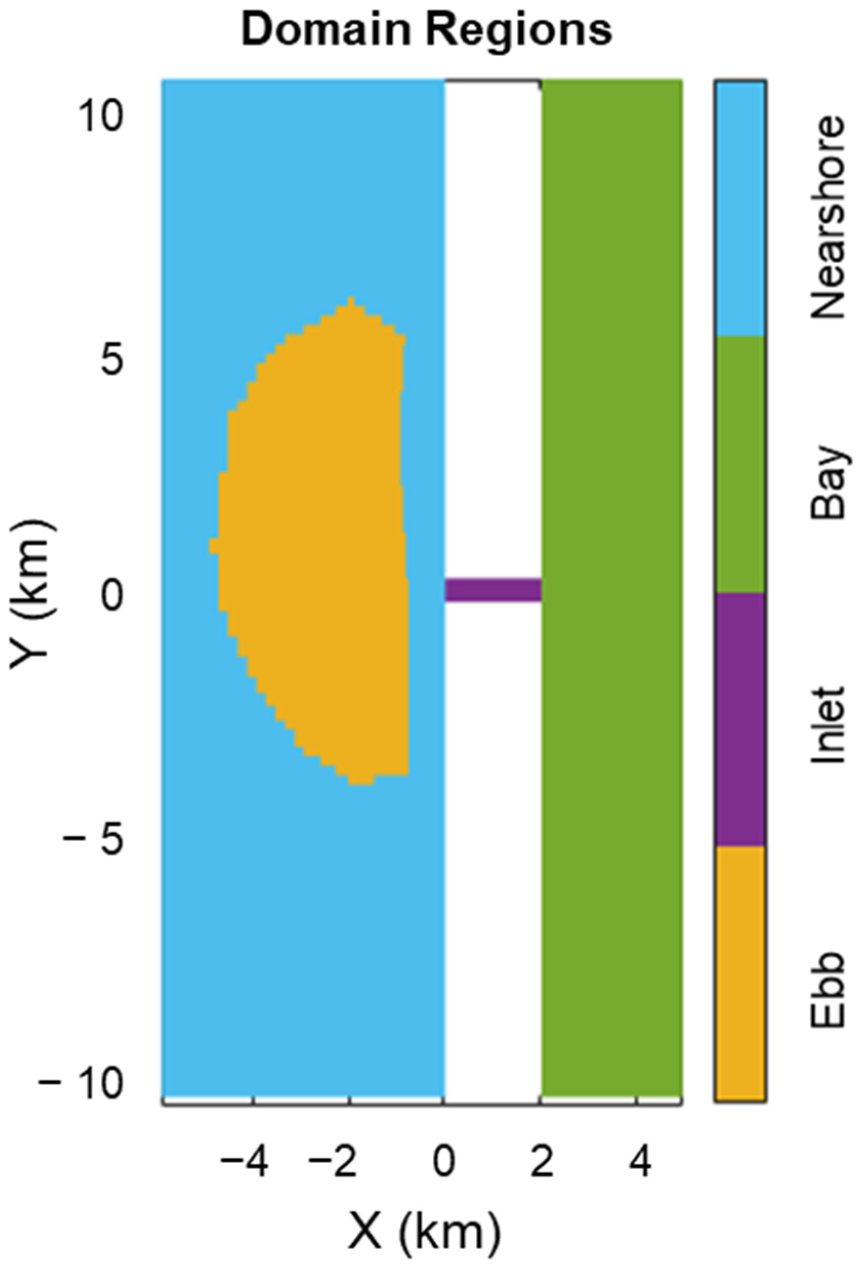
2.1. CMS Domain

Simulated domains and starting bathymetry were idealized based on the simplifications of the characteristics of the Humboldt Inlet following Styles et al. [19]. While the domain characteristics were defined to be representative of Humboldt Inlet, these features were idealized to permit comparisons across a broader range of bay systems, particularly lagoonal type barrier island systems. The domain was simplified to a rectangular inlet, bay, and nearshore oriented with the alongshore and along-bay axes on the Y-axis and the ocean on the left side of the domain. The along-inlet axis was oriented on the X-axis. Inlet and bay geometry was selected by matching the approximate horizontal aspect ratio and area of the real Humboldt Inlet system. The inlet dimensions were selected as approximately 2000 m by 550 m (Figure 1). The initial depth in the inlet was set as a constant value of 11.9 m, representing the average of considered bathymetry within the real inlet. While the real-world Humboldt Inlet is jettied, this characteristic was only partially represented in the numerical model domain. Cells along the sides of the inlet are defined as non-erodible, capturing the shore protection and inlet stabilization function of the jetties. The idealized nature of the approach and relatively coarse resolution was determined to make the jetty impact on ebb flow dynamics and littoral drift inadequately resolved. The bay dimensions were selected as approximately 22 km by 3 km (Figure 1). A reference depth of 3.4 m in the bay was determined from the average of considered bathymetry. Depths in the bay were varied to represent sediment distribution and availability and are described in Section 2.2. The offshore extent of the domain was established following Styles et al. [19] with the intention of minimizing the interaction between the ebb shoal and the offshore boundary. The dimensions of the ocean section of the domain were selected as 6 km by 22 km (Figure 1). Bathymetry outside of the bay and inlet were specified by an equilibrium beach profile [20], using the same profile as Styles et al. [19] (Figure 1). A single grain size of 0.20 mm was selected to match the sediment in the real inlet, following Styles et al. [19]. Sediment transport was calculated using the van Rijn [21] transport algorithm for non-cohesive sediments. A common model domain was applied in both CMS Flow and CMS Wave. The model domain was composed of 18,396 active cells, ranging from 50 m by 50 m in the inlet to 200 m by 200 m at the offshore edge. The X-coordinate grid refinement continued throughout the bay at the same cell spacing.

2.2. Initial Bay Bathymetry

Bay bathymetry was varied between simulations to represent the morphologic response to different hypsometric curves. Initial bathymetry within the bay was specified to be along-bay (Y, Figure 1) uniform and symmetric about the bay centerline (X_bc, Figure 1). A variety of starting bathymetries was analyzed to investigate the impact of sediment distribution within the bay on morphodynamic patterns.

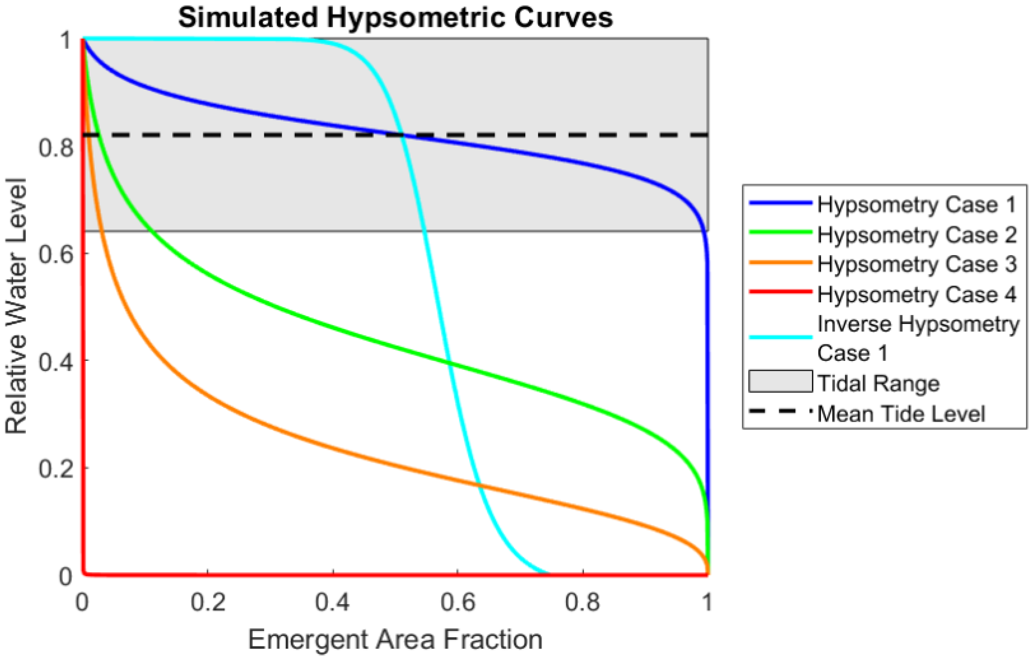
2.2.1. Systematically Varying Hypsometric Curves between Cases

In each case, bay depths were specified to fit a curve defined by the hypsometric curve equation presented in Strahler [6]:

$$y={\left(\frac{r}{1-r}\right)}^z{\left(\frac{1}{\left(1-r\right)R+r}-1\right)}^z$$

(1)

where:

• y = non-dimensional bed elevation that can range from 0 to 1;
• R = non-dimensional bay area that can range from 0 to 1;
• r = non-dimensional constant that can range from 0.01 to 0.5;
• z = non-dimensional constant exponent that can range from 0.03 to 2.

Bathymetry variations among cases altered bay storage volume and sediment availability. The selected hypsometric curves were determined as variations between a case with large inter-tidal areas and a case with no intertidal area. The extensively inter-tidal case was established with approximately half of the bay area submerged at mean tide. A hypsometric curve was selected by sampling viable parameter space and manually choosing between parameters which satisfy the half-submerged at mean tide condition. The bathymetry formed by the hypsometric curve defined as r = 0.02 and z = 0.05 was selected to represent a bay with a large inter-tidal area and is referred to as Hypsometry Case 1 (HC1, Figure 2).

Additional starting bathymetries were selected as variations between HC1 and a uniform bathymetry (HC4; r = 10⁻⁵, z = 0.99999; Figure 2). Two intermediate cases were established as Hypsometry Case 2 (HC2; r = 0.0167, z = 0.2083; Figure 2) and Hypsometry Case 3 (HC3; r = 0.0133, z = 0.3667; Figure 2). Areas above mean low water (MLW) and water storage vary over a wide range between HC1 and HC4 (Figure 2,

Table 1. Idealized Bay Morphology Characteristics: additional sediment relative to the uniform bathymetry case, percentage of the bay between MHW and MLW, volume of water in the bay between MHW and MLW, and the physical scenario represented in each case.

Case	Added Sediment (M m3)	Intertidal Area (%)	Intertidal Storage (M m3)	Represented Scenario
HC1	183	81	56	Large intertidal flats
HC2	98	8	95	Shallow sub-tidal areas
HC3	51	2	96	Deep sub-tidal areas
HC4	0	2	96	Featureless bathymetry
IHC1	135	48	54	Land reclamation

). An additional case was evaluated in which the inverse of the non-dimensional hypsometric curve defining HC1 was shifted to match the same condition of equal submerged and emergent areas at mean tide (IHC1, Figure 2).

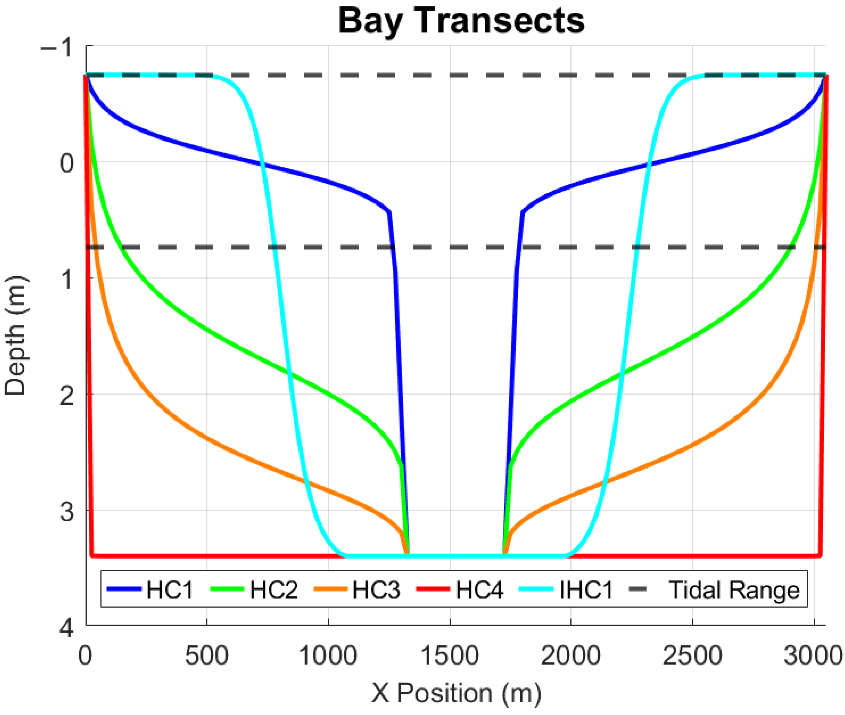
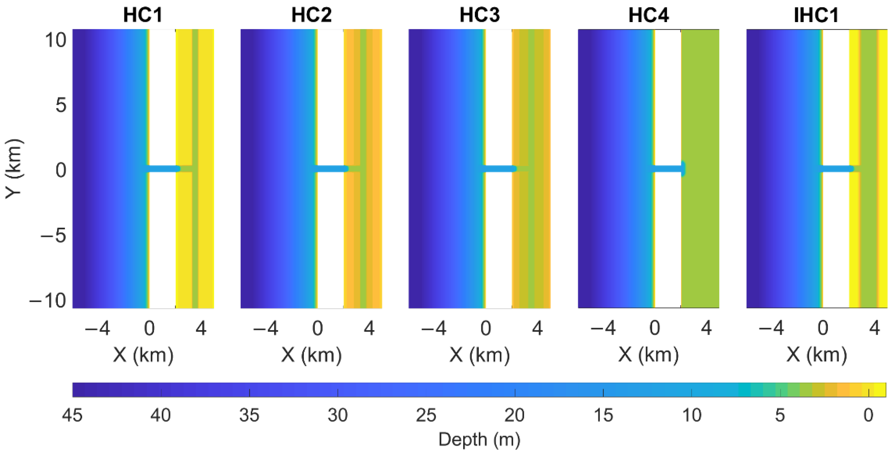
2.2.2. Developing Idealized Bathymetry from a Range of Hypsographs

The selected hypsometric curves were made dimensional with the bay half-width (W_bh, Figure 1) and reflected across the bay centerline (X_bc, Figure 1). An along-bay channel was added to the domain to maintain simulation stability (Figure 3). Maximum bay depths were constant in all starting bathymetries. Several changes were determined to be necessary to maintain simulation stability. The width of the channel along the center of the bay was iteratively increased for simulation stability. The width of the along-bay channel was set to 400 m because simulations with along-bay channel widths of 200 m became unstable. A limiting of the slope of 1:20 was also imposed on the across-bay elevation profile to minimize avalanching and resolve issues with the release of water trapped in inter-tidal areas. A wetting/drying depth of 0.2 m was also established to resolve further issues with the release of water trapped in inter-tidal areas. Modified initial bathymetries (Figure 3 and Figure 4) are expected to address the questions that guided initial hypsometric curve selection, but are not described by the same curves.

Each case represents a different basin configuration between extensive intertidal flats and a relatively deep uniform, featureless bathymetry (Figure 4). HC1 has extensive intertidal flats around a central channel, HC2 has many shallow subtidal areas, HC3 is relatively deep, HC4 is relatively deep and featureless, and IHC1 has many intertidal areas that are relatively high in the tidal frame. HC1 and IHC1 begin with similar intertidal storage volumes, but an additional 33% of the bay is intertidal in HC1 and an additional 48 M m³ of sediment begins the simulation in the bay (Table 1). HC2, HC3, and HC4 all begin with little to no intertidal area, resulting in similar intertidal storage volumes, but HC2 begins with 47 M m³ more sediment than HC3 and 98 M m³ more sediment than HC4 (Table 1). The differences between HC1, HC2, HC3, and HC4 represent a transition from large features, many of which are intertidal, to no features. Sediment availability and features on which sediment can deposit on or erode from were captured in the range of simulations. IHC1 has several similarities to HC1, but while HC1 represents large-scale wetland reclamation with areas at a large range of intertidal elevations, IHC1 instead represents land reclamation in which all intertidal area is high in the tidal frame.

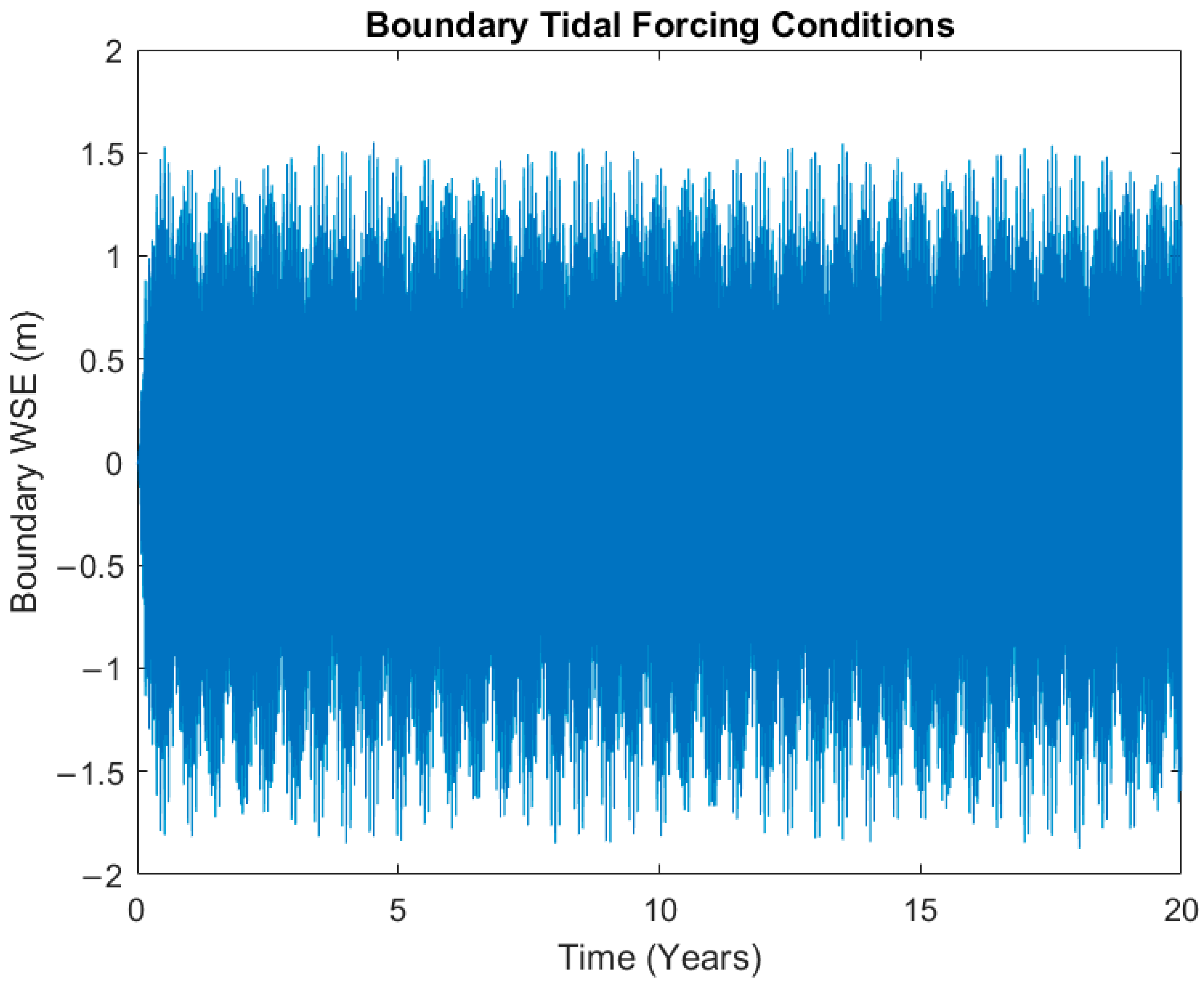
2.3. Tidal Forcing

The ocean boundaries of the domain were forced with 13 tidal constituents from Humboldt (

Table 2. Boundary forcing tidal constituents for North Spit, Humboldt Bay, CA.

Tidal Constituent	Amplitude (m)	Phase (Deg)
M2	0.7	215.1
S2	0.175	236.6
N2	0.148	190.5
K1	0.401	233.4
M4	0.012	200.6
O1	0.249	217.2
P1	0.126	231.3
SA	0.065	225.2
K2	0.047	228.3
Q1	0.044	211.3
SSA	0.038	264.1
NU2	0.029	194.5
L2	0.016	225.2

) to match Styles et al. [19]. Tidal constituent amplitude and phase were extracted from the National Oceanic and Atmospheric Administration (NOAA) tide database [22]. Mean tidal range was 1.49 m, with predominantly semi-diurnal components (primarily M2, S2 and N2), but large diurnal (primarily K1, O1, and P1) components as well. The thirteen selected constituents did not capture all tidal variation over the 20 years of tidal forcing at the physical site, but differences were considered to have a smaller impact than most of the simplifying assumptions. Selected tidal constituents capture multi-year tidal range modulations, with maximum boundary condition water levels of approximately 1.5 m (Figure 5).

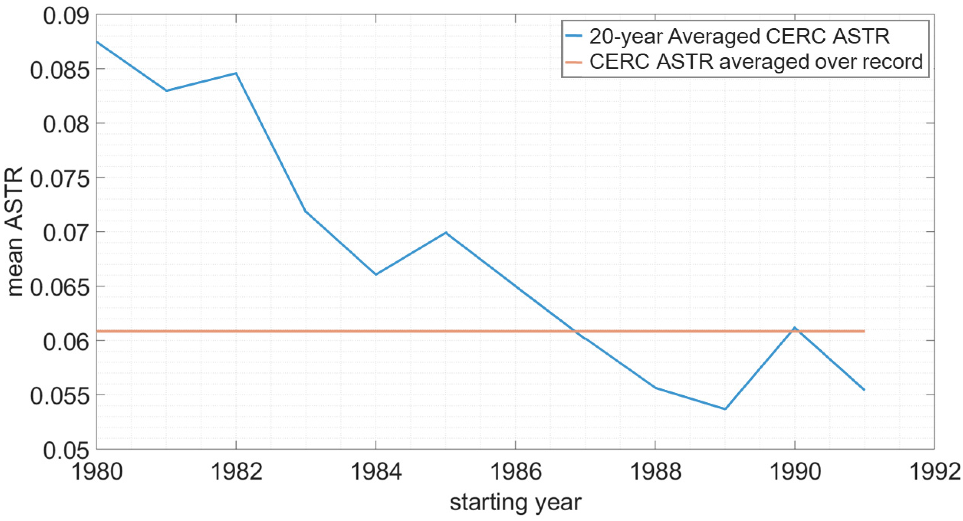
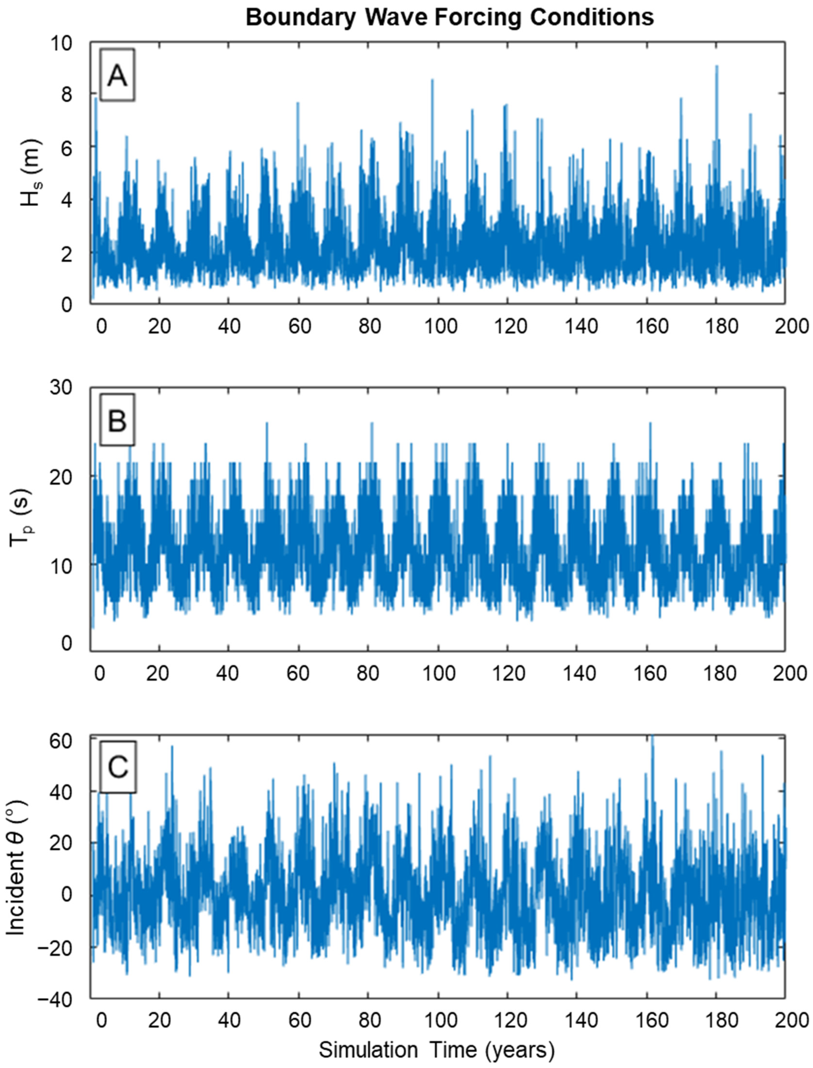
2.4. Wave Record Selection

A representative span of 20 years was selected from WIS station 83,047 to force the long-term inlet model simulation of a simplified representation of Humboldt Bay. Wave spectra characteristics (i.e., significant wave height (H_s), peak period (T_p), and mean wave angle (θ) were determined from the WIS station at a depth of 260 m. The offshore vector was estimated as 298° clockwise from north. The 20-year span with mean alongshore sediment transport rate closest to the mean over the entire duration was selected to represent a characteristic 20-year period. Alongshore sediment transport rate was estimated with the Coastal Engineering Research Center (CERC) formula as:

$$\mathrm{Q}=k\left(\frac{\rho \sqrt{g}}{16\sqrt{\gamma }\left({\rho }_s-\rho \right)\left(1-p_m^{\prime }\right)}\right)H_{br}^{2.5}\sin \left(2{\theta }_{br}\right)$$

(2)

where Q is the alongshore sediment transport rate in cubic meters per second, k is a constant (0.39), γ is the breaker index (0.78), H_br is breaking wave height, and θ_br is the breaking wave angle following Rosati et al. [23]. Wave height and angle at breaking were determined by iteratively shoaling the wave with Snell’s law and conservation of energy (in a method similar to the description provided by Dean and Dalrymple [20]) until the depth limited breaking criterion is met. The selected depth limited breaking criterion is described by:

$$H_{br}=\gamma ·h_{br}$$

(3)

where h_br is the depth at breaking. Wave spectra were transformed from the WIS station to depth limited breaking, following a similar procedure to Styles et al. [19]. Wave estimates at breaking were used to calculate CERC alongshore sediment transport rates over the entire record. The CERC alongshore sediment transport rate (ASTR) estimates were sampled with overlapping 20-year averaging windows and one year step size, and distributions of mean alongshore sediment transport estimates and mean alongshore sediment transport magnitude estimates were determined (Figure 6). The 20-year span with the most representative mean alongshore sediment transport rate estimate was determined to begin on 1 January 1990. Selected significant wave heights varied from 0.205 to 9.08 m with a mean of 2.15 m, selected peak periods varied from 2.64 to 26.0 s with a mean of 11.2 s, and selected incident wave angles varied from –32.7° to 61.6° with an energy weighted mean of 1.14° (Figure 7).

2.5. Analysis Techniques

Model output from simulations was analyzed with a variety of techniques to compare morphodynamic and hydrodynamic differences associated with the range of the considered starting bathymetries and the factors related to net sediment transport to or from the bay.

2.5.1. Morphology and Elevation Data

Morphology was output from the model at intervals of 20 effective days of forcing. This higher frequency data facilitates temporal comparisons, but spatial patterns are only presented as starting and ending conditions to limit extraneous content. Morphology and intertidal area patterns are described in Section 3.1 to present the full model results that are used to quantify the various differences among the cases in the subsequent sections. Elevation and bathymetry data in the bay are binned into hypsographs in Section 3.4 to characterize the basic information about changes in elevation distributions among the different cases. Morphology change was calculated by subtracting the morphology at a specific time-step from the initial morphology. This is interpreted as net sediment transport and is integrated over specific regions of the domain in Section 3.2 to describe sediment and large-scale import and export. The combined morphology information indicates the most important differences among the cases that gain or lose sediment from the bay.

2.5.2. Tidal Asymmetry

Tidal asymmetry was addressed through analysis of the peak velocities and the duration of the flood and ebb cycles in the inlet. The impact of bathymetry on tidal asymmetry was investigated through one-year simulations without wave forcing or sediment transport. Tidal asymmetry associated with bathymetry from 0, 25, 50, 100, and 200 years of simulated morphologic change was investigated for each case, for a total of 25 additional simulations. Water elevation and velocity data were output at 300 s at each point along defined transects in the inlet to improve temporal resolution of tidal signals (Figure 8).

A weighted average was applied to along-channel velocity data from the three central transects across the inlet to normalize by water volume. Peak velocities were determined for each ebb and flood cycle from the spatially averaged inlet velocities and compared to evaluate peak velocity asymmetry. Peak velocity asymmetry is presented as the average of the difference between these peak flood and ebb velocities over the year of simulated tidal forcing divided by the average of the non-dominant peak velocities. The durations of ebb and flood cycles were also determined from spatially averaged inlet velocities, with positive velocities corresponding to flood tide and negative velocities corresponding to ebb tide. Ebb and flood durations were compared to evaluate tidal duration asymmetry and are presented as relative differences. Tidal duration asymmetry was calculated as the difference between flood and ebb tide durations divided by the duration of the non-dominant tide (i.e., ebb tide for flood dominant asymmetries and vice versa). Tidal asymmetry informs the interpretation of the morphologic results, as results can generally be grouped between flood- and ebb-dominant asymmetry in the inlet.

3. Results

3.1. Morpho-Sedimentary Evolution

Morphology results indicate that the impact of hypsometry on bay morphology change varies between regions of the domain. Differences are particularly evident in the ebb shoal and channel patterns in the bay. These impacts were assessed by comparing bathymetry to morphologic changes after 200 years.

Morphology changes in several similar ways in all five simulations, indicating the tested range of initial bathymetries only had minor impacts in several regions of the domain. In all cases, the inlet deepens, and relatively deep channels develop through much of the bay. Inlet morphology does vary between simulations, but all cases developed a deep channel along the northern side of the inlet (Y > 0) and a shoal along the southern side (Y < 0). A large, more than 100 M m³ ebb shoal also forms a small distance offshore of the inlet in all simulations. Ebb shoal volume is compared to volumes of sediment transported to or from other regions of the domain (see Section 3.2), but specific ebb shoal morphology patterns are not presented in detail. The model also predicts the extensive flattening of the shallower nearshore area within approximately 500 m of the ocean-side shoreline for all tested simulations. Nearshore erosion in tested simulations is not expected to match natural systems, but likely results from limitations in the model setup and the long duration.

Simulations do predict important differences between initial bathymetry configurations in other regions of the domain. Flood dominant cases (HC2, HC3, and HC4) build extensive flood shoals and deposit sediment in intertidal shoals along the sides of the meandering channels that form in the bay (

Table 3. The initial and final added volume of sediment, intertidal area, and intertidal storage in the bay for each simulation.

Case	Added Sediment (M m3)		Intertidal Area (%)		Intertidal Storage (M m3)
	Initial	Final	Initial	Final	Initial	Final
HC1	183	118	81	62	56	71
HC2	98	81	8	17	95	91
HC3	51	67	2	16	96	90
HC4	0	22	2	9	96	93
IHC1	135	117	48	47	54	58

). Ebb dominant cases (HC1 and IHC1) deposit some sediment across from the inlet (Y ≈ 0), but erode larger volumes of sediment from the intertidal areas (Table 3). The bay loses more sediment in simulations where more sediment begins in the bay (Table 3), but differences on the order of tens of millions of cubic meters remain in the final volumes of sediment in the bay.

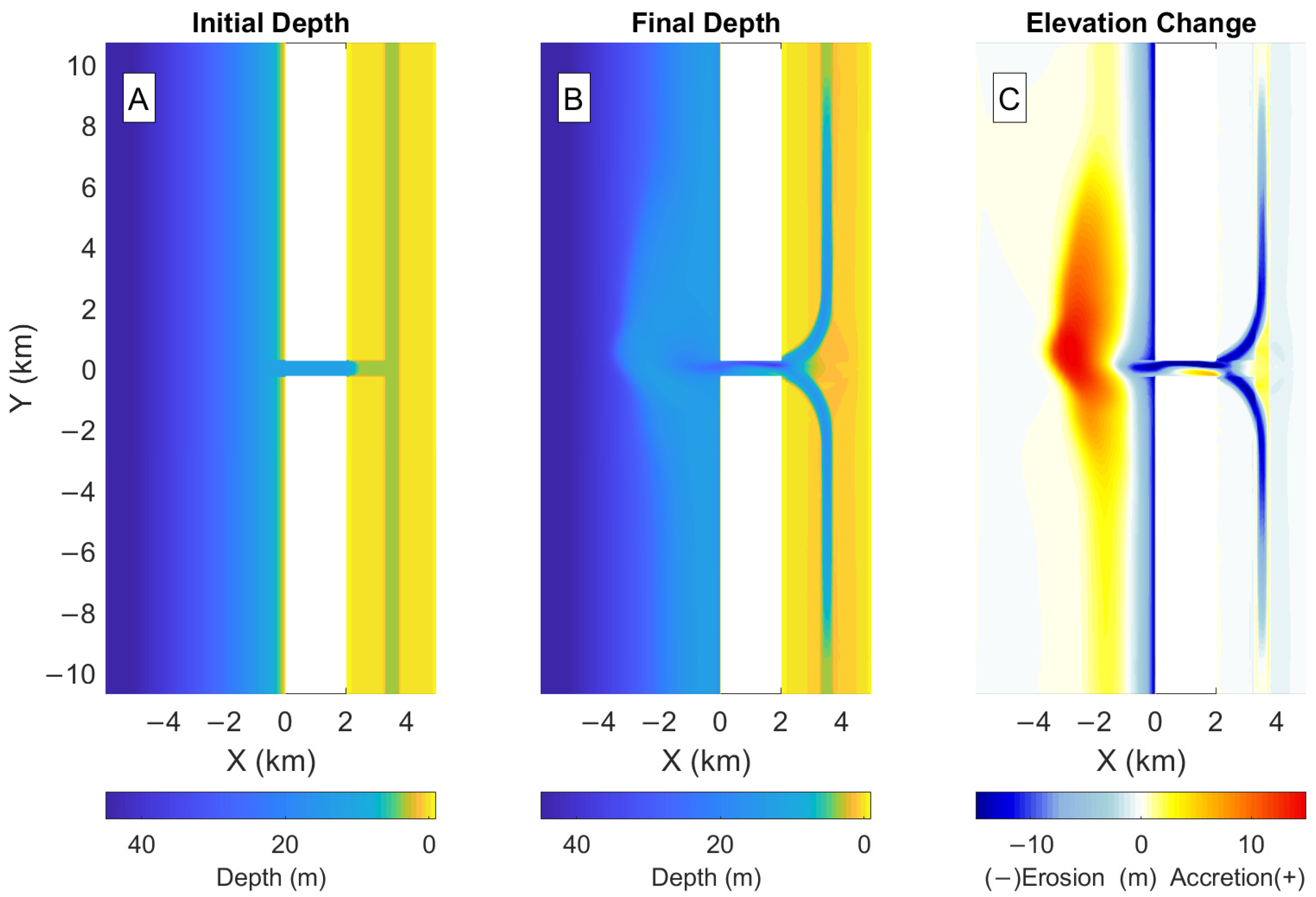
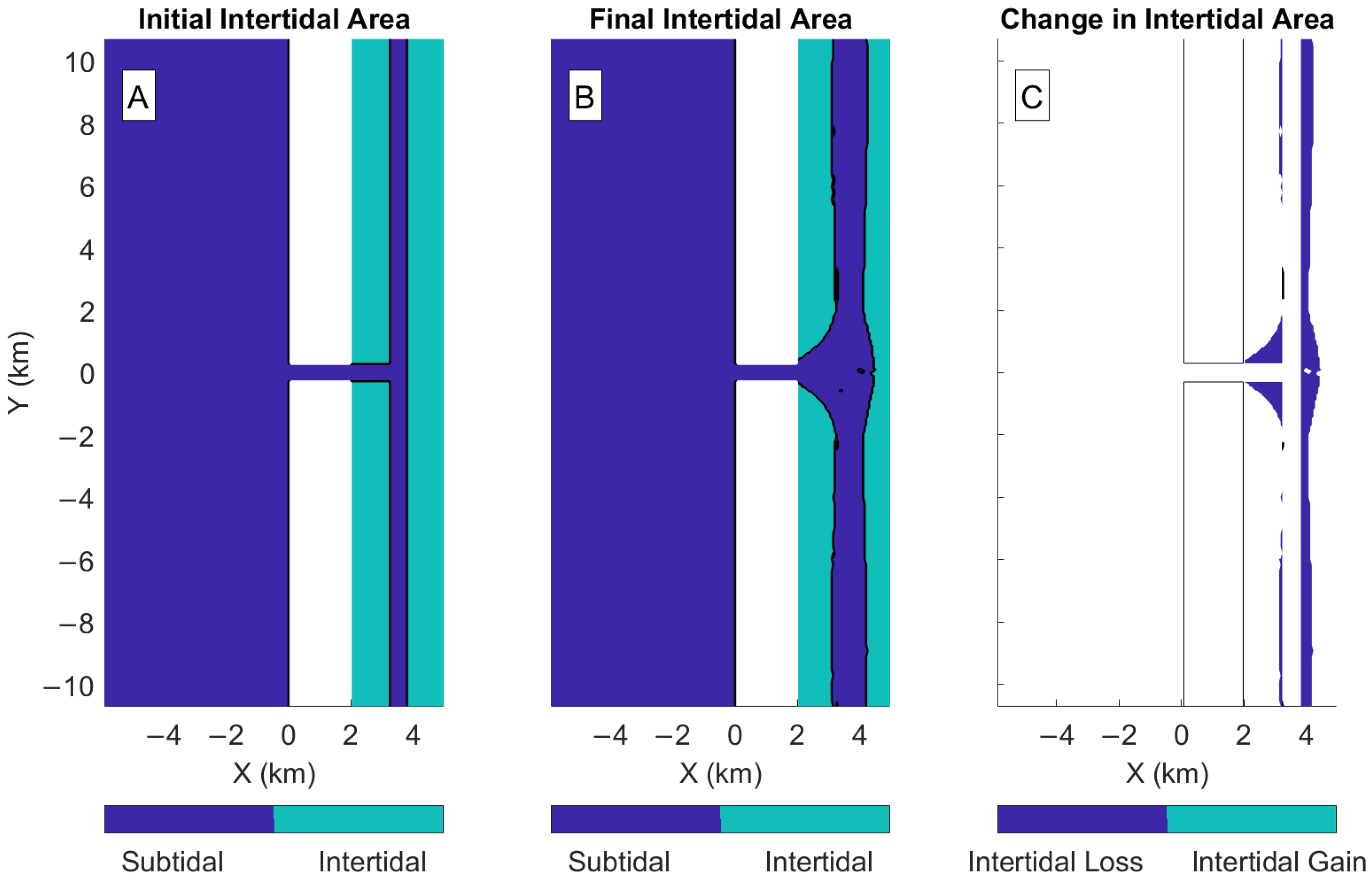
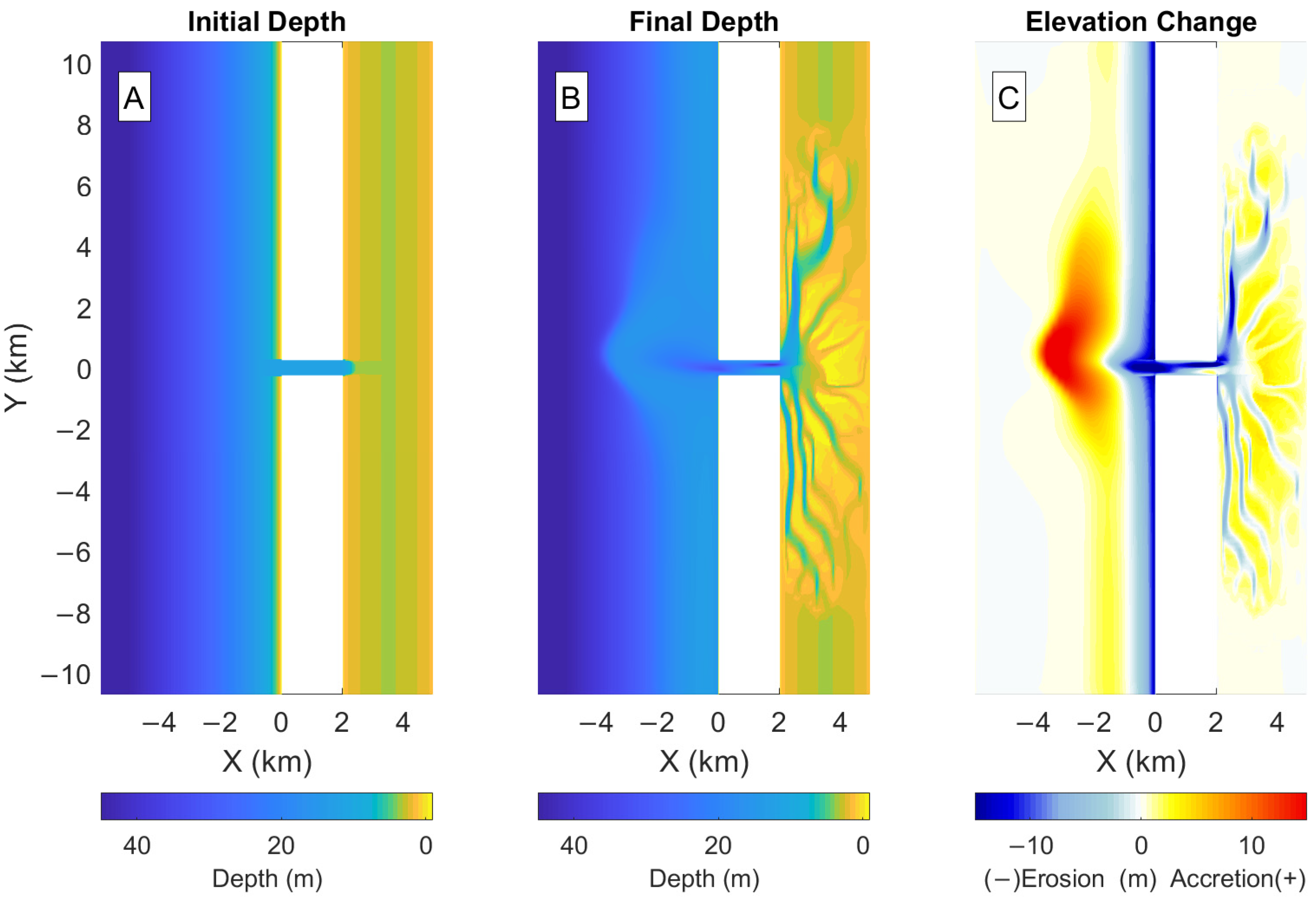
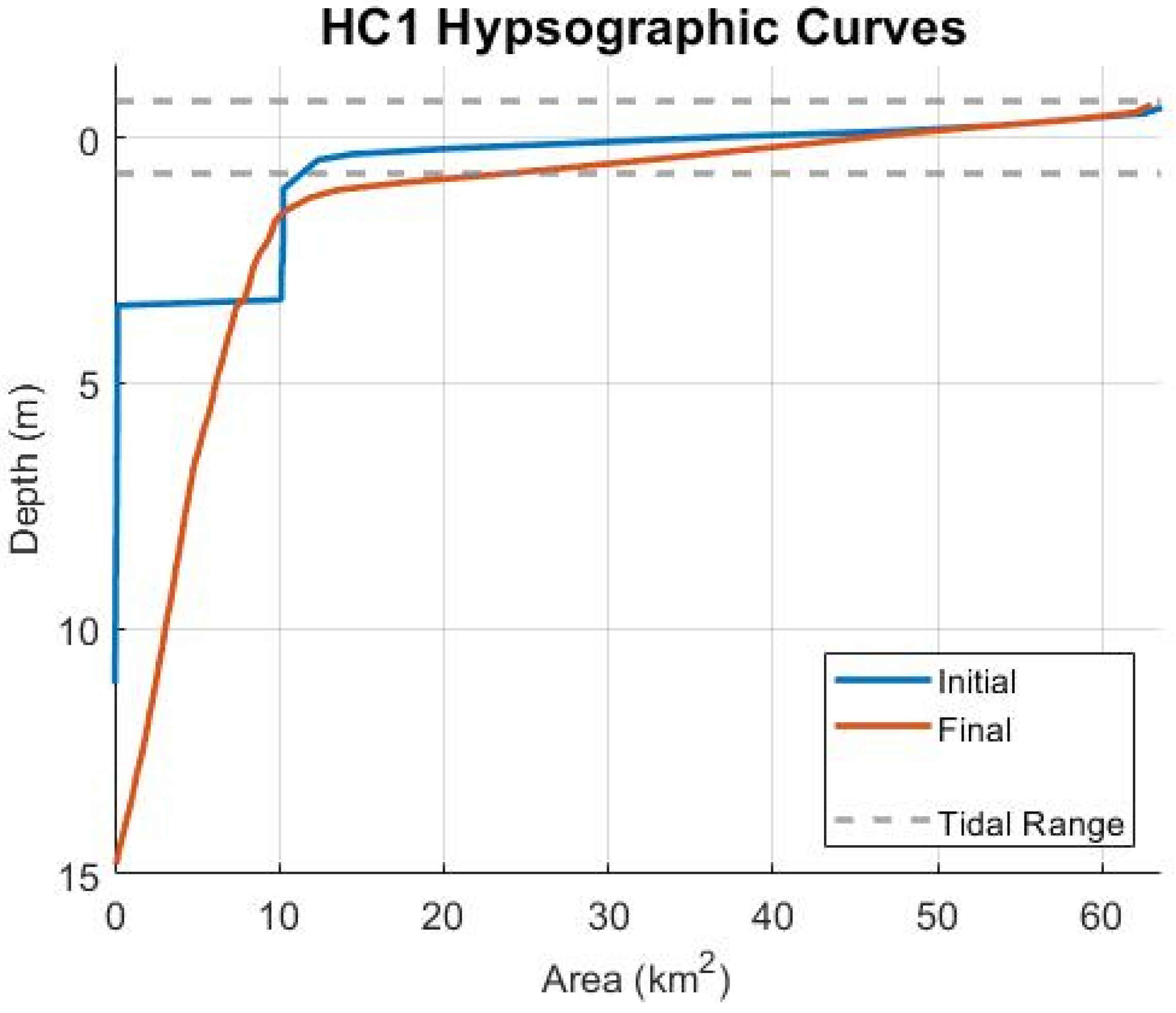
3.1.1. HC1 Morphology

In HC1, morphology change in the bay is dominated by the initial channel deepening (Figure 9). The channel connecting the inlet to the along-bay channel also carves through the inter-tidal area near the inlet to shorten the flow path. Accretion is predominantly in an ebb shoal, but some accretion also occurs in flood shoal landward of the inlet. The intertidal area decreases from 81% of the bay to 62% throughout the simulation, with the greatest intertidal area loss near the inlet and adjacent to the along-bay channel (Table 3, Figure 10). The morphologic evolution in HC1 simulates the continued prevalence of the singular deep channel, as the channel erodes and intertidal area reduces. The realism of this singular streamlined channel is difficult to assess. Other idealized numerical modeling has suggested that several of the common techniques for incorporating of bed slope effects can adversely impact long time-scale channel behavior predictions specifically leading to over-incision and a lack of branching (e.g., [24]).

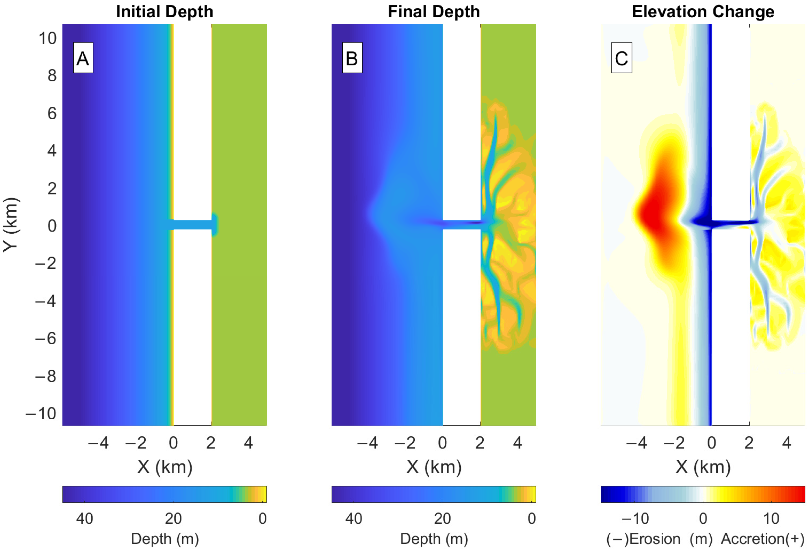
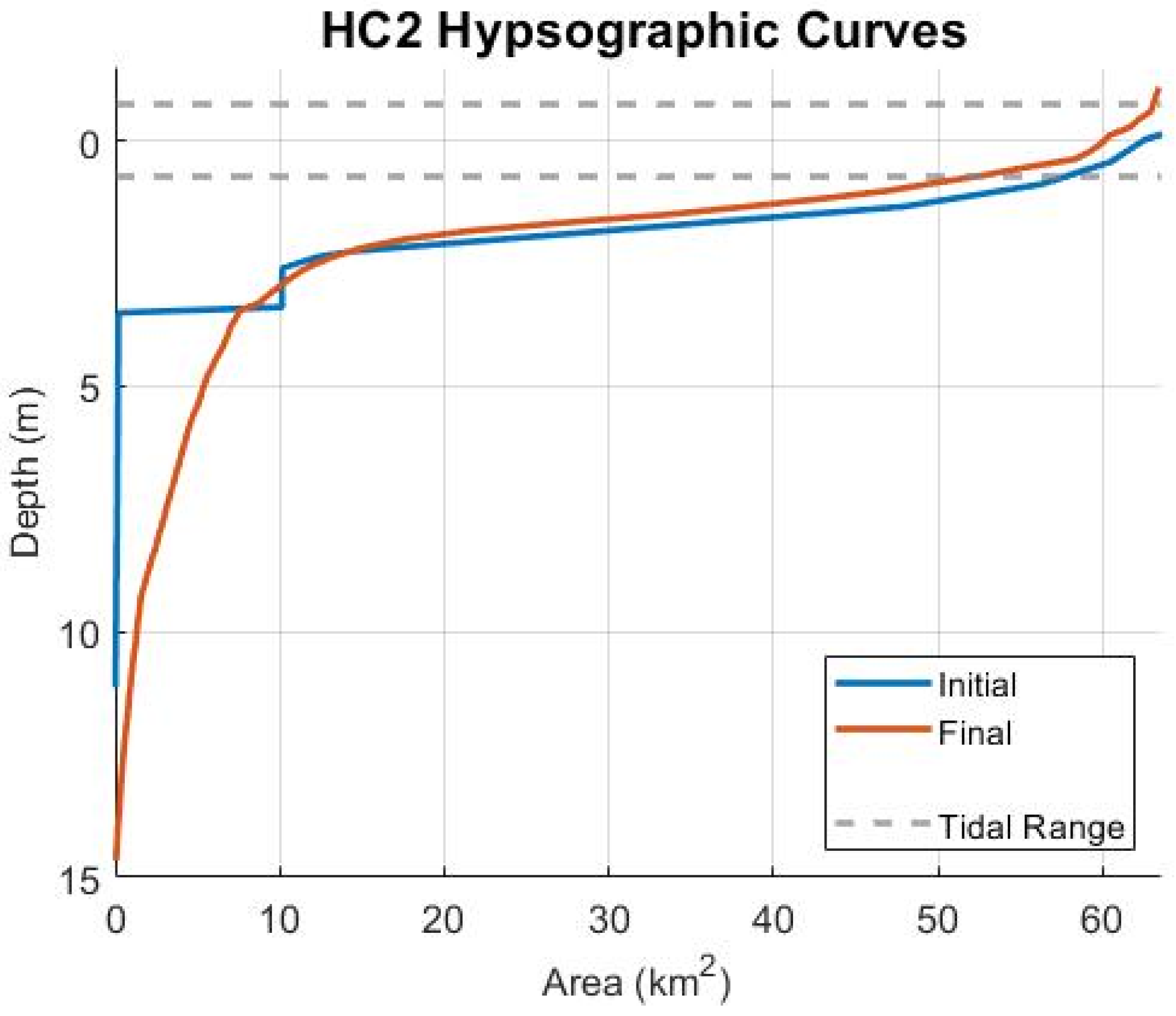
3.1.2. HC2 Morphology

In HC2, the shallow subtidal areas adjacent to the main channel along the bay and across from the inlet accumulate sediment (Figure 11). The central channel deepens and migrates towards the inlet. Several secondary channels also form off the primary along-bay channel. The intertidal area more than doubles through the course of the simulation with the formation of emergent shoals across from the inlet and on the edges of the channel along the bay (Figure 12). The 85 M m³ more sediment and 71.8% less of the bay beginning as intertidal area in HC2 are predicted to correspond to shallower, less streamlined channels and more shoal formation throughout the bay than in HC1 (Table 1, Figure 11). Many of the depositional features in the bay also become intertidal (Figure 11 and Figure 12). The net sediment flux between the bay and the other regions of the domain show that more sediment is eroded from the channels than is deposited in the shallow subtidal areas.

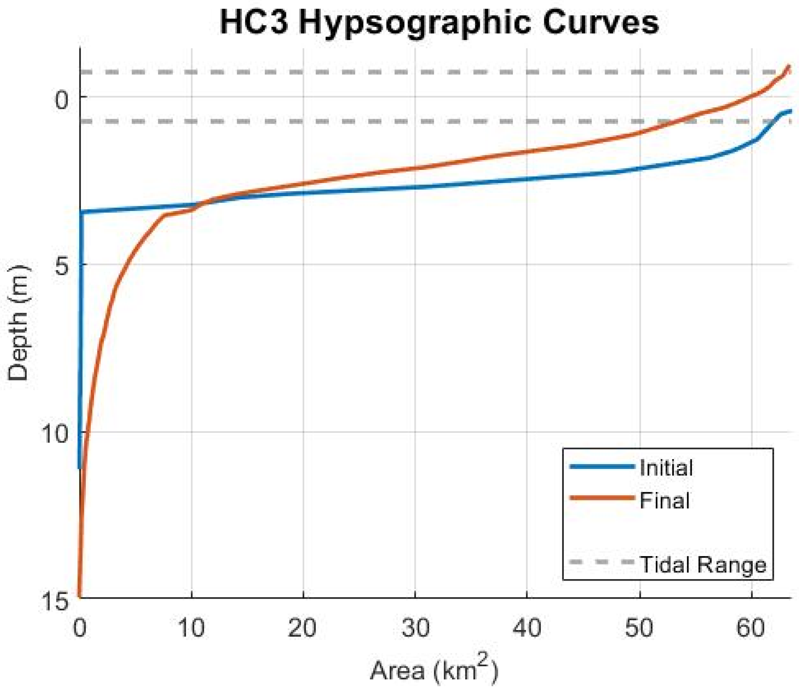
3.1.3. HC3 Morphology

In HC3, channels form and deepen through the relatively deep sub-tidal areas (Figure 13). These channels are shallower and more numerous than the channels of HC1 or HC2. Shoals form across from the inlet and along the channels. The pattern of channels and shoals in the bay is also less symmetric about the line X = 0. The intertidal area increases from 2% to 16% of the bay, as many of the shoals that form become intertidal (Figure 14). The deeper subtidal areas of HC3, corresponding to 47 M m³ less sediment beginning in the bay, contribute to 16 M m³ more sediment being imported into the bay than in HC2 (Table 3). Net sediment flux is transported into the bay, so more material is deposited in the shoals than is eroded from the channels.

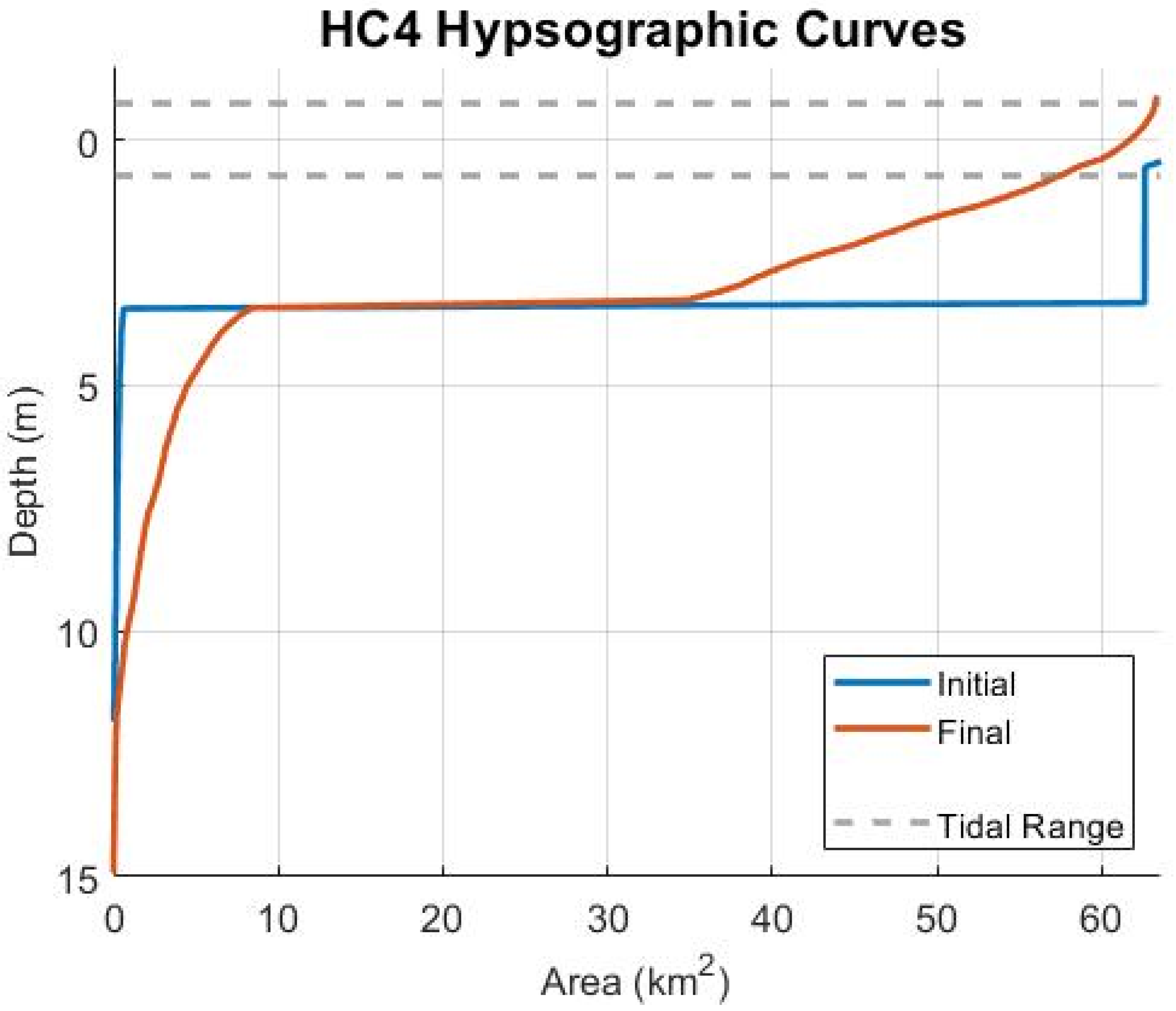
3.1.4. HC4 Morphology

In HC4, channels form and deepen through the initially featureless bay bathymetry (Figure 15). Channels in HC4 are wider and less numerous than in HC3 and shallower than the channels of HC1 or HC2. Shoals form across from the inlet and along the channels. Accretion occurs throughout the central two-thirds of the bay (Figure 15). The balance of shoal and channel formation result in the net import of 22 M m³ of sediment (Table 3). HC4 imports 6 M m³ more sediment than HC3, but the initially deeper bay results in 7% less of the bay being intertidal. The intertidal areas that do form are located between the wider channels (Figure 15 and Figure 16). These differences from HC3 are related to the additional 51 M m³ of sediment with which HC3 began in the relatively deep sub-tidal areas (Table 3). The morphologic evolution in HC4 simulates the formation of several channels through an initially featureless bay with relatively large intertidal shoals forming between channels (Figure 15).

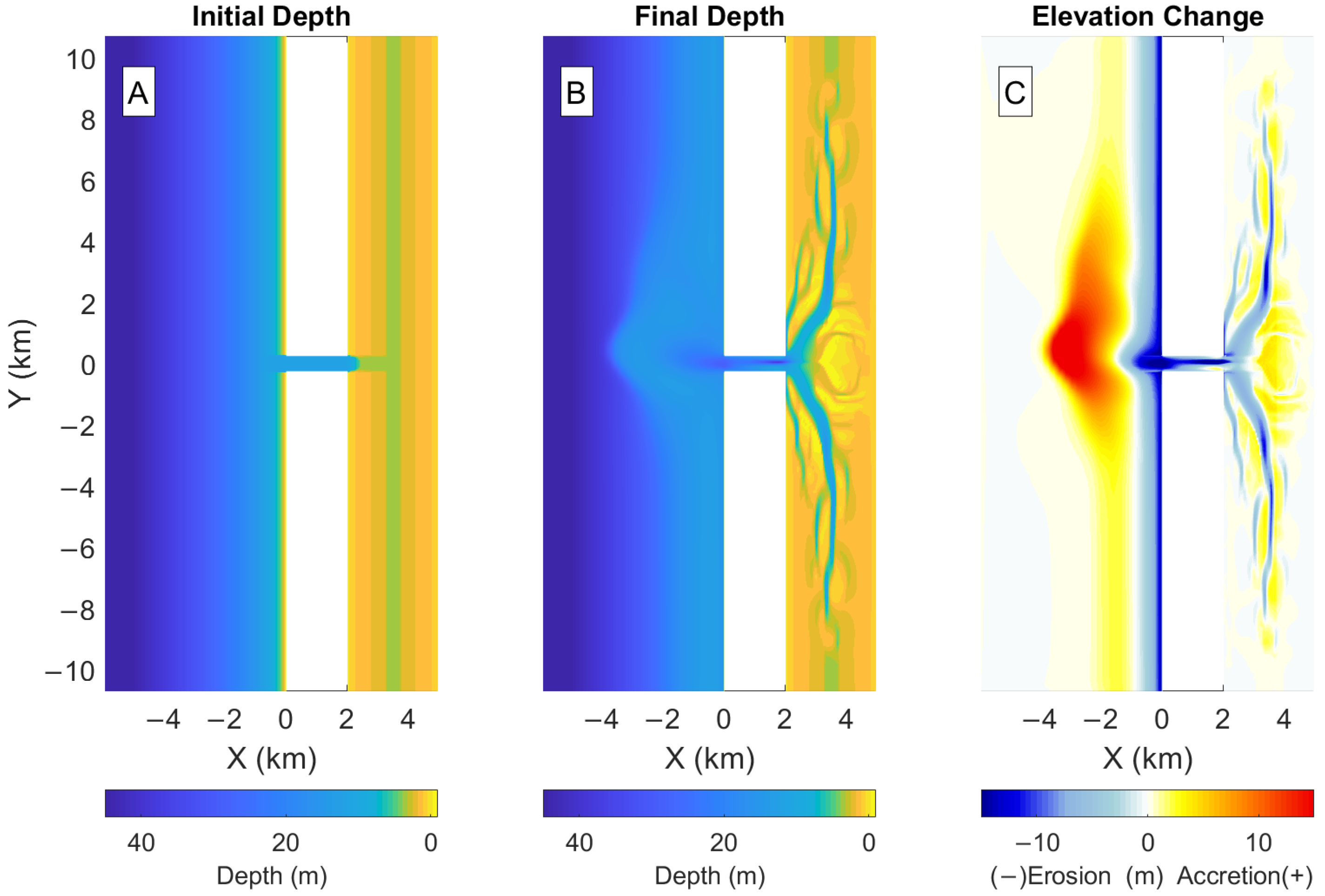
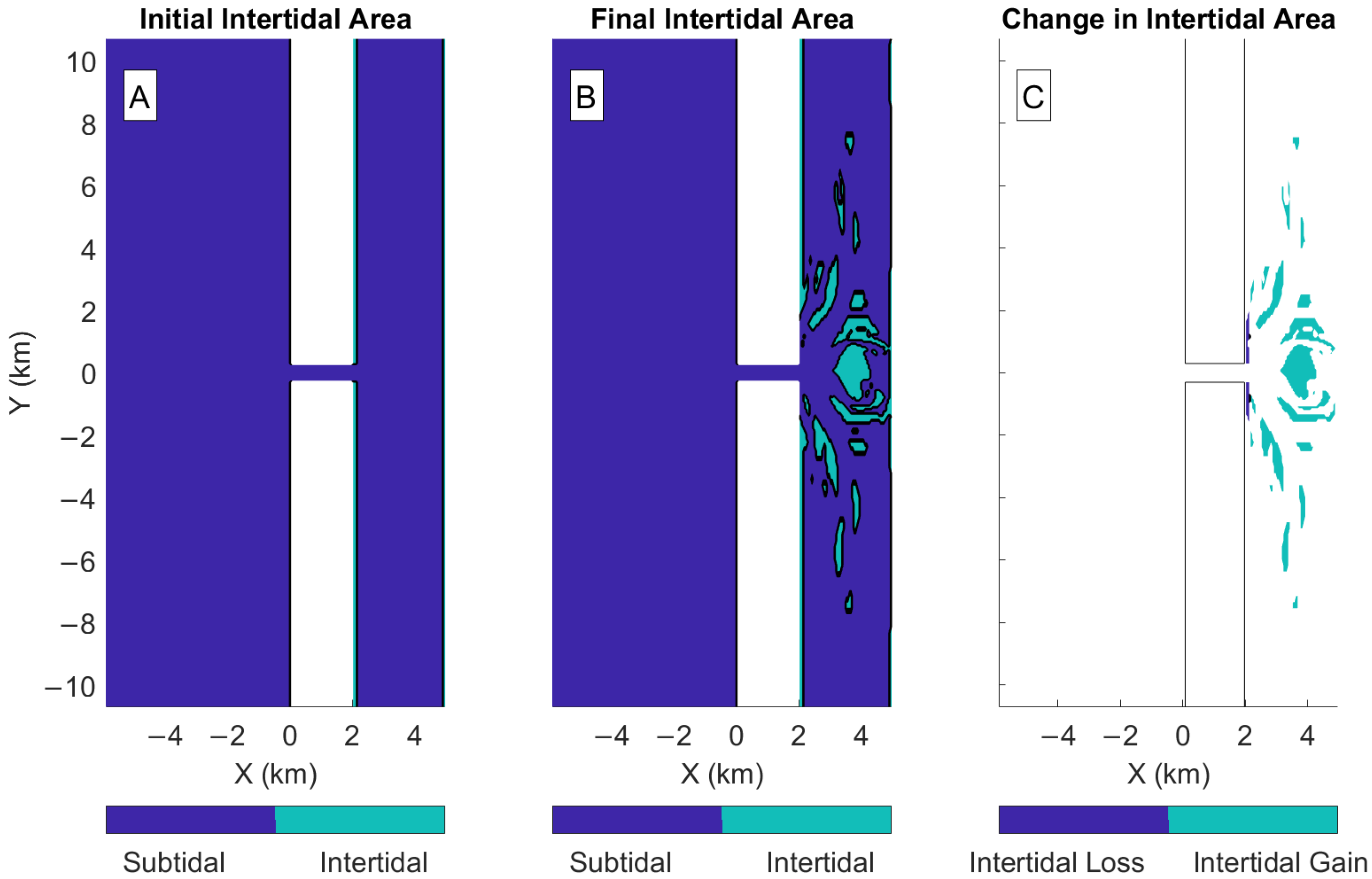
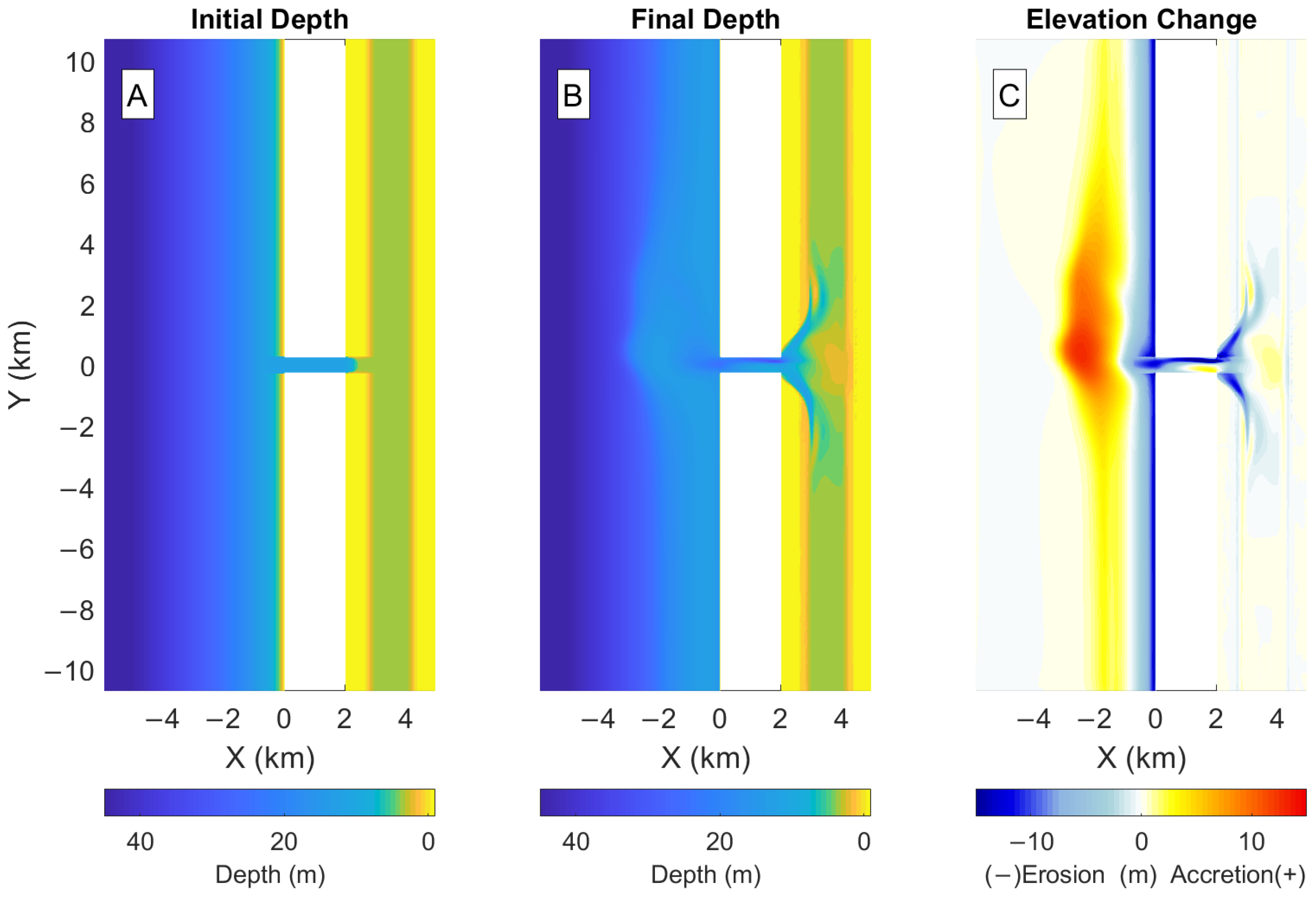
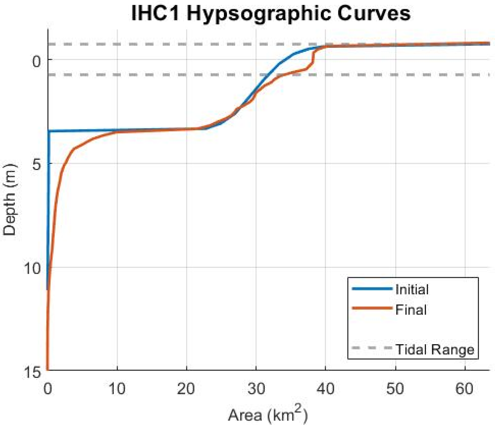
3.1.5. IHC1 Morphology

In IHC1, much of the morphology change in the bay is intertidal erosion, particularly within 1 km of the inlet (Figure 17). The intertidal area near the inlet decreases slightly, but the changes only represent 1% of the bay area (Figure 18). Material is removed from the intertidal areas in such a way that it is transported out of the bay and only has a minor impact on the fraction of the bay that is intertidal. While all other cases lose material from relatively extensive channels and channel networks, channel features in IHC1 do not extend more than 2 km from the inlet. Approximately 18 M m³ of sediment is exported from the bay, but the volume of sediment in the bay remains 36 M m³, 50 M m³, and 95 M m³ higher in IHC1 than in HC2, HC3, and HC4, respectively (Table 3). The morphologic evolution in IHC1 simulates the erosion of the edges of the elevated intertidal area, particularly near the inlet.

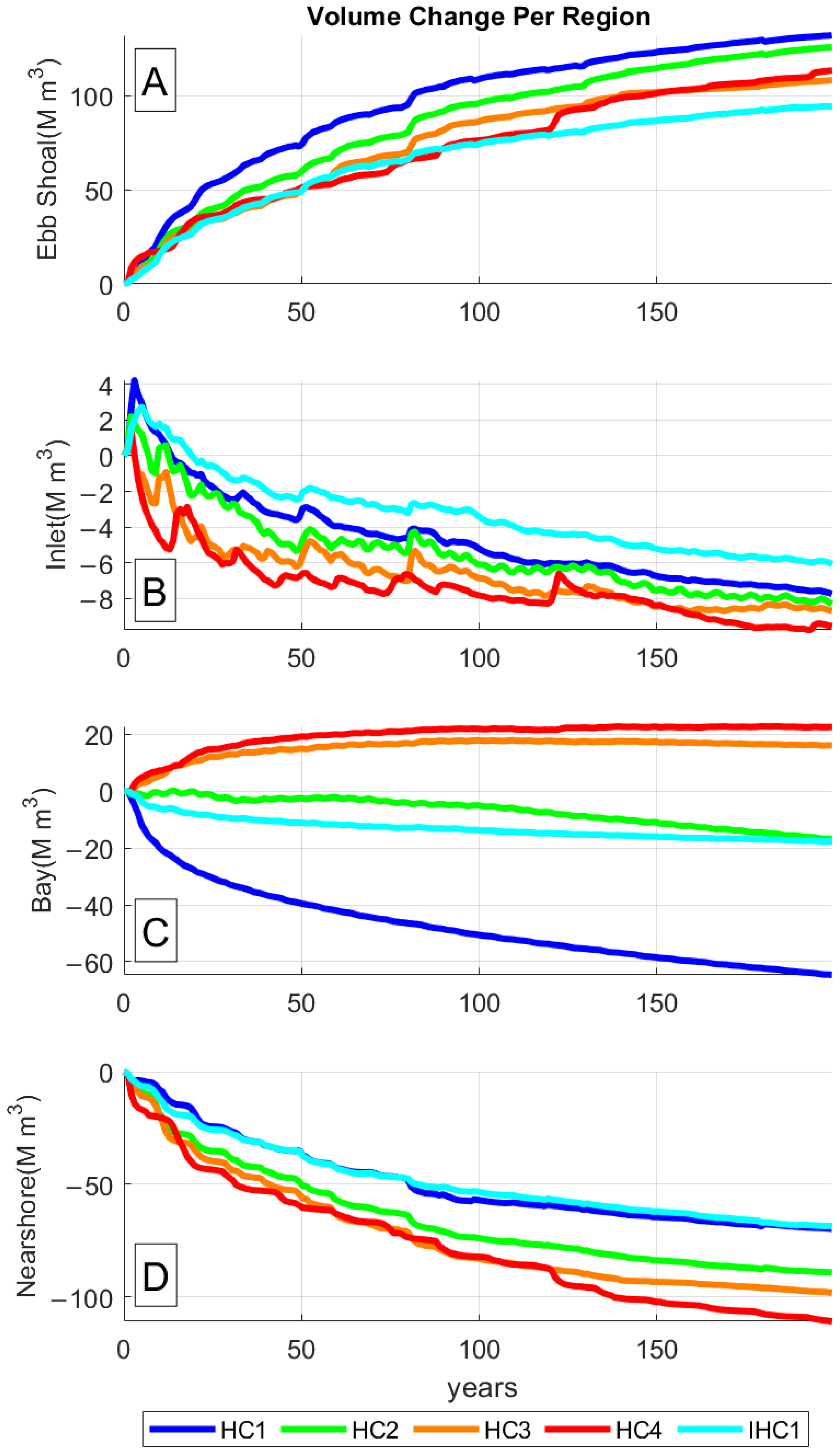
3.2. Morphodynamic Change by Region

The domain was divided into four regions to investigate sediment import and export trends in the ebb shoal, the inlet, the bay, and the nearshore (Figure 19). The inlet and bay have simple designations as the area between the two sides of the barrier and the area landward of the barrier, respectively. The area indicated as the ebb shoal was selected by hand as the extent of substantial accretion outside of the inlet with a manually selected buffer. The nearshore region was configured to exclude the area designated as the ebb shoal.

3.2.1. Net Sediment Transport between Regions of the Domain

Each simulation predicts the formation of a 150+ M m³ ebb shoal, the removal of 5–10 M m³ of sediment from the inlet, and the loss of 60–100+ M m³ of sediment from the nearshore (Figure 20). Specific volumes vary among cases, but magnitudes and signs are similar. The inlet loses sediment in all cases. The net volume of sediment predicted to leave the inlet appears to be related to tidal prism in these simulations. This aligns with a variety of studies that have found inlet cross-section to be related to tidal prism (i.e., [25,26,27,28]). After 200 years of morphology change, the tidal prisms of HC2, HC3, and HC4 are similar, HC1 has approximately three quarters of that magnitude, and IHC1 has approximately two thirds of the tidal prism in HC4 (Table 3). The volume of sediment that leaves the inlet follows a loosely similar pattern, with HC4 inlet losing the most sediment and the IHC1 inlet the least. All simulations also lose sediment from the nearshore. The transfer of sediment away from the nearshore is likely impacted by some of the limitations of the modeling approach but appears to have some connection to the volume of sediment being imported into or exported from the bay and the volume of ebb shoal.

Ebb shoals grow in all cases, but the volumes vary. Researchers have related ebb shoal volume to a variety of influences, but the volumes of several ebb shoals have been related to tidal prism with strong influences from the tide and wave energy regime, energy flux through the inlet [29], and the angle between the outflow jet and the shoreline [30]. Similarly, the closely related features that often form at the mouths of rivers (river mouth bars) have been found to be strongly influenced by outflow inertia (e.g., [31,32]). Differences between ebb shoal volume predictions do appear to be related to these characteristics, but they are not entirely described by these differences between cases. Ebb shoal volume in HC1, HC2, HC3, and HC4 also appears to be strongly related to volume imported into or exported from the bay, with the sediment supply from HC1 corresponding to a large ebb shoal and the sediment trapping of HC3 and HC4 corresponding to smaller ebb shoals. Large volumes of available sediment have been found to have a strong influence on ebb shoal volume and formation (e.g., [33,34,35]), which these model results also indicate. Differences in sediment availability do not appear to describe the different ebb shoal volume of IHC1. Although the bay loses a similar volume of sediment in HC2 and IHC1, the reduced tidal prism of IHC1 may contribute to the smaller ebb shoal volume, which is consistent with previous findings on the impact of the tidal prism on the ebb shoal volume (i.e., [29,30]).

Sediment import or export from the bay does vary among cases. The net volume of sediment entering and leaving the bay relates to the balance of channel formation and accretion or erosion elsewhere. The ebb dominant cases (HC1 and IHC1) both lose sediment from the bay, but HC1 exports more than twice as much sediment as IHC1 (Figure 20). This additional erosion corresponds to the longer channel through the bay and more widespread erosion. The bay does not gain sediment in all flood-dominant cases. The balance between channel formation and sediment deposition results in net export in HC2, but net import in HC3 and HC4.

In all cases, most regions gain or lose sediment at much faster rates in the first 10 to 25 years of the simulation. Sediment export from the bay in HC2 does not follow the same trend as the other cases. The volume of sediment in the bay remains relatively constant for the first 60 to 70 years and decreases through the rest of the simulation. This transition corresponds to the gradual shift from adding intertidal area to maintaining the same coverage of the bay (Figure 21). The rate of intertidal area addition also reduces to near zero over the course of HC3 and HC4, but these changes correspond to less of a change in the volume of sediment in the bay. Sediment export from the bay loosely corresponds to more sediment in the ebb shoal, inlet, and nearshore, but the distribution varies between simulations. The boundary conditions allow sediment to enter and exit the domain, so sediment is not conserved.

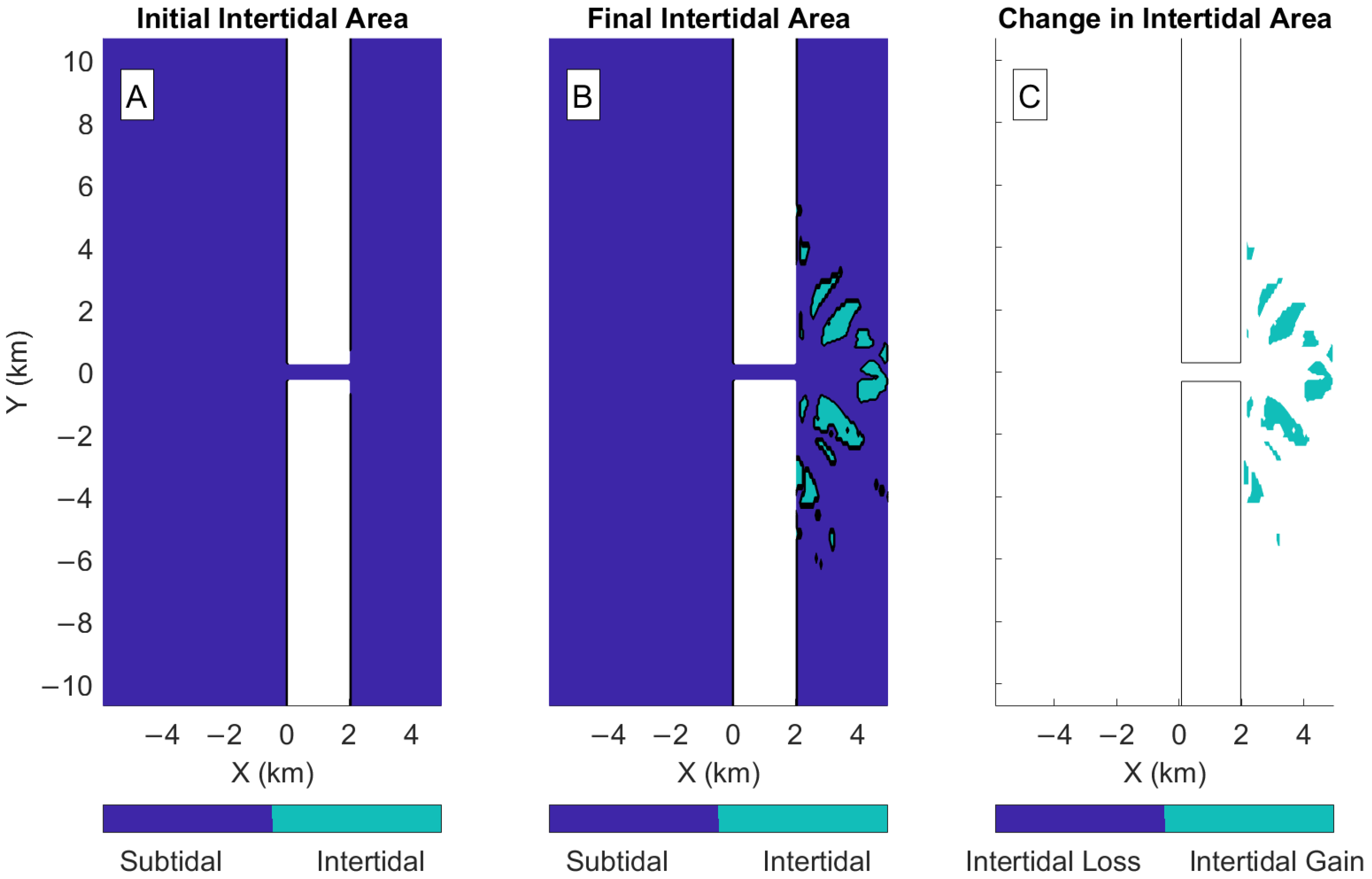
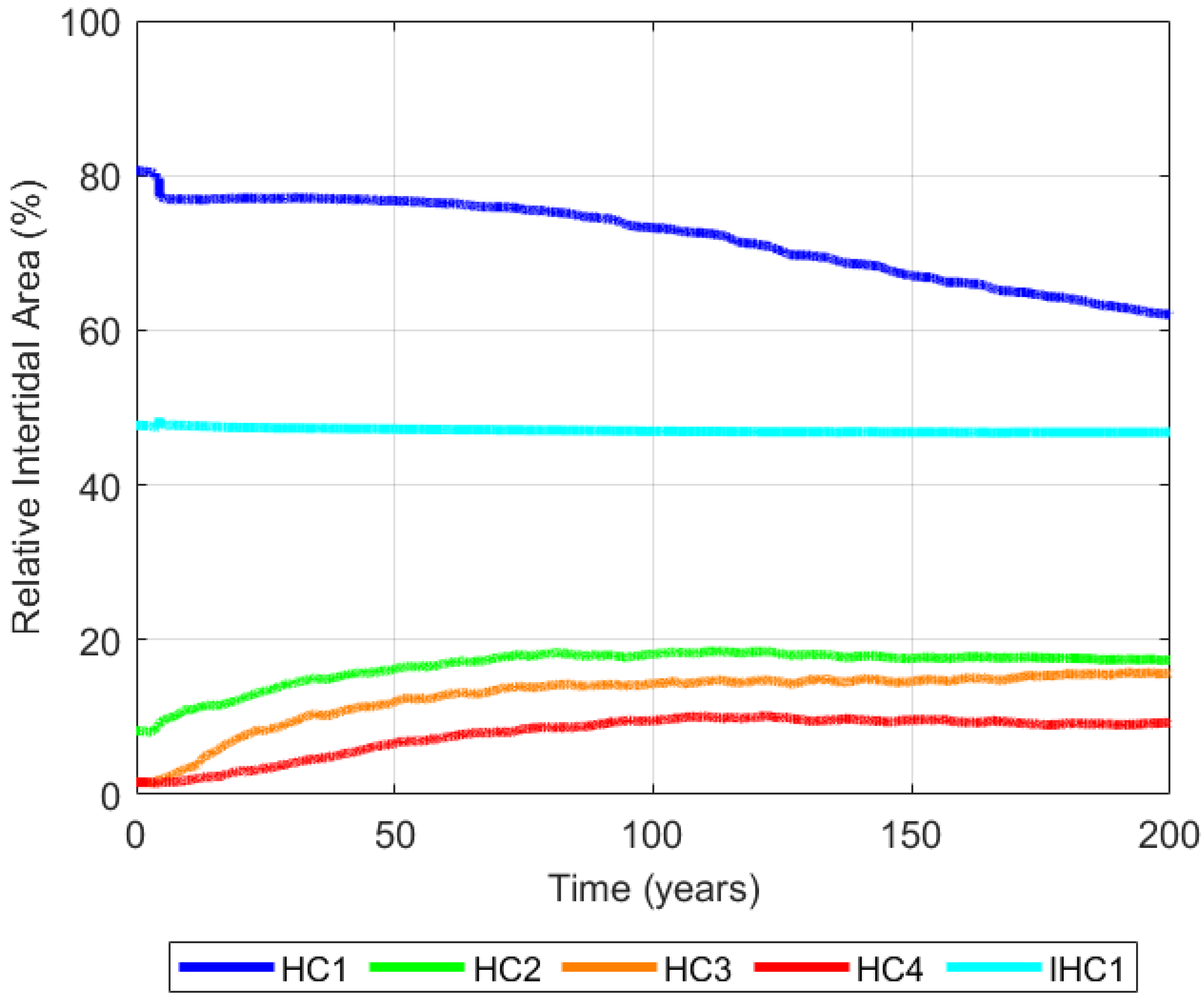
3.2.2. Relative Intertidal Area

Changes to relative intertidal area differ from changes to sediment volume in the bay, as both shoal formation or erosion and channel formation or deepening impact the sediment budget (Figure 20 and Figure 21). The continuous export of sediment from the bay in HC1 only impacts intertidal area abruptly in the first 5 years of simulation and after 75 years. Although IHC1 also loses sediment throughout the simulation, much of this erosion results in lower intertidal area over a relatively constant fraction of the bay. HC2 maintains a similar volume of sediment in the bay as intertidal area increases and loses sediment when the intertidal area stops being added. Net sediment flux into the bay follows a similar trend to intertidal area change in HC3 and HC4, but sediment flux rates into the bay decrease before the rate of intertidal area growth approaches zero. Simulations do not appear to approach a single intertidal area, so initial bathymetry conditions likely impact the achievable relative intertidal area.

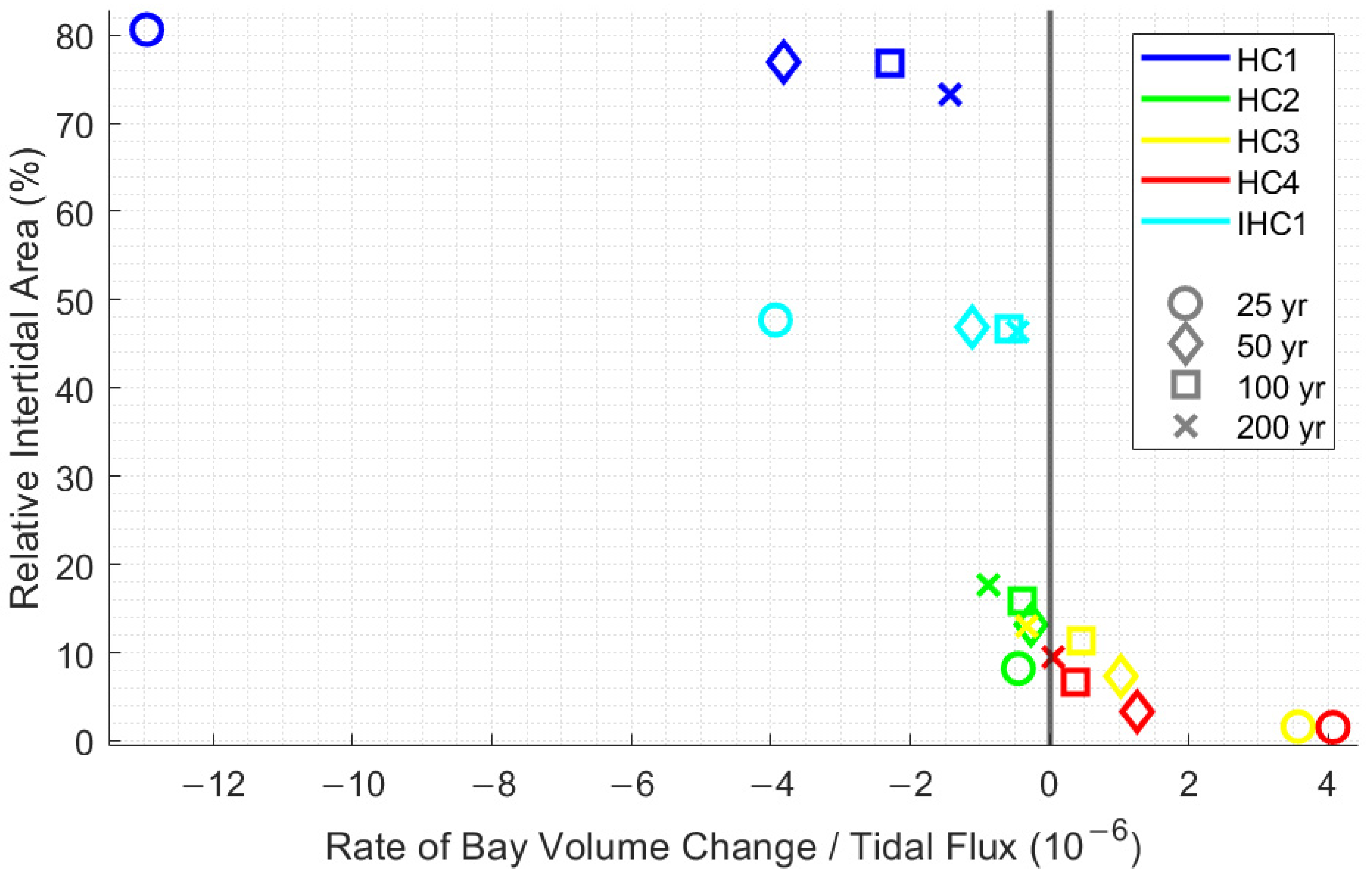
3.2.3. Intertidal Area vs. the Rate of Bay Volume Change

A relationship between intertidal area and ebb-dominant sediment transport has been observed in numerous studies (e.g., [3,4,5,36,37,38]). In these examples, the presence and extent of intertidal flats were related to ebb dominance. The intertidal area is compared to tidal asymmetry in more detail in Section 3.3, but net sediment transport to or from the bay is also found to have some dependence on intertidal area in the tested simulations. The rate of morphodynamic change was considered between 0, 25, 50, 100, and 200 years and compared with the average intertidal area. Morphodynamic change rates are normalized by the mean tidal flux through the inlet. Intertidal area is normalized by the area of the bay and averaged between the two time-steps represented in the volume change. The volume of sediment imported into the bay generally decreases with increasing intertidal area, with predominantly sediment import where approximately ≤10% of the bay was intertidal (Figure 22). The rate of sediment import decreases as cases that import sediment gain intertidal area, with HC3 exporting sediment by the end of the simulation. Cases that export sediment do export less sediment as intertidal decreases. The rates at which sediment is exported from the bay are generally much greater when more than ~60% of the bay is intertidal. The rates at which sediment is imported into the bay are greatest when the bay has no intertidal area and decrease as the bay gains intertidal area until about 10% of the bay is intertidal.

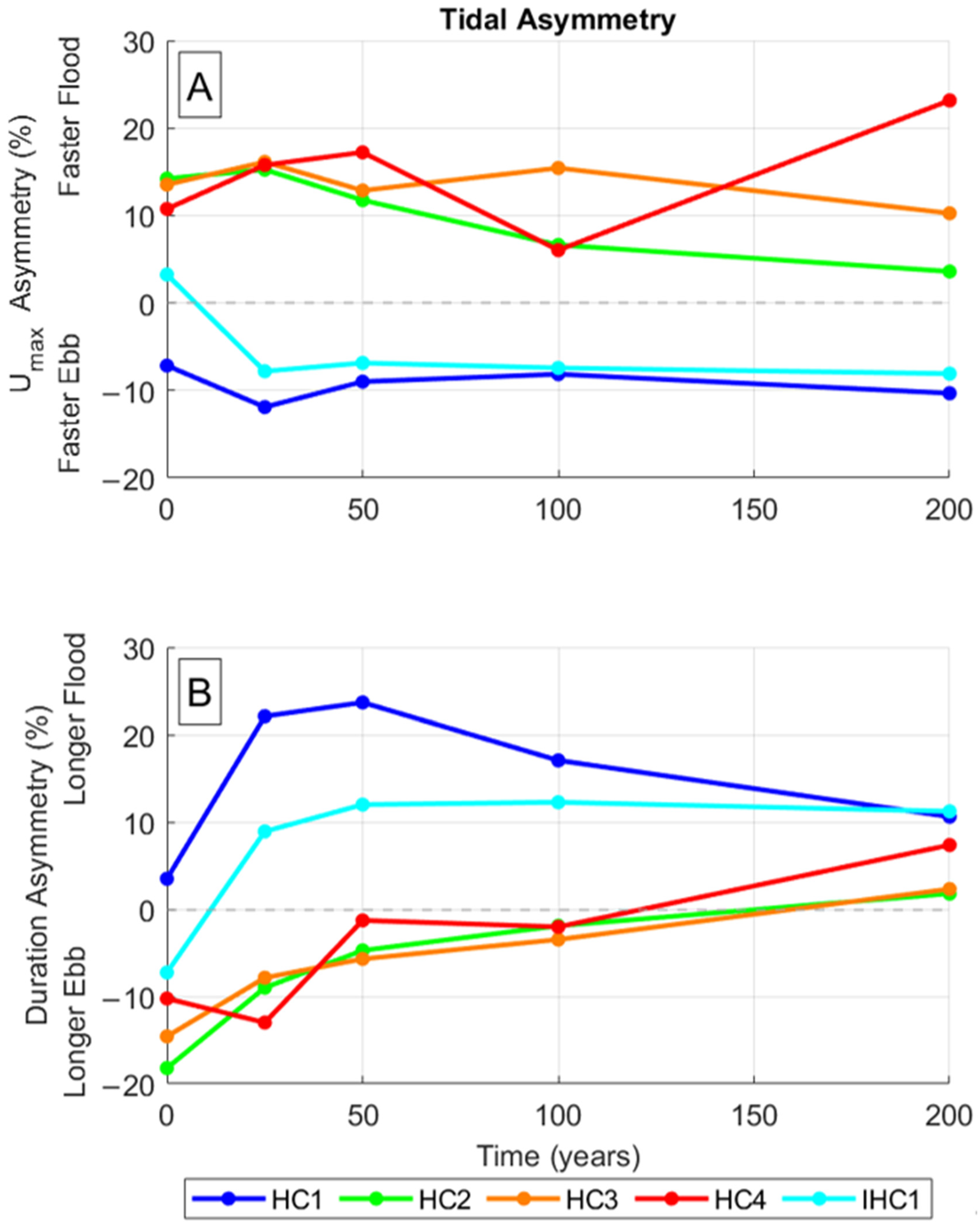
3.3. Tidal Asymmetry

Tidal asymmetry in the inlet was calculated to compare to net sediment transport direction and erosion/accretion patterns in the bay. Tidal asymmetry was quantified with two parameters: peak velocity asymmetry and tidal duration asymmetry. These quantities were calculated from spatial averages across the inlet in shorter 1-year simulations with 5 min save-point time-steps, but without waves or sediment transport. Simulations were run using the 0-, 25-, 50-, 100-, and 200-year bathymetry for each case. Peak velocity asymmetry indicates how much faster the fastest velocities were in the ebb or flood tide. As an example, a value of 10% represents a scenario in which peak ebb velocities are 10% faster than peak flood velocities. Tidal duration asymmetry indicates how much longer the ebb or flood tide lasted. As an example, a value of 15% corresponds to a scenario in which the flood tide is 15% longer than the ebb tide.

3.3.1. Peak Velocity and Tidal Duration Asymmetry

Peak velocity asymmetries are less than 25% in all cases and, with the exception of the initial conditions for IHC1, do not change direction (Figure 23A). Both HC1 and IHC1 have ebb dominant peak velocities, but HC1 is marginally more ebb asymmetric. The initial bathymetry in IHC1 makes peak velocities in the inlet flood dominant, but after 25 years, this has reversed and IHC1 remains ebb dominant for the remainder of the simulation. The initially sharp connections between the relatively tall intertidal areas and the channel connecting to the inlet may have some similarities to other findings linking friction between the inlet and bay to flood dominance (e.g., [39,40]). After hydrodynamic forcing reorganized a sufficient volume of sediment, IHC1 becomes ebb dominant. Peak ebb velocity asymmetry values range from 7 to 12% during the majority of each simulation. Peak velocities are flood dominant in HC2, HC3, and HC4, but are not clearly ranked until more than 100 years of morphology change have occurred. By the end of the simulation, peak velocities are more flood dominant in HC4 than in HC3 or HC2. Peak velocity asymmetry throughout the simulation matches net sediment transport direction to or from the bay in all cases but HC2.

Tidal duration asymmetries are similar to peak velocity asymmetries but have notable differences (Figure 23B). Tidal duration asymmetries in HC1 and IHC1 are similar to peak velocity asymmetry, but with larger magnitudes. The faster ebb velocities are related to a larger magnitude increase in the duration of flood tide. Ebb tides begin 10 to 20% longer than flood tides in HC2, HC3, and HC4, but this asymmetry reduces over the course of the simulation. The final morphologies cause 1 to 2% longer flood tides in HC2 and HC3, but 7% longer flood tides in HC4. This results in longer flood tides with faster peak velocities, but HC2 exports sediment from the bay and HC3 and HC4 have little net sediment transport to or from the bay. Net sediment transport must also depend on factors other than tidal asymmetry in the inlet.

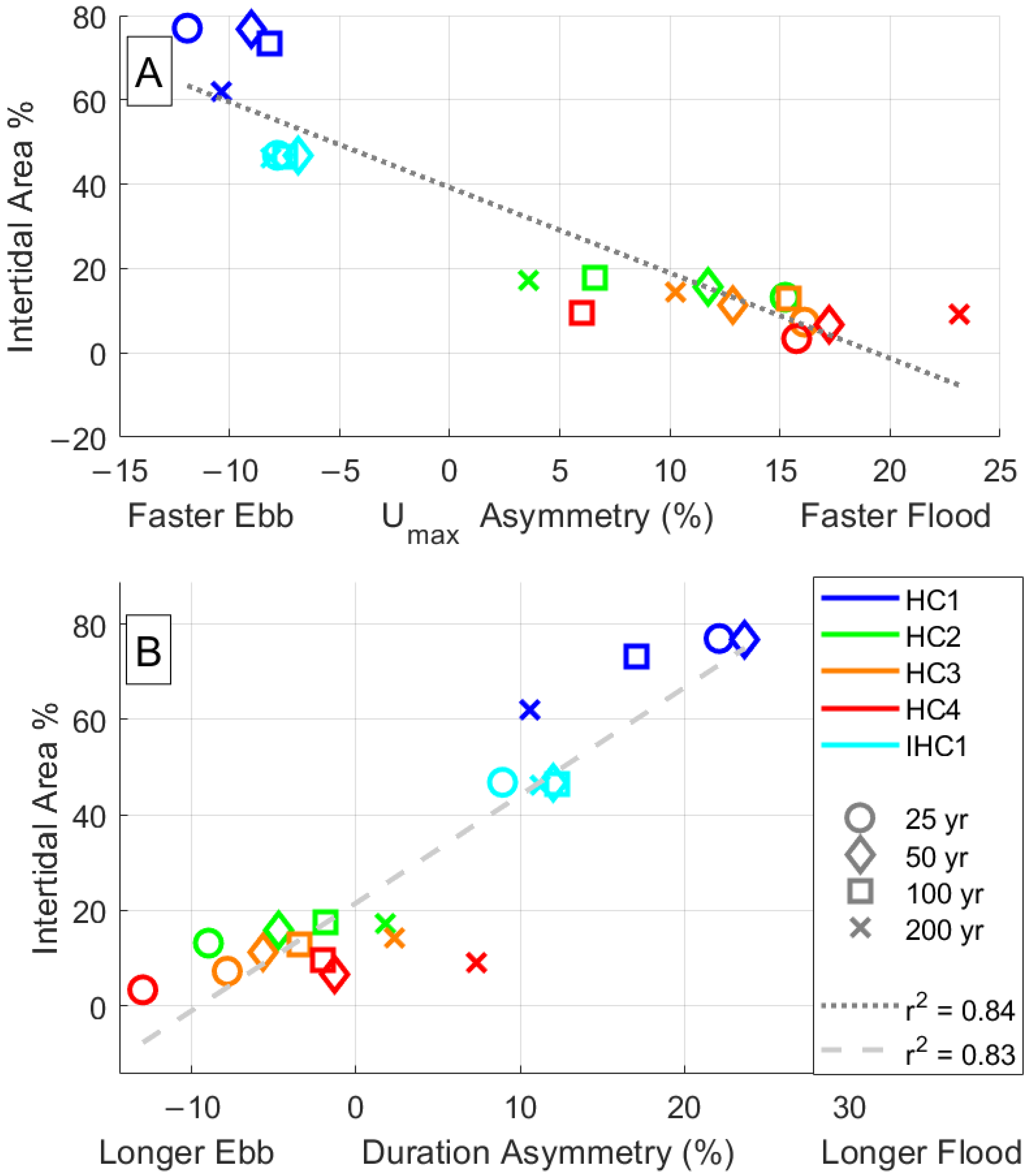
3.3.2. Tidal Asymmetry vs. Intertidal Area

Tidal asymmetry in the inlet was found to correlate to some degree with the intertidal area after an initial equilibration (Figure 24). The relatively angular starting bathymetry of the cases with much more sediment in the bay (i.e., HC1 and IHC1) appears to have had a large impact on tidal asymmetry, which was not reflected in other results. Although tidal asymmetry associated with the initial bathymetry in HC1 and IHC1 was weakly ebb dominant and weakly flood dominant, respectively, the intertidal area decreased and the bay exported sediment quickly. The large change in tidal asymmetry by the 25th year of the simulation indicates that the asymmetry changed with the rapidly changing morphology. After the first 25 years, bathymetry with much intertidal area corresponded to faster and shorter ebb flows through the inlet and cases with less intertidal area had slower and longer ebb flows through the inlet (Figure 24). Linear regression skills were evaluated to compare correlations between the intertidal area and the rate of volume change (Figure 22, R² = 0.53), peak velocity asymmetry (Figure 24, R² = 0.85), and tidal duration asymmetry (Figure 24, R² = 0.83). This relationship was not observed in the tidal asymmetry related to the initial bathymetry for HC1 and IHC1.

Tidal asymmetry depends on a variety of factors beyond intertidal area, but the results generally match previous findings that shoal formation and tidal flats shorten ebb tides (e.g., [5,7,36,37,38]). Peak velocity asymmetry after the first 25 years was found to have the highest correlation with the intertidal area of the considered traits. Peak velocity asymmetry and duration asymmetry are not expected to be entirely independent but were only correlated with an R² of 0.74 across the same data, indicating some independent correlation of each with intertidal area.

3.4. Hypsometry

Hypsographic curves were developed for each simulation by determining the area above each depth within the bay. Differences between hypsometry at the beginning and end of the simulation describe the changes in bay elevation distribution after 200 years of morphodynamic forcing. Hypsographic curves indicate the distribution of depths throughout the bay, but do not describe horizontal positions. The comparison of initial and final hypsographs demonstrates net gain or loss of area above each elevation. Bay hypsometry changes resulting from the differences in the starting bathymetry follow one of two general patterns. Channels connecting the inlet to the rest of the bay deepen to similar depths in all cases. Flood-dominant cases (HC2, HC3, and HC4) generally deposit sediment in areas outside of channels. Ebb-dominant cases (HC1 and IHC1) generally erode sediment from the intertidal areas. Tidal asymmetry is discussed in greater detail in Section 3.3. The hypsometry from the beginning and end of each simulation are grouped by tidal asymmetry in the inlet.

3.4.1. Hypsometry in Ebb-Dominant Simulations

Ebb-dominant cases export sediment. Some of the additional sediment in the bay at the start of the simulation is eroded. In HC1, elevations reduced over much of the bay. The intertidal areas lowered, and the channel narrowed and deepened. These morphological changes are demonstrated in Figure 25. In IHC1, elevations within the bay also reduced, but approximately two-thirds of the bay remained at similar elevations (Figure 26). Erosion predominantly occurred at intertidal depths and in the area immediately adjacent to the inlet.

3.4.2. Hypsometry in Flood-Dominant Cases

Flood-dominant cases contain large areas of both erosion and accretion within the bay. Erosion in flood-dominant cases is almost exclusively confined to the networks of channels that form. Sediment accretes between these channels. The balance between the channel and shoal formation determines the net sediment transport direction through the inlet. Although elevations in HC2 increase or remain the same across >75% of the bay, channel formation in approximately 12% of the bay drives net sediment export from the bay (Figure 27). In HC3, elevations increased or remained the same over approximately 80% of the bay (Figure 28), and the intertidal fraction of the bay increased throughout the simulation. The channels that form in HC3 have similar depths to the other cases, but are distributed between multiple somewhat narrower channels, occupying a slightly smaller fraction of the bay. In the Hypsometry Case 4 (HC4) simulation, channel formation and deepening occurred across approximately 12% of the bay, while accretion occurred across ~48% of the bay. The remaining portions showed little change in elevations (Figure 29). The volume of sediment in the bay increased more in HC4 than in HC3 over a smaller area, but final elevations were lower and less area was intertidal.

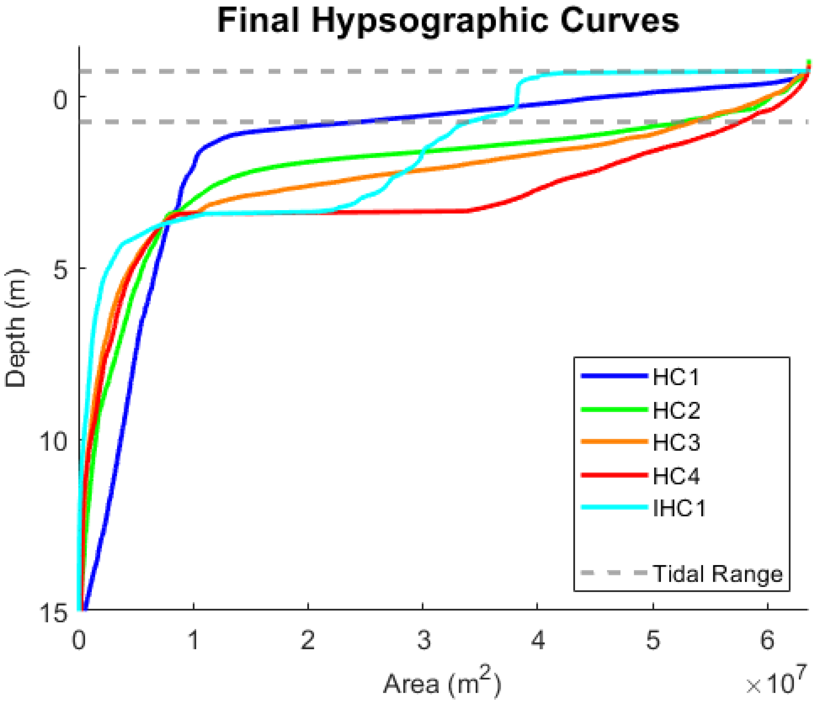
3.4.3. Hypsometry Convergence and Dependence on Initial Bathymetry

Hypsographs become more similar among cases over the course of each simulation, but important differences remain (Figure 30). Similar fractions of the bay are above the 3.7 m depth contour, but deeper depths vary and shallower depths vary greatly. The channelized flow of HC1 results in deep channels that occupy a similar area to the channels that form in other cases. The lack of a long channel network in IHC1 (Figure 17) is also evident in the final hypsography comparisons. Channel dimensions and locations in the bay vary greatly between HC2, HC3, and HC4 (Figure 11, Figure 13 and Figure 15), but the associated final hypsographs are particularly similar for depths below 3.7 m, indicating similar elevation distributions. The net import or export of sediment from the bay reduces and stabilizes over time in HC3 and HC4 (Figure 20C), so hypsometries are not expected to converge noticeably further over a longer time span and variations in the starting bathymetry are indicated to have permanent impacts on the hypsometry.

4. Discussion

4.1. Implications of Basin Hypsometry to Navigation

Initial hypsographic curves labeled HC1–HC4 were constructed to produce morphologies that transition from an estuary with extensive inter-tidal flats (HC1) to an estuary devoid of inter-tidal flats (HC4). These cases were chosen under the assumption that most lagoonal-type bar-built estuaries exist between these two extremes, and that modeling a family of morphological types within this range could offer an insight into a wide class of possible inlet system behavior. The theory implies that tidal asymmetry measured as the difference between the maximum flood/ebb velocities in the inlet throat should shift from ebb dominated (HC1) to flood dominated (HC4) [5]. The model results agree with the theory, as HC1 is ebb dominated, and HC2, HC3, and HC4 progressively become more flood dominated. Correspondingly, the idealized model setup, which is initially unbalanced in terms of total sediment volume within the estuary versus tidal prism, allows for basin-scale adjustments through the redistribution of sediment and corresponding changes in morphology and hypsometry consistent with theoretical predictions. While the final hypsometry, and associated morphology differ, all four cases tend to an equilibrium, in which sediment import or export relaxes asymptotically to a near-zero net gain or loss.

The majority of basin sediment loss for systems that export sediment is in the sub-tidal areas and regions that are lower in the tidal frame (HC1). This tends to deepen the basin by the preferential erosion of the sub-tidal areas. This could suggest little change in creek network structure and the size and distribution of tidal flats, while deepening sub-tidal channels. As the initial bay configuration begins to switch towards sediment import (HC2), subtidal erosion continues, but sediment also deposits on shallower subtidal areas, building an extensive network of intertidal shoals. The balance between channel erosion and shoal formation tips as subtidal areas are initially deeper (HC3). This becomes more pronounced with greater area increases for bays initially devoid of inter-tidal flats (HC4), but there are also greater gains in the sub-tidal areas decreasing the average bay depth. The increase in inter-tidal areas reduces the tendency to import sediment, producing feedback that supports an equilibrium configuration and a resulting basin with more tidal flats dissected by a dendritic creek network.

Lagoonal-type estuaries that are deeper and devoid of extensive tidal flats tend to promote sediment import and have a greater propensity to provide material that could exacerbate channel shoaling. Activities, such as wetland mining, channel deepening and other engineering projects that remove sediment and reduce the inter-tidal footprint, could increase the rate of sediment import. By the same token, lagoonal-type estuaries that deepen due to sea level rise would similarly have the potential for greater sediment import and increased shoaling rates.

On the other hand, lagoonal-type estuaries with extensive inter-tidal flats create ebb-dominated currents that promote the export of sediment. Material removed from channels during dredging and placed strategically in other energetic regions within the estuary would have a greater chance of leaving the system as opposed to returning to the channel. The results (HC1) show a greater sediment loss in the deeper section of the system, so any tendency for channel shoaling is at least partially offset by the net erosion and export of sediment.

4.2. Implications of Sediment Placement in Inter-Tidal Areas to Navigation

HC1 may represent several important features of the back-barrier response to systems in which the majority of new material is placed on the existing flats in the inter-tidal zone. Morphology change in HC1 is predominantly channel deepening, with a smaller volume of sediment eroded from the intertidal flats. Additionally, channels that deepen along the extensive intertidal areas of HC1 and the shallow sub-tidal areas of HC2 are deeper and extend farther back into the bay than the channels that form in the relatively deep subtidal areas of HC3 or the flat featureless bathymetry of HC4. Erosion is predominantly from the channel in HC1 and HC2, but the extensive intertidal areas of HC1 continue to erode later in the simulation after the channel has stabilized.

In real-world systems, this pattern of channel erosion adjacent to large intertidal areas is sometimes explained by a shift in the timing of maximum ebb and flood currents, so that peak vertical shear reduces during flood and increases during ebb (e.g., [41]). The greater ebb turbulence and shear stress can help to contribute to the increased bottom friction and sediment transport during ebb tide [41]. If peak velocities are shifted late enough in the ebb tide, many intertidal areas may be exposed and erosion may occur in the channels as opposed to occurring on the flats.

4.3. Implications of Land Reclamation to Navigation

IHC1 can be viewed as a rudimentary model of how a lagoonal-type inlet may respond to a land reclamation project, in which material is used to create new land by raising the bed elevation above tidal and storm influence. Many long-term land reclamation projects reduce overall bay volume [42], primarily in the shallow and inter-tidal areas near adjacent shorelines, while leaving the deeper areas relatively undisturbed.

Most of the sediment loss occurs in the inter-tidal zone, but in such a way that preserves the overall inter-tidal area, i.e., the inter-tidal zone is nearly constant over the 200-year simulation (30.5 to 29.5 km²). Sediment eroded from the inter-tidal zone is exported and bypasses the deeper sections of the bay as indicated by the lack of significant change in the hypsometry in the sub-tidal areas (except in the small region adjacent to the inlet throat). Land reclamation may increase the rate of edge erosion and trend toward steeper side slopes in channels, which could promote unstable conditions. The fact that the erosion is primarily confined to the inter-tidal zone will reduce the area of tidal flats, of which an extreme example would be the removal of all wetlands, leading to open water throughout the basin.

4.4. Sediment Flux versus Intertidal Area

The net rate of sediment flux through the inlet is a function of not only the temporal evolution of the basin morphology, in which the rate slows as the system asymptotically approaches a neutral configuration, but also the size of the inter-tidal and sub-aqueous areas (Figure 22). The highest sediment flux occurs when the inter-tidal area is either less than ~10% (import) or greater than ~60% (export) of the total basin area. If the inter-tidal area lies between 10% and 60%, the import and export rates are reduced and the inlet approaches a stable morphological configuration with a vanishingly small net transport. While the results are limited by the small number of conditions that were modeled, this concept can easily be developed further by modeling many systems and researching inter-tidal coverage in real inlets and correlating that to sediment import and export rates. Further investigation could reinforce this concept, leading to a new metric to determine the relationship between large-scale wetland or land reclamation and changes in channel shoaling patterns that would be very beneficial to future navigation project planning studies.

5. Conclusions

Increasing societal pressures (e.g., population growth and urbanization) are driving land use change practices in coastal areas and potentially will affect the hydrodynamics and sediment transport in ways that might exacerbate the existing shoaling issues. To understand the potential impact of coastal development better, a numerical model was used to predict the long-term evolution of a lagoonal-type barrier island inlet under a set range of morphological conditions that transitioned from net sediment import to net sediment export. Two of the model simulations, HC1 and IHC1, were further analyzed to examine the effect of inter-tidal placement, one in which the majority of material was restricted to elevations high in the tidal frame (IHC1).

The results indicate that the likelihood of channel shoaling may be greater for large-scale inter-tidal placement projects. Inter-tidal placement tends to enhance erosion in the sub-aqueous regions and the deeper portion of the inter-tidal zone. This may reduce the rate of new wetland erosion but lead to greater sediment deposits in the deeper channels, where it could increase channel shoaling. Placing material high in the tidal frame leads to greater erosion of the inter-tidal zone, with sediment bypassing the deeper sections. This could reduce the size of tidal flats but produce less sediment deposition in navigation channels. Furthermore, the numerical model results indicated that basins devoid of inter-tidal areas tended to import sediment, decreasing the overall channel depth and increasing inter-tidal areas. This suggests increased channel shoaling and larger tidal flats.

A noteworthy result is the relationship between inter-tidal area and sediment transport. If the inter-tidal area comprises a very small portion of the total area (<~10%), then the system tends to import sediment. This effectively decreases basin depth and increases the inter-tidal footprint, which shifts the system towards neutral conditions (zero net sediment import/export). If the inter-tidal area comprises a large portion of the total area (>~60%), the system tends to export sediment. This conclusion is based on a small number of numerical modeling cases, and should be viewed as preliminary. However, increasing the number of inlet types is relatively straightforward, so further examination on this concept is very feasible and could offer an efficient way to examine the impacts on navigation for a wide variety of systems using very simple metrics.

References

- Komar, P.D. Beach Processes and Sedimentation, 2nd ed.; Prentice Hall: Upper Saddle River, NJ, USA, 1998. [Google Scholar]
- Inniss, L.; Simcock, A.; Ajawin, A.Y.; Alcala, A.C.; Bernal, P.; Calumpong, H.P.; Araghi, P.E.; Green, S.O.; Harris, P.; Kamara, O.K.; et al. The First Global Integrated Marine Assessment; United Nations: New York, NY, USA, 2016; Volume 1, p. 23, Volume 4, p. 6. [Google Scholar]
- Dronkers, J. Tidal Asymmetry and Estuarine Morphology. Neth. J. Sea Res. 1986, 20, 117–131. [Google Scholar] [CrossRef]
- Friedrichs, C.T.; Aubrey, D.G. Non-Linear Tidal Distortion in Shallow Well-mixed Estuaries: A Synthesis. Estuar. Coast. Shelf Sci. 1988, 27, 521–545. [Google Scholar] [CrossRef]
- Speer, P.; Aubrey, D. A study of non-linear tidal propagation in shallow inlet/estuarine systems Part II: Theory. Estuar. Coast. Shelf Sci. 1985, 21, 207–224. [Google Scholar] [CrossRef]
- Strahler, A.N. Hypsometric (area-altitude) analysis of erosional topography. Geol. Soc. Am. Bull. 1952, 63, 1117–1142. [Google Scholar] [CrossRef]
- Boon, J.D.; Byrne, R.J. On basin hypsometry and the morphodynamic response of coastal inlet systems. Mar. Geol. 1981, 40, 27–48. [Google Scholar] [CrossRef]
- Townend, I.H. Hypsometry of Estuaries, Creeks and Breached Sea Wall Sites. Proc. Inst. Civ. Eng.-Marit. Eng. 2008, 161, 23–32. [Google Scholar] [CrossRef]
- Leuven, J.R.; Selakovic, S.; Kleinhans, M.G. Morphology of bar-built estuaries: Empirical relation between planform shape and depth distribution. Earth Surf. Dyn. 2018, 6, 763–778. [Google Scholar] [CrossRef] [Green Version]
- Thorne, K.M.; MacDonald, G.M.; Ambrose, R.F.; Buffington, K.J.; Freeman, C.M.; Janousek, C.N.; Brown, L.N.; Holmquist, J.R.; Guntenspergen, G.R.; Powelson, K.W.; et al. Effects of Climate Change on Tidal Marshes along a Latitudinal Gradient in California (No. 2016-1125); US Geological Survey: Reston, VA, USA, 2016. [CrossRef] [Green Version]
- Blanton, J.O.; Lin, G.; Elston, S.A. Tidal Current Asymmetry in Shallow Estuaries and Tidal Creeks. Cont. Shelf Res. 2002, 22, 1730–1743. [Google Scholar] [CrossRef]
- Guo, L.; Brand, M.; Sanders, B.F.; Foufoula-Georgiou, E.; Stein, E.D. Tidal asymmetry and residual sediment transport in a short tidal basin under sea level rise. Adv. Water Resour. 2018, 121, 1–8. [Google Scholar] [CrossRef]
- Cayocca, F. Long-term morphological modeling of a tidal inlet: The Arcachon Basin, France. Coast. Eng. 2001, 42, 115–142. [Google Scholar] [CrossRef]
- Dissanayake, D.; Roelvink, J.; Van der Wegen, M. Modelled channel patterns in a schematized tidal inlet. Coast. Eng. 2009, 56, 1069–1083. [Google Scholar] [CrossRef]
- Yu, Q.; Wang, Y.; Flemming, B.; Gao, S. Scale-dependent characteristics of equilibrium morphology of tidal basins along the Dutch-German North Sea Coast. Mar. Geol. 2014, 348, 63–72. [Google Scholar] [CrossRef]
- Boelens, T.; Qi, T.; Schuttelaars, H.; De Mulder, T. Morphodynamic equilibria in short tidal basins using a 2DH exploratory model. J. Geophys. Res. Earth Surf. 2021, 126, e2020JF005555. [Google Scholar] [CrossRef]
- Nahon, A.; Bertin, X.; Fortunato, A.B.; Oliveira, A. Process-based 2dh morphodynamic modeling of tidal inlets: A comparison with empirical classifications and theories. Mar. Geol. 2012, 291, 1–11. [Google Scholar] [CrossRef]
- Van der Wegen, M.; Roelvink, J.A. Long-term morphodynamic evolution of a tidal embayment using a two-dimensional, process-based model. J. Geophys. Res. Oceans 2008, 113, C3. [Google Scholar] [CrossRef] [Green Version]
- Styles, R.; Brown, M.E.; Brutsché, K.E.; Li, H.; Beck, T.M.; Sánchez, A. Long-Term Morphological Modeling of Barrier Island Tidal Inlets. J. Mar. Sci. Eng. 2016, 4, 65. [Google Scholar] [CrossRef] [Green Version]
- Dean, R.G.; Dalrymple, R.A. Coastal Processes with Engineering Applications; Cambridge University Press: Cambridge, UK, 2004. [Google Scholar]
- van Rijn, L. Two-Dimensional Vertical Mathematical Model for Suspended Sediment Transport by Currents and Waves; Report S488-IV; Delft Hydraulics: Delft, The Netherlands, 1985. [Google Scholar]
- National Oceanic and Atmospheric Administration. Harmonic Constituents for 9418767, North Spit CA. Available online: https://tidesandcurrents.noaa.gov/harcon.html?unit=0&timezone=0&id=9418767&name=North+Spit&state=CA (accessed on 28 February 2022).
- Rosati, J.D.; Walton, T.L.; Bodge, K. Longshore Sediment Transport. In Coastal Engineering Manual, Part III, Coastal Sediment Processes, III-2-2, EM 1110-2-1100; U.S. Army Corps of Engineers: Washington, DC, USA, 2002. [Google Scholar]
- Baar, A.W.; Boechat Albernaz, M.; Van Dijk, W.M.; Kleinhans, M.G. Critical dependence of morphodynamic models of fluvial and tidal systems on empirical downslope sediment transport. Nat. Commun. 2019, 10, 4903. [Google Scholar] [CrossRef] [Green Version]
- LeConte, L.J. Discussion of Notes on the improvement of river and harbor outlets in the United States. Trans. Am. Soc. Civ. Eng. 1905, 55, 306–308. [Google Scholar] [CrossRef]
- O’Brien, M.P. Estuary tidal prisms related to entrance areas. Civ. Eng. 1931, 1, 738–739. [Google Scholar]
- O’Brien, M.P. Equilibrium flow areas of inlets on sandy coasts. J. Waterw. Harb. Div. Am. Soc. Civ. Eng. 1969, 96, 43–52. [Google Scholar] [CrossRef]
- Jarrett, J.T. Tidal Prism-Inlet Area Relationships. In GITI Report 3; U.S. Army Corps of Engineers: Vicksburg, MS, USA, 1976. [Google Scholar]
- Walton, T.L.; Adams, W.D. Capacity of Inlet Outer Bars to Store Sand. Coast. Eng. Proc. 1976, 1, 1919–1937. [Google Scholar] [CrossRef]
- Hicks, D.M.; Hume, T.M. Morphology and Size of Ebb Tidal Deltas at Natural Inlets on Open-Sea and Pocket-Bay Coasts, North Island, New Zealand. J. Coast. Res. 1996, 12, 47–63. Available online: https://www.jstor.org/stable/4298459 (accessed on 16 March 2022).
- Wright, L.D. Sediment transport and deposition at river mouths: A synthesis. Geol. Soc. Am. Bull. 1997, 88, 857–868. [Google Scholar] [CrossRef]
- Edmonds, D.A.; Slingerland, R.L. Mechanics of river mouth bar formation: Implications for the morphodynamics of delta distributary networks. J. Geophys. Res. Earth Surf. 2007, 112, F2. [Google Scholar] [CrossRef] [Green Version]
- Beck, T.M.; Kraus, N.C. Ebb-tidal delta development where before there was none, Shark River Inlet, New Jersey. Proc. Coast. Sediments 2011, 3, 458–471. [Google Scholar] [CrossRef]
- Beck, T.M.; Kraus, N.C. New ebb-tidal delta at an old inlet, Shark River Inlet, New Jersey. J. Coast. Res. 2011, 59, 98–110. [Google Scholar] [CrossRef]
- Fagherazzi, S.; Edmonds, D.A.; Nardin, W.; Leonardi, N.; Canestrelli, A.; Falcini, F.; Jerolmack, D.J.; Mariotti, G.; Rowland, J.C.; Slingerland, R.L. Dynamics of river mouth deposits. Rev. Geophys. 2015, 53, 642–672. [Google Scholar] [CrossRef] [Green Version]
- van Maanen, B.; Coco, G.; Bryan, K.R. Modelling the effects of tidal range and initial bathymetry on the morpho-logical evolution of tidal embayments. Geomorphology 2013, 191, 23–34. [Google Scholar] [CrossRef]
- Boelens, T.; Schuttelaars, H.; Schramkowski, G.; De Mulder, T. The effect of geometry and tidal forcing on hydrodynamics and net sediment transport in semi-enclosed tidal basins. Ocean. Dyn. 2018, 68, 1285–1309. [Google Scholar] [CrossRef]
- Robins, P.E.; Davies, A.G. Morphological controls in sandy estuaries: The influence of tidal flats and bathymetry on sediment transport. Ocean. Dyn. 2010, 60, 503–517. [Google Scholar] [CrossRef]
- Lanzoni, S.; Seminara, G. On tide propagation in convergent estuaries. J. Geophys. Res. Ocean. 1998, 103, 30793–30812. [Google Scholar] [CrossRef]
- Seabergh, W.C.; Cialone, M.A.; McCormick, J.W.; Watson, K.D.; Chasten, M.A. Monitoring Barnegat Inlet, New Jersey, South Jetty Realignment; ERDC/CHL TR-03-9; Engineer Research and Development Center, Coastal and Hydraulics Lab.: Vicksburg, MS, USA, 2003. [Google Scholar]
- Traynum, S.; Styles, R. Exchange flow between two estuaries connected by a shallow tidal channel. J. Coast. Res. 2008, 24, 1260–1268. [Google Scholar] [CrossRef]
- Healy, G.M.; Hickey, K.R. Historic land reclamation in the intertidal wetlands of the Shannon estuary, western Ireland. J. Coast. Res. 2002, 36, 365–373. [Google Scholar] [CrossRef]