Article

Estimation of Total Suspended Matter Concentration of Ha Long Bay, Vietnam, from Formosat-5 Image

1
Department of Geomatics, National Cheng Kung University, Tainan 701, Taiwan
2
Department of Civil Engineering, Vietnam Maritime University, Haiphong City 180000, Vietnam
*
Author to whom correspondence should be addressed.
J. Mar. Sci. Eng. 2022, 10(3), 441; https://doi.org/10.3390/jmse10030441
Submission received: 23 January 2022 / Revised: 2 March 2022 / Accepted: 15 March 2022 / Published: 18 March 2022
(This article belongs to the Special Issue Satellite Monitoring of Ocean)

Abstract

:
This study proposes the use of spatial high-resolution Formosat-5 (FS5) images for estimating total suspended matter (TSM) concentrations in a coastal region. Although many atmospheric correction methods are available, none of them are proposed to apply to FS5. Therefore, to remove the atmospheric effect, we performed a linear regression between the digital number (DN) of an FS5 image and the Landsat-8 Operational Land Imager (OLI) level-2 remote-sensing reflectance (Rrs) by using 160 samples of five ground targets. The ground targets, namely roof material, asphalt, water, vegetation, and other materials (sand and soil), were assumed to have negligible differences within 24 h. The results show that the linear model used for computing FS5 reflectance exhibited good coefficients of determination (R2) ranging from 0.87 to 0.96 for blue, green, red, and near-infrared bands. Next, in situ TSM measurements were not collected during the FS5 overpassing in Ha Long Bay, Vietnam, so we used two existing algorithms with a red band to estimate the TSM concentration. These algorithms developed for different coastal waters exhibited satisfactory agreement between derived field data and observed TSM concentrations with R2 ranging from 0.86 to 0.95. We also cross-checked the accuracy of the FS5-derived TSM concentration through comparison with an OLI-derived TSM image. The OLI-derived TSM image was validated and discussed for Vietnamese coastal waters, including Ha Long Bay. Lastly, based on comparisons between FS5- and OLI-derived TSM images in terms of spatial distribution, histograms, and root mean square error, we indicated the FS5 images after the removal of atmospheric effects could be totally used for estimating TSM in coastal water regions.

1. Introduction

Total Suspended Matter (TSM), which may also be referred to as Suspended Particular Matter (SPM) or Total Suspended Solids (TSS), is a key part of studying coastal water regions areas such as bays, lagoons, and estuaries [1] because of its influence on the marine environment and ecosystems. For example, TSM concentration can affect the health of the ecosystem for oyster growth in a bay [2]. Therefore, studying TSM characteristics can help researchers to better understand the marine ecosystem and the coastal environment. There are many methods to investigate TSM in coastal water regions, such as site measurement, numerical models, remote sensing, etc. In situ measurements with cruise and numerical models are costly and time-consuming [3], while remote sensing provides a viable solution that saves time and cost [4]. Remote sensing currently offers new satellite images that contain richer spatial information and are able to overcome hardware and operational cost issues due to state-of-the-art technologies [5,6]. Therefore, we propose the advantages of remote sensing solution by using the new satellite images of the Formosat-5 sensor to study TSM in a coastal region.
Formosat-5 (FS5) is a Taiwanese satellite that was launched on 25 August 2017. FS5 is operated by the National Space Organization (NSPO), Taiwan, and continues the mission of its predecessor, Formosat-2 (FS2). The FS2 images are usually used as sources for cartography and cadastral mapping, coastal water areas, differentiating between soil and vegetation, forest type mapping, detecting cultural features, and satellite images for post-earthquake disaster assessment, etc. [7,8,9]. FS2 was decommissioned in August 2016, and now, FS5 is the next generation of satellites of FS2, so the satellite imaging applications of FS5 are similar to those of FS2 in order to continue the mission of the previous generation. For example, high-resolution FS2 remote-sensing images improved the monitoring of the coastal water environment [10], the Gaoping River mouth [11], and reservoir water quality in Taiwan [12]. Because FS2 images have not been available since August 2016, we propose the use of FS5 satellite images to estimate the total suspended matter (TSM) concentration in coastal regions.
We proposed FS5 instead of other sensors because FS5 offers 4 m spatial resolution and one-day revisiting time, which is suitable for investigating TSM in shallow water. Furthermore, even though FS5 is a new generation of FS2, there is no full research to use FS5’s image to study TSM in coastal water regions. Even though FS5 provides the advantages of spatial and temporal resolution, there are two main research issues we faced when choosing FS5 to estimate TSM in coastal waters including removing atmospheric influence on FS5 images and choosing a suitable algorithm to estimate TSM concentration.
Removal of the atmospheric effect from a satellite image is a crucial step prior to using it to evaluate the optical characteristics of water in coastal areas. Different atmospheric correction methods are available for different types of sensors used to study sediments in coastal water regions. For example, five atmospheric correction algorithms can be applied to optically complex ocean waters for the Sentinel-3A sensor [13]. A new atmospheric correction approach was proposed for turbid coastal waters that entails using Moderate Resolution Imaging Spectroradiometer (MODIS) imagery [14]. Many Landsat-8 operational land imager (OLI) atmospheric correction algorithms for inland and coastal waters have been reported [15,16]. Currently, the research problem is that none of them are applicable to the proposed FS5 because FS5 provides the band from the visible to near-infrared band. Therefore, our proposed research objective is the use of linear regression to convert a DN into remote-sensing reflectance (Rrs) for FS5 images because this method has been widely used for different sensors in various geographical areas. Linear regression can be performed by assuming that a linear relationship exists among ground targets. Linear regression has been used for many different sensors. For example, the empirical line method was applied to images of the Caribbean Islands captured from both the Sentinel-2A Multispectral Instrument [17] and IKONOS [18] and used for the calibration of the airborne Daedalus-Coastal Zone Color Scanner [19]. Another study employed a refined empirical line approach to retrieve the reflectance factor from the Landsat-5 Thematic Mapper and Landsat-7 Enhanced Thematic Mapper [20].
An empirical method is usually used to estimate the TSM concentration from satellite images. This method involves the use of in situ measurement data to develop algorithms on the basis of the relationship between the TSM concentration and either a single band or multiple bands of satellite images. For example, a single algorithm was developed to retrieve turbidity from remotely sensed data in all coastal and estuarine waters [21]. A simple empirical band ratio algorithm was used to examine suspended particulate matter from remote-sensing data obtained for the coastal and inland waters of Vietnam [22]. In addition, in remote sensing, MODIS Terra 250-m images with a practical algorithm were used to determine the TSS concentration in coastal [23] and shallow waters [4]. Even though the empirical method is easy to use if the available in situ measurement data match satellite images, this method is expensive, time consuming, and limited by spatial distribution. Therefore, multi-sensors are commonly used to estimate suspended sediments in coastal waters. For example, a study integrated MODIS and Formosa-2 imagery to develop a reliable and high temporal–spatial resolution TSM concentration retrieval model [10]. A multi-sensor approach was adopted to examine the distribution of TSM in the Albemarle–Pamlico estuarine system in the United States [24]. Furthermore, recent studies have used semi-empirical algorithms and artificial intelligence to estimate TSM. For example, a robust algorithm was developed to estimate total suspended solids (TSSs) in inland and coastal waters [25]. A semi-empirical algorithm based on the Sentinel-3 Ocean and Land Color Instrument was developed for turbid case-2 waters [26]. A study forecasted TSS concentration reservoirs in real time through the optimal integration of multiple machine learning techniques [27].
Due to the lack of match up situ measurement data with satellite images, many studies have applied algorithms developed for previous sensors to new sensors, which are similar in terms of spatial and spectral characteristics, to estimate the TSM concentration in different areas. The advantage of this approach is the use of an already developed and validated algorithm for a different sensor and a different region. The results have revealed the satisfactory performance of these algorithms when applied to coastal waters. For example, a simple algorithm was developed to retrieve TSM from the VNREDSat-1/NAOMI sensor over the coastal and inland waters of Vietnam; it was based on the four existing algorithms of SPOT 5 (Satellite Probatoire de l’Observation de la Terre) and Landsat-8 OLI [22]. An empirical algorithm developed specifically for the South Korean coastal with the Geostationary Ocean Color Imager sensor was used to estimate the TSS concentration for MODIS images in coastal Taiwan [28]. Another study employed a refined empirical line approach for the Landsat-7 Enhanced Thematic Mapper by retrieving the reflectance factor from the Landsat-5 Thematic Mapper [20]. Yang et al. (2018) estimated turbidity in a macro-tidal harbor of Australia by using an algorithm for different MODIS products (Aqua/Terra) [29]. A simple optical model from other sensors was used to estimate SPM by using Landsat 8 data in the Yellow River estuary [30,31].
The research issue is that an empirical algorithm that has not been developed to estimate the TSM concentration from the FS5 image. No in situ TSM measurements were collected during the FS5 overpassing the study area. Therefore, for the different reasons mentioned above, in this study, the research objective was to select two algorithms, which were developed for OLI and FS2, to estimate the TSM concentration in Ha Long Bay, Vietnam. These two algorithms were developed in different water regions, so they need to be validated by reference data such as in situ measurement data or comparison with other sensors algorithms, which have been validated in the study area. For that purpose, we performed a comparison with an OLI-derived TSM image to examine the accuracy of the TSM concentration because in situ measurement data were unavailable. There are two reasons that motivate us to choose the OLI-derived TSM image as the reference data. Particularly, studies use the OLI-derived TSM image, which was processed by using the ACOLITE application (the detail of ACOLITE is written in later in Section 3.1) and is being widely used for different shallow water regions such as Belgian turbid coastal waters [32], Shengjin Lake and Chaohu Lake in China [33], Gorky Reservoir in Russia [34], the Estuary Zone of the Mzymta River, Black Sea [35], a tropical Ramsar wetland of southern India [36], and Vietnamese coastal waters [37]. In addition, the algorithm (Nechad et al., 2010 [38]) was used by ACOLITE is an international algorithm that has been validated and discussed for the coastal area of Vietnam (including Ha Long Bay in this study) [22]. ACOLITE is widely accepted for different coastal areas in many parts of the world including coastal Vietnam. Therefore, we also chose OLI-derived TSM with ACOLITE as a possible alternative due to the lack of in situ measurement.
This paper is organized as follows: Section 2 describes the study area, satellite match-up data set and in situ measurement data, and materials. Section 3 explains the methodology, including data processing and the use of linear regression to convert a DN into Rrs, TSM algorithms, and accuracy assessment. Section 4 and Section 5 present the results and discussion related to FS5-derived TSM from Ha Long Bay, respectively. Finally, Section 6 provides the conclusion and suggestions that indicate the key findings of this study and issues that require attention.

2. Materials and Methods
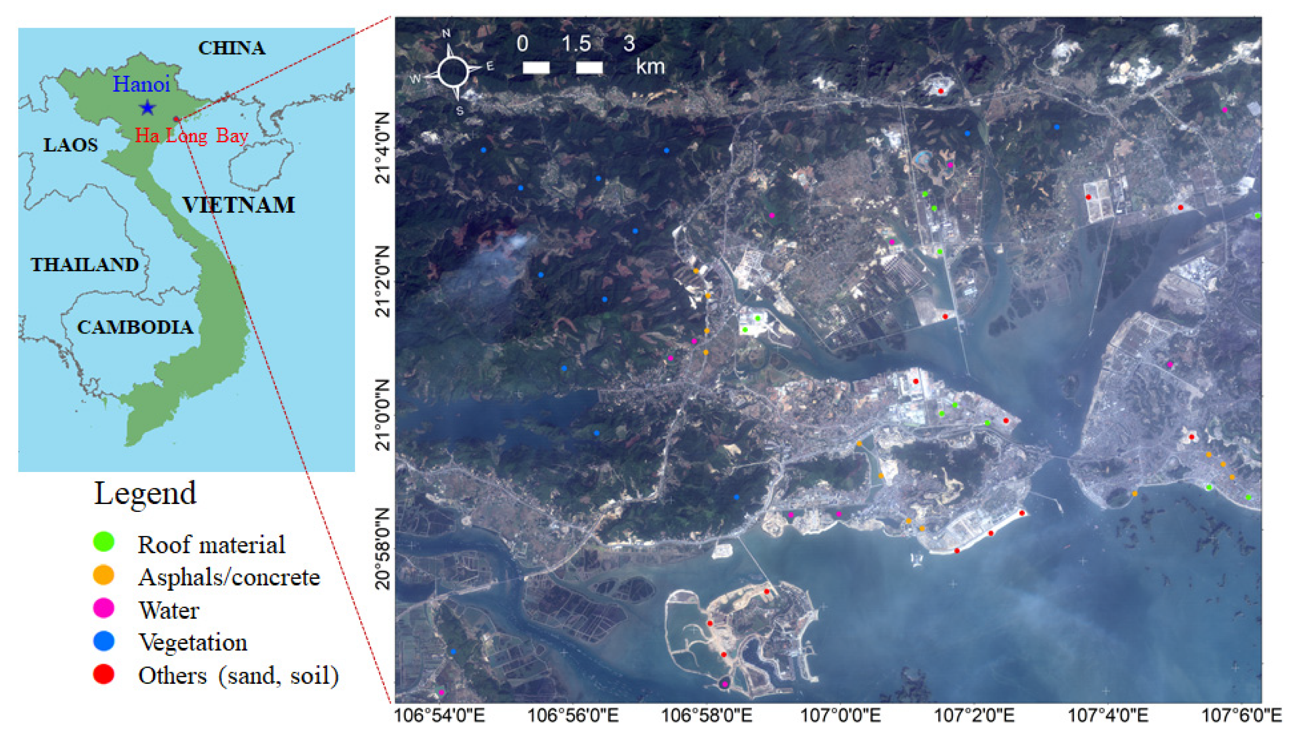
2.1. Study Area

Ha Long Bay, located in northern Vietnam, is one of the most popular travel destinations in Vietnam and a UNESCO World Heritage Site (Figure 1). The sediment characteristics of the Ha Long Bay area are those of an major marine environment topic because TSM is a critical parameter that affects water quality and environmental protection in Ha Long Bay [39,40].
We used data from previous studies that described the sediment characteristics of Ha Long Bay. According to the Ha Long Bay water quality management project [40], from 2004 to 2014, the average TSM concentration ranged from 16.1 to 35.08 mg/L with water depth in a range of 1–15 m. Moreover, field measurements conducted from 2011 to 2015 in Ha Long Bay and nearby regions indicated that the average TSM concentration ranged from 1.05 to 147.69 mg/L [37]. It is to note that previous studies related to Ha Long Bay and nearby regions show that TSM in Ha Long Bay is normally higher in the wet season than in the dry season [41,42,43] because the change in TSM is related to the season and river discharge after rainfall. For example, the average TSM concentrations in the dry and wet seasons were 40 and 150 mg/L, respectively [44]. In this study, the FS5 satellite image belongs to the wet season. Due to the lack of field data measured at the time the satellite image passes, we assume that the average TSM concentration in Ha Long Bay is also in the range of 1 to 150 mg/L.

2.2. Satellite Match-Up Data Set and In Situ Measurement Data
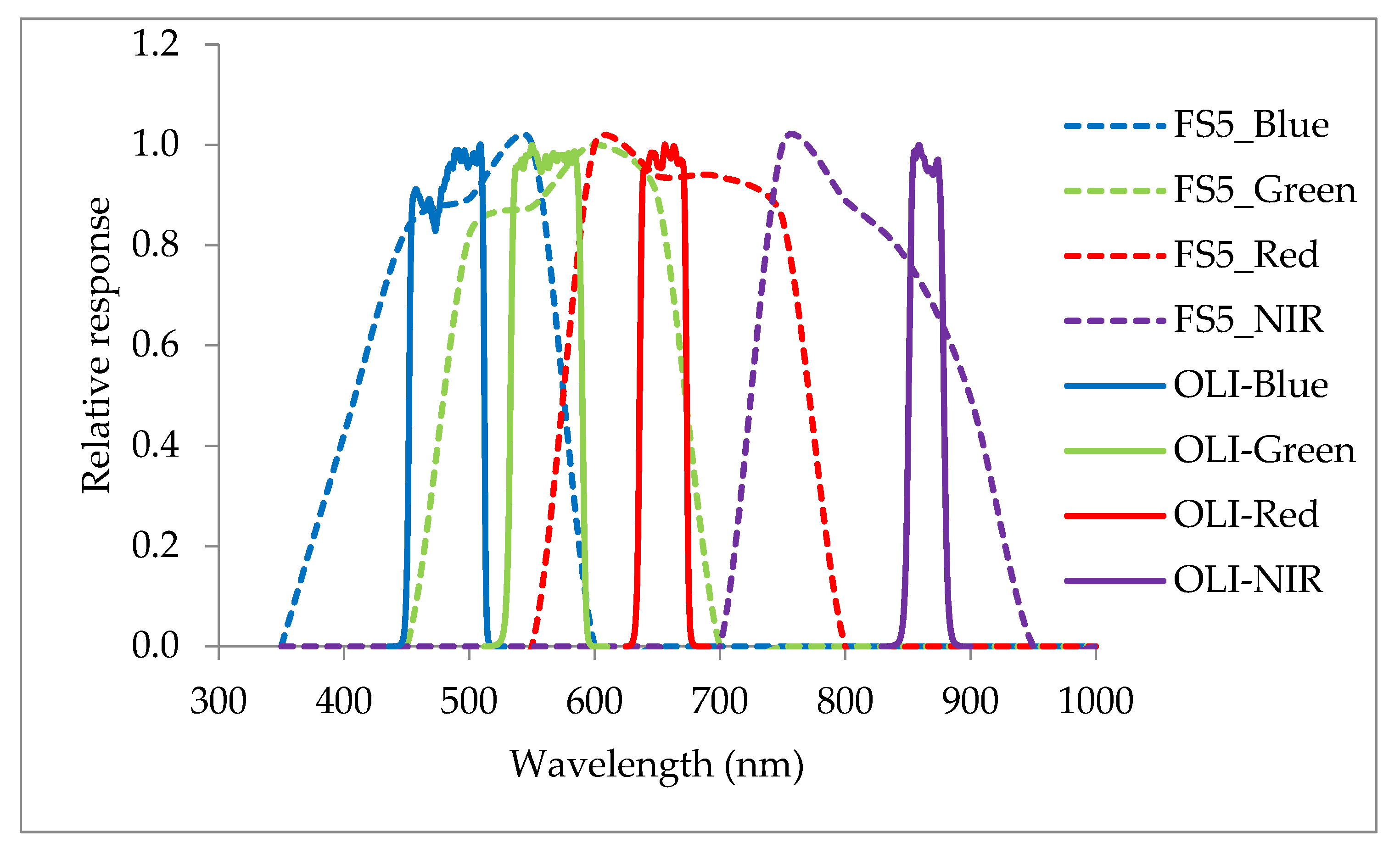
The FS5 provides 2 m resolution panchromatic and 4 m resolution multi-spectral images in a daily revisit orbit [45]. The NSPO provides FS5 with a digital number (DN) for four bands including blue, green, red, and near-infrared (NIR). FS5’s spectral bands, spatial resolution, gain, and offset values are shown in Table 1. A comparison of FS5 and OLI overlaying the visible and near-infrared parts of the spectrum is shown in Figure 2. The spectral response function of FS5 is provided by NSPO, and the respective spectral response functions documented for OLI are available at the Landsat Science website (https://landsat.gsfc.nasa.gov/wp-content/uploads/2013/06/Ball_BA_RSR.v1.1-1.xlsx) (accessed on 24 April 2021)
Due to the lack of matchup in situ measurement data points with FS5, the OLI image was selected as the reference data for cross-comparison and validation. There are many kinds of sensors that can be used as reference data. However, OLI data were selected instead of another satellite image because of the following reasons: Firstly, the OLI images with level-1 and level-2 are free for downloading from the United States Geological Survey (USGS) website (https://earthexplorer.usgs.gov/) (accessed on 12 April 2018). The OLI level-2 images already provide remote sensing reflectance, while OLI level-1 images can be used for computing remote sensing reflectance via many existing atmospheric corrections approaches. For example, the Fast Line-of-sight Atmospheric Analysis of Spectral Hypercubes (FLAASH) [46] model in the ENVI application, ACOLITE for aquatic application [47], and iCOR algorithm [16]. Secondly, the OLI-derived TSM image has been validated and discussed for Vietnamese coastal waters by using in situ measurement [22,37]. Lastly, the OLI images offer the scene with the time window between the FS5 and Landsat-8 OLI being <24 h.
To compare the satellite match-up dataset, we also evaluated the weather conditions and tidal characteristics at Ha Long Bay between FS5 and Landsat-8 OLI. The FS5 and Landsat-8 OLI satellites captured the scene at 10:30 local time on a sunny day with a partial cloud coverage of <10% and slight wind. Therefore, the weather assumed non-impact sediment characteristics under normal conditions. Weather conditions were evaluated based on historical global weather data (http://worldweatheronline.com) (accessed on 2 August 2021). Additionally, whether the tidal affected TSM characteristics were checked. Tidal characteristics in the study area are described in the tidal book published by the National Center for Hydro-Meteorological Forecasting, Vietnam Meteorological and Hydrological Administration (https://nchmf.gov.vn/) (accessed on 20 August 2021). The highest and lowest tidal levels were 3.4 m (05:27 local time) and 1.1 m (17:08 local time), respectively, on 10 November 2019, and 3.6 m (06:13 local time) and 0.9 m (18:41 local time), respectively, on 11 November 2019. Therefore, we assumed that weather conditions and sea surface characteristics were similar on 10–11 November 2019.
Based on the advantage of OLI data mentioned above, the FS5 satellite image was captured on 11 November 2019, and the Landsat-8 OLI image captured on 10 November 2019 was selected in a dataset for this study.
There were seven field surveys in different periods of time between 2011 and 2015 performed in Vietnam coastal waters. In situ data (n = 205 sample, with 67 samples related to Ha Long Bay) collected remote sensing reflectance (Rrs) and TSM as already described in [22,37]. It is noted that the in situ data were used to validate a TSM algorithm that can be applied to Landsat-8 OLI at Ha Long Bay with high correlation coefficients (R2 = 0.86).

2.3. Materials

We selected five types of land-cover objects as ground targets, and the number of samples is listed in Table 2. These objects were large, easily distinguishable, and observable across many geographical areas. The ground targets were divided into two categories: bright and dark. The bright targets included roofs, asphalt/concrete, and other materials (sand and soil) and accounted for most of the ground targets. The dark targets included water surfaces and vegetation [48] because these objects were already described according to the rapid atmospheric correction algorithm [15].
In this study, the dark targets included lake water, reservoirs, and vegetation. All the ground targets had a minimum size of 3 pixels × 3 pixels on the Landsat-8 OLI image, corresponding to 19 pixels × 19 pixels on the FS5 image. At least 26 objects were required for each ground target to ensure that the number of objects was sufficiently large and that the elevation was similar among these images. Finally, we obtained 160 samples (Figure 1) of the five land-cover objects and used them to perform linear regression analysis.

3. Methodology

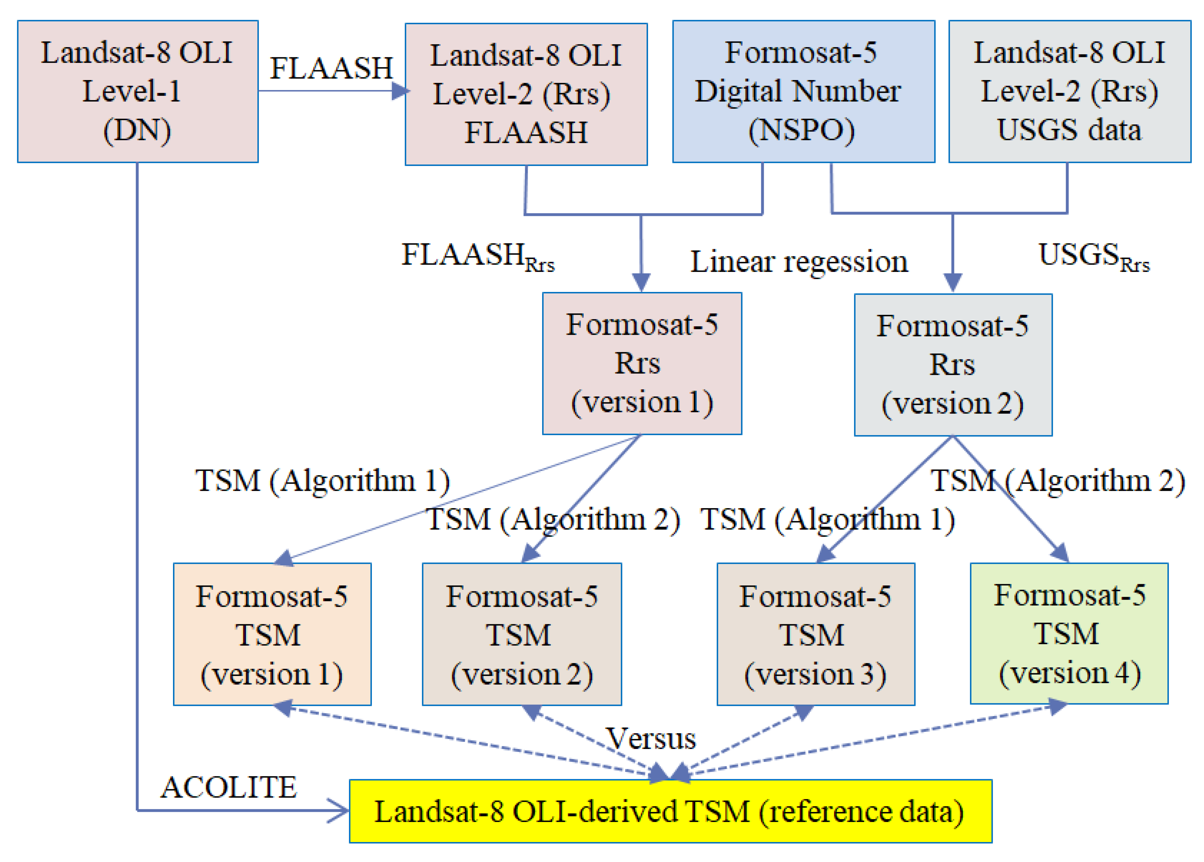
3.1. Data Processing

Data processing included three steps: converting a digital number (DN) to remote-sensing reflectance (Rrs) through linear regression, estimating the TSM concentration from the FS5 satellite image, and examining the accuracy. The flowchart of data processing is shown in Figure 3.
It is important to note that, since there are many atmospheric correction methods for aquatic applications related to Landsat-8 OLI images such as ACOLITE [47], C2RRC [49], iCOR [16], etc., we chose FLAASH in this study because we used ground targets as input data for linear regression. The FLAASH provides high stability and accuracy with ground targets. In addition, it is easy to set up using parameters such as sensor options, atmospheric model options, water retrieval options, etc., for local areas [46]. It is also easy to use in the ENVI application, and our research lab has good experience using this method. Finally, surface reflectance converted from FLAASH was used compared with USGS in order to avoid a biased selection for any one method. Therefore, we believe that FLAASH is the most suitable option for the purpose of this study.
The two top rows describe how the FS5’s DN value can be converted to Rrs through linear regression. Landsat-8 OLI level-2 reflectance was considered as reference data derived from level-1 by using the Fast Line-of-sight Atmospheric Analysis of Spectral Hypercubes (FLAASH) model in ENVI (RrsFLAASH) and downloaded from the United States Geological Survey (USGS) website (RrsUSGS). Linear regression was performed using the Landsat-8 OLI’s Rrs values of 160 ground targets (Figure 1) to convert the FS5’s DN value to the FS5’s Rrs value. This step resulted in two Rrs versions of FS5, namely FS5 Rrs version 1 and FS5 Rrs version 2. We compared the spectral profiles of the dark targets to determine the one favorable for coastal water applications.
The middle rows show the steps of TSM retrieved from FS5’s Rrs values. Two TSM algorithms (Algorithms 1 and 2 are described later in Section 3.3) with a red band from Landsat-8 OLI and the previous generation Formosat satellite images were used to compute TSM concentration images. The results provided four versions, named from 1 to 4, of the FS5 TSM images. Finally, as shown in the two last rows, we compared these FS5 TSM images with Landsat-8 OLI-derived TSM (reference data). Landsat-8 OLI-derived TSM was based on ACOLITE. ACOLITE is a generic processor developed by the Royal Belgian Institute of Natural Sciences (RBINS) for atmospheric correction and processing for coastal and inland water applications. It currently supports many sensors such as Landsat (5/7/8), Sentinel-2 (A/B), Sentinel-3 (A/B), PlanetScope, Pléiades, and WorldView. ACOLITE is provided for free, and the detail of ACOLITE can be found at link https://odnature.naturalsciences.be/remsem/software-and-data/acolite (accessed on 3 January 2022). We used ACOLITE because it provides an algorithm to retrieve TSM from remotely sensed data in all coastal and estuarine waters [21,38,47].
It is indicated that we use two different resources of OLI level-2 reflectance and two different TSM empirical algorithms. This is to avoid favoritism in the use of reference data related to surface reflections and the choice of TSM algorithms. Furthermore, the purpose of this data processing is to perform a comparison between two source data references and TSM algorithms.

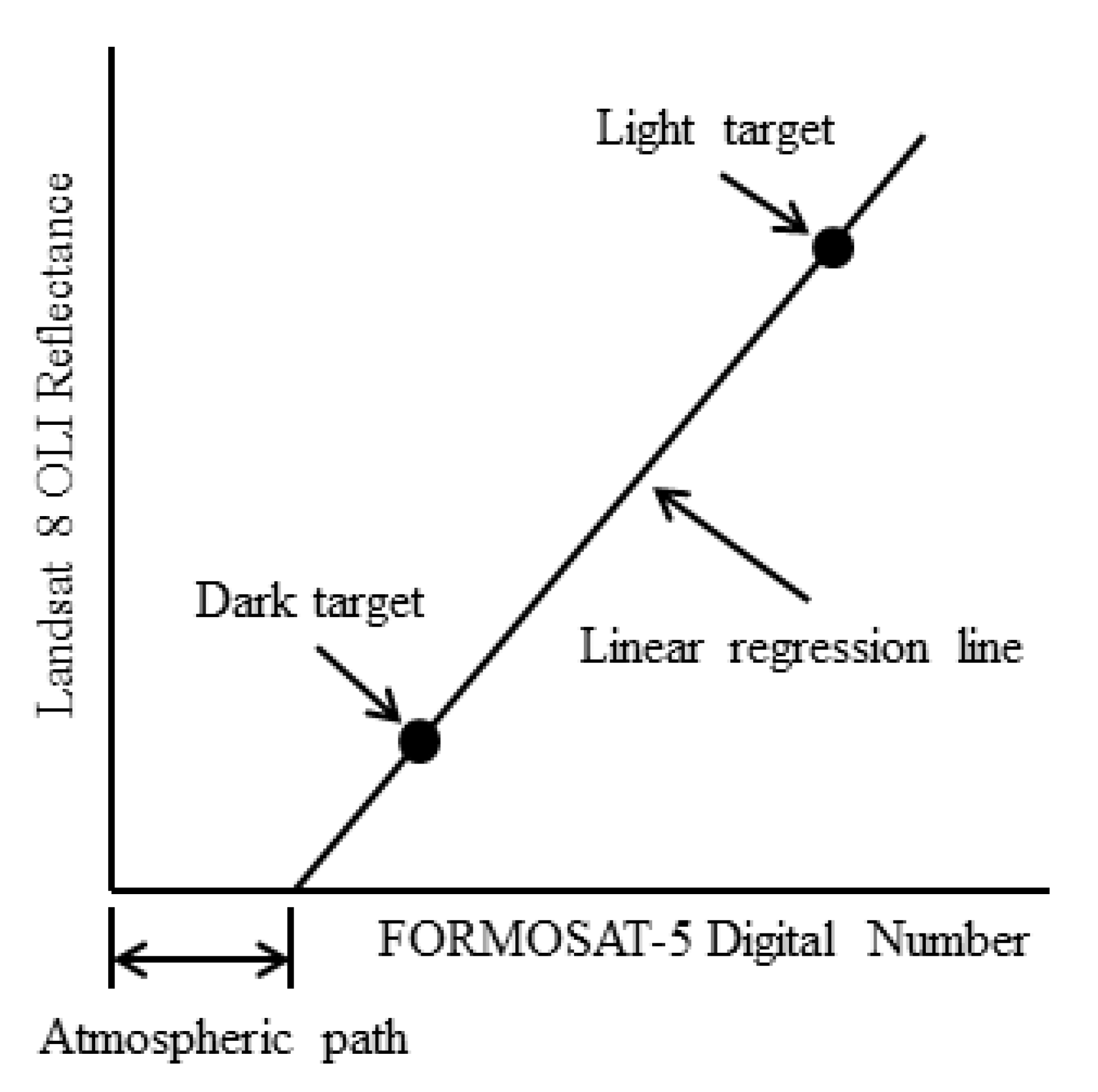
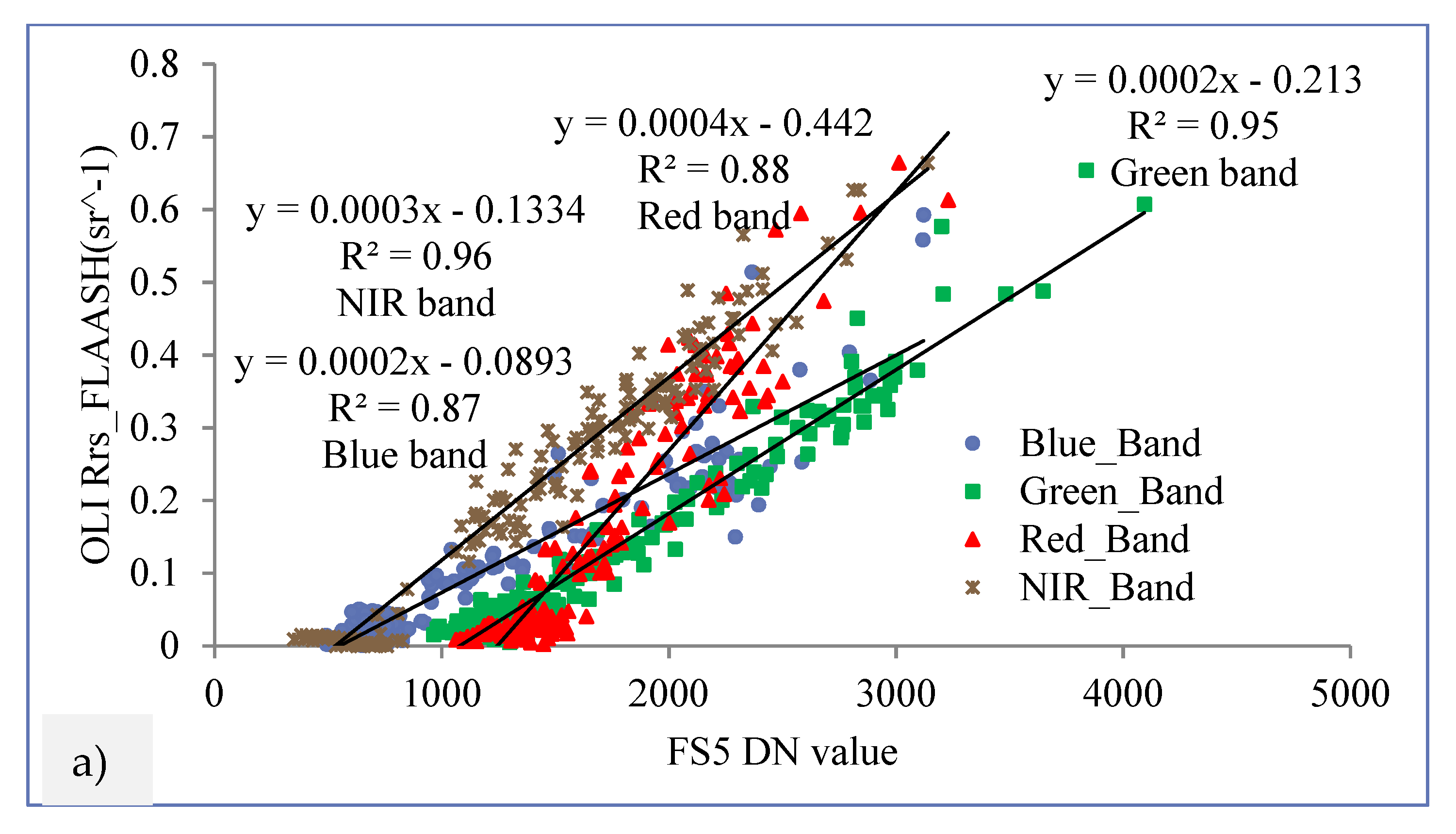
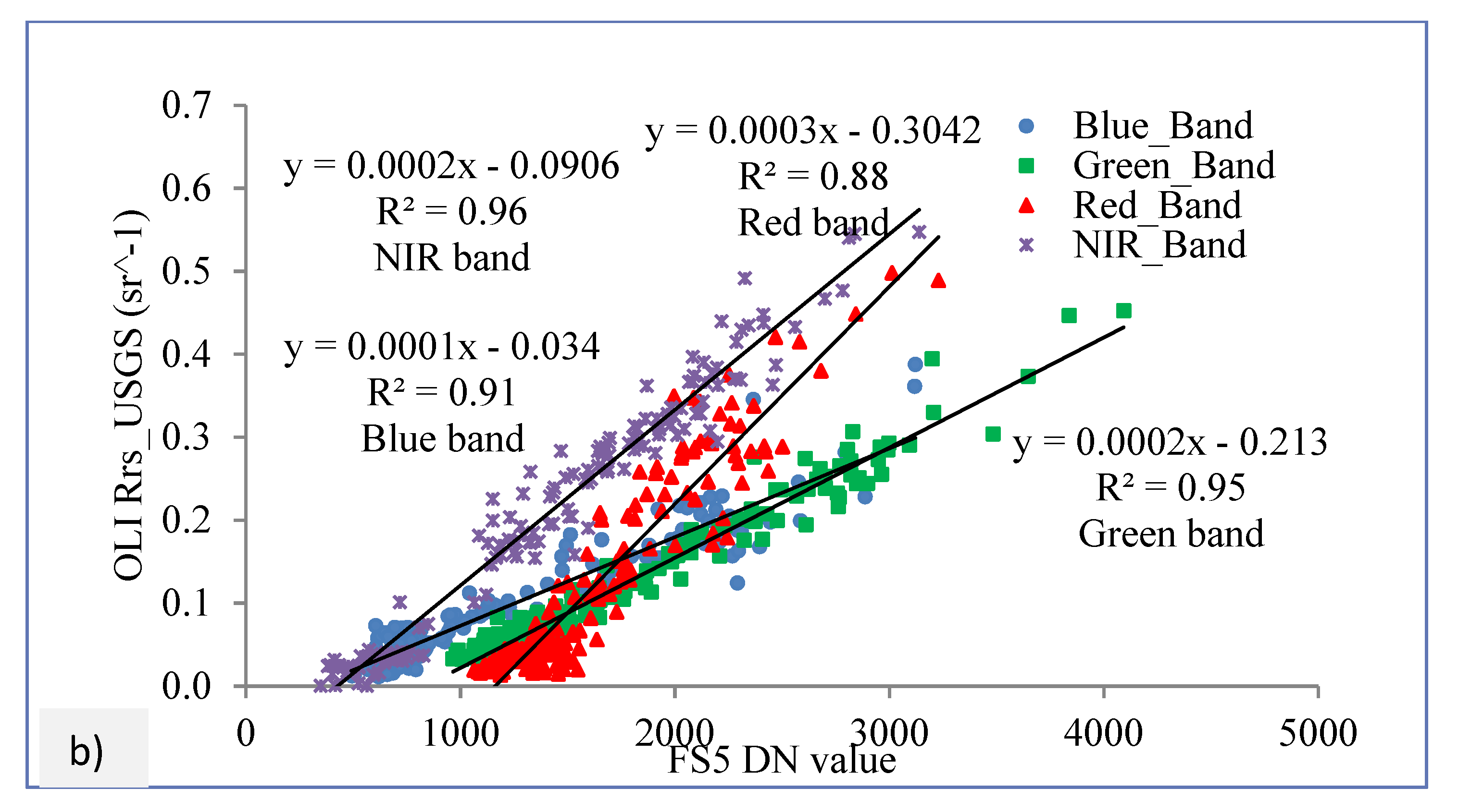
3.2. Convert the DN into Rrs

The actual surface reflectance in remotely sensed images taken by FS5 can be determined by removing specific weather-related atmospheric noise from a particular scene. The proposed method can easily remove atmospheric effects from satellite images through comparison between a pair of input and reference images of a scene [50,51,52]. However, the following conditions should be met:
  • The atmospheric effect should be constant across the entire image.
  • At least two consistent targets (bright and dark targets) should be easily identified in the scene.
  • The spectral profiles of ground targets should be similar between FS5 and Landsat-8 OLI when images are captured less than 24 h apart.
  • Linear regression should be performed to evaluate the relationship between the sensor’s radiance and surface reflectance.
Figure 4 shows how a linear regression model was used to convert the DN to Rrs. Linear regression is a common and effective method for removing the atmospheric effect from satellite images before evaluating coastal water areas. Linear regression is based on the assumption that a linear relationship exists between images’ DNs and ground measured reflectance for surfaces [17,19].
We used reflectance values derived from the Landsat-8 OLI for 160 samples of the five ground targets to perform linear regression analysis. These samples were divided into bright and dark targets. We assumed that when the time window between FS5 and Landsat-8 OLI images is <24 h, the reflectance of targets should remain invariant through time.
In this study, we used two Landsat-8 OLI level-2 sources obtained from the FLAASH model and downloaded them from the USGS website as reference data. Linear regression was performed on all four bands, namely blue, green, red, and NIR, between FS5 satellite images and reference data. To ensure the satisfactory conversion of a DN to Rrs, we set the smallest correlation coefficient for each band to be 0.85 (R2 ≥ 0.85). Furthermore, after the conversion process, the before and after spectral profiles of each sample were compared with Landsat-8 OLI results to assess the appropriateness of each approach.

3.3. TSM Concentration Algorithms

Two algorithms were adopted to calculate TSM concentrations by using the red band developed by Nechad et al. [38] and Richard et al. [24]. These two algorithms have reported correlation coefficients of 0.86 and 0.95, respectively
Nechad et al. developed a TSM algorithm that can be applied to diverse sensors such as Landsat-8 OLI and Sentinel-2 MSI [38]. This TSM algorithm (hereafter referred to as Algorithm 1) is based on the reflectance of the red band, and it is expressed as follows:
TSM = 384.11 ρ ω ( 655 ) 1 ρ ω ( 655 ) 0.1747 + 1.44
where ρ ω ( 655 ) = π R rs ( 655 ) .
Algorithm 1 had been checked and discussed for Vietnamese coastal waters; detail already described in [22,37]. By using in situ data (n = 205 samples, including 67 samples related to Ha Long Bay), Dat et al. had validated and indicated that the OLI-derived TSM image was processed to provide high accuracy with correlation coefficients of 0.86. The OLI image-derived TSM provides the accuracy with a low to moderate TSM concentration in a range of 3.33–15.25 mg/L.
The second TSM algorithm developed by Richard et al. (hereafter referred to as Algorithm 2) is related to the previous generation of FS5, FS2, as expressed in Equation (2) [24]:
TSM = 692.77 ×   R rs ( red ) + 3.7
It is necessary to say that Algorithm 2 was an algorithm designed for FS2. To apply Algorithm 2 to FS5 image, it must be cross-validated and discussed. Unfortunately, we did not have in situ measurement data for the validation of this algorithm. However, after reviewing and considering, we still chose Algorithm 2 for Ha Long Bay for the two following purposes: Firstly, this algorithm also uses the red band, which helps us to assess whether the red band can be used for TSM in Ha Long Bay. Secondly, we wanted to avoid unfairness in using only one algorithm to compute TSM concentration. It can help to make a comparison with the Algorithm 1.
We applied these two algorithms to red-band FS5’s Rrs images to estimate the TSM concentration. A total of four versions of TSM images were calculated and generated. Each of these TSM images was used to assess the accuracy and compare the spatial distribution of TSM concentrations with Landsat-8 OLI reference data (See Figure 3). The reference Landsat-8 OLI-derived TSM image was processed by using the ACOLITE application [47] with Nechad-OLI algorithm [38].

3.4. Accuracy Assessment

We used the TSM derived from the Landsat-8 OLI image as a reference to evaluate the accuracy of the TSM derived from the FS5 image. To account for differences in the resolution of the two images, we resampled FS5 from 4 m to 30 m resolution and subsequently used the root mean square error (RMSE) to determine the accuracy of the derived TSM. The purpose of resampling FS5 is to make an equal resolution with OLI (30 m) due to the different spatial resolutions of the two considered sensors. Furthermore, the resampled FS5 resolution process ensures it is possible to compare with OLI based on the histogram and the scatter plot with the same number of pixels.
The RMSE between the two TSM images was computed as follows:
RMSE = [ ( TSM FS 5   TSM OLI ) 2 N ] 0.5
where TSM FS 5 and TSM OLI are TSM derived from FS5 and Landsat-8 OLI, respectively, and N represents the number of samples.
Furthermore, a histogram was used to compare the distribution of TSM concentrations between FS5-derived TSM and Landsat-8 OLI-derived TSM.

4. Results

4.1. FS5 Rrs Retrieval

Figure 5 presents the results of a linear regression performed on the four bands of images derived from both FS5 and Landsat-8 OLI for a total of 160 ground objects. Figure 5a shows the linear regression generated using FS5’s DN and Landsat-8 OLI’s Rrs derived from the FLAASH model, and Figure 5b shows linear regression generated using FS5’s DN and Landsat-8 OLI’s Rrs downloaded from the USGS website.
As shown in Figure 5a, the largest correlation coefficient was obtained for the NIR band (R2 = 0.96), which was followed by the green band (R2 = 0.95), whereas the smallest correlation coefficient was obtained for the blue band (R2 = 0.87). Meanwhile, as presented in Figure 5b, the largest correlation coefficient was also observed for the NIR band (R2 = 0.96), which was also followed by the green band (R2 = 0.95), whereas the smallest correlation coefficient was noted for the red band (R2 = 0.88). Both approaches provided an R2 value of >0.85, indicating their satisfactory performance in converting the DN to Rrs. The results revealed that Landsat-8 OLI level-2 from FLAASH and USGS sources can be employed to compute the same values of Rrs for FS5 images based on linear regression.

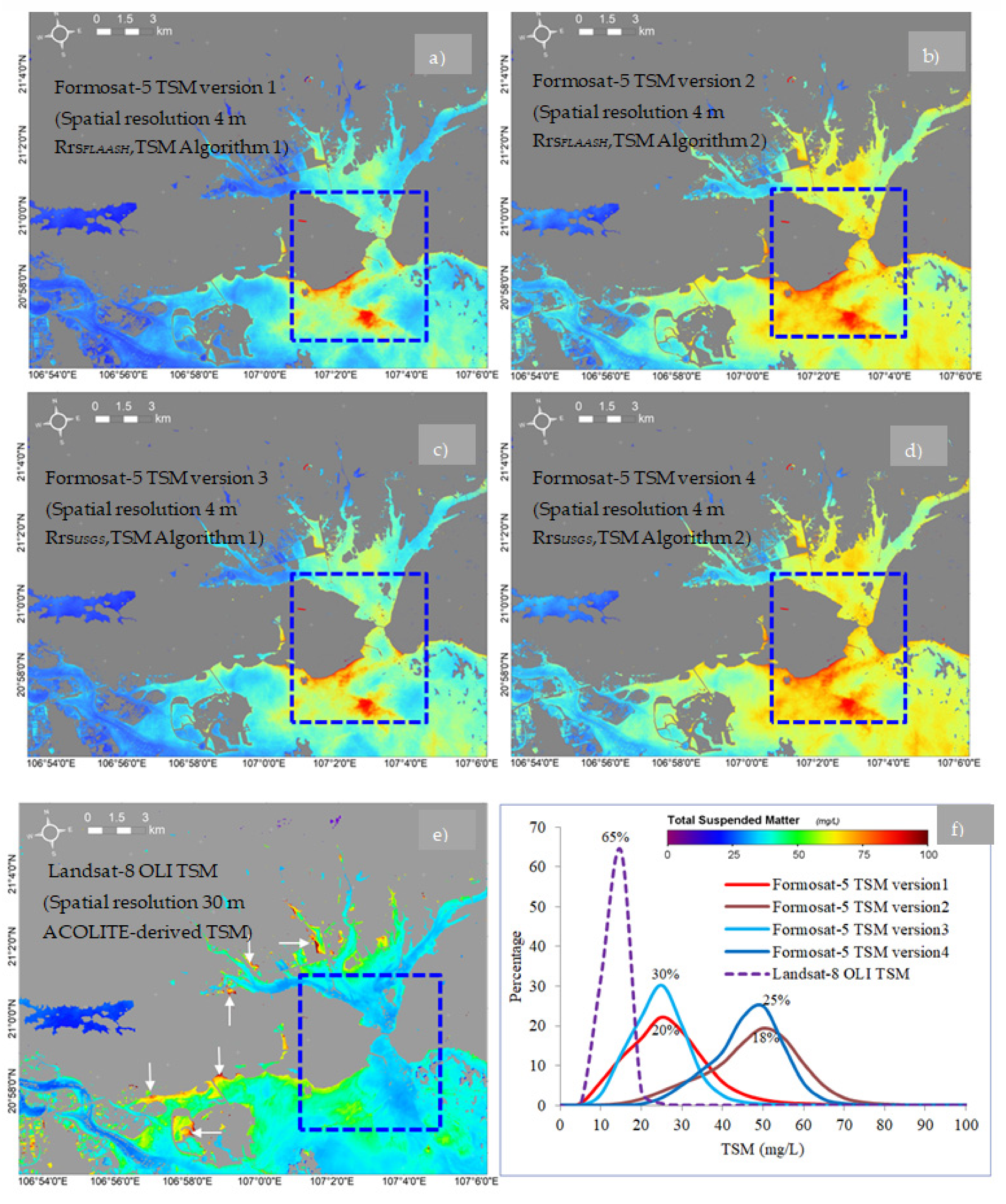
4.2. FS5 Image-Derived TSM for Ha Long Bay, Vietnam

Figure 6 shows the FS5 image-derived TSM for Ha Long Bay, Vietnam, by using the two algorithms. A significant difference was observed between the FS5-derived 4 m TSM image and the Lansat-8 OLI-derived 30 m TSM image related to the spatial distribution and concentration of TSM.
Figure 6e shows the 30 m TSM image derived from Landsat-8 OLI by using the ACOLITE application. TSM with a high concentration was distributed outside of the blue rectangle. High TSM values ranging from 75 to 100 mg/L were distributed in coastline areas (denoted by arrows), whereas low TSM values ranging from 25 to 50 mg/L were observed far from the coastline. The histogram of the Landsat-8 OLI-derived TSM indicated that TSM ranged from 5 to 25 mg/L, with a peak at 15 mg/L accounting for 65% of the total TSM (Figure 6f).
Figure 6a–d show the 4 m TSM image derived from FS5. Compare these images to that in Figure 6e, where the FS5-derived TSM with high values was distributed inside the blue rectangle. As shown in Figure 6a–e, the position of TSM with the highest concentration differed between FS5 and OLI images. Therefore, additional analysis and discussion regarding this topic are required in the future.
This can be compared with Figure 6a,c,e to show a significant difference in the spatial distribution of TSM with both the highest and lowest values. The histogram shown in Figure 6a indicates that the FS5-derived TSM version 1 image was dominated by the TSM ranging from 5 to 60 mg/L, with a peak at 25 mg/L (accounting for approximately 20%). The histogram shown in Figure 6c indicates that the FS5-derived TSM version 3 image was dominated by TSM ranging from 5 to 50 mg/L, with a peak at 20 mg/L (accounting for approximately 30%). These results revealed a significant difference between FS5-derived TSM using TSM Algorithm 1 and Landsat-8 OLI-derived TSM.
A slight difference was noted between both the highest and lowest values of TSM (Figure 6b,d). The histogram shown in Figure 6b indicates that the FS5-derived TSM version 2 image was dominated by TSM ranging from 10 to 80 mg/L, with a peak at 50 mg/L (accounting for approximately 18%). Moreover, the histogram shown in Figure 6d indicates that the FS5-derived TSM version 4 image was dominated by TSM ranging from 15 to 70 mg/L, with a peak at 50 mg/L (accounting for approximately 25%). These results revealed a significant difference between FS5-derived TSM determined using TSM Algorithm 2 and Landsat-8 OLI-derived TSM. It also indicated that, compared with Landsat-8 OLI-derived TSM, the histogram of TSM derived from Algorithm 1 was more reliable than that from Algorithm 2.
On the basis of the spatial distribution of TSM observed in Ha Long Bay and the TSM concentration range from histograms, we suggest using the TSM version 1 algorithm to estimate TSM applications in Ha Long Bay. However, although a difference was noted between the FS5-derived 4 m TSM image and Landsat-8 OLI-derived 30 m TSM image, all FS5-derived images should be considered until in situ measurement data are collected to validate all results. Furthermore, potential factors contributing to this difference should be investigated in the future.

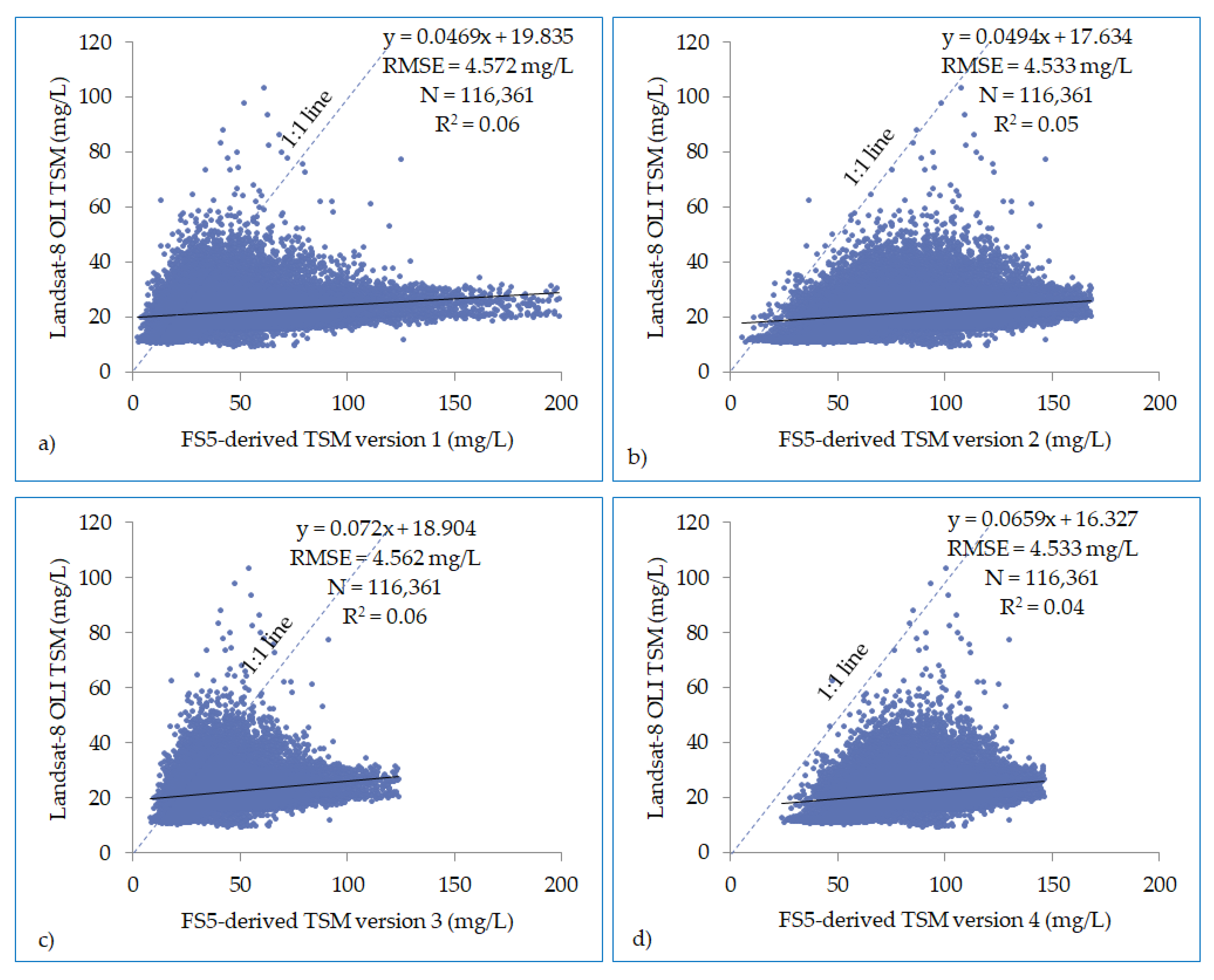
4.3. Comparing the Accuracy of FS5-Derived TSM and Landsat-8 OLI-Derived TSM

We used the RMSE to evaluate the accuracy of the FS5 image-derived TSM compared with the Landsat-8 OLI image-derived TSM (Figure 6e). For this purpose, we resampled the FS5’s images to a spatial resolution of 30 m.
Figure 7 compares the accuracy between FS5-derived TSM and Landsat-8 OLI-derived TSM. Overall, TSM results derived from FS5 images have higher concentrations than those from OLI’s. The highest TSM value up to 200 mL/L belongs to the FS5-derived TSM version 1, which was followed by the FS5-derived TSM version 2 with the highest TSM value of about 170 mL/L. Meanwhile, the highest TSM value of about 120 mL/L belongs to the FS5-derived TSM version 4. The results from scatter plots indicated that FS5-derived TSM version 3 and FS5-derived TSM version 4 are comparable with Landsat-8 OLI-derived TSM. This means that RrsUSGS should be considered instead of RrsFLAASH to retrieve TSM in Ha Long Bay.
Table 3 shows the findings of the comparison of RMSE between FS5- and OLI-derived TSM images at 30 m resolution. The application of the TSM version 2 algorithm to both the RrsFLAASH and RrsUSGS images provided RMSE values of 4.533 mg/L, respectively. Moreover, the application of the TSM version 1 algorithm to both the RrsFLAASH and RrsUSGS images provided RMSE values of 4.572 and 4.562 mg/L, respectively. The results indicated that the RrsUSGS provided a lower RMSE value than RrsFLAASH.
According to the spatial distribution of FS5-derived TSM images, the histogram, the scatter plots, and RMSE results, the TSM Algorithm 1 and RrsUSGS should be considered for estimating TSM applications in Ha Long Bay.
It is notable that the Algorithm 1 with the red band we used to estimate the TSM concentration is developed to OLI with a spatial resolution of 30 m. Therefore, an independent algorithm with a single band or multiple bands should be developed to estimate the TSM concentration for FS5 images with the spatial resolution of 4 m. Moreover, factors contributing to differences in the spatial distribution and concentration between the FS5-derived 4 m TSM image and the Landsat-8 OLI-derived 30 m TSM image have not yet been fully investigated and thus should be examined in future studies.

5. Discussion

Several problems should be resolved to improve the application of FS5 for coastal water regions, including the removal of the atmospheric effect, using the algorithm to estimate TSM concentrations, and accurately assessing the spatial distribution of sediment concentrations.
In this study, we proposed using linear regression to convert a DN to Rrs to remove the atmospheric effect. This method yielded favorable results and is easy to use when a matching dataset is available between FS5 and LS8. The advantage of this approach is that the scene belonging to both FS5 and Landsat-8 OLI is captured simultaneously within 24 h. Therefore, the form of the spectral profile at ground targets is assumed to be unchanged. Previous studies have frequently used spectrophotometric instruments in the field to collect reference data. Therefore, we believe that an empirical approach can be used as an alternative solution to unsuitable satellite images. This should be implemented by independent studies on atmospheric correction for FS5 in the future.
Studies should examine which factors contribute to the difference between FS5-derived TSM and OLI-derived TSM. Because no field in situ measurements in the study area were collected that matched FS5 images, we used two algorithms developed for OLI and FS2 based on the red band to estimate TSM concentrations [3,18]. The results revealed that the concentration of FS5-derived TSM tended to be higher than that of OLI-derived TSM. In particular, OLI-derived TSM concentrations mainly ranged from 5 to 25 mg/L, whereas FS5-derived TSM concentrations ranged from 5 to 60 mg/L (Algorithm 1) and 10–80 mg/L (Algorithm 2 and Figure 6f). This difference may be because we considered two different algorithms with only the red band. Therefore, a TSM-independent algorithm for FS5 based on in situ measurement data should be developed in the future. Furthermore, not only a single band but also multiple bands should be considered because it is a necessity for a new sensor such as FS5.
OLI images processed to estimate TSM by using ACOLITE can be applied to all estuaries and coastal areas [21], including coastal Vietnam [22]. The accuracy of TSM results ranged from 0 to 20 mg/L when the TSM concentration ranged from 0 to 1000 mg/L. A comparison of TSM concentrations between FS5-derived TSM and OLI-derived TSM based on RMSE showed that the lowest RMSE was 4.533 mg/L (Algorithm 2) and 4.562 (Algorithm 1). Although the RMSE is acceptable because OLI image-derived TSM provides accuracy with a range of 3.33–15.25 mg/L [21], it can be further improved if field measurement data are available to validate this result. Therefore, the accuracy of the estimation of the FS5-derived TSM concentration based on algorithms should be improved in future studies.
This study only proposes using FS5 for estimating TSM in the north of Vietnam. We believe after removing the effect of atmospheric on FS5’s images and overpassing the limitation of lack data of in situ measurement, FS5 could be useful for estimating many applications related to the aquatic application in both inland and coastal water such as monitoring sediment at river mouths and estuary systems, water quality indexes in reservoirs, and seasonal variations in shallow water. For example, the advantage in temporal of FS5 can be used for monitoring the spatial distribution of TSM before and after typhoons. The high spatial resolution can monitor characteristics of TSM in seasonal variation of sediment and perform comparisons between dry and wet seasons. For this purpose, potential applications of FS5 should be further explored in future studies to overcome the limitations mentioned in this study. At the same time, diversifying solutions using FS5 satellite images in real applications should be considered not only in Vietnamese coastal waters but also everywhere covered by FS5’s footprint.

6. Conclusions

This is the first study to propose the use of high-resolution FS5 satellite images to estimate TSM concentrations in a coastal water region. Linear regression was used to remove atmospheric effects from an FS5 image based on the surface reflectance for 160 samples of ground targets. Using Landsat-8 OLI level-2 sources as reference data, we converted the FS5’s DN value to the Rrs value for four bands with an R2 of 0.88–0.96. The results indicated that Landsat-8 OLI level-2 derived from both FLAASH and USGS sources can be used to compute Rrs for FS5 images based on linear regression.
According to a comparison of histogram and RMSE results, we indicated that RrsUSGS and the TSM version 1 algorithm developed by Nechad et al. should be selected for FS5 images estimating TSM concentrations at Ha Long Bay, Vietnam. Moreover, we also suggest that an independent algorithm for estimating TSM concentration for FS5 images with multiple bands rather than a single band should be considered. The results indicated a marked difference in the spatial distribution of TSM between the FS5 4 m image and Landsat-8 OLI 30 m image. Therefore, factors affecting the spatial distribution and concentration of FS5’s TSM image should be also investigated in the future.
FS5 images can reliably be applied for evaluating the optical characteristics of coastal waters belonging to Ha Long Bay. The high spatiotemporal resolution of FS5 images after the removal of atmospheric effects can be useful for estimating TSM in coastal water regions.

Author Contributions

Conceptualization, C.-K.W.; Data curation, P.-M.C.; Formal analysis, P.-M.C.; Investigation, P.-M.C.; Methodology, P.-M.C. and C.-K.W.; Project administration, C.-K.W.; Software, P.-M.C.; Supervision, C.-K.W.; Validation, P.-M.C.; Visualization, P.-M.C.; Writing an original draft, P.-M.C.; Writing—review and editing, C.-K.W. All authors have read and agreed to the published version of the manuscript.

Funding

This research received no external funding.

Institutional Review Board Statement

Not applicable.

Informed Consent Statement

Not applicable.

Data Availability Statement

The data that support the findings of this study are available from the corresponding author upon reasonable request.

Acknowledgments

The authors would like to thank the National Space Organization (NSPO) of Taiwan for providing FS5 level-1B satellite images. The authors also thank the United States Geological Survey (USGS) for providing Landsat-8 OLI level-1 and level-2. Lastly, the authors thank the Royal Belgian Institute of Natural Sciences (RBINS) for free sharing ACOLITE application.

Conflicts of Interest

The authors declare no conflict of interest.

References

  1. Snelgrove, P.V.R.; Henry Blackburn, T.; Hutchings, P.A.; Alongi, D.M.; Frederick Grassle, J.; Hummel, H.; King, G.; Koike, I.; Lambshead, P.J.D.; Ramsing, N.B.; et al. The importance of marine sediment biodiversity in ecosystem processes. Ambio 1997, 26, 578–583. [Google Scholar] [CrossRef]
  2. Chen, S.; Huang, W.; Wang, H.; Li, D. Remote sensing assessment of sediment re-suspension during Hurricane Frances in Apalachicola Bay, USA. Remote Sens. Environ. 2009, 113, 2670–2681. [Google Scholar] [CrossRef]
  3. Casal, G.; Harris, P.; Monteys, X.; Hedley, J.; Cahalane, C.; Casal, G.; Harris, P.; Monteys, X.; Hedley, J.; Cahalane, C.; et al. Understanding satellite-derived bathymetry using Sentinel 2 imagery and spatial prediction models. GIScience Remote Sens. 2019, 57, 271–286. [Google Scholar] [CrossRef]
  4. Volpe, V.; Silvestri, S.; Marani, M. Remote sensing retrieval of suspended sediment concentration in shallow waters. Remote Sens. Environ. 2011, 115, 44–54. [Google Scholar] [CrossRef]
  5. Malenovský, Z.; Rott, H.; Cihlar, J.; Schaepman, M.E.; García-Santos, G.; Fernandes, R.; Berger, M. Sentinels for science: Potential of Sentinel-1, -2, and -3 missions for scientific observations of ocean, cryosphere, and land. Remote Sens. Environ. 2012, 120, 91–101. [Google Scholar] [CrossRef]
  6. Ody, A.; Doxaran, D.; Vanhellemont, Q.; Nechad, B.; Novoa, S.; Many, G.; Bourrin, F.; Verney, R.; Pairaud, I.; Gentili, B. Potential of high spatial and temporal ocean color satellite data to study the dynamics of suspended particles in a micro-tidal river plume. Remote Sens. 2016, 8, 245. [Google Scholar] [CrossRef] [Green Version]
  7. Yuei-An, L.; Kar, S.K.; Chang, L. Use of high-resolution formosat-2 satellite images for post-earthquake disaster assessment: A study following the 12 may 2008 Wenchuan Earthquake. Int. J. Remote Sens. 2010, 31, 3355–3368. [Google Scholar] [CrossRef]
  8. Chen, K.S.; Wu, A.M.; Chern, J.S.; Chen, L.C.; Chang, W.Y. FORMOSAT-2 mission: Current status and contributions to earth observations. Proc. IEEE 2010, 98, 878–891. [Google Scholar] [CrossRef]
  9. Courault, D.; Bsaibes, A.; Kpemlie, E.; Hadria, R.; Hagolle, O.; Marloie, O.; Hanocq, J.F.; Olioso, A.; Bertrand, N.; Desfonds, V. Assessing the potentialities of FORMOSAT-2 data for water and crop monitoring at small regional scale in South-Eastern France. Sensors 2008, 8, 3460–3481. [Google Scholar] [CrossRef] [Green Version]
  10. Yang, K.-J.; Chang, C.-H.; Liu, C.-C.; Yao, -S.C. 4Integration of MODIS and Formosat-2 Imagery for the Development of a Reliable and High-Tempospatial-Resolution Total Suspended Matter Concentration Retrieval Model: Case Study in Goaping River Mouth. J. Photogramm. Remote Sens. 2013, 17, 53–65. [Google Scholar]
  11. Chung, H.W.; Liu, C.C.; Chiu, Y.S.; Liu, J.T. Spatiotemporal variation of Gaoping River plume observed by Formosat-2 high resolution imagery. J. Mar. Syst. 2014, 132, 28–37. [Google Scholar] [CrossRef]
  12. Chang, C.H.; Liu, C.C.; Wen, C.G.; Cheng, I.F.; Tam, C.K.; Huang, C.S. Monitoring reservoir water quality with Formosat-2 high spatiotemporal imagery. J. Environ. Monit. 2009, 11, 1982–1992. [Google Scholar] [CrossRef] [PubMed]
  13. Mograne, M.; Jamet, C.; Loisel, H.; Vantrepotte, V.; Mériaux, X.; Cauvin, A. Evaluation of Five Atmospheric Correction Algorithms over French Optically-Complex Waters for the Sentinel-3A OLCI Ocean Color Sensor. Remote Sens. 2019, 11, 668. [Google Scholar] [CrossRef] [Green Version]
  14. He, Q.; Chen, C. A new approach for atmospheric correction of MODIS imagery in turbid coastal waters: A case study for the Pearl River Estuary. Remote Sens. Lett. 2014, 5, 249–257. [Google Scholar] [CrossRef]
  15. Wang, D.; Ma, R.; Xue, K.; Loiselle, S.A. The assessment of landsat-8 OLI atmospheric correction algorithms for inland waters. Remote Sens. 2019, 11, 169. [Google Scholar] [CrossRef] [Green Version]
  16. DeKeukelaere, L.; Sterckx, S.; Adriaensen, S.; Knaeps, E.; Reusen, I.; Giardino, C.; Bresciani, M.; Hunter, P.; Neil, C.; Van derZande, D.; et al. Atmospheric correction of Landsat-8/OLI and Sentinel-2/MSI data using iCOR algorithm: Validation for coastal and inland waters. Eur. J. Remote Sens. 2018, 51, 525–542. [Google Scholar] [CrossRef] [Green Version]
  17. Ariza, A.; Robredo Irizar, M.; Bayer, S. Empirical line model for the atmospheric correction of sentinel-2A MSI images in the Caribbean Islands. Eur. J. Remote Sens. 2018, 51, 765–776. [Google Scholar] [CrossRef]
  18. Karpouzli, E.; Malthus, T. The empirical line method for the atmospheric correction of IKONOS imagery. Int. J. Remote Sens. 2003, 24, 1143–1150. [Google Scholar] [CrossRef]
  19. Pompilio, L.; Marinangeli, L.; Amitrano, L.; Pacci, G.; D’Andrea, S.; Iacullo, S.; Monaco, E. Application of the empirical line method (ELM) to calibrate the airborne Daedalus-CZCS scanner. Eur. J. Remote Sens. 2018, 51, 33–46. [Google Scholar] [CrossRef] [Green Version]
  20. Moran, M.S.; Bryant, R.; Thome, K.; Ni, W.; Nouvellon, Y.; Gonzalez-Dugo, M.P.; Qi, J.; Clarke, T.R. A refined empirical line approach for reflectance factor retrieval from Landsat-5 TM and Landsat-7 ETM+. Remote Sens. Environ. 2001, 78, 71–82. [Google Scholar] [CrossRef]
  21. Dogliotti, A.I.; Ruddick, K.G.; Nechad, B.; Doxaran, D.; Knaeps, E. A single algorithm to retrieve turbidity from remotely-sensed data in all coastal and estuarine waters. Remote Sens. Environ. 2015, 156, 157–168. [Google Scholar] [CrossRef] [Green Version]
  22. Ngoc, D.D.; Loisel, H.; Vantrepotte, V.; Xuan, H.C.; Minh, N.N.; Verpoorter, C.; Meriaux, X.; Minh, H.P.T.; Thi, H.L.; Hong, H.L.V.; et al. A simple empirical band-ratio algorithm to assess suspended particulate matter from remote sensing over coastal and inland waters of vietnam: Application to the VNREDSat-1/NAOMI sensor. Water 2020, 12, 2636. [Google Scholar] [CrossRef]
  23. Miller, R.L.; McKee, B.A. Using MODIS Terra 250 m imagery to map concentrations of total suspended matter in coastal waters. Remote Sens. Environ. 2004, 93, 259–266. [Google Scholar] [CrossRef]
  24. Miller, R.L.; Liu, C.C.; Buonassissi, C.J.; Wu, A.M. A multi-sensor approach to examining the distribution of total suspended matter (TSM) in the Albemarle-Pamlico Estuarine System, NC, USA. Remote Sens. 2011, 3, 962–974. [Google Scholar] [CrossRef] [Green Version]
  25. Balasubramanian, S.V.; Pahlevan, N.; Smith, B.; Binding, C.; Schalles, J.; Loisel, H.; Gurlin, D.; Greb, S.; Alikas, K.; Randla, M.; et al. Robust algorithm for estimating total suspended solids (TSS) in inland and nearshore coastal waters. Remote Sens. Environ. 2020, 246, 111768. [Google Scholar] [CrossRef]
  26. Liu, G.; Li, L.; Song, K.; Li, Y.; Lyu, H.; Wen, Z.; Fang, C.; Bi, S.; Sun, X.; Wang, Z.; et al. An OLCI-based algorithm for semi-empirically partitioning absorption coefficient and estimating chlorophyll a concentration in various turbid case-2 waters. Remote Sens. Environ. 2020, 239, 111648. [Google Scholar] [CrossRef]
  27. Huang, C.C.; Chang, M.J.; Lin, G.F.; Wu, M.C.; Wang, P.H. Real-time forecasting of suspended sediment concentrations reservoirs by the optimal integration of multiple machine learning techniques. J. Hydrol. Reg. Stud. 2021, 34, 100804. [Google Scholar] [CrossRef]
  28. Li, Y.; Xu, X.; Zheng, B. Satellite views of cross-strait sediment transport in the Taiwan Strait driven by Typhoon Morakot (2009). Cont. Shelf Res. 2018, 166, 54–64. [Google Scholar] [CrossRef]
  29. Yang, G.; Wang, X.H.; Ritchie, E.A.; Qiao, L.; Li, G.; Cheng, Z. Using 250-M surface reflectance MODIS Aqua/Terra product to estimate turbidity in a macro-tidal harbour: Darwin Harbour, Australia. Remote Sens. 2018, 10, 997. [Google Scholar] [CrossRef] [Green Version]
  30. Qiu, Z.; Xiao, C.; Perrie, W.; Sun, D.; Wang, S.; Shen, H.; Yang, D.; He, Y. Using Landsat 8 data to estimate suspended particulate matter in the Yellow River estuary. J. Geophys. Res. Ocean. 2017, 122, 276–290. [Google Scholar] [CrossRef]
  31. Qiu, Z. A simple optical model to estimate suspended particulate matter in Yellow River Estuary. Opt. Express 2013, 21, 27891. [Google Scholar] [CrossRef] [PubMed]
  32. Vanhellemont, Q.; Ruddick, K. Atmospheric correction of Sentinel-3/OLCI data for mapping of suspended particulate matter and chlorophyll-a concentration in Belgian turbid coastal waters. Remote Sens. Environ. 2021, 256, 112284. [Google Scholar] [CrossRef]
  33. Wang, H.; Wang, J.; Cui, Y.; Yan, S. Consistency of suspended particulate matter concentration in turbid water retrieved from sentinel-2 msi and landsat-8 oli sensors. Sensors 2021, 21, 1662. [Google Scholar] [CrossRef] [PubMed]
  34. Molkov, A.A.; Fedorov, S.V.; Pelevin, V.V.; Korchemkina, E.N. Regional models for high-resolution retrieval of chlorophyll a and TSM concentrations in the Gorky Reservoir by Sentinel-2 imagery. Remote Sens. 2019, 11, 1215. [Google Scholar] [CrossRef] [Green Version]
  35. Nazirova, K.; Alferyeva, Y.; Lavrova, O.; Shur, Y.; Soloviev, D.; Bocharova, T.; Strochkov, A. Comparison of in situ and remote-sensing methods to determine turbidity and concentration of suspended matter in the estuary zone of the mzymta river, black sea. Remote Sens. 2021, 13, 143. [Google Scholar] [CrossRef]
  36. Aswathy, T.S.; Achu, A.L.; Francis, S.; Gopinath, G.; Joseph, S.; Surendran, U.; Sunil, P.S. Assessment of water quality in a tropical ramsar wetland of southern India in the wake of COVID-19. Remote Sens. Appl. Soc. Environ. 2021, 23, 100604. [Google Scholar] [CrossRef]
  37. Loisel, H.; Vantrepotte, V.; Ouillon, S.; Ngoc, D.D.; Herrmann, M.; Tran, V.; Mériaux, X.; Dessailly, D.; Jamet, C.; Duhaut, T.; et al. Assessment and analysis of the chlorophyll-a concentration variability over the Vietnamese coastal waters from the MERIS ocean color sensor (2002–2012). Remote Sens. Environ. 2017, 190, 217–232. [Google Scholar] [CrossRef]
  38. Nechad, B.; Ruddick, K.G.; Park, Y. Calibration and validation of a generic multisensor algorithm for mapping of total suspended matter in turbid waters. Remote Sens. Environ. 2010, 114, 854–866. [Google Scholar] [CrossRef]
  39. Le, T.A. Situation Analysis of the Water Quality of Ha Long Bay, Quang Ninh Province, Vietnam: A Social Study from Tourism Businesses’ Perspectives; IUCN: Gland, Switzerland, 2015. [Google Scholar]
  40. Republic, S.; Ninh, Q.; People, P. The Project for Environmental Protection in Halong Bay. 2013, Volume 2. Available online: http://open_jicareport.jica.go.jp/pdf/1000021863_01.pdf (accessed on 20 June 2021).
  41. Nguyen, M.H.; Ouillon, S.; Vu, D.V. Seasonal variation of suspended sediment and its relationship with turbidity in Cam-Nam Trieu estuary, Hai Phong (Vietnam). Tạp chí Khoa học và Công nghệ Biển 2021, 21, 271–282. [Google Scholar] [CrossRef]
  42. Vinh, V.D.; Ouillon, S.; Thanh, T.D.; Chu, L.V. Impact of the Hoa Binh dam (Vietnam) on water and sediment budgets in the Red River basin and delta. Hydrol. Earth Syst. Sci. 2014, 18, 3987–4005. [Google Scholar] [CrossRef] [Green Version]
  43. Vinh, V.D.; Uu, D. Vanthe Influence of Wind and Oceanographic Factors on Characteristics of Suspended Sediment Transport in Bach Dang Estuary. Tạp chí Khoa học và Công nghệ Biển 2013, 13, 216–226. [Google Scholar] [CrossRef]
  44. Tu, T.A. Đánh Giá Đặc Trưng Trầm Tích Lơ Lửng Khu Vực Cửa Sông Ven Biển Hải Phòng; ĐHKHTN: Ha Noi, Vietnam, 2012. [Google Scholar]
  45. Lin, T.H.; Chang, J.C.; Hsu, K.H.; Lee, Y.S.; Zeng, S.K.; Liu, G.R.; Tsai, F.A.; Chan, H.P. Radiometric variations of On-Orbit FORMOSAT-5 RSI from vicarious and cross-calibration measurements. Remote Sens. 2019, 11, 2634. [Google Scholar] [CrossRef] [Green Version]
  46. Harris Geospatial Solution, Inc. Fast Line-of-Sight Atmospheric Analysis of Hypercubes (FLAASH). 2020. Available online: https://www.l3harrisgeospatial.com/docs/flaash.html (accessed on 26 April 2021).
  47. Vanhellemont, Q.; Ruddick, K. ACOLITE Processing for Sentinel-2 and Landsat-8: Atmospheric Correction and Aquatic Applications. 2016. Available online: http://odnature.naturalsciences.be/downloads/publications/oceanoptics2016quinten.pdf (accessed on 16 May 2021).
  48. Bernstein, L.S.; Adler-Golden, S.M.; Sundberg, R.L.; Levine, R.Y.; Perkins, T.C.; Berk, A.; Ratkowski, A.J.; Felde, G.; Hoke, M.L. Validation of the QUick atmospheric correction (QUAC) algorithm for VNIR-SWIR multi- and hyperspectral imagery. In Proceedings of the Algorithms and Technologies for Multispectral, Hyperspectral, and Ultraspectral Imagery XI, Orlando, FL, USA, 28 March–1 April 2005; Volume 5806, p. 668. [Google Scholar]
  49. Brockmann, C.; Doerffer, R.; Peters, M.; Kerstin, S.; Embacher, S.; Ruescas, A. Evolution of the C2RCC Neural Network for Sentinel 2 and 3 for the Retrieval of Ocean Colour Products in Normal and Extreme Optically Complex Waters. Living Planet Symp. 2016, 740, 54. [Google Scholar]
  50. Baugh, W.M.; Groeneveld, D.P. Empirical proof of the empirical line. Int. J. Remote Sens. 2008, 29, 665–672. [Google Scholar] [CrossRef]
  51. Hamm, N.A.S.; Atkinson, P.M.; Milton, E.J. A per-pixel, non-stationary mixed model for empirical line atmospheric correction in remote sensing. Remote Sens. Environ. 2012, 124, 666–678. [Google Scholar] [CrossRef]
  52. Clark, B.; Suomalainen, J.; Pellikka, P. The selection of appropriate spectrally bright pseudo-invariant ground targets for use in empirical line calibration of SPOT satellite imagery. ISPRS J. Photogramm. Remote Sens. 2011, 66, 429–445. [Google Scholar] [CrossRef]
Figure 1. The study area located in Ha Long Bay and the locations of different ground targets are shown. The RGB image derived from FS5 with 4 m resolution captured on 11 November 2019.
Jmse 10 00441 g001
Figure 2. The spectral response function between FS5 and OLI overlaying the visible and near-infrared band.
Jmse 10 00441 g002
Figure 3. Flowchart of data processing.
Jmse 10 00441 g003
Figure 4. Explanation of the use of the linear regression model for converting a DN to Rrs.
Jmse 10 00441 g004
Figure 5. Linear regression was used to convert the DN to Rrs values; (a) RrsFLAASH and (b) RrsUSGS.
Jmse 10 00441 g005aJmse 10 00441 g005b
Figure 6. Comparison of TSM images derived from FS5 and Landsat-8 OLI; (a) FS5-derived TSM version 1; (b) FS5-derived TSM version 2; (c) FS5-derived TSM version 3; (d) FS5-derived TSM version 4; (e) Landsat-8 OLI-derived TSM; and (f) histograms. The color bar in Figure 6f explain TSM concentration for Figure 6a–e.
Jmse 10 00441 g006
Figure 7. Comparison of the accuracy of FS5-derived TSM and Landsat-8 OLI-derived TSM; (a) FS5-derived TSM version 1; (b) FS5-derived TSM version 2; (c) FS5-derived TSM version 3; (d) FS5-derived TSM version 4.
Jmse 10 00441 g007
Table 1. FS5’s band information.
BandWavelength (nm)Resolution (m)GainOffset
B1-Blue450–52040.0380720.000000
B2-Green520–60040.0319830.000000
B3-Red630–69040.0378220.000000
B4-Near Infrared760–90040.0297790.000000
Table 2. Ground targets.
NameNumber
Roof material26
Asphalts/concrete27
Water (lakes and reservoirs)51
Vegetation26
Others (sand, soil, rock)29
Table 3. Comparison of RMSE between FS5-derived TSM and Landsat-8 OLI-derived TSM.
Landsat-8 OLI Level-2Formosat5-RrsTSM AlgorithmsFS5-Derived TSM ImagesRMSE
(mg/L)
RrsFLAASHFormosat-5
Rrs (version 1)
TSM (Algorithm 1)FS5-derived TSM version 14.572
TSM (Algorithm 2)FS5-derived TSM version 24.533
RrsUSGSFormosat-5
Rrs (version 2)
TSM (Algorithm 1)FS5-derived TSM version 34.562
TSM (Algorithm 2)FS5-derived TSM version 44.533
Publisher’s Note: MDPI stays neutral with regard to jurisdictional claims in published maps and institutional affiliations.

