
An Efficient Method for Nested High-Resolution Ocean Modelling Incorporating a Data Assimilation Technique

Abstract
:1. Introduction
2. Materials and Methods
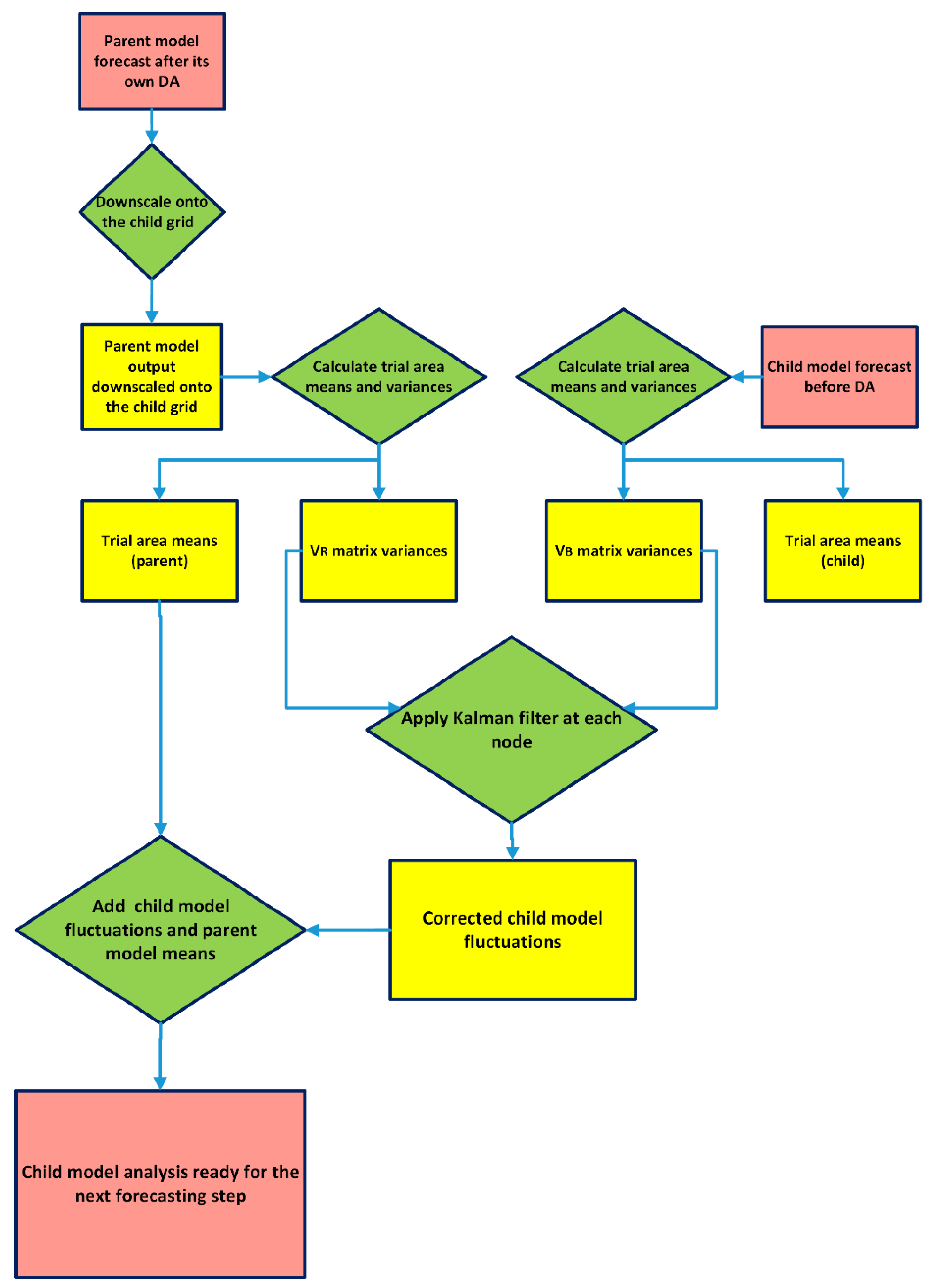
2.1. The NDA Algorithm
2.2. Data for the Synthetic Idealised Case
2.3. Case Studies
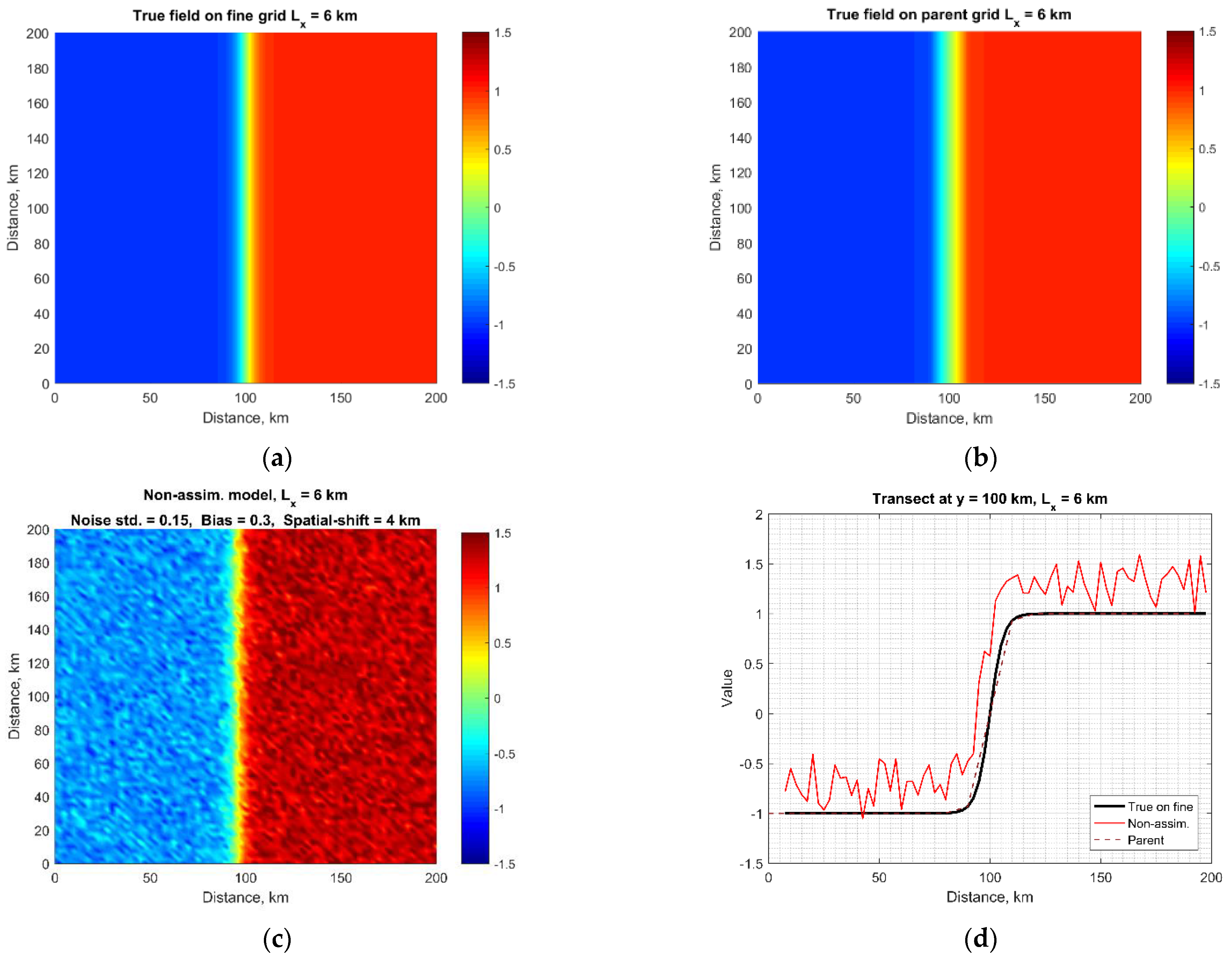
2.3.1. Ocean Front
2.3.2. Isolated Mesoscale Eddy
2.3.3. Multiple Mesoscale Eddies
3. Results
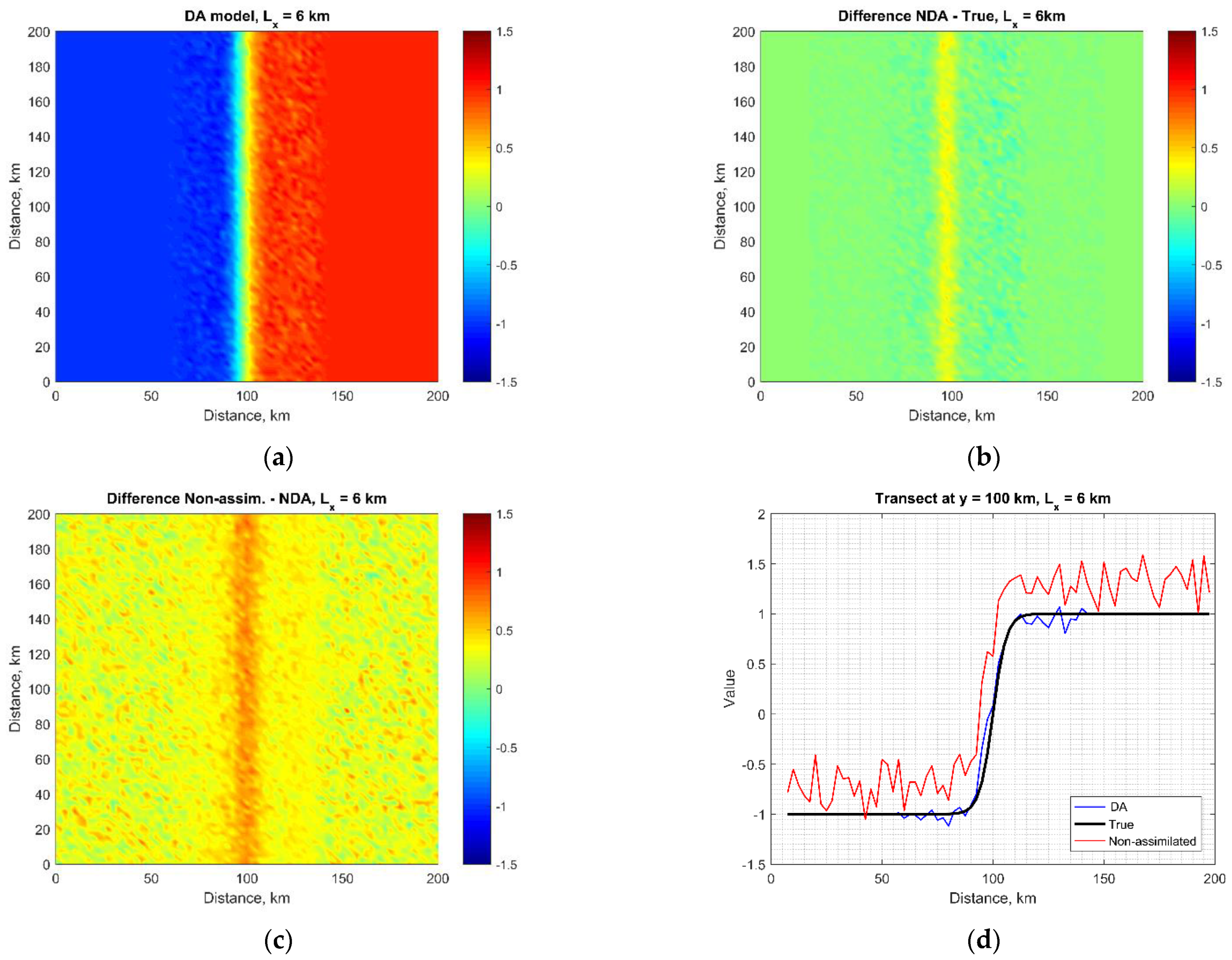
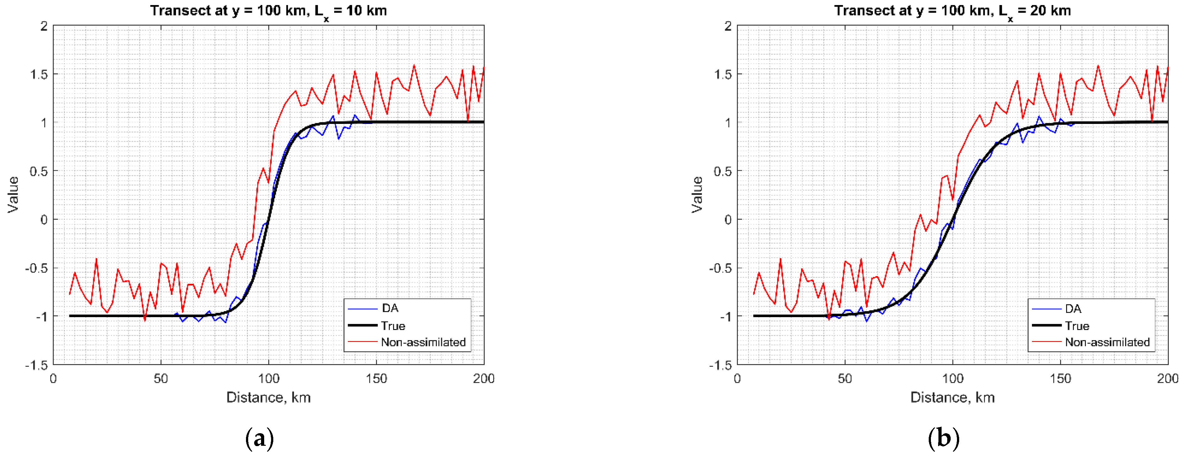
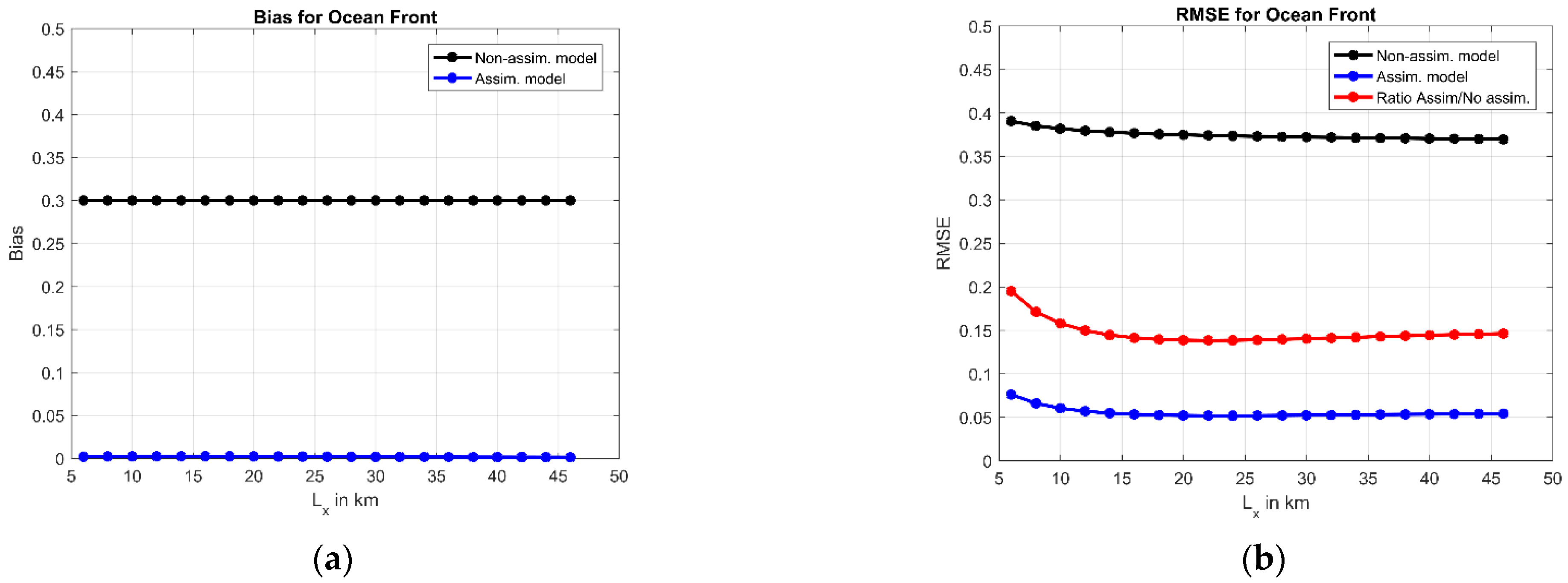
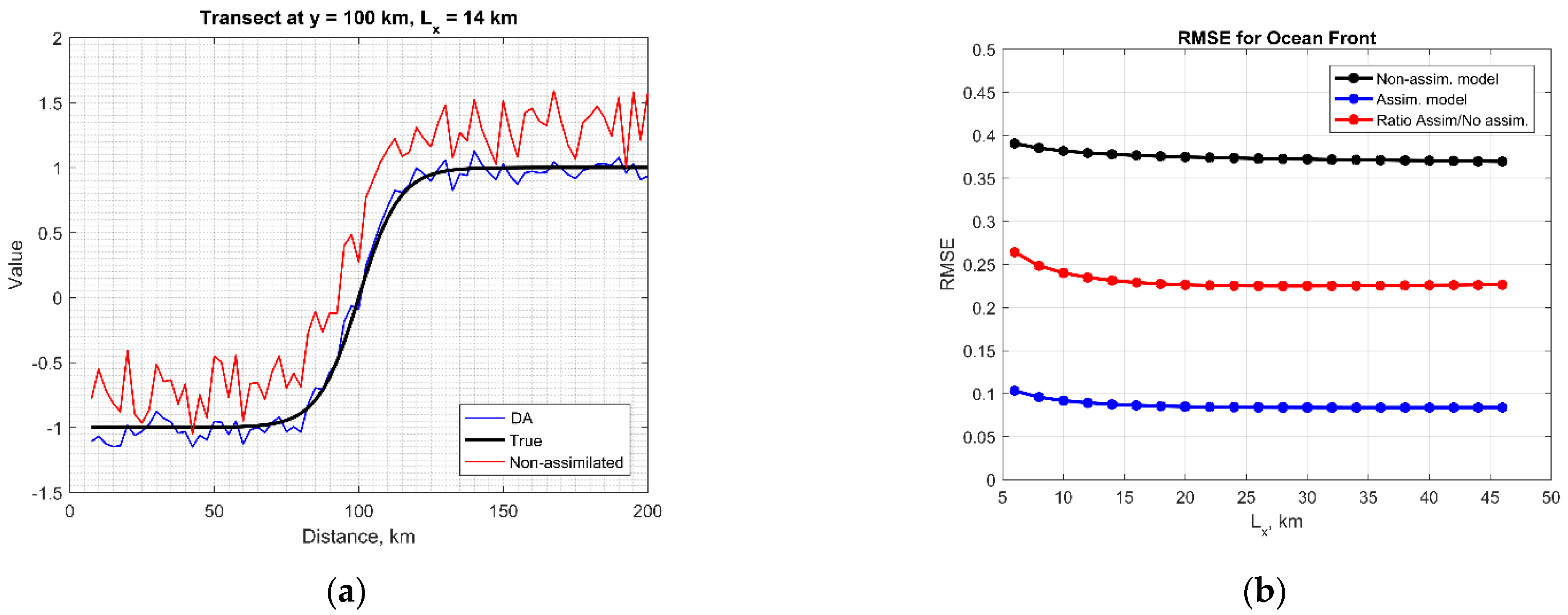
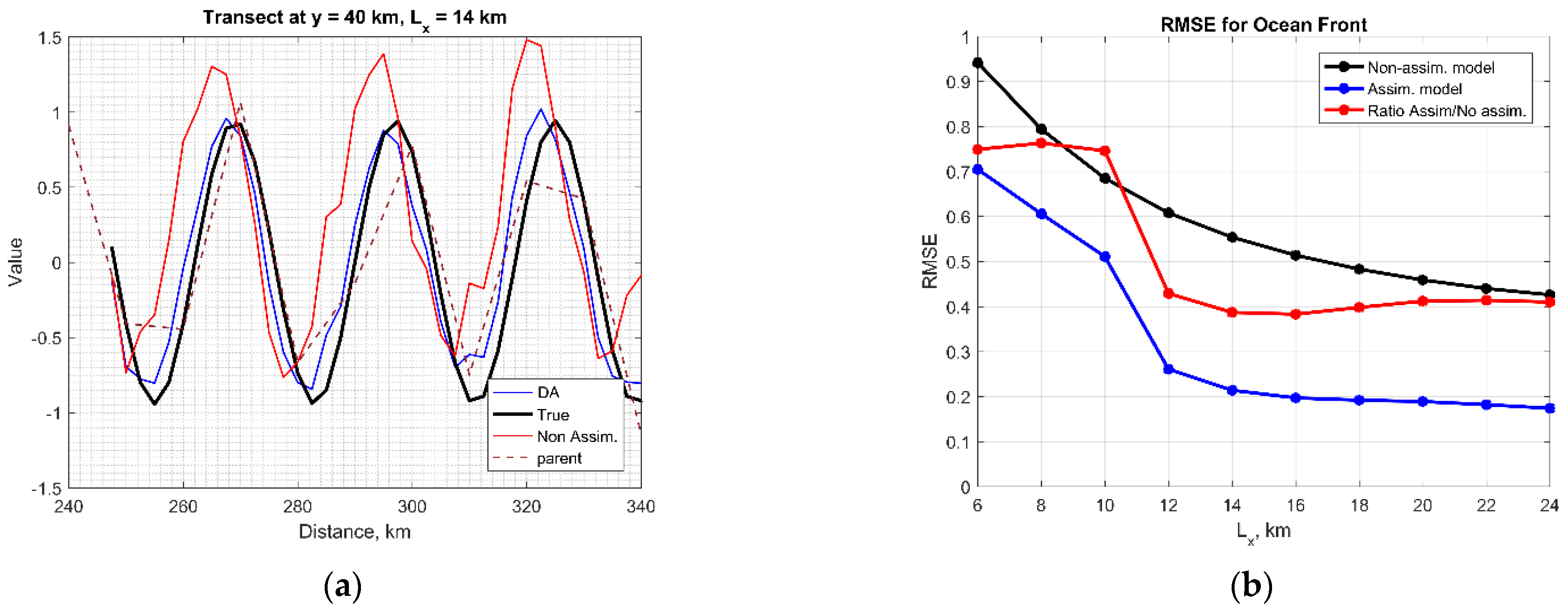
3.1. Ocean Front
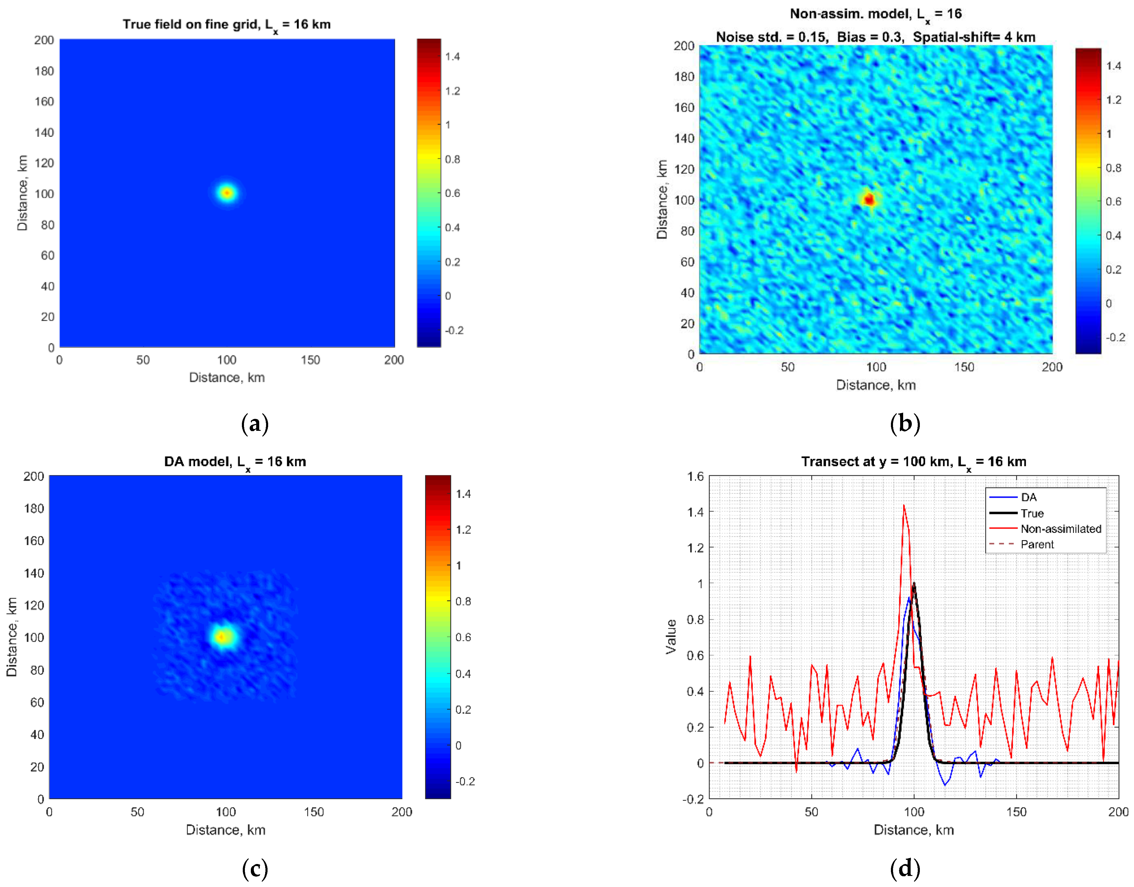
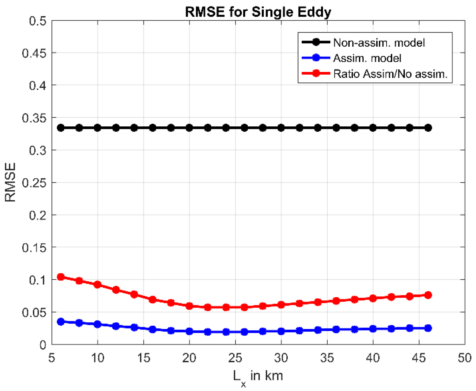
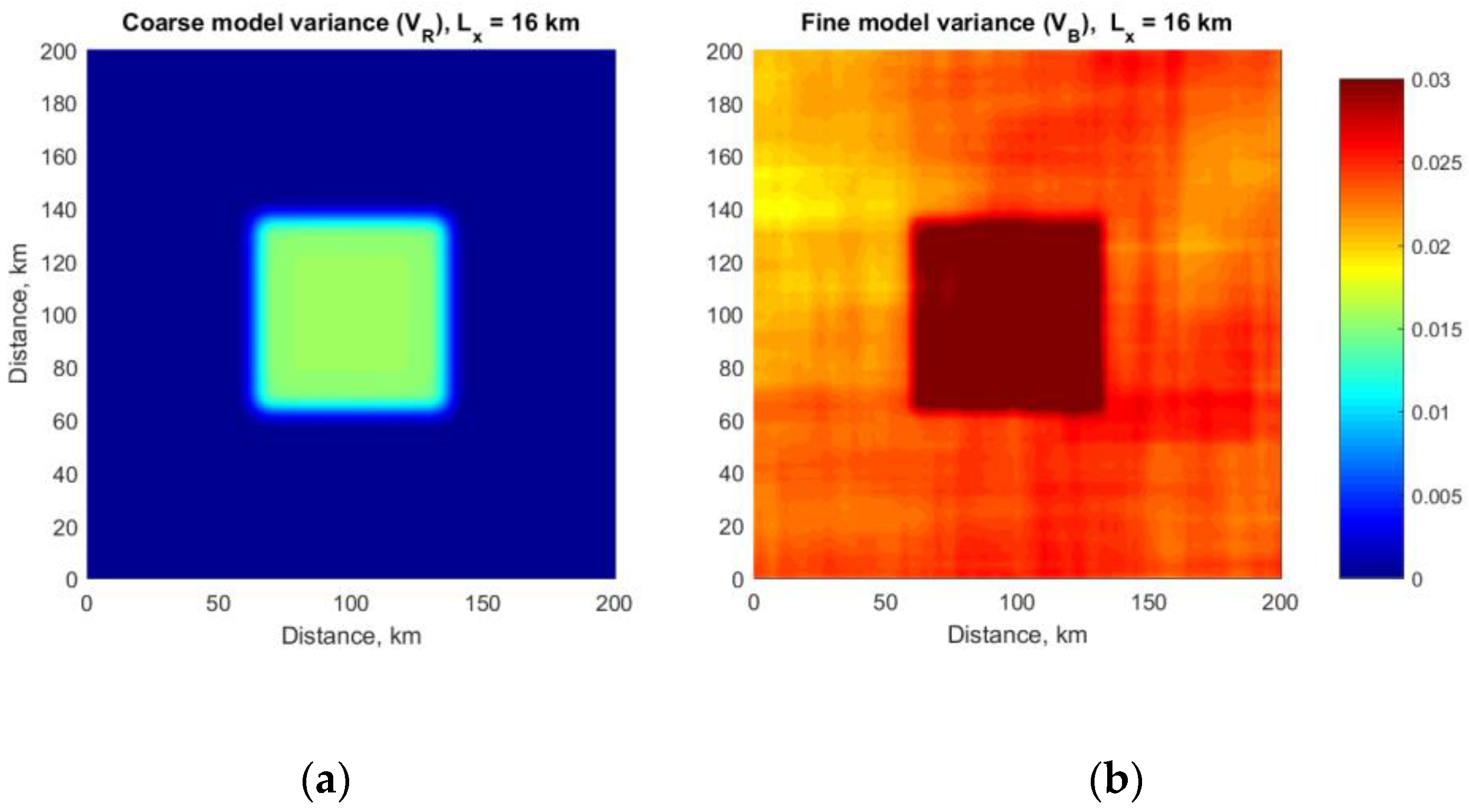
3.2. Single Eddy
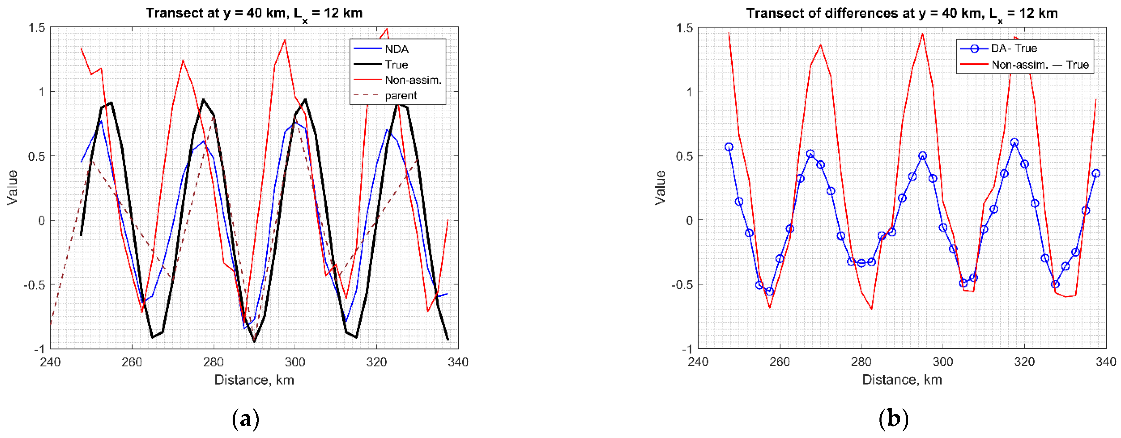
3.3. Multiple Eddies
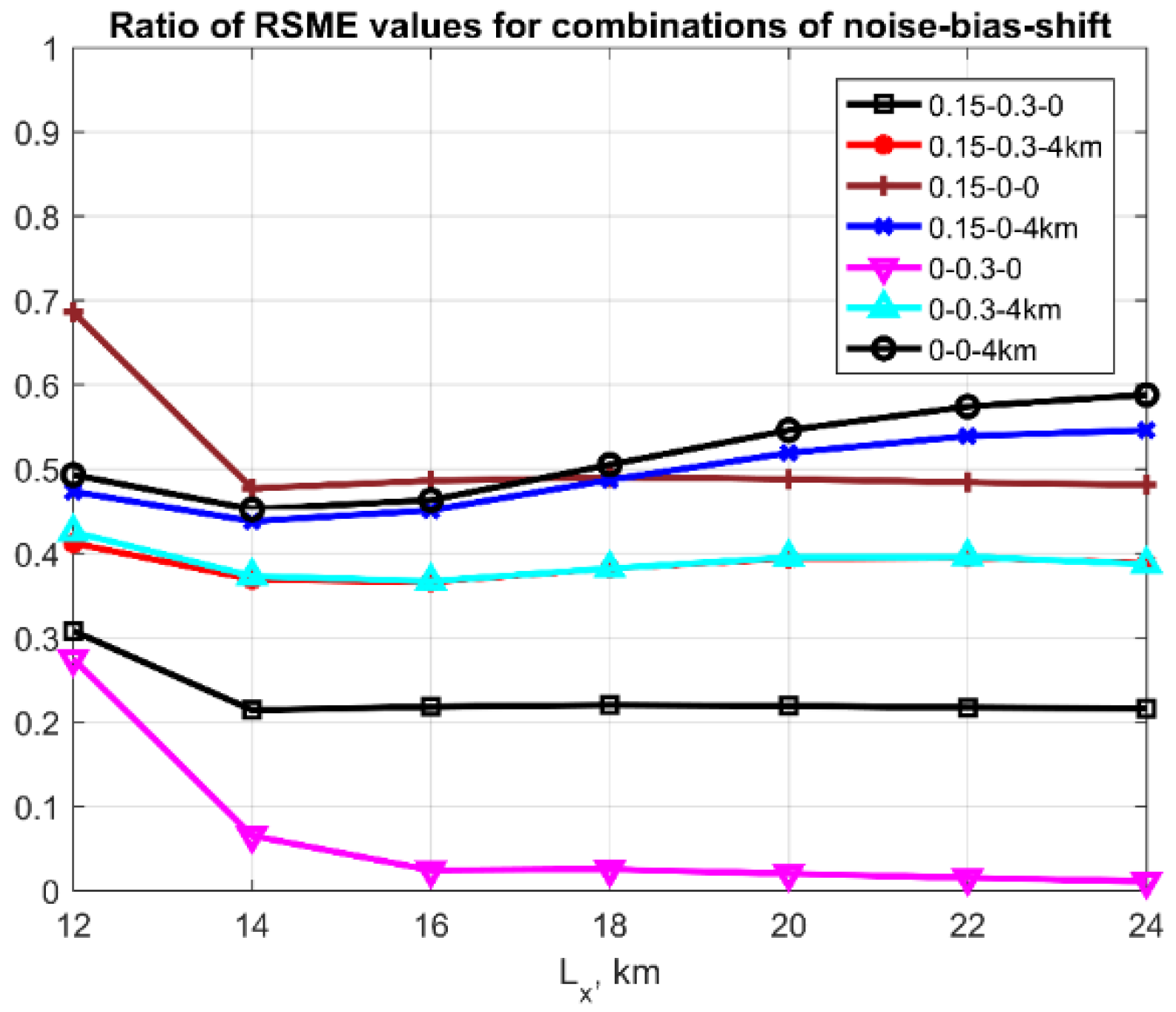
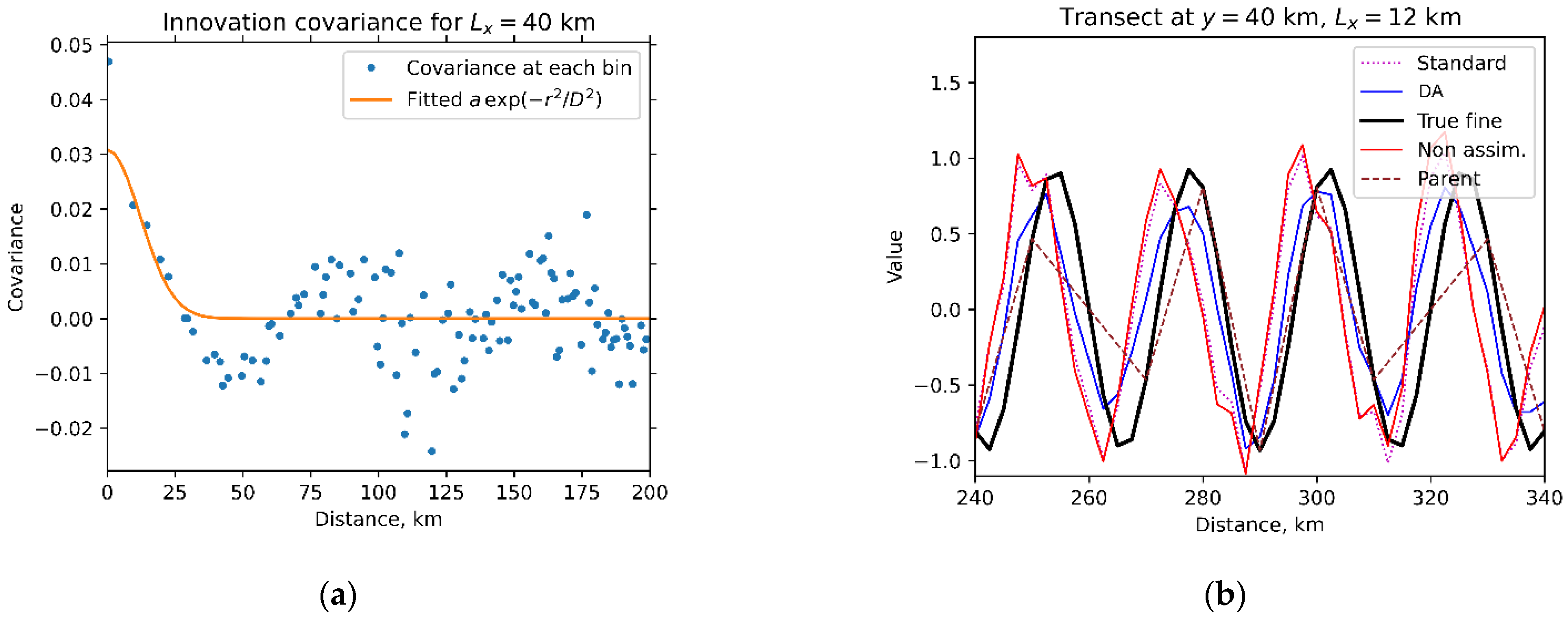
3.4. Effect of Errors in the Parent Model
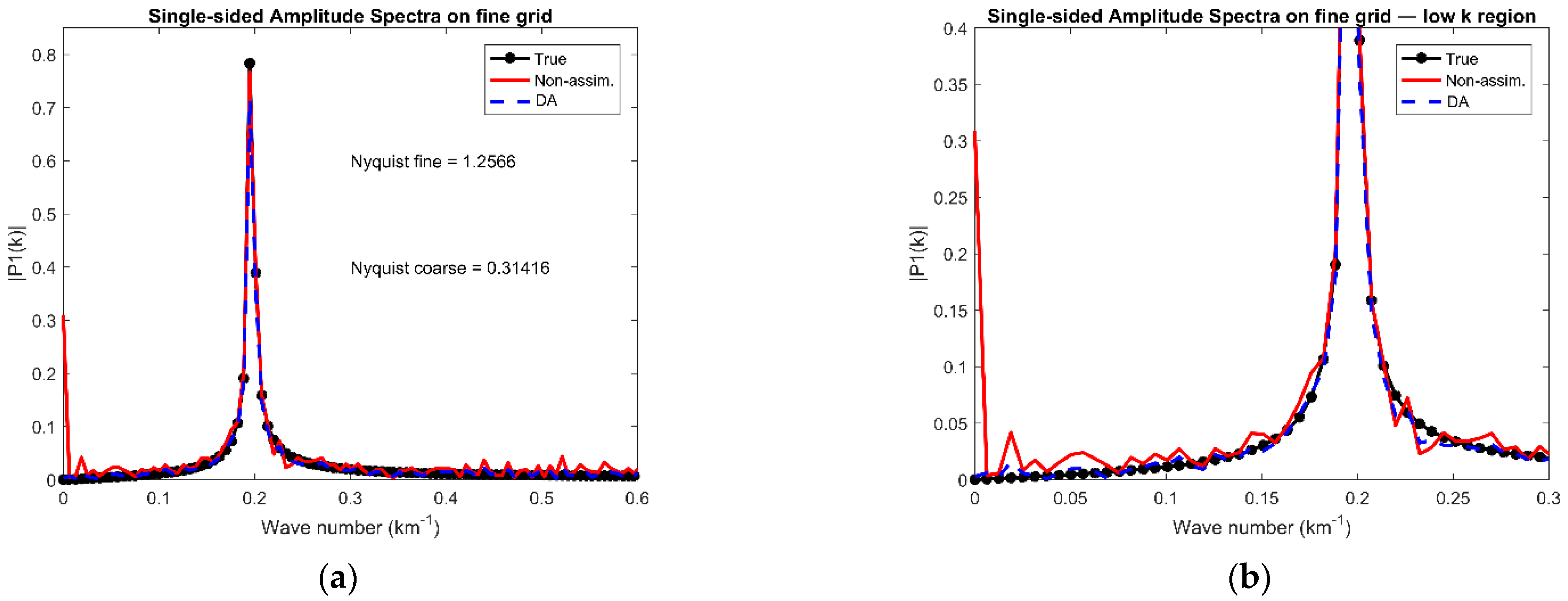
3.5. Spectral Characteristics
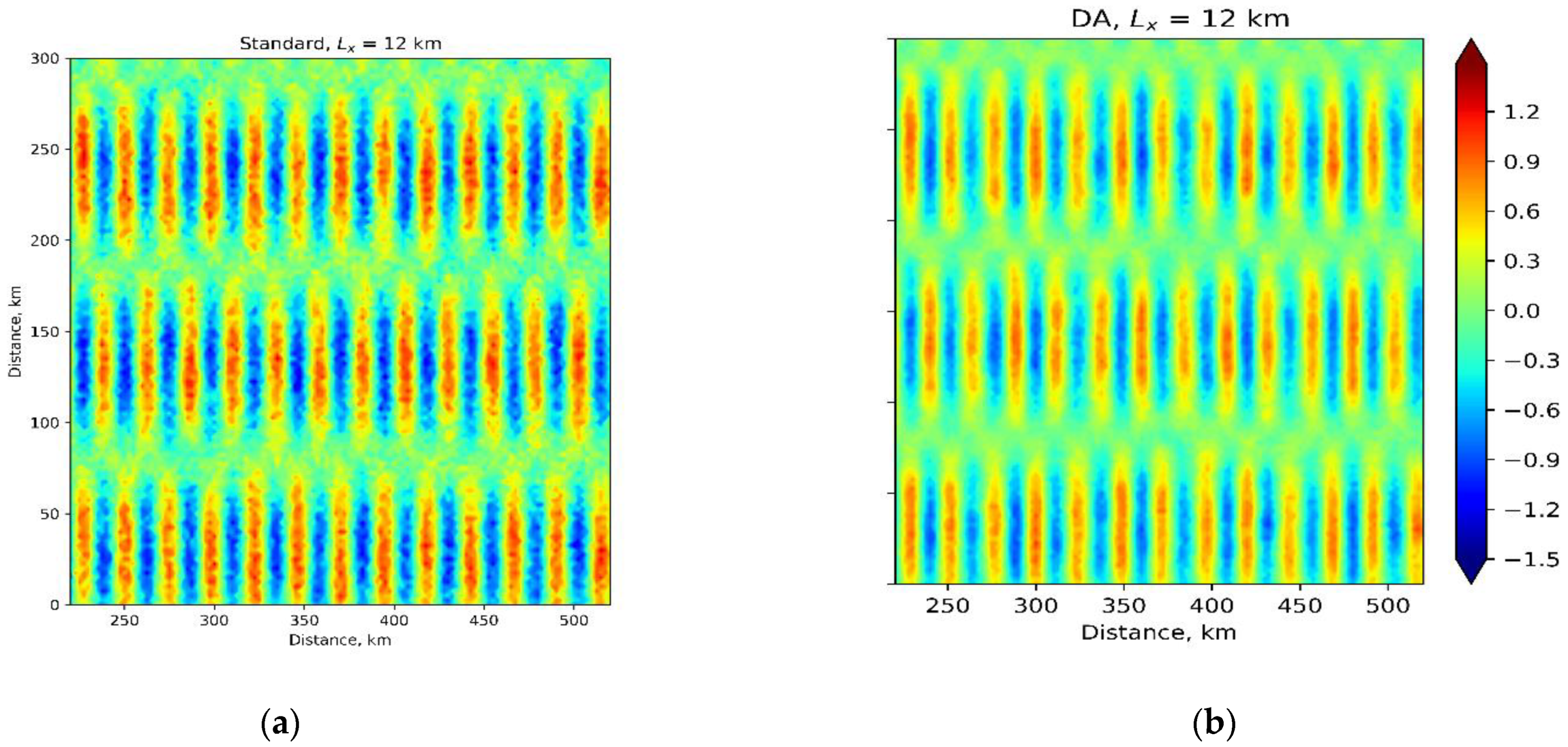
3.6. Comparison with a ‘Standard’ Method
4. Discussion
5. Conclusions
Author Contributions
Funding
Data Availability Statement
Acknowledgments
Conflicts of Interest
References
- GFDL. High-Resolution Modeling. 2020. Available online: https://www.gfdl.noaa.gov/high-resolution-modeling (accessed on 6 July 2020).
- Dufour, C.O.; Griffies, S.; de Souza, G.; Frenger, I.; Morrison, A.; Palter, J.; Sarmiento, J.L.; Galbraith, E.; Dunne, J.P.; Anderson, W.G.; et al. Role of mesoscale eddies in cross-frontal transport of heat and biogeochemical tracers in the Southern Ocean. J. Phys. Oceanogr. 2015, 45, 3057–3081. [Google Scholar] [CrossRef] [Green Version]
- Shapiro, G.I.; Stanichny, S.; Stanychna, R.R. Anatomy of shelf–deep sea exchanges by a mesoscale eddy in the North West Black Sea as derived from remotely sensed data. Remote Sens. Environ. 2010, 114, 867–875. [Google Scholar] [CrossRef]
- Meunier, T.; Barton, E.D.; Barreiro, B.; Torres, R. Upwelling filaments off Cap Blanc: Interaction of the NW African upwelling current and the Cape Verde frontal zone eddy field? J. Geophys. Res. Atmos. 2012, 117, C08031. [Google Scholar] [CrossRef] [Green Version]
- NEMO. Annual Mean of Sea Surface Salinity in 1/12° (NEMO-WRF Coupling). Available online: https://www.nemo-ocean.eu (accessed on 16 June 2021).
- ROMS. Regional Ocean Modeling System (ROMS). Available online: https://www.myroms.org (accessed on 16 June 2021).
- CMEMS. Ocean Explainers: Oceanography Educational Webpages. Available online: https://marine.copernicus.eu (accessed on 20 May 2021).
- DARC. What Is Data Assimilation? Available online: https://research.reading.ac.uk/met-darc/aboutus/what-is-data-assimilation (accessed on 5 August 2021).
- Lorenc, A.C. Analysis methods for numerical weather prediction. Q. J. R. Meteorol. Soc. 1986, 112, 1177–1194. [Google Scholar] [CrossRef]
- Bell, M.J.; Forbes, R.M.; Hines, A. Assessment of the FOAM global data assimilation system for real-time operational ocean forecasting. J. Mar. Syst. 2000, 25, 1–22. [Google Scholar] [CrossRef]
- Gandin, L.S. The problem of optimal interpolation, Scientific papers. Main Geophys. Obs. 1959, 99, 67–75. [Google Scholar]
- Moore, A.M.; Martin, M.J.; Akella, S.; Arango, H.G.; Balmaseda, M.A.; Bertino, L.; Ciavatta, S.; Cornuelle, B.; Cummings, J.; Frolov, S.; et al. Synthesis of Ocean Observations Using Data Assimilation for Operational, Real-Time and Reanalysis Systems: A More Complete Picture of the State of the Ocean. Front. Mar. Sci. 2019, 6, 90. [Google Scholar] [CrossRef] [Green Version]
- Dobricic, S.; Pinardi, N. An oceanographic three-dimensional variational data assimilation scheme. Ocean. Model 2008, 22, 89–105. [Google Scholar] [CrossRef]
- Ghil, M.; Malanotte-Rizzoli, P. Data Assimilation in Meteorology and Oceanography. Adv. Geophys. 1991, 33, 141–266. [Google Scholar] [CrossRef]
- NEMOVAR. The NEMOVAR Ocean Data Assimilation System as Implemented in the ECMWF Ocean Analysis for System 4. Available online: https://www.ecmwf.int/en/elibrary/11174-nemovar-ocean-data-assimilation-system-implemented-ecmwf-ocean-analysis-system-4 (accessed on 1 October 2021).
- DART, Data Assimilation Research Testbed. Available online: https://dart.ucar.edu (accessed on 1 October 2021).
- PDAF, Parallel Data Assimilation Network. Available online: https://pdaf.awi.de/trac/wiki (accessed on 1 October 2021).
- Bannister, R.N. A review of forecast error covariance statistics in atmospheric variational data assimilation. II: Modelling the forecast error covariance statistics. Q. J. R. Meteorol. Soc. 2008, 134, 1971–1996. [Google Scholar] [CrossRef]
- Waters, J.; Lea, D.J.; Martin, M.J.; Mirouze, I.; Weaver, A.; While, J. Implementing a variational data assimilation system in an operational 1/4 degree global ocean model. Q. J. R. Meteorol. Soc. 2015, 141, 333–349. [Google Scholar] [CrossRef]
- Haben, S.; Lawless, A.; Nichols, N. Conditioning and preconditioning of the variational data assimilation problem. Comput. Fluids 2011, 46, 252–256. [Google Scholar] [CrossRef]
- Kubryakov, A.I.; Korotaev, G.K.; Dorofeev, V.L.; Ratner, Y.B.; Palazov, A.; Valchev, N.; Malciu, V.; Mateescu, R.; Oguz, T. Black Sea coastal forecasting system. Ocean Sci. 2012, 8, 183–196. [Google Scholar] [CrossRef] [Green Version]
- Carrassi, A.; Bocquet, M.; Bertino, L.; Evensen, G. Data assimilation in the geosciences: An overview of methods, issues, and perspectives. WIREs Clim. Chang. 2018, 9, e535. [Google Scholar] [CrossRef] [Green Version]
- Bouttier, F.; Courtier, P. Data Assimilation Concepts and Methods. 1999. Available online: https://www.ecmwf.int/en/elibrary/16928-data-assimilation-concepts-and-methods (accessed on 5 August 2021).
- Hollingsworth, A.; Lönnberg, P. The statistical structure of short-range forecast errors as determined from radiosonde data, Part 1: The wind field. Tellus A 1986, 38, 111–136. [Google Scholar] [CrossRef] [Green Version]
- Kalnay, E. Atmospheric Modeling, Data Assimilation and Predictability; Cambridge University Press (CUP): Cambridge, UK, 2003; 369p. [Google Scholar]
- Shapiro, G.I.; Gonzalez-Ondina, J.M.; Belokopytov, V.N. High-resolution stochastic downscaling method for ocean forecasting models and its application to the Red Sea dynamics. Ocean Sci. 2021, 17, 891–907. [Google Scholar] [CrossRef]
- Parrish, D.F.; Derber, J.C. The National Meteorological Center’s spectral statistical interpolation analysis system. Mon. Weather Rev. 1992, 120, 1747–1763. [Google Scholar] [CrossRef]
- Polavarapu, S.; Ren, S.; Rochon, Y.; Sankey, D.; Ek, N.; Koshyk, J.; Tarasick, D. Data assimilation with the Canadian middle atmosphere model. Atmosphere-Ocean 2005, 43, 77–100. [Google Scholar] [CrossRef]
- Zingerlea, C.; Nurmib, P. Monitoring and verifying cloud forecasts originating from operational numerical models. Meteorol. Appl. 2008, 15, 325–330. [Google Scholar] [CrossRef]
- Bruciaferri, D.; Shapiro, G.; Wobus, F. A multi-envelope vertical coordinate system for numerical ocean modelling. Ocean Dyn. 2018, 68, 1239–1258. [Google Scholar] [CrossRef] [Green Version]
- Mellor, G.L.; Blumberg, A.F. Modeling Vertical and Horizontal Diffusivities with the Sigma Coordinate System. Mon. Weather Rev. 1985, 113, 1379–1383. [Google Scholar] [CrossRef]
- Adhikary, B.; Kulkarni, S.; Dallura, A.; Tang, Y.; Chai, T.; Leung, L.; Qian, Y.; Chung, C.; Ramanathan, V.; Carmichael, G. A regional scale chemical transport modeling of Asian aerosols with data assimilation of AOD observations using optimal interpolation technique. Atmos. Environ. 2008, 42, 8600–8615. [Google Scholar] [CrossRef]
- Fedorov, K.N. The Physical Nature and Structure of Oceanic Fronts; Springer: Berlin/Heidelberg, Germany, 1986; 333p, ISBN 978-0-387-96445-4. [Google Scholar]
- Robinson, A.R. (Ed.) . Eddies in Marine Science; Springer: Berlin/Heidelberg, Germany, 1983; 612p, ISBN 978-3-642-69003-7. [Google Scholar]
- Stewart, L.M.; Dance, S.L.; Nichols, N.K.; Eyre, J.R.; Cameron, J. Estimating interchannel observation-error correlations for IASI radiance data in the Met Office system. Q. J. R. Meteorol. Soc. 2014, 140, 1236–1244. [Google Scholar] [CrossRef] [Green Version]
- Stull, R.B. An introduction to boundary layer meteorology. Kluwer 2003, 670. [Google Scholar] [CrossRef]
- Katavouta, A.; Thompson, K.R. Downscaling ocean conditions with application to the Gulf of Maine, Scotian Shelf and adjacent deep ocean. Ocean Model. 2016, 104, 54–72. [Google Scholar] [CrossRef] [Green Version]
- Global Ocean Physics Reanalysis (GLOBAL_MULTIYEAR_PHY_001_030). Available online: https://resources.marine.copernicus.eu/product-detail/GLOBAL_MULTIYEAR_PHY_001_030/INFORMATION (accessed on 7 March 2022).
- Stommel, H. The westward intensification of wind-driven ocean currents. Trans. Am. Geophys. Union 1948, 29, 202–206. [Google Scholar] [CrossRef]
- Shapiro, G.I.; Ondina, J.M.; Poovadiyil, M.S.; Tu, J.; Asif, M. The Operational Ocean Modelling System of the Lakshadweep Sea; University of Plymouth: Plymouth, UK, 2022; (Manuscript in Preparation). [Google Scholar]


| Forecast (before DA) | ‘Standard’ DA | NDA | |
|---|---|---|---|
| Bias | 0.300 | −0.0066 | 0.000 |
| RMSE | 0.608 | 0.5268 | 0.250 |
Publisher’s Note: MDPI stays neutral with regard to jurisdictional claims in published maps and institutional affiliations. |
© 2022 by the authors. Licensee MDPI, Basel, Switzerland. This article is an open access article distributed under the terms and conditions of the Creative Commons Attribution (CC BY) license (https://creativecommons.org/licenses/by/4.0/).
Share and Cite
Shapiro, G.I.; Gonzalez-Ondina, J.M. An Efficient Method for Nested High-Resolution Ocean Modelling Incorporating a Data Assimilation Technique. J. Mar. Sci. Eng. 2022, 10, 432. https://doi.org/10.3390/jmse10030432
Shapiro GI, Gonzalez-Ondina JM. An Efficient Method for Nested High-Resolution Ocean Modelling Incorporating a Data Assimilation Technique. Journal of Marine Science and Engineering. 2022; 10(3):432. https://doi.org/10.3390/jmse10030432
Chicago/Turabian StyleShapiro, Georgy I., and Jose M. Gonzalez-Ondina. 2022. "An Efficient Method for Nested High-Resolution Ocean Modelling Incorporating a Data Assimilation Technique" Journal of Marine Science and Engineering 10, no. 3: 432. https://doi.org/10.3390/jmse10030432