Article

Application of Radar Image Fusion Method to Near-Field Sea Ice Warning for Autonomous Ships in the Polar Region

Merchant Marine College, Shanghai Maritime University, Shanghai 201306, China
*
Authors to whom correspondence should be addressed.
J. Mar. Sci. Eng. 2022, 10(3), 421; https://doi.org/10.3390/jmse10030421
Submission received: 8 January 2022 / Revised: 9 March 2022 / Accepted: 10 March 2022 / Published: 14 March 2022
(This article belongs to the Special Issue Control Theory and Applications in Marine Autonomous Vehicles)

Abstract

:
Mastering the real-time dynamics of near-field sea ice is the primary condition to guaranteeing the navigation safety of autonomous ships in the polar region. In this study, a radar image fusion process combining marine radar and ice radar is proposed, which can effectively solve the problems of redundant information and spatial registration during image fusion. Then, using the fused radar images, this study proposes a set of near-field sea ice risk assessment and warning processes applicable to both low- and high-sea-ice-concentration situations. The sea ice risk indexes in these two situations are constructed by using four variables: sea ice area, sea ice grayscale, distance between sea ice and the own-ship, and relative bearing of sea ice and the own-ship. Finally, visualization processing is carried out according to the size of the risk index values of each piece of sea ice to achieve a better near-field sea ice risk assessment and warning effect. According to the example demonstration results, through the radar image fusion process and the set of near-field sea ice risk assessment and warning processes proposed in this study, the sea ice risk distribution in the near-field area of the ship can be well obtained, which provides effective support for the assisted decision-making of autonomous navigation in the polar region.

1. Introduction

In recent years, with the continuous warming of the global climate, much research data have shown that the extent of sea ice in the Arctic and Antarctica has decreased dramatically [1,2,3], and many studies have even predicted that the Arctic Ocean will be ice-free in summer within 15 years [4]. As the sea ice in the polar region gradually decreases, the number of voyages into the polar region also gradually increases. In the Arctic region, the Arctic shipping route has the economic benefit of greatly shortening the route distance between the three major economic circles of Northeast Asia, Europe, and North America. In the Antarctic region, the number of people engaged in scientific research and tourism activities has also increased year by year. Although global warming has increased the possibility of polar navigation, sea ice remains a key factor affecting navigation safety in the polar region. In order to ensure navigation safety, it is of great significance to conduct near-field sea ice perception and warning research, which is also one of the key technologies for the development of autonomous ships in the polar region.
To realize the autonomous and unmanned ship, the technology of perception, decision-making, and control must be developed, and the quality of perception information is the source and key to determine the effect of decision-making and control. The sensing equipment of autonomous ships can be divided into two types: shipboard sensors and satellite-based sensors [5]. Shipboard sensors include the very high frequency (VHF) radio-based automatic identification system (AIS), electronic chart display and information system (ECDIS) [6], marine radar, attitude indicator, and depth sounder. Satellite-based sensors include the global navigation satellite system (GNSS), satellite-based AIS [7], the meteorological and oceanographic (METOC) data receiver, synthetic aperture radar (SAR), and the long-range identification and tracking (LRIT) system. In general, different sensors have different detection objects, data types, and applicability, and not all of them are suitable for the ice detection requirements of polar autonomous ships.
This study summarizes and compares the related studies on sea ice risk warning, as shown in Table 1. According to the sensing range of sea ice by the sensing equipment, it can be divided into three categories: large-scale sea ice data, medium-scale sea ice data, and small-scale sea ice data. Among them, the large-scale sea ice data are acquired mainly through a satellite remote sensing method such as NOAA (the National Oceanic and Atmospheric Administration satellite) [8], RADARSAT (Canada’s satellite) [9], and MODIS (the moderate resolution imaging spectroradiometer on board NASA’s satellite) [10], which is not affected by polar night and weather, is widely used to retrieve the information of sea ice concentration [9,11,12,13,14,15] and thickness/grayscale [8,16,17,18,19], and monitors the spatial-temporal changes in sea ice conditions. However, its temporal resolution is usually one day, which is more suitable for grasping the large-scale sea ice range, but poor in grasping near-field and real-time sea ice conditions. The small-scale sea ice data are acquired mainly through the shipboard or airborne camera [20,21,22], which is the observation method closest to human eyes and can accurately obtain the close-range sea ice image in the near-field area of the ship. However, due to its short viewing distance and inability to obtain extensive and complete sea ice information, it is more suitable for verifying ice conditions. The medium-scale sea ice data are acquired mainly through the airborne electromagnetic induction device (i.e., a so-called EM-bird) [23], marine radar, ice radar, etc. Compared with the other two categories of data, it can better grasp the near-field sea ice conditions in real time.
In fact, radar is sensing equipment suitable for ice detection in the near-field waters [24]. It is clearly stated in the International Code for Ships Operating in Polar Waters (Polar Code) that ships sailing in polar waters should be actively equipped with radars with ice detection capabilities [25]. Compared with the research that only uses a single-sensor marine radar to obtain ice information [26], this study uses the fused image of the marine radar and the ice radar, which can provide more comprehensive sea ice information for the near-field sea ice perception.
In addition, what variables should be considered when conducting near-field sea ice risk warning studies? As can be seen from Table 1, although most studies have taken into account the impact of sea ice physical characteristics such as sea ice concentration and sea ice area on sea ice risk when conducting sea ice risk assessment [8,9,10,11,12,13,14,15,16,18,19,20,21,22,23,26,27], they have not considered the relationship between the own-ship and sea ice from the point of view of navigation safety and the perspective of navigators. As for the differences in different sea ice concentration situations, the sea ice risk assessment and warning methods should also be considered and dealt with separately.
Based on this, this study uses the fused radar image, takes into account the risk variables such as sea ice concentration, sea ice area, sea ice grayscale, and the newly added risk variables such as the distance between sea ice and the own-ship and the relative bearing of sea ice and the own-ship, and proposes a set of near-field sea ice risk assessment and warning processes that meet the needs of autonomous ships in the polar region and are suitable for two situations. Ships can choose to adopt nonpartition or partition sea ice risk assessment methods according to the actual sea ice concentration in the near-field waters to ensure effective warning of sea ice risks and guarantee navigation safety.
Table 1. Comparison of studies related to sea ice risk warning.
Related StudiesSensing RangeSensing EquipmentMulti-Source DataSIC 1SIA 2SIG 3Dist 4Relative BearingVisual Warning
Haverkamp et al. (1995) [19]LargeSatellite (SAR)XXOOXXX
Spreen et al. (2008) [11]LargeSatellite (AMSR-E sensor)XOOXXXO
Gu et al. (2013) [8]LargeNOAA satelliteXXOOXXO
Beitsch et al. (2014) [12]LargeSatellite (AMSR-2 sensor)XOXXXXO
Posey et al. (2015) [13]LargeSatellite (AMSR-2 and SSMIS sensors)OOXXXXO
Hebert et al. (2015) [14]LargeSatellite (AMSR-2 sensor)OOXXXXO
Wang et al. (2016) [9]LargeSatellite (SAR- RADARSAT-2)XOXXXXO
Zeng et al. (2016) [10]LargeTerra satellite (MODIS sensors)XOXOXXO
Chi et al. (2017) [15]LargeSatellite (passive microwave sensors)XOXXXXO
Yan et al. (2019) [18]LargeCOMS satellite (GOCI)XXOOXXO
Dumitru et al. (2019) [27]LargeSentinel-1 satellite (SAR)XXOOXXO
Xiao et al. (2021) [16]LargeCryoSat-2 satelliteXXXOXXO
Weissling et al. (2009) [20]SmallCamera observationXXOOXXO
Zhang and Skjetne. (2015) [21]SmallCamera observationXXOOXXO
Parmiggiani et al. (2019) [22]SmallCamera observationXXOXXXO
Renner et al. (2013) [23]MediumEM-bird sensor and camera observation OXOOXXO
Hsieh et al. (2021) [26]MediumMarine radarXXOXOXO
This studyMediumMarine radar and ice radarOOOOOOO
1 Sea ice concentration; 2 Sea ice area; 3 Sea ice grayscale or thickness; 4 Distance between sea ice and the own-ship. Note: O—considered, X—not considered.

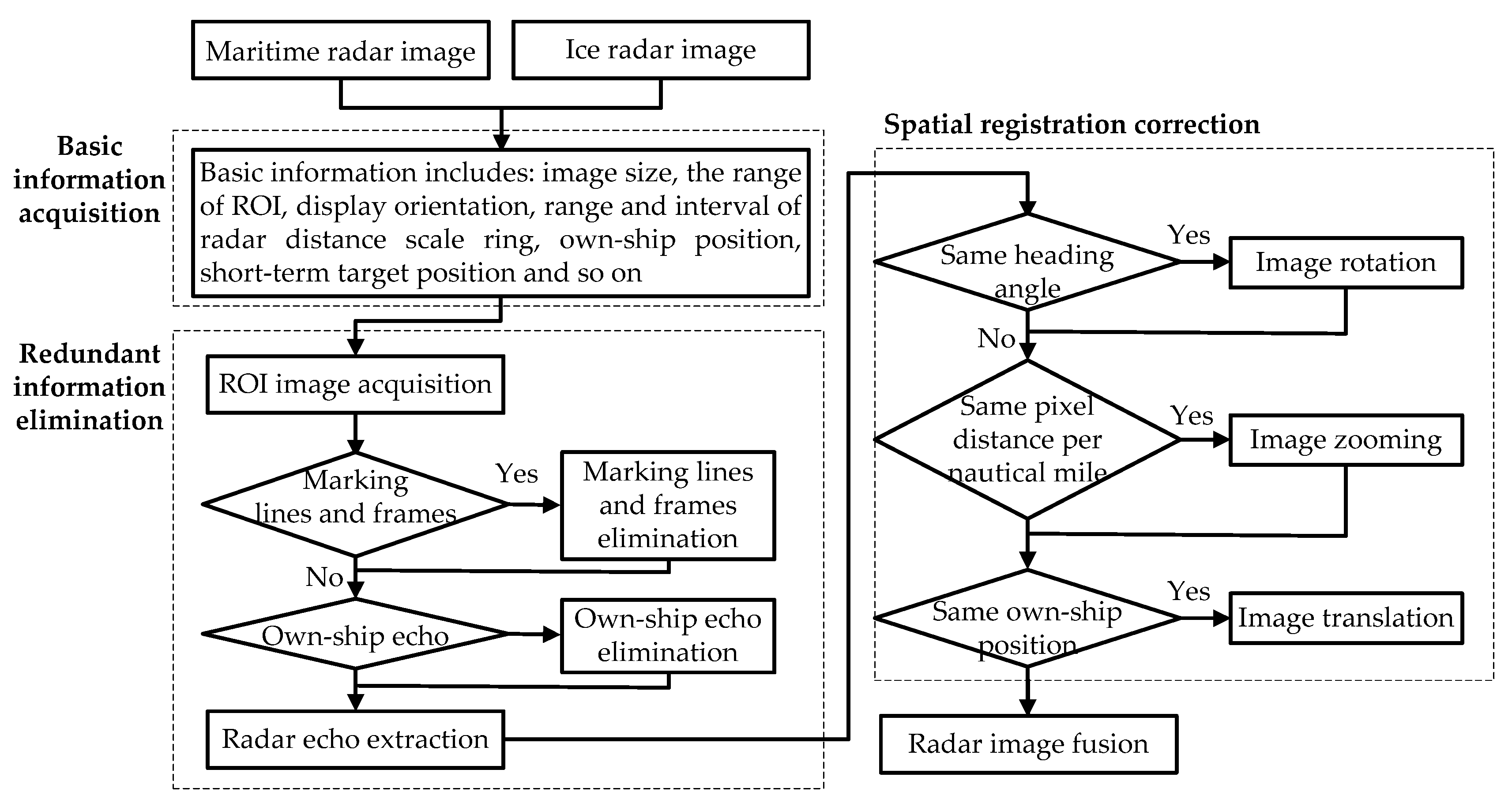
2. Radar Image Fusion Process

Radar is an effective equipment for autonomous ships in the polar region to detect the near-field sea ice targets. Among them, marine radar is a necessary navigation equipment for ships. Its detection range is farther, but the detection effect of sea ice is poor, and only part of the edge of sea ice can be delineated. Ice radar can reflect the overall ice texture better, but the detection range is closer and the noise interference is greater. Compared with a single sensor, the fusion of image information of these two radars will help to perceive the near-field sea ice scene more comprehensively. However, even if two radar images at the same time point are selected for radar image fusion, the problems of redundant information and spatial registration must be solved. The problem of redundant information is how to eliminate the interference of various redundant information and correctly extract the target echo information on the radar echo display area. The redundant information includes: (1) various menus, options, words, and numbers on the radar image; (2) the marking lines and frames on the radar echo display area; (3) the echo at the center of the radar distance scale ring may be the hull of the own-ship rather than sea ice. The spatial registration problems include: (1) as the radar display orientation may be head-up or north-up, the heading angle of the two radar images may be inconsistent; (2) as the selected range or interval of the radar distance scale ring may be different, the pixel distance corresponding to the same 1 nautical mile may be inconsistent; (3) as the radar display mode may be non-off-center or off-center, the pixel position of the center of the radar distance scale ring may be inconsistent.
In order to solve the above problems, this study proposed a radar image fusion process for near-field sea ice perception of polar autonomous ships. The process includes five steps, including radar image capture, basic information acquisition, redundant information elimination, spatial registration correction, and radar image fusion, as shown in Figure 1. These steps are explained as follows.

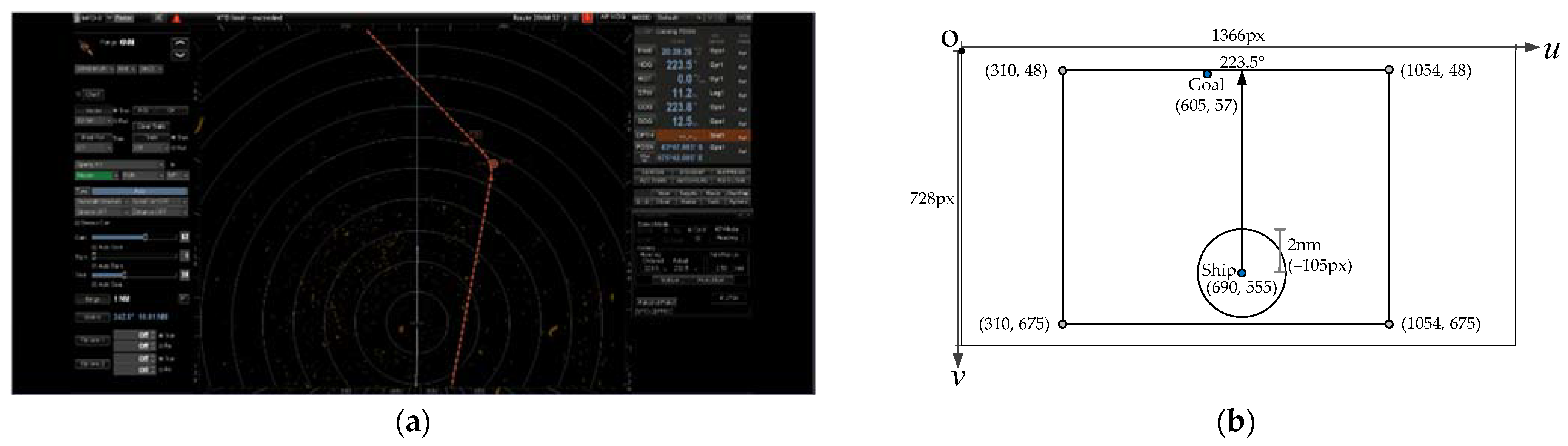
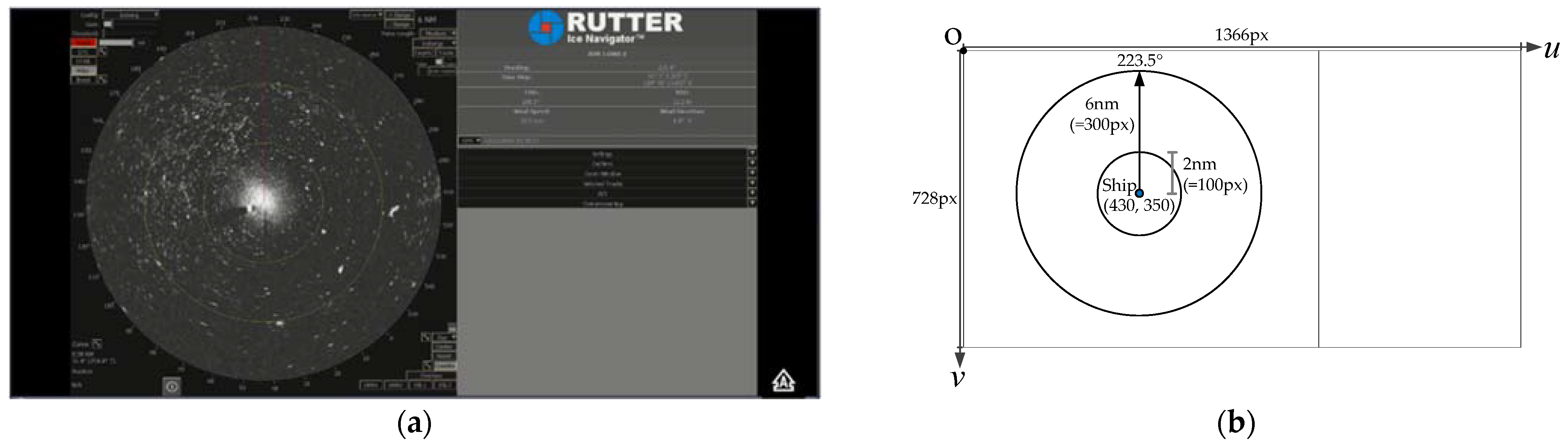
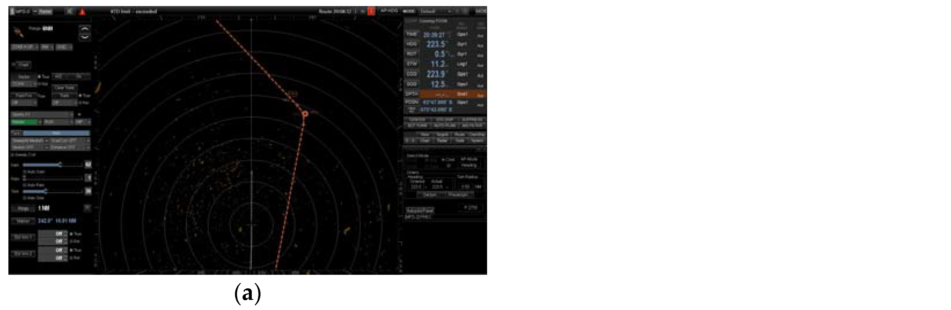
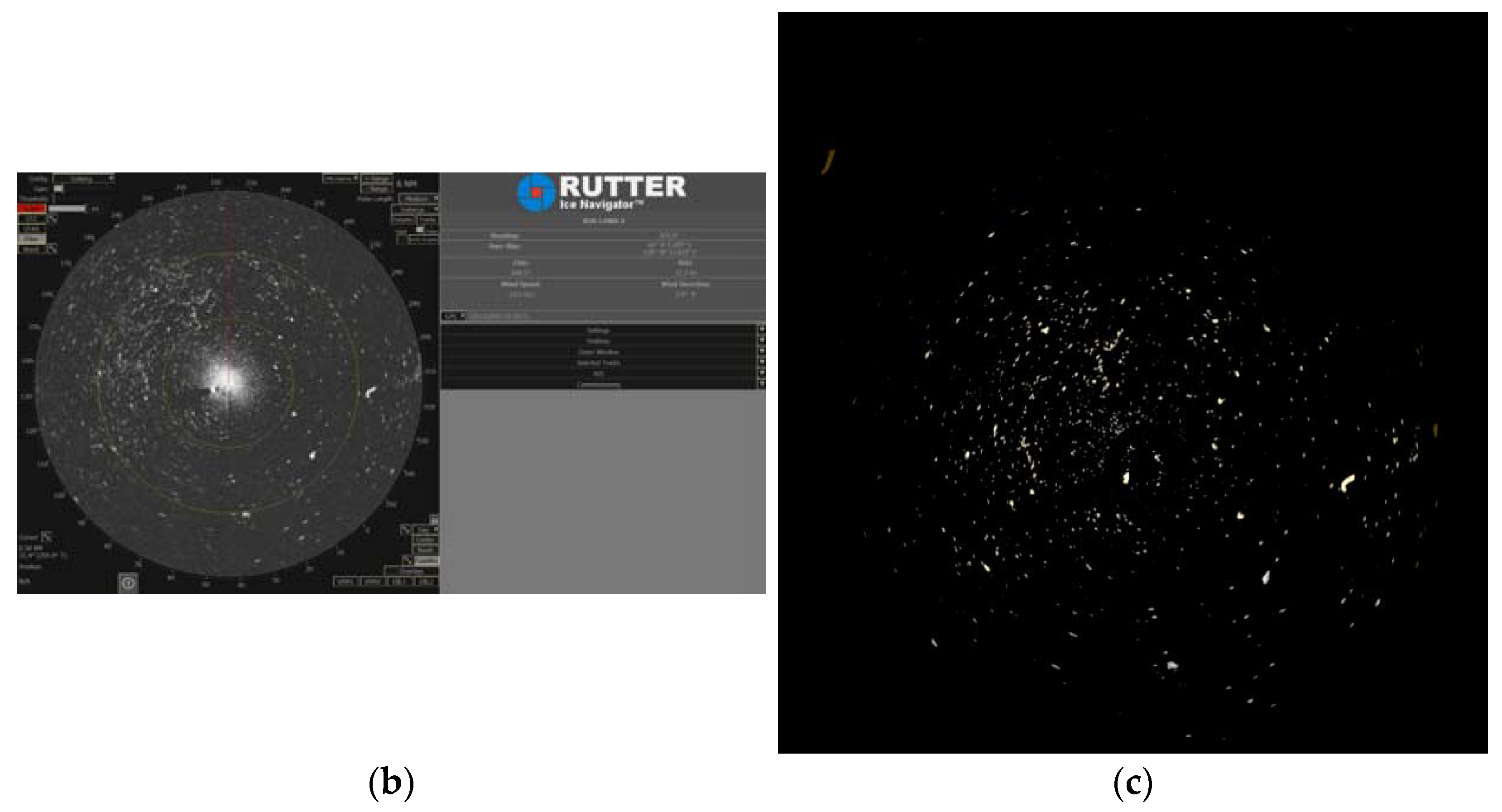
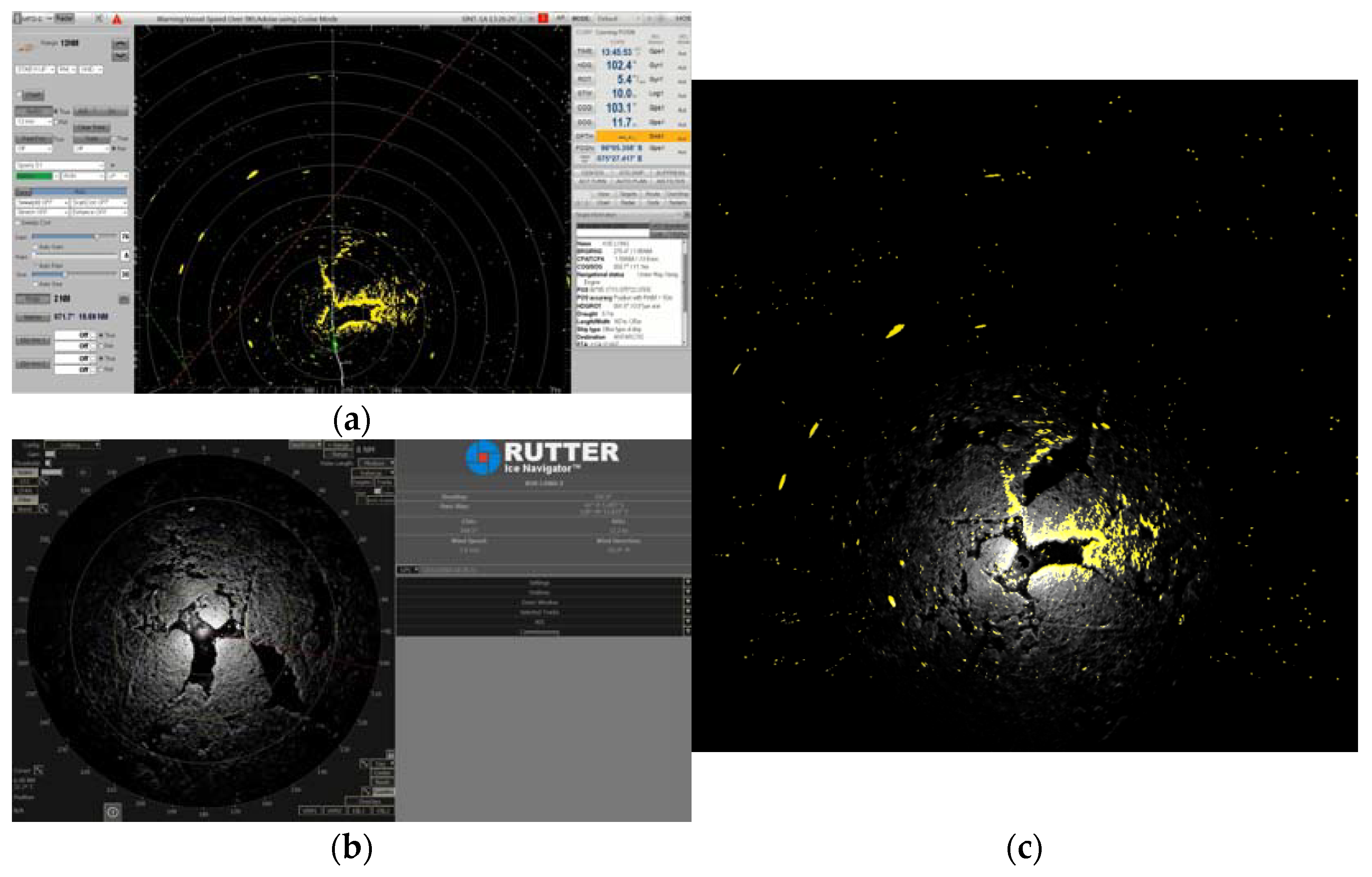
2.1. Radar Image Capture and Basic Information Acquisition

The images of marine radar and ice radar at the same time point (note that there may be a time difference between the two radars or two sensors) were captured, respectively, as shown in Figure 2a and Figure 3a; both radar images were saved in three-dimensional matrix form. Through image measurement software, the basic information such as image size, the range of region of interest (ROI), display orientation, range and interval of the radar distance scale ring, the position of the own-ship, and the short-term target position were obtained.
The basic information obtained from the marine radar image is shown in Figure 2b: the image size is 1366 × 728 pixels (px); the ROI is a rectangular region composed of four coordinate points (310, 48), (310, 675), (1054, 48), and (1054, 675); the radar display orientation is head-up and the heading angle is 223.5°; the radar display mode is off-center (that is, the center of the ring is located in the center of the screen); the range of the radar distance scale ring is set to 6 nautical miles (nm) and the ring diameter with a radius of 2 nm corresponds to 105 px; the position of the own-ship is at the center of the distance scale ring, located at (690, 555); the short-term target position (i.e., the Goal in Figure 2a) is the intersection of the planning path (i.e., the red dashed line in Figure 2a) and the bearing scale, located at (605, 57). The basic information obtained from the ice radar image is shown in Figure 3b: the image size is 1366 × 728 px; the ROI is a circular area with (430, 350) as the center and 300 px as the radius; the radar display orientation is head-up and the heading angle is 223.5°; the radar display mode is non-off-center (that is, the center of the ring is located below the center of the screen); the range of the radar distance scale ring is set to 6 nm and the ring diameter with a radius of 2 nm corresponds to 100 px; the position of the own-ship is at the center of the distance scale ring, located at (430, 350). The acquisition of the above-mentioned basic information will be helpful for the processing and fusion of the radar image.

2.2. Redundant Information Elimination

In the original images of marine radar and ice radar, in addition to the target echo information that is most concerned by sea ice perception, there are also various redundant information such as words, numbers, and marking lines, which should be filtered and eliminated.

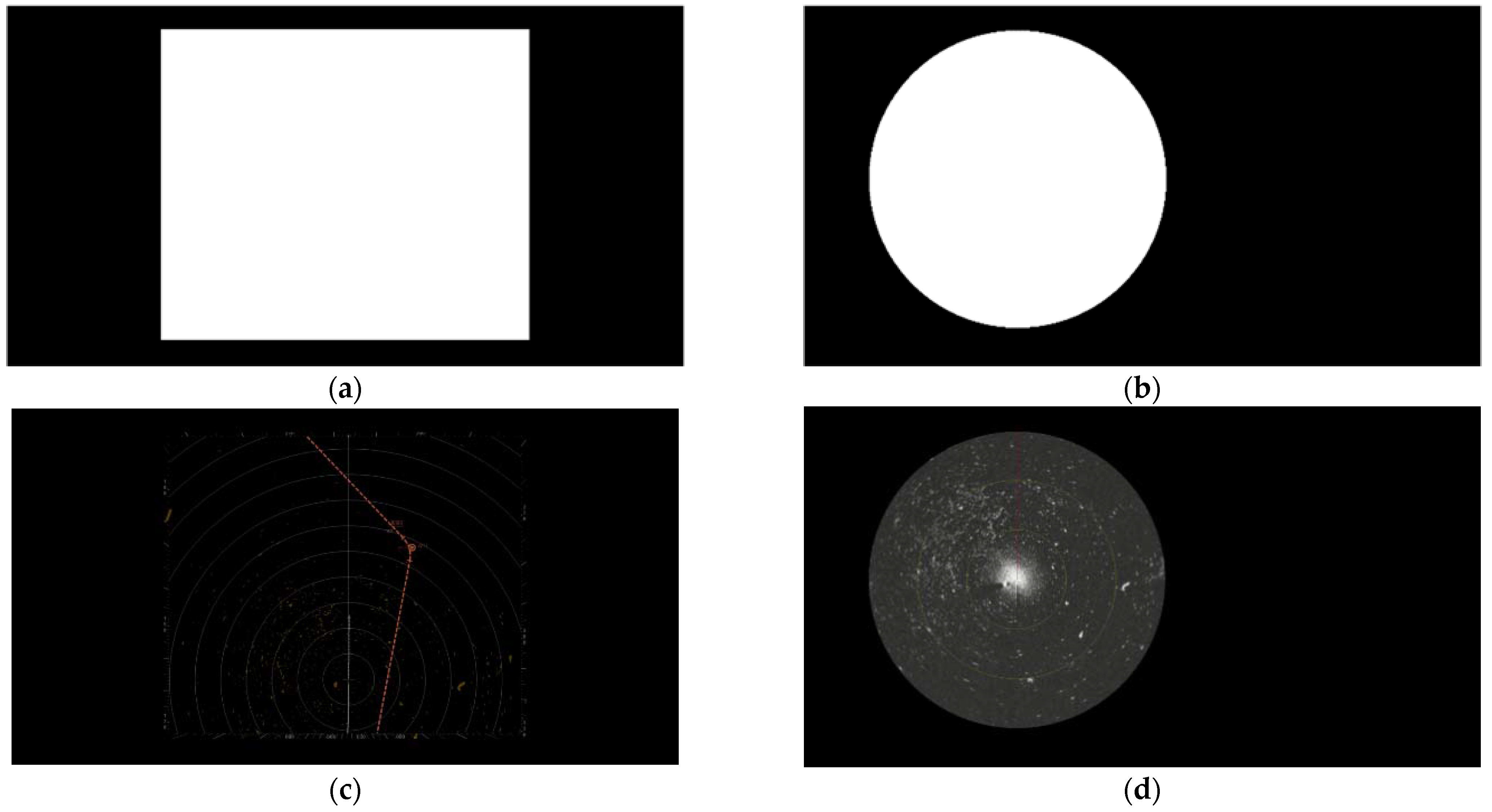
2.2.1. ROI Image Acquisition

According to the basic information such as image size and the range of the ROI obtained from the two original radar images, a mask matrix is created for each of them to display the inside of the ROI in white (with the value set to 1) and the outside of the ROI in black (with the value set to 0), as shown in Figure 4a,b. Then, the image of the ROI can be obtained through Equation (1), as shown in Figure 4c,d.
d s t ( I ) = s r c 1 ( I ) s r c 2 ( I )       i f   m a s k ( I ) 0
where d s t represents the output image matrix;   I represents the multi-dimensional index of elements in the image matrix; s r c 1 and s r c 2 represent two image matrices with the same size; m a s k represents the mask matrix.

2.2.2. Marking Lines and Frames Elimination

In addition to radar echo, there may also be occlusion and the interference of various marking lines and frames in the obtained image of the ROI. For example, in the image of the ROI of the ice radar, there are red heading lines and yellow distance scale rings, as shown in Figure 5a. After creating the mask matrix to mark the areas to be eliminated, as shown in Figure 5b, the result of elimination can indeed improve the influence of the marking lines on radar echo, as shown in Figure 5c.

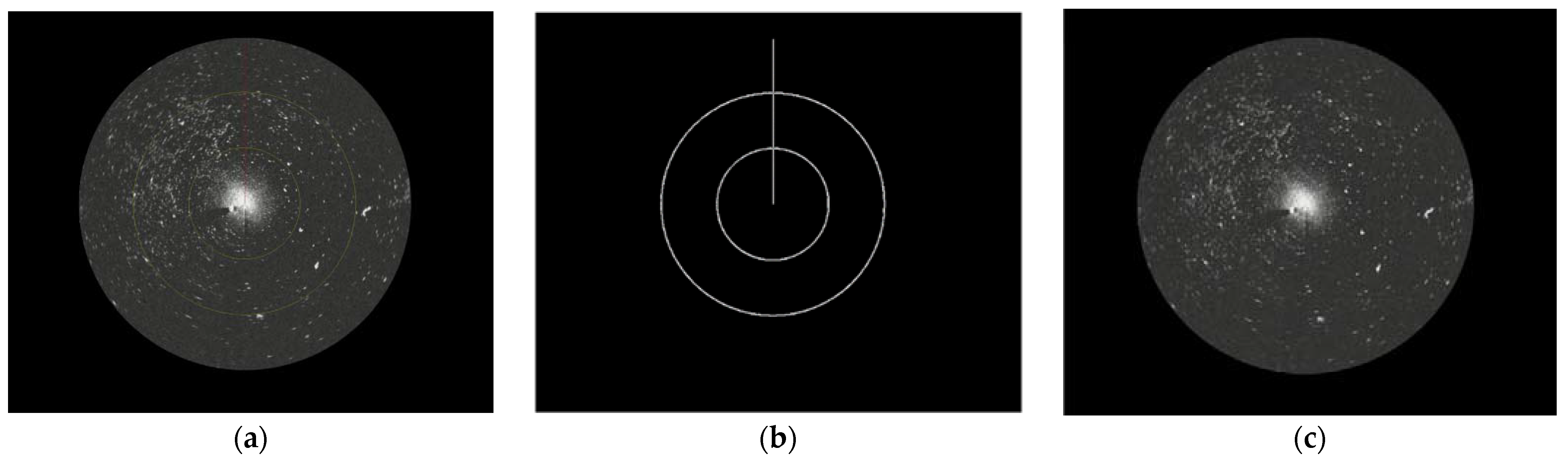
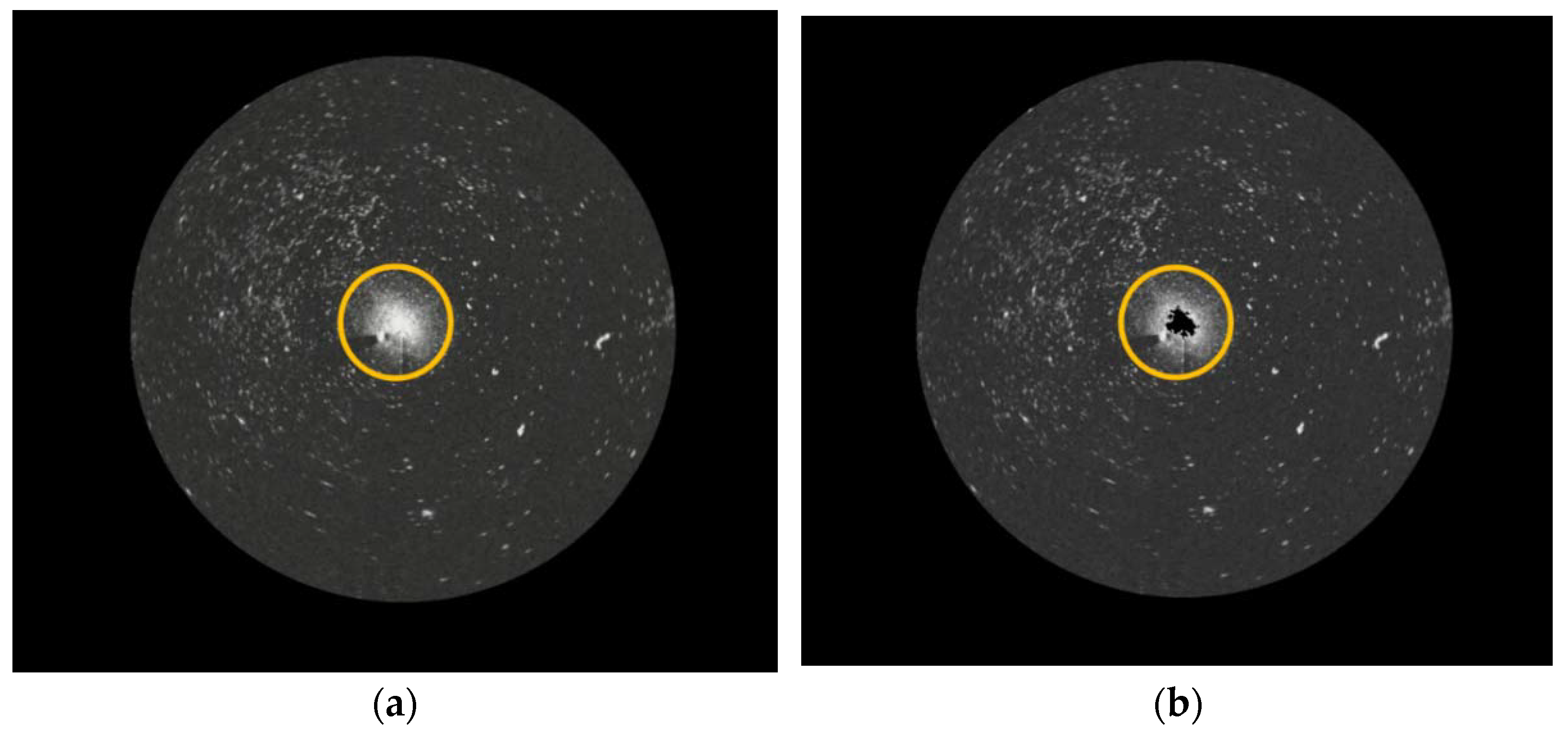
2.2.3. Own-Ship Echo Elimination

When a small and independent echo is displayed at the center of the radar distance scale ring, the echo may be the clutter generated by the steel hull of the own-ship rather than sea ice or other objects. The contour range information of all echoes in the image of the ROI are detected and compared with the position of the own-ship. After confirming the overlapping contour range information, the echo of the own-ship can be eliminated, as shown in Figure 6a,b.

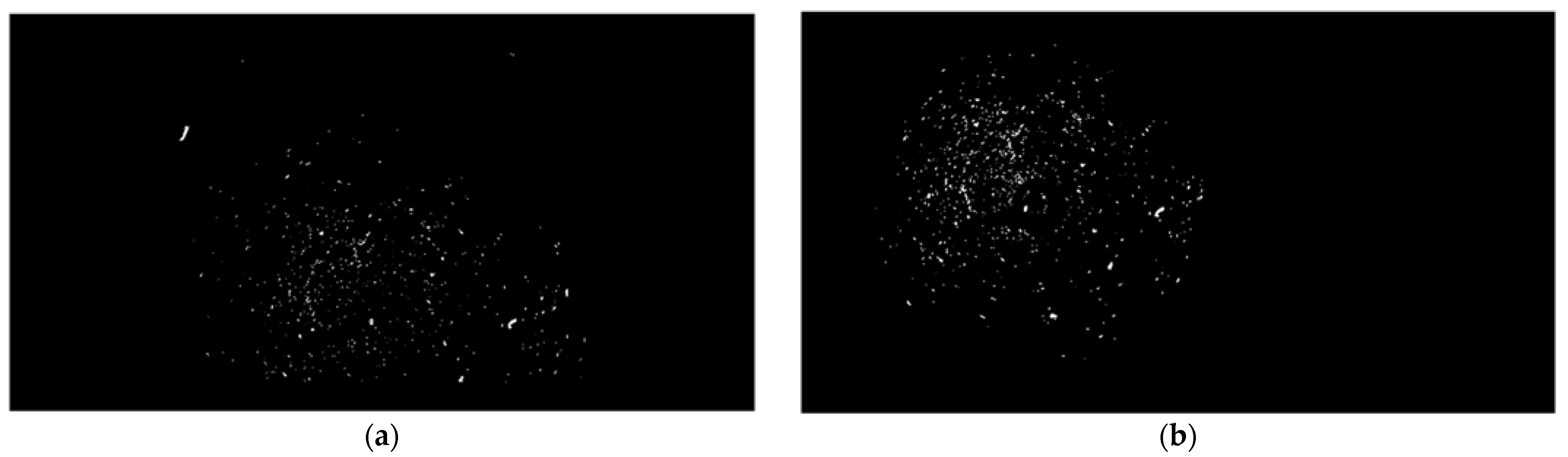
2.2.4. Radar Echo Extraction

The marine radar echo is displayed in orange-yellow and the ice radar echo is displayed in grayish-white. In order to better extract the radar echoes with specific colors, the color space of image of the ROI is converted from RGB to HSV. Then, after setting the corresponding color threshold, the binary radar image can be obtained through Equation (2), as shown in Figure 7a,b.
d s t ( I ) = l o w e r b ( I ) s r c ( I ) u p p e r b ( I )
where d s t represents the output image matrix;   I represents the multi-dimensional index of elements in the image matrix; l o w e r b represents the lower boundary threshold;   s r c represents the input image matrix; u p p e r b represents the upper boundary threshold.

2.3. Spatial Registration Correction

In order to carry out spatial registration correction, this study adopts the method of fixing the marine radar image and adjusting the ice radar image to make a geometric transformation of the ice radar image.

2.3.1. Image Rotation

When the heading angles of the marine radar and ice radar images are inconsistent, after confirming the rotation angle, the image can be rotated through affine transformation of Equation (3) or coordinate transformation of Equations (4) and (5).
For example, if the heading angle of the marine radar image is 0° and the heading angle of the ice radar image is 60°, after rotating the ice radar image counterclockwise by 60°, the same heading angle as the marine radar image can be obtained.
[ u v 1 ] = A [ u v 1 ] = [ cos θ sin θ 0 sin θ cos θ 0 0 0 1 ] [ u v 1 ]
u = u cos θ v sin θ
v = u sin θ + v cos θ
where ( u , v ) represent the pixel coordinates in the transformed image; A represents the affine matrix; ( u , v ) represent the pixel coordinates in the original image; θ represents the rotation angle.

2.3.2. Image Zooming

When the pixel distances corresponding to the same 1 nm of the marine radar and ice radar images are inconsistent, after confirming the zooming ratio, the image can be zoomed through affine transformation of Equation (6) or coordinate transformation of Equations (7) and (8). For example, if 2 nm in the distance scale ring of the marine radar corresponds to 105 px, and 2 nm in the distance scale ring of the ice radar corresponds to 100 px, after magnifying the ice radar image by 1.05 times, the same corresponding pixel distance per nm as the marine radar image can be obtained.
[ u v 1 ] = A [ u v 1 ] = [ c u 0 0 0 c v 0 0 0 1 ] [ u v 1 ]
u = c u u
v = c v v
where ( u , v ) represent the pixel coordinates in the transformed image; A represents the affine matrix; ( u , v ) represent the pixel coordinates in the original image; c u and c v   represent the zooming ratio.

2.3.3. Image Translation

When the pixel positions of the own-ship of the marine radar and ice radar images are inconsistent, after confirming the vertical and horizontal movement values, the image can be translated through affine transformation of Equation (9) or coordinate transformation of Equations (10) and (11). For example, if the pixel position of the own-ship of the marine radar is located at (690, 555), the pixel position of the own-ship of the ice radar is located at (430, 350), and the corresponding pixel distance per nm of the two radar images is the same, after translating the ice radar image to the right by 260 px and downward by 205 px, the same pixel position of the own-ship as the marine radar image can be obtained.
[ u v 1 ] = A [ u v 1 ] = [ 1 0 t u 0 1 t v 0 0 1 ] [ u v 1 ]
u = u + t u
v = v + t v
where ( u , v ) represent the pixel coordinates in the transformed image; A represents the affine matrix; ( u , v ) represent the pixel coordinates in the original image; t u represents the vertical movement value; t v represents the horizontal movement value.

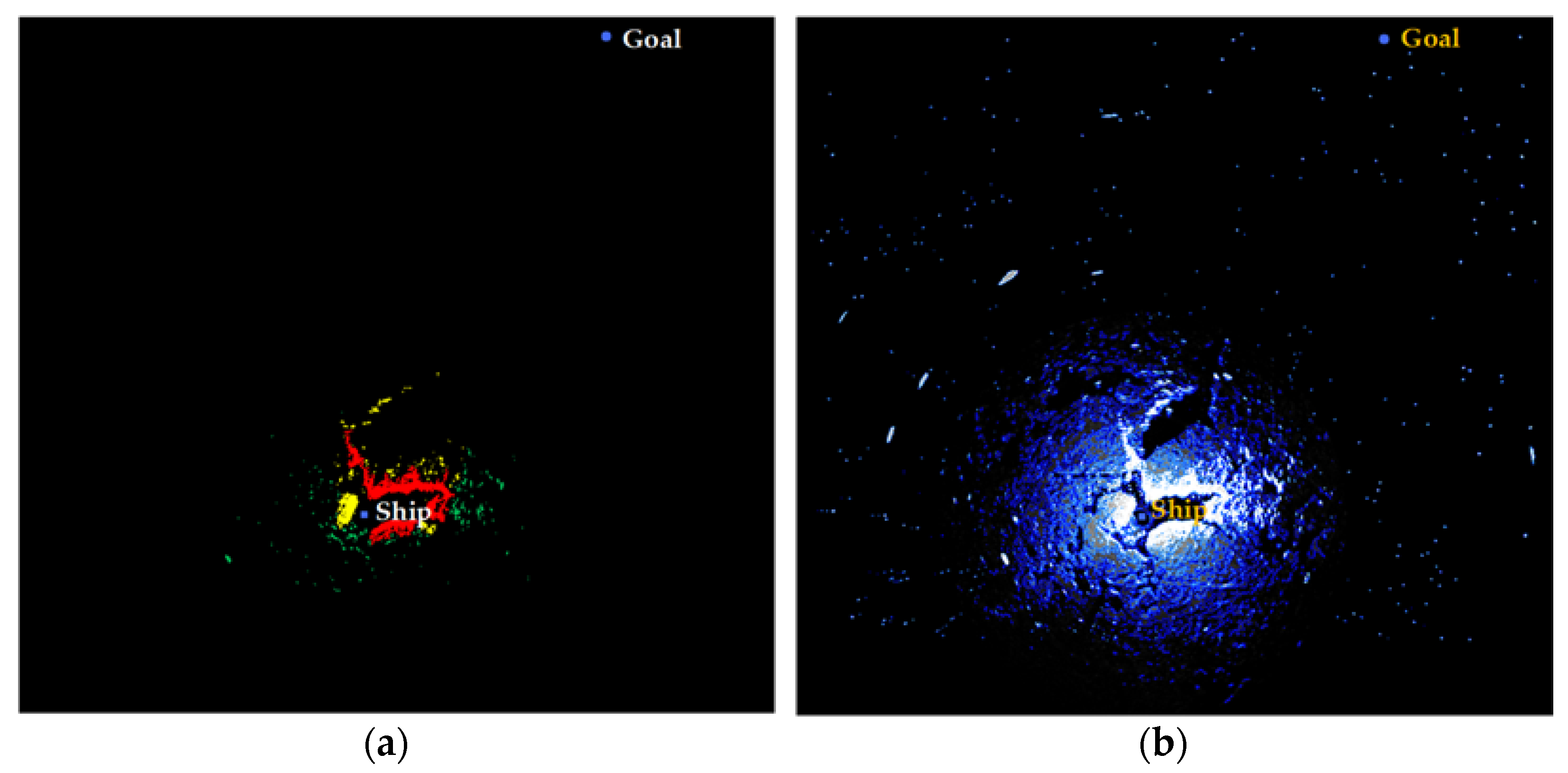
2.4. Radar Image Fusion

After eliminating redundant information and correcting spatial registration, the image fusion can be carried out through Equation (12) after confirming the respective weights of marine radar and ice radar images. The orange-yellow marine radar echo is less sensitive to sea ice perception, but it helps to outline the edge contours of the sea ice, while the grayish-white ice radar echo has a higher sensitivity to sea ice perception. The whiter and brighter the echo color is, the thicker the sea ice thickness is, which helps to master the structure and texture of the sea ice layer. The complementary and combination of the two kinds of radar image information will contribute to the subsequent development of sea ice perception application function.
d s t ( I ) = s r c 1 ( I ) × a l p h a + s r c 2 ( I ) × b e t a + g a m m a
where d s t represents the output image matrix; I represents the multi-dimensional index of elements in image matrix; s r c 1 and s r c 2 represent two image matrices with the same size; a l p h a represents the weight of image 1; b e t a represents the weight of image 2; g a m m a represents the add scalar value.

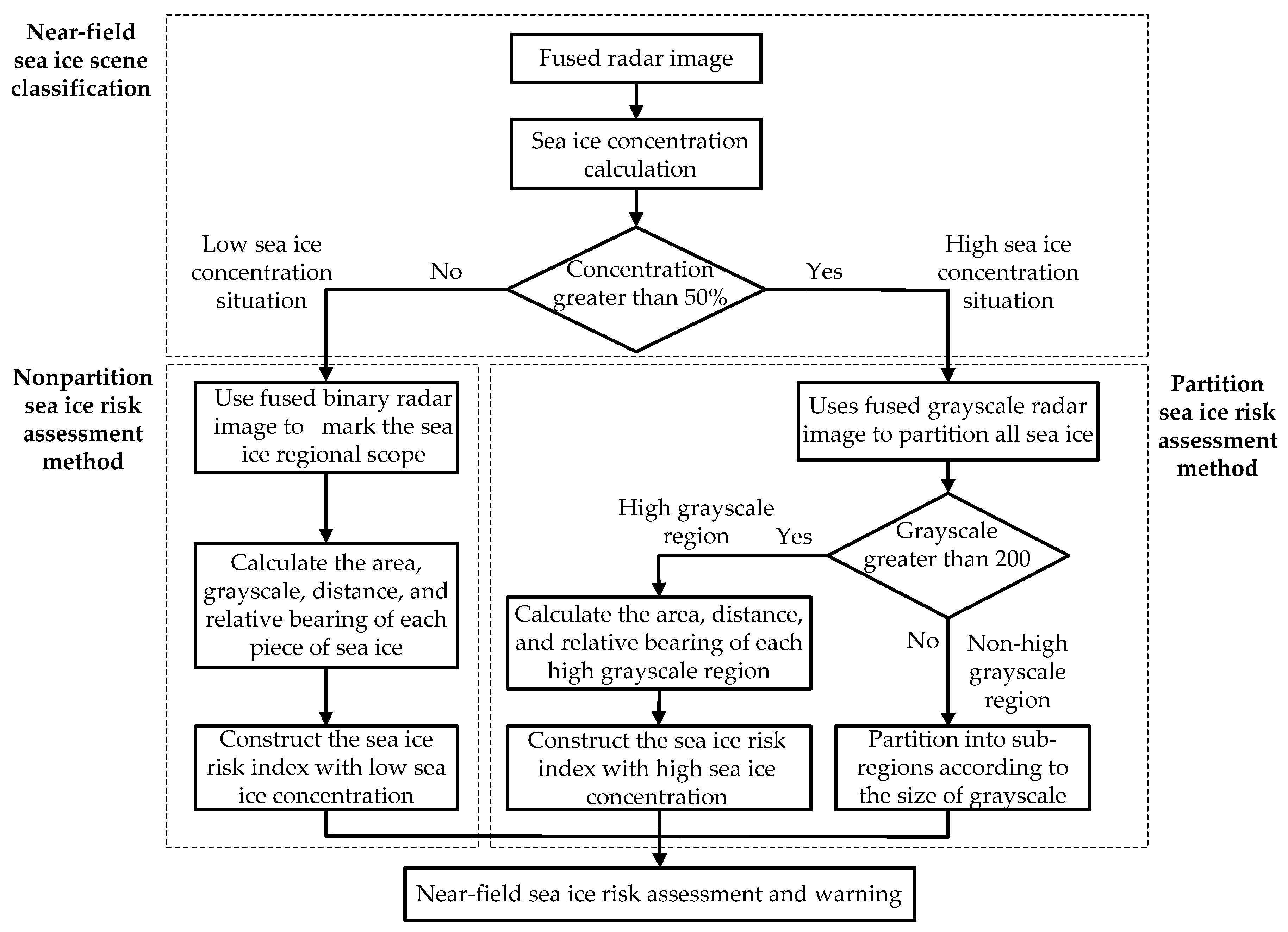
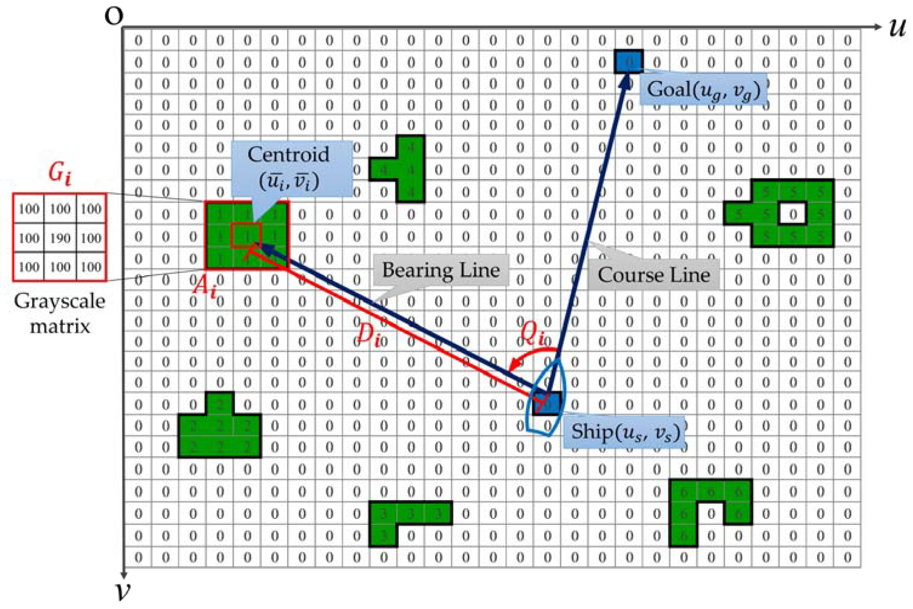
3. Near-Field Sea Ice Risk Assessment and Warning Process

As the ship is sailing, in addition to considering the physical characteristics of near-field sea ice (such as concentration, area, and grayscale), it is more important to consider the relationship between the own-ship and near-field sea ice (such as distance and relative bearing) from the perspective of the navigator. Therefore, this study proposes a set of near-field sea ice risk assessment and warning processes that meet the needs of autonomous ships in the polar region and are suitable for two situations, as shown in Figure 8. By calculating the sea ice concentration of the fused radar image, the near-field sea ice scene with a sea ice concentration less than or equal to 50% is defined as the low-sea-ice-concentration situation, and the near-field sea ice scene with a sea ice concentration greater than 50% is defined as the high-sea-ice-concentration situation. Then, by using the risk variables such as sea ice area, sea ice grayscale, distance between sea ice and the own-ship, and relative bearing of sea ice and the own-ship, the sea ice risk index with low-sea-ice-concentration and the sea ice risk index with high-sea-ice-concentration are constructed. Finally, visualization processing is carried out according to the size of the risk index values of each piece of sea ice to achieve a better near-field sea ice risk assessment and warning effect.

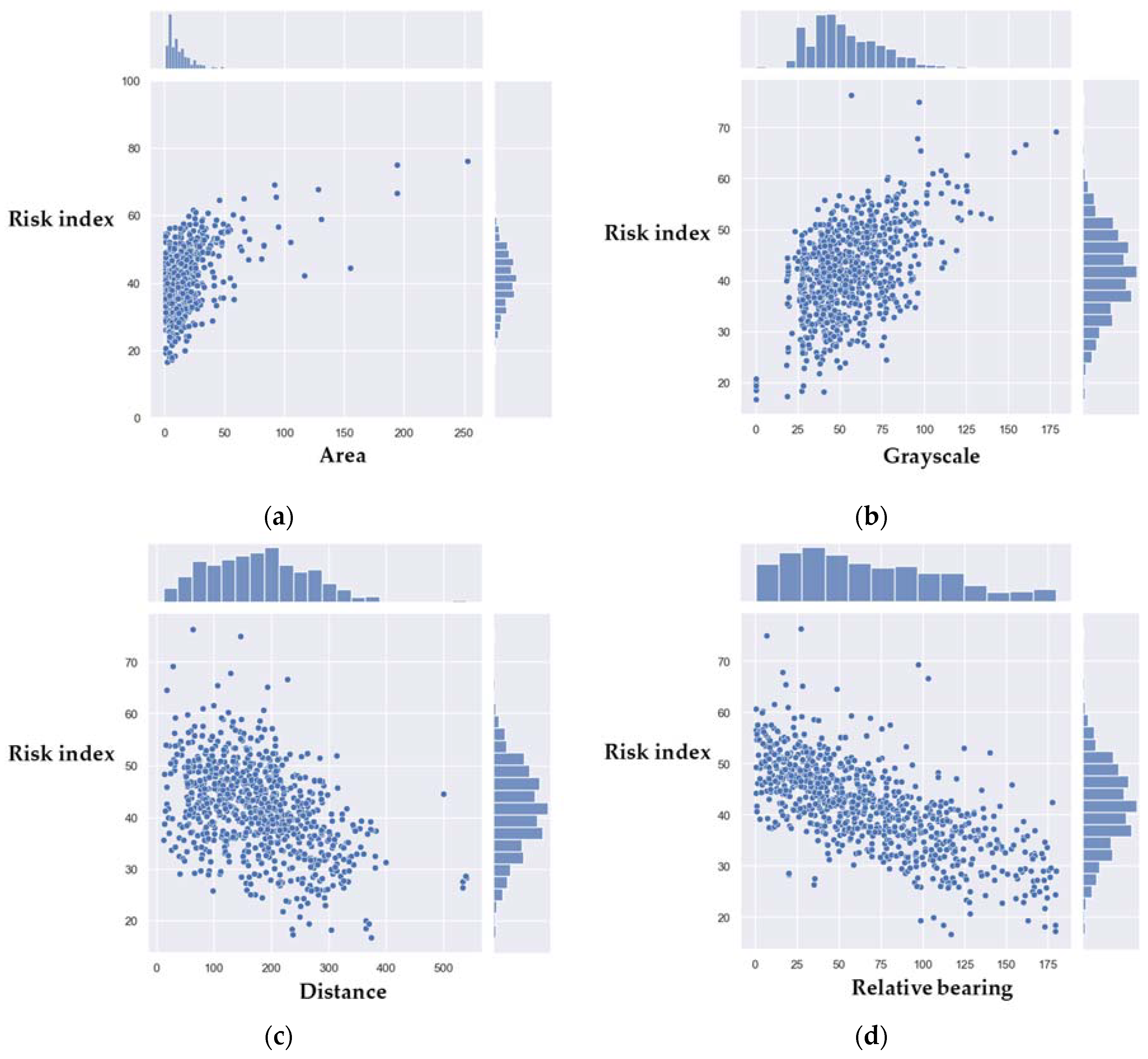
3.1. Near-Field Sea Ice Risk Variables Calculation

3.1.1. Sea Ice Concentration

When calculating the sea ice concentration, the near-field area of the own-ship is defined as a circular area with the position of the own-ship at the center and a radius of 200 px. Then, the sea ice concentration in the near-field area of the own-ship can be obtained through Equations (13) and (14).
c o u n t = I : s r c ( I ) 0 1
S I C = c o u n t π r 2 × 100 %
where c o u n t represents the total number of sea ice pixels (i.e., the elements whose value is not 0 in the image matrix) in the near-field area of the own-ship; I represents the multi-dimensional index of elements in the image matrix; s r c represents the image matrix of the near-field area of the own-ship; S I C represents the value of sea ice concentration in the near-field area of the own-ship.

3.1.2. Sea Ice Area

When calculating the sea ice area, the total number of pixels contained in each piece of sea ice is the area value of the piece of sea ice, which can be obtained through Equation (15). For example, as shown in Figure 9, the sea ice image matrix numbered 1 contains 9 px in total, so the area value of this piece of sea ice is 9.
A i = I : s r c ( I ) = i 1
where A i represents the area value of the i -th piece of sea ice; I represents the multi-dimensional index of elements in the image matrix; s r c represents the sea ice image marker matrix.

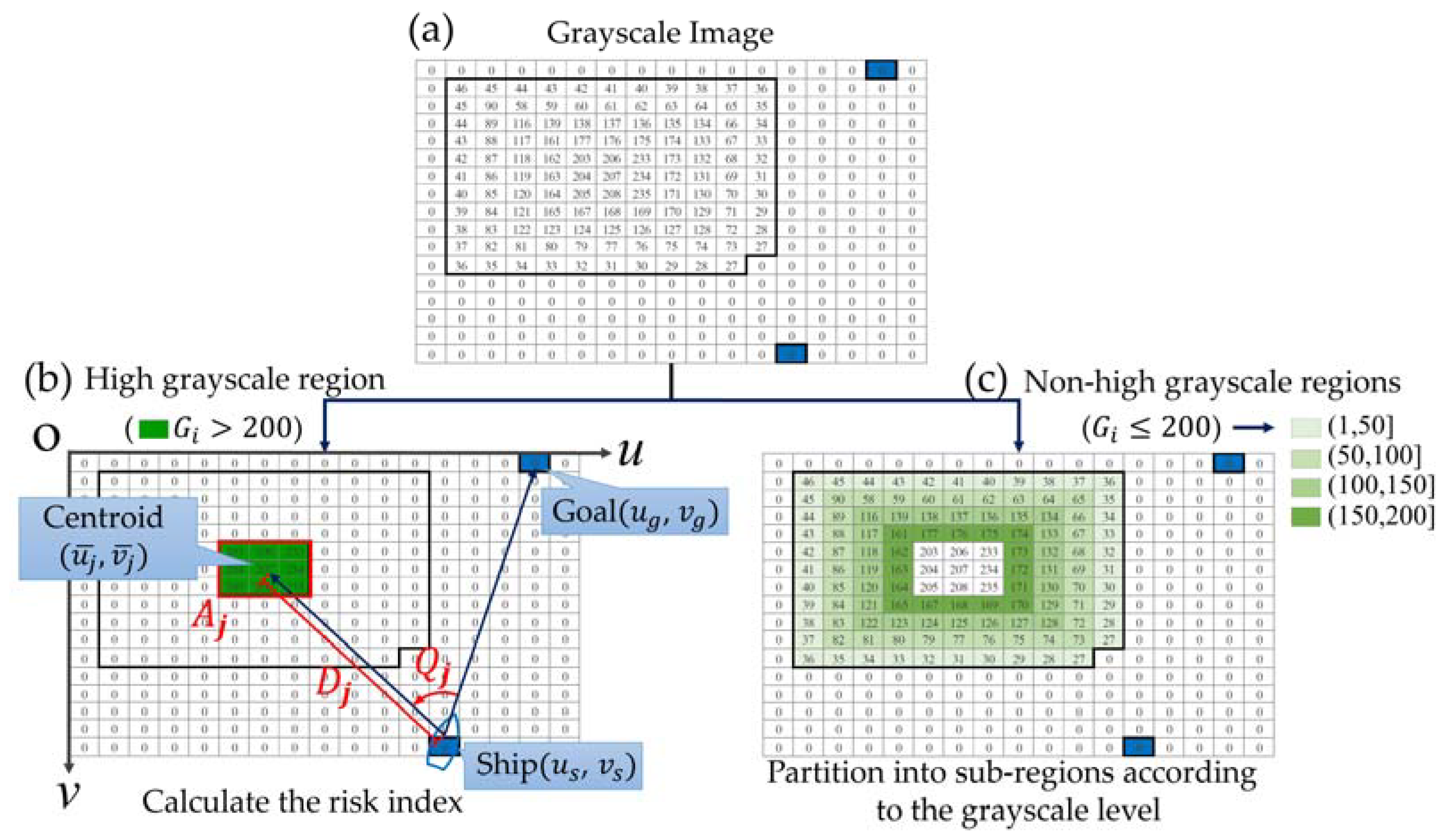
3.1.3. Sea Ice Grayscale

When calculating the sea ice grayscale, the average grayscale value of each piece of sea ice is the grayscale value of the piece of sea ice, which can be obtained through Equations (16) and (17). For example, as shown in Figure 9, the sum of the grayscale values of all pixels in the sea ice image matrix numbered 1 is 990, and the area value is 9, so the average grayscale value of this piece of sea ice is 110. Related studies have shown that there is an exponential relationship between sea ice albedo and sea ice thickness, and some scholars have proposed a retrieval model based on the exponential relationship between sea ice albedo and sea ice thickness [28,29]. Therefore, the higher the grayscale value of sea ice measured from the radar image, the thicker the sea ice may be.
G i _ s u m = I : s r c ( I ) = i G _ b l e n d ( I )
G i = G i _ s u m A i
where G i _ s u m represents the sum of grayscale values of the i -th piece of sea ice; I represents the multi-dimensional index of elements in the image matrix; s r c represents the sea ice image marker matrix; G _ b l e n d represents the grayscale image fused according to a certain weight; G i represents the average grayscale value of the i -th piece of sea ice; A i represents the area value of the i -th piece of sea ice.

3.1.4. Distance between Sea Ice and the Own-Ship

When calculating the distance between sea ice and the own-ship, the distance refers to the Euclidean metric from the centroid of the sea ice to the position of the own-ship. Each piece of sea ice is regarded as an area with uniform mass distribution. The centroid of each piece of sea ice can be obtained through Equations (18) and (19), and then the distance between each piece of sea ice and the own-ship can be obtained through Equation (20). For example, as shown in Figure 9, the distance value between sea ice numbered 1 and the own-ship is 15 px.
u i ¯ =   u i d θ   1 d θ
v i ¯ =   v i d θ   1 d θ
D i = ( u s u i ¯ ) 2 + ( v s v i ¯ ) 2
where ( u i ¯ , v i ¯ ) represents the centroid coordinates of the i -th piece of sea ice; ( u , v ) represents the pixel coordinates of the i -th piece of sea ice; θ A i ; D i represents the distance value between the i -th piece of sea ice and the own-ship; ( u s , v s ) represents the position coordinates of the own-ship.

3.1.5. Relative Bearing of Sea Ice and the Own-Ship

When calculating the relative bearing of sea ice and the own-ship, the relative bearing refers to the included angle between the course line and the bearing line (i.e., the included angle between the line from the position of the own-ship to the short-term target position and the line from the position of the own-ship to the centroid of the sea ice, which is measured to the right or left based on the course line, and the range is 0°~180°), which can be obtained through Equations (21)–(24). For example, as shown in Figure 9, the relative bearing value of sea ice numbered 1 and the own-ship is 64.4°.
a i = ( u s u i ¯ ) 2 + ( v s v i ¯ ) 2
b i = ( u g u i ¯ ) 2 + ( v g v i ¯ ) 2
c i = ( u s u g ) 2 + ( v s v g ) 2
Q i = cos 1 ( a i 2 + c i 2 b i 2 2 a i c i )
where a i represents the distance between the centroid of the i -th piece of sea ice and the position of the own-ship; b i represents the distance between the short-term target position and the centroid of the i -th piece of sea ice; c i represents the distance between the position of the own-ship and the short-term target position; Q i represents the relative bearing value of the i -th piece of sea ice and the own-ship; ( u s , v s ) represents the position coordinates of the own-ship; ( u i ¯ , v i ¯ ) represents the centroid coordinates of the i -th piece of sea ice; ( u g , v g ) represents the coordinates of the short-term target position.

3.2. Nonpartition Sea Ice Risk Assessment Method for Low-Sea-Ice-Concentration Situation

In the low-sea-ice-concentration situation, as shown in the bottom left corner of Figure 8, this study uses the fused binary radar image to mark the regional scope of each piece of sea ice, and calculates its area value, grayscale value, distance value from the own-ship, and the relative bearing value to the own-ship throughs Equations (15)–(24), to construct the near-field sea ice risk index with low-sea-ice-concentration.
The marking of the regional scope of each piece of sea ice is shown in Figure 9. The connected regions of each piece of sea ice are marked with positive integers starting from “1” in sequence, and the other background regions are marked with “0”. The regions marked with the same positive integer belong to the same sea ice region. Then, considering variables such as the area value, grayscale value, distance value from the own-ship, and the relative bearing value to the own-ship of each piece of sea ice, this study constructs the near-field sea ice risk index with low-sea-ice-concentration, as shown in Equation (25). Accordingly, the sea ice risk assessment and warning can be carried out based on the obtained risk index values of each piece of sea ice. The assessment method is to treat each piece of sea ice itself as a whole, without any further partition treatment.
L C R I i = [ A i A m a x + G i G m a x + ( D m a x D i ) D m a x + ( Q m a x Q i ) Q m a x ] 4 × 100 %
where A i represents the area value of the i -th piece of sea ice; A m a x represents the maximum area value in all sea ice regions; G i represents the average grayscale value of the i -th piece of sea ice; G m a x represents the maximum average grayscale value in all sea ice regions; D i represents the distance value between the i -th piece of sea ice and the own-ship; D m a x represents the maximum distance value from the own-ship in all sea ice regions; Q i represents the relative bearing value of the i -th piece of sea ice and the own-ship; Q m a x represents the maximum relative bearing value to the own-ship in all sea ice regions; L C R I i represents the risk index value of the i -th piece of sea ice.

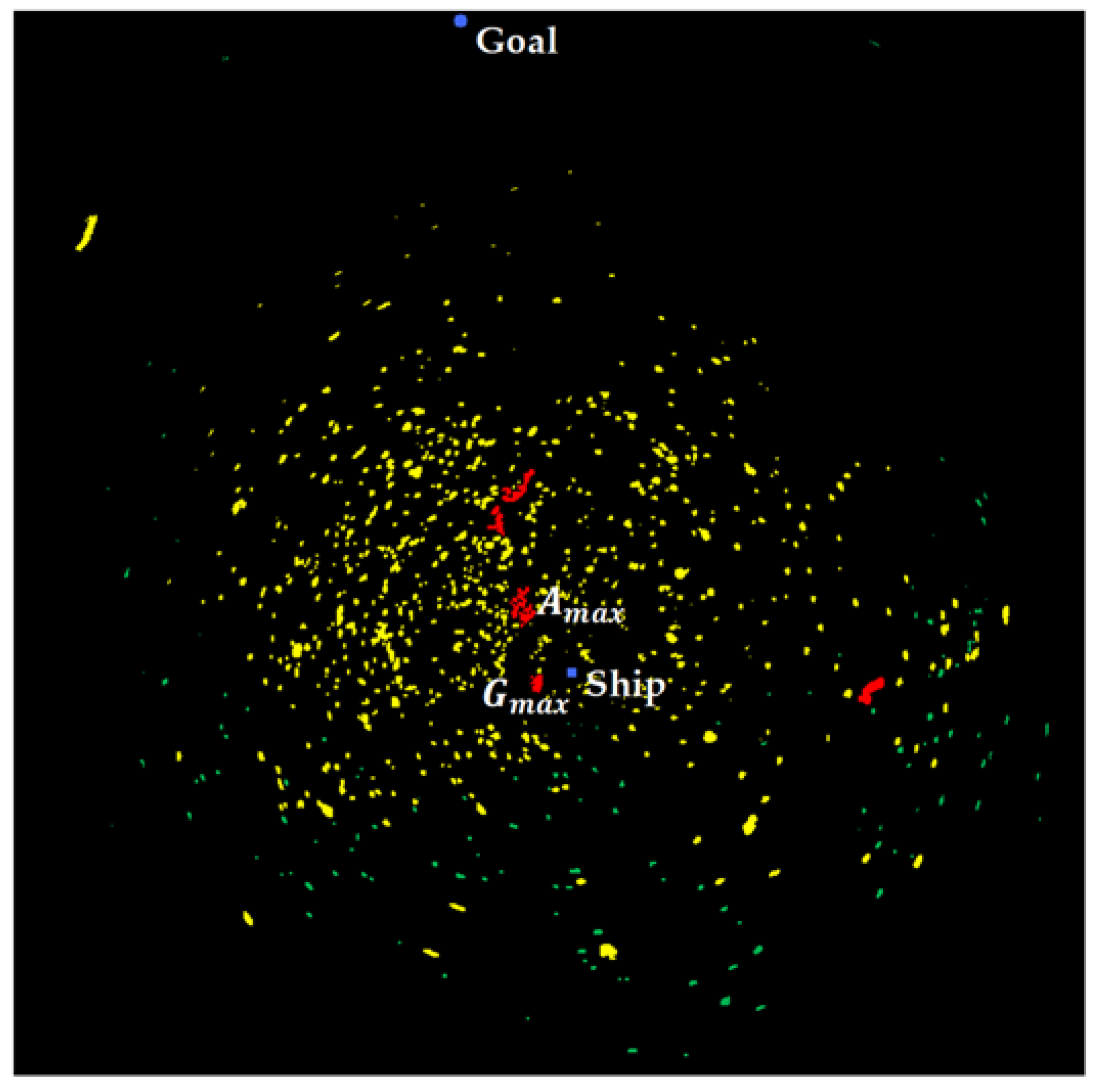
3.3. Partition Sea Ice Risk Assessment Method for High-Sea-Ice-Concentration Situation

In the high-sea-ice-concentration situation, as shown in the bottom right corner of Figure 8, if the risk index is still constructed for the whole sea ice, it is easy to cause the near-field area of the own-ship to be full of high-risk sea ices, and the effect of sea ice risk assessment and warning is poor. Thus, this study uses the fused grayscale radar image to partition all sea ice. The regions with a sea ice grayscale greater than 200 are defined as high grayscale regions, and the other regions with a sea ice grayscale less than or equal to 200 are defined as non-high grayscale regions. Then, for the high grayscale regions in each piece of sea ice, their area value, distance value from the own-ship, and the relative bearing value to the own-ship are calculated through Equations (15) and (18)–(24), to construct the near-field sea ice risk index with high-sea-ice-concentration.
The partition of each piece of sea ice is shown in Figure 10a. For example, there is a large intact sea ice in the front left of the own-ship. According to the size of the grayscale values, it can be partitioned into the high grayscale regions and the non-high grayscale regions. For the high grayscale regions, as shown in Figure 10b, considering variables such as the area value, distance value from the own-ship, and the relative bearing value to the own-ship, this study constructs the near-field sea ice risk index with high-sea-ice-concentration, as shown in Equation (26); although the other non-high grayscale regions do not involve the construction of the near-field sea ice risk index, they can still be partitioned into four sub-regions (e.g., (1,50], (50,100], (100,150], (150,200]) according to the size of the grayscale values, which is helpful for the visualization of subsequent risk warning, as shown in Figure 10c. Accordingly, the sea ice risk assessment and warning can be carried out based on the obtained risk index values of the high grayscale regions in each piece of sea ice. The assessment method is to partition each piece of sea ice to find out the priority regions that have the greatest impact on navigation safety in the whole sea ice.
H C R I j = [ A j 3 A σ + ( D m a x D j ) D m a x + ( 90 Q j ) 90 ] 3 × 100 %
where A j represents the area value of the j -th high grayscale region; A σ represents the standard deviation of the area values of all high grayscale regions; D j represents the distance value between the j -th high grayscale region and the own-ship; D m a x represents the maximum distance value from the own-ship in all high grayscale regions; Q j represents the relative bearing value of the j -th high grayscale region and the own-ship; H C R I j represents the risk index value of the j -th high grayscale region.

4. Example Demonstration for Near-Field Sea Ice Perception and Warning

This study collected the replay videos of marine radar and ice radar of the polar research icebreaker Xuelong 2 from Shenzhen to Zhongshan Station for China’s 36th Antarctic expedition in 2019. The radar images used in subsequent examples of low-sea-ice-concentration and high-sea-ice-concentration were all captured from these radar replay videos of this voyage.

4.1. Example 1

Example 1 used image software to capture the marine radar and ice radar images at 20:39:26 on 18 November 2019, as shown in Figure 11a,b. At this time, Xuelong 2 approached 63° south latitude, and the sea ice distribution was relatively scattered and sparse. Through the radar image fusion process in Section 2, after redundant information elimination, spatial registration correction, and image fusion, the fused radar image obtained is shown in Figure 11c.
In the fused radar image of example 1, through Equations (13) and (14), it can be calculated that the total number of sea ice pixels in the near-field area with the position of the own-ship at the center and a radius of 200 px is 7883, and the obtained sea ice concentration is 6.2% (less than 50%), which belongs to the low-sea-ice-concentration situation. Therefore, by adopting the nonpartition sea ice risk assessment method, the regional scope of each piece of sea ice in the fused binary radar image is marked, and a total of 824 pieces of sea ice can be obtained. The area value, grayscale value, distance value from the own-ship, and the relative bearing value to the own-ship of each piece of sea ice can be calculated through Equations (15)–(24) in Section 3.1. Then, the risk index value of each piece of sea ice can be obtained through Equation (25) in Section 3.2.
By drawing scatter plots, the correlation between the obtained sea ice risk index and each variable is analyzed separately, as shown in Figure 12a,d; the obtained sea ice risk index value ranges from 16.6% to 76.3%. It can be seen from Figure 12a that the minimum value of sea ice area is 1 and the maximum is 253. The larger the sea ice area, the higher the risk, and the two are positively correlated. It can be seen from Figure 12b that the minimum value of sea ice grayscale is 0 and the maximum is 178.3. The greater the sea ice grayscale, the higher the risk, and the two are positively correlated. It can be seen from Figure 12c that the minimum distance value between sea ice and the own-ship is 11.7 and the maximum is 540. The closer the sea ice, the higher the risk, and the two are negatively correlated. It can be seen from Figure 12d that the minimum relative bearing value of sea ice and the own-ship is 0.2°, and the maximum is 179.8°. The smaller the relative bearing (that is, the closer the position is to the front of the own-ship), the higher the risk, and the two are negatively correlated. Based on the above analysis results, the near-field sea ice risk index with low-sea-ice-concentration proposed in this study can indeed reasonably reflect the influence degree of each piece of sea ice on the navigation safety of the own-ship.
According to the size of the obtained risk index values, the regions of each piece of sea ice can be marked with different colors for sea ice risk assessment and visualization warning, as shown in Figure 13. When the sea ice risk index value is greater than 66% ( H C R I j > 66%), the sea ice region is marked in red and belongs to high-risk sea ice that the own-ship should focus on. When the sea ice risk index value is less than or equal to 66% and greater than 33% (33% < H C R I j ≤ 66%), the sea ice region is marked in yellow and belongs to medium-risk sea ice. When the sea ice risk index value is less than or equal to 33% ( H C R I j ≤ 33%), the sea ice region is marked in green and belongs to low-risk sea ice. In addition, the A m a x can be marked next to the sea ice with the largest area and the G m a x can be marked next to the sea ice with the greatest grayscale to more intuitively display the sea ice information that threatens the navigation safety of the own-ship.

4.2. Example 2

Example 2 used image software to capture the marine radar and ice radar images at 13:45:53 on 19 November 2019, as shown in Figure 14a,b. At this time, Xuelong 2 approached 66° south latitude, and the sea ice distribution was relatively concentrated and significant. Through the radar image fusion process in Section 2, after redundant information elimination, spatial registration correction, and image fusion, the fused radar image obtained is shown in Figure 14c.
In the fused radar image of example 2, through Equations (13) and (14), it can be calculated that the total number of sea ice pixels in the near-field area with the position of the own-ship at the center and a radius of 200 px is 96,489, and the obtained sea ice concentration is 76.7% (greater than 50%), which belongs to the high-sea-ice-concentration situation. Therefore, by adopting the partition sea ice risk assessment method, all sea ice regions in the fused grayscale radar image are partitioned into the high grayscale regions with a sea ice grayscale greater than 200 and the non-high grayscale regions with a sea ice grayscale less than or equal to 200. For all high grayscale regions, the area value, distance value from the own-ship, and the relative bearing value to the own-ship can be calculated through Equations (15) and (18)–(24) in Section 3.1. Then, the risk index values of the high grayscale regions in each piece of sea ice can be obtained through Equation (26) in Section 3.2.
According to the size of the obtained risk index values of the high grayscale regions, the same criteria as in Section 4.1 (the risk index value is greater than 66%, less than or equal to 66% and greater than 33%, or less than or equal to 33%) can also be used to mark each high grayscale region in red, yellow, and green, respectively, for sea ice risk assessment and visualization warning, as shown in Figure 15a. Other non-high grayscale regions can also be partitioned into four sub-regions (e.g., (1,50], (50,100], (100,150], (150,200]) according to the size of the grayscale values, and then the high grayscale regions (also regard it as a sub-region) are added to draw the contour map of these five sub-regions and to mark them with gradient colors from blue to white for sea ice risk assessment and visualization warning, as shown in Figure 15b.
Figure 15b shows the overall grayscale distribution of sea ice in the near-field of the own-ship. According to the relevant study results that there is an exponential relationship between sea ice albedo and sea ice thickness [28,29], the higher the grayscale value, the thicker the sea ice may be. Therefore, priority attention should be given to regions marked in white (i.e., the high grayscale regions with a sea ice grayscale greater than 200). Figure 15a shows the risk distribution of these high grayscale regions. These regions are partitioned into three levels according to the size of the risk index values, among which the region marked in red is the region that poses the greatest threat to the navigation safety of the own-ship and should be given more priority attention. It can be seen from the results of visualization warning that in the high-sea-ice-concentration situation, the sea ice situation in the near-field area of the own-ship can be fully mastered from the macro- and micro-perspective through the overall grayscale distribution map of sea ice and the risk distribution map of high grayscale regions.
In this example, if the nonpartition sea ice risk assessment method is still adopted, according to the size of the obtained risk index values, the same criteria as in Section 4.1 can also be used to mark the regions of each piece of sea ice in red, yellow, and green, respectively, for sea ice risk assessment and visualization warning, as shown in Figure 16. However, it can be seen from the results of visualization warning that in the near-field area of the own-ship, the own-ship is surrounded by high-risk sea ice marked in red, and it is impossible to distinguish the priority regions that have the greatest impact on navigation safety and should therefore be given more priority attention. Thus, the nonpartition sea ice risk assessment method adopted in the low-sea-ice-concentration situation is indeed not suitable for the high-sea-ice-concentration situation.

4.3. Results and Discussion

From the above two examples, the radar image fusion process proposed in this study is demonstrated. In example 1, in addition to the occlusion and interference of the marking line and marking frame, the echo noise of the own-ship is particularly significant in the ice radar image. After eliminating redundant information, these problems have been improved. In example 2, the heading angle, the corresponding pixel distance per nautical mile, and the position of the own-ship are inconsistent between the marine radar and the ice radar images. The marine radar display orientation is head-up, the heading angle is 0°, the distance scale ring with a radius of 2 nm corresponds to 53 px, and the position of the own-ship is located at (648, 548); the ice radar display orientation is north-up, the heading angle is 102.4°, the distance scale ring with a radius of 2 nm corresponds to 75 px, and the position of the own-ship is located at (430, 350). After the correction of image rotation, zooming, and translation, these spatial registration problems have been solved obviously. It can be seen from Figure 11c and Figure 14c that the radar image fusion effect in these two examples is good.
In addition, from the above two examples, it also demonstrates a set of near-field sea ice risk assessment and warning processes proposed in this study that meets the needs of autonomous ships in the polar region and is suitable for two situations. In the situation of low-sea-ice-concentration in example 1, because the sea ice distribution is relatively scattered and sparse, each piece of sea ice itself is regarded as a whole without any further partition treatment and the nonpartition sea ice risk assessment method proposed in this study is used to calculate the risk index. In the situation of high-sea-ice-concentration in example 2, because the sea ice distribution is relatively concentrated and significant, the partition sea ice risk assessment method proposed in this study is used to partition each piece of sea ice according to the size of the grayscale values, and then the risk index is calculated for the high grayscale regions (i.e., the priority regions that have the greatest impact on navigation safety). It can be seen from Figure 13 and Figure 15 that the risk assessment and warning effects of near-field sea ice are good in both the low-sea-ice-concentration situation in example 1 and the high-sea-ice-concentration situation in example 2.
In fact, the key to near-field sea ice risk assessment and warning is to identify the “relatively” dangerous sea ice regions around the ship. Unlike obstacles of rigid structures such as islands, reefs, or sunken ships, sea ice belongs to flexible structures that ships can contact or break; and the stronger the icebreaking ability of the ship, the thicker the sea ice that can be contacted. For example, the hull structural strength of the Xuelong 2 meets the PC3 level, and it can continuously break ice at a speed of 2~3 knots under sea conditions of 1.5 m of ice and 0.2 m of snow. Therefore, the ship can set the parameter values in the near-field sea ice risk index calculation formula proposed in this study according to its own conditions. With the support of two kinds of radar image information, the near-field sea ice risk index value obtained in this study is based on variable data such as sea ice concentration, sea ice area, sea ice grayscale, distance between sea ice and the own-ship, and relative bearing of sea ice and the own-ship. Unlike the partial and subjective judgment of the navigator, it can determine the sea ice risk situation in the near-field area of the ship more comprehensively and objectively, providing effective support for the assisted decision-making of autonomous navigation in the polar region.

5. Conclusions

For the navigation safety of autonomous ships in the polar region, this study chooses marine radar and ice radar as the near-field sea ice sensing equipment and proposes the radar image fusion process. The process can integrate the two kinds of radar image information well, solve the problems of redundant information and spatial registration during image fusion effectively, and perceive the sea ice information in the near-field area of the ship more comprehensively than a single sensor can.
Considering the relationship between the own-ship and near-field sea ice from the perspective of the navigator, this study proposes a set of near-field sea ice risk assessment and warning processes that meet the needs of autonomous ships in the polar region and are suitable for two situations. In the low-sea-ice-concentration situation, each piece of sea ice itself is regarded as a whole, and the nonpartition sea ice risk assessment method is adopted to calculate the risk index value of each piece of sea ice. In the high-sea-ice-concentration situation, the partition sea ice risk assessment method is used to find out the high grayscale regions that have the greatest impact on navigation safety in the whole sea ice, and calculate the risk index value of the high grayscale regions in each piece of sea ice.
According to the example demonstration results, through the integrated radar image fusion process and a set of near-field sea ice risk assessment and warning processes proposed in this study, the sea ice risk distribution in the near-field area of the ship can be well obtained in both low- and high-sea-ice-concentration situations. These processes and visualized warning maps can provide effective support for the assisted decision-making of autonomous navigation in the polar region.
On the basis of this study, follow-up research can carry out related work on how to maneuver ships to avoid sea ice at a lower risk. In fact, ship navigation is a dynamic process. The process proposed in this study can be used to master the sea ice risk distribution at each time point in the current navigation environment, and can also be used to evaluate the effect of avoiding sea ice.

Author Contributions

T.-H.H. and S.W. conceived and designed the experiments; B.L. performed the experiments; T.-H.H., B.L. and W.L. analyzed the data; S.W. contributed materials; T.-H.H. and B.L. wrote the paper. All authors have read and agreed to the published version of the manuscript.

Funding

This research was funded by National Key Research and Development Program of China (Grant No. 2021YFC2801003, 2021YFC2801004), National Natural Science Foundation of China (Grant No. 52071199), and Shanghai Science and Technology Innovation Action Plan (Grant No. 21DZ1205803).

Institutional Review Board Statement

Not applicable.

Informed Consent Statement

Not applicable.

Data Availability Statement

Not applicable.

Acknowledgments

The authors would like to express their gratitude to Ning Xu, Yanping Zhao, and Xude Zhang of the China Polar Research Institute for their valuable suggestions on this paper.

Conflicts of Interest

The authors declare no conflict of interest.

References

  1. Stroeve, J.; Notz, D. Changing state of Arctic sea ice across all seasons. Environ. Res. Lett. 2018, 13, 10300110. [Google Scholar] [CrossRef]
  2. England, M.R.; Polvani, L.M.; Sun, L. Robust Arctic warming caused by projected Antarctic sea ice loss. Environ. Res. Lett. 2020, 15, 104005. [Google Scholar] [CrossRef]
  3. Yang, J.; Xiao, C.; Liu, J.; Li, S.; Qin, D. Variability of Antarctic sea ice extent over the past 200 years. Sci. Bull. 2021, 66, 2394–2404. [Google Scholar] [CrossRef]
  4. Guarino, M.V.; Sime, L.C.; Schröeder, D.; Irene, M.V.; Rosenblum, E.; Ringer, M.; Ridley, J.; Feltham, D.; Bitz, C.; Eric, J.S.; et al. Sea-ice-free Arctic during the last interglacial supports fast future loss. Nat Clim Chang. 2020, 10, 928–932. [Google Scholar] [CrossRef]
  5. Wright, R.G. Unmanned and Autonomous Ships—An Overview of Mass, 1st ed.; Routledge Taylor & Francis Group: New York, NY, USA, 2020; pp. 115–144. Available online: https://scholar.google.com/scholar?hl=zh-CN&as_sdt=0%2C5&q=Unmanned+and+autonomous+ships-An+Overview+of+MASS&btnG= (accessed on 9 March 2022).
  6. Tsou, M.C. Multi-target collision avoidance route planning under an ECDIS framework. Ocean Eng. 2016, 121, 268–278. [Google Scholar] [CrossRef]
  7. Skauen, A.N. Quantifying the tracking capability of space-based AIS systems. Adv. Space Res. 2016, 57, 527–542. [Google Scholar] [CrossRef] [Green Version]
  8. Gu, W.; Liu, C.; Yuan, S.; Li, N.; Chao, J.; Li, L.; Xu, Y. Spatial distribution characteristics of sea-ice-hazard risk in Bohai, China. Ann. Glaciol. 2013, 54, 73–79. [Google Scholar] [CrossRef] [Green Version]
  9. Wang, L.; Xu, L.; Clausi, D.A. Sea ice concentration estimation during melt from dual-pol SAR scenes using deep convolutional neural networks: A case study. IEEE Trans. Geosci. Electron. 2016, 54, 4524–4533. [Google Scholar] [CrossRef]
  10. Zeng, T.; Shi, L.; Marko, M.; Cheng, B.; Zou, J.; Zhang, Z. Sea ice thickness analyses for the Bohai Sea using MODIS thermal infrared imagery. Acta Oceanol. Sin. 2016, 35, 96–104. [Google Scholar] [CrossRef]
  11. Spreen, G.; Kaleschke, L.; Heygster, G. Sea ice remote sensing using AMSR-E 89-GHz channels. J. Geophys. Res. 2008, 113, C02S03. [Google Scholar] [CrossRef] [Green Version]
  12. Beitsch, A.; Kaleschke, L.; Kern, S. Investigating high-resolution AMSR2 sea ice concentrations during the february 2013 fracture event in the Beaufort Sea. Remote Sens. 2014, 6, 3841–3856. [Google Scholar] [CrossRef] [Green Version]
  13. Posey, P.G.; Metzger, E.J.; Wallcraft, A.J.; Hebert, D.A.; Allard, R.A.; Smedstad, O.M.; Phelps, M.W.; Fetterer, F.; Stewart, J.S.; Meier, W.N.; et al. Improving Arctic sea ice edge forecasts by assimilating high horizontal resolution sea ice concentration data into the US Navy’s ice forecast systems. Cryosphere 2015, 9, 1735–1745. [Google Scholar] [CrossRef] [Green Version]
  14. Hebert, D.A.; Allard, R.A.; Metzger, E.J.; Posey, P.G.; Preller, R.H.; Wallcraft, A.J.; Phelps, M.W.; Smedstad, O.M. Short-term sea ice forecasting: An assessment of ice concentration and ice drift forecasts using the U.S. Navy’s Arctic Cap Nowcast/Forecast System. J. Geophys. Res. 2015, 120, 8327–8345. [Google Scholar] [CrossRef] [Green Version]
  15. Chi, J.; Kim, H. Prediction of Arctic sea ice concentration using a fully data driven deep neural network. Remote Sens. 2017, 9, 1305. [Google Scholar] [CrossRef] [Green Version]
  16. Xiao, F.; Zhang, S.; Li, J.; Geng, T.; Xuan, Y.; Li, F. Arctic sea ice thickness variations from CryoSat-2 satellite altimetry data. Sci. China Earth Sci. 2021, 64, 1080–1089. [Google Scholar] [CrossRef]
  17. Xu, Y.; Li, H.; Liu, B.; Xie, H.; Burcu, O.C. Deriving Antarctic sea-ice thickness from satellite altimetry and estimating consistency for NASA’s ICESat/ICESat-2 missions. Geophys. Res. Lett. 2021, 48, e2021GL093425. [Google Scholar] [CrossRef]
  18. Yan, Y.; Huang, K.; Shao, D.; Xu, Y.; Gu, W. Monitoring the characteristics of the Bohai sea ice using high-resolution geostationary ocean color imager (GOCI) data. Sustainability 2019, 11, 777. [Google Scholar] [CrossRef] [Green Version]
  19. Haverkamp, D.; Soh, L.K.; Tsatsoulis, C. A comprehensive, automated approach to determining sea ice thickness from SAR data. IEEE Trans. Geosci. Remote. Sens. 1995, 33, 46–57. [Google Scholar] [CrossRef] [Green Version]
  20. Weissling, B.; Ackley, S.; Wagner, P.; Xie, H. EISCAM—Digital image acquisition and processing for sea ice parameters from ships. Cold Reg. Sci. Technol. 2009, 57, 49–60. [Google Scholar] [CrossRef]
  21. Zhang, Q.; Skjetne, R. Image processing for identification of sea-ice floes and the floe size distributions. IEEE Trans. Geosci. Remote. Sens. 2015, 53, 2913–2924. [Google Scholar] [CrossRef]
  22. Parmiggiani, F.; Flores, M.M.; Wadhams, P.; Aulicino, G. Image processing for pancake ice detection and size distribution computation. Int. J. Remote Sens. 2019, 40, 3368–3383. [Google Scholar] [CrossRef]
  23. Renner, A.H.H.; Dumont, M.; Beckers, J.; Gerland, S.; Haas, H. Improved characterisation of sea ice using simultaneous aerial photography and sea ice thickness measurements. Cold Reg. Sci. Technol. 2013, 92, 37–47. [Google Scholar] [CrossRef]
  24. Xu, J.; Wang, H.; Cui, C.; Liu, P.; Zhao, Y.; Li, B. Oil spill segmentation in ship-borne radar images with an improved active contour model. Remote Sens. 2019, 11, 1698. [Google Scholar] [CrossRef] [Green Version]
  25. IMO. International Code for Ships Operating in Polar Waters (Polar Code); IMO: London, UK, 2015; Available online: https://wwwcdn.imo.org/localresources/en/MediaCentre/HotTopics/Documents/POLAR%20CODE%20TEXT%20AS%20ADOPTED.pdf (accessed on 9 March 2022).
  26. Hsieh, T.H.; Wang, S.; Gong, H.; Liu, W.; Xu, N. Sea ice warning visualization and path planning for ice navigation based on radar image recognition. J. Mar. Sci. Technol. 2021, 29, 280–290. [Google Scholar] [CrossRef]
  27. Dumitru, C.O.; Andrei, V.; Schwarz, G.; Datcu, M. Machine Learning for Sea Ice Monitoring from Satellites. In Proceedings of the Photogrammetric Image Analysis & Munich Remote Sensing Symposium, Munich, Germany, 18–20 September 2019; pp. 83–89. [Google Scholar] [CrossRef] [Green Version]
  28. Allison, I.; Brandt, R.E.; Warren, S.G. East Antarctic sea ice: Albedo, thickness distribution, and snow cover. J. Geophys. Res. 1993, 98, 12417–12429. [Google Scholar] [CrossRef]
  29. Su, H.; Wang, Y. Using MODIS data to estimate sea ice thickness in the Bohai Sea (China) in the 2009–2010 winter. J. Geophys. Res. 2012, 117, C10018. [Google Scholar] [CrossRef]
Figure 1. Schematic diagram of radar image fusion process.
Jmse 10 00421 g001
Figure 2. The marine radar image: (a) the original radar image; (b) the obtained basic information.
Jmse 10 00421 g002
Figure 3. The ice radar image: (a) the original radar image; (b) the obtained basic information.
Jmse 10 00421 g003
Figure 4. The radar ROI image acquisition: (a) the marine radar mask image; (b) the obtained marine radar ROI image; (c) the marine radar mask image; (d) the obtained ice radar ROI image.
Jmse 10 00421 g004
Figure 5. The radar marking lines and frames elimination: (a) before elimination; (b) the elimination area; (c) after elimination.
Jmse 10 00421 g005
Figure 6. The radar own-ship echo elimination: (a) before elimination; (b) after elimination.
Jmse 10 00421 g006
Figure 7. The radar echo extraction: (a) the obtained binary marine radar image; (b) the obtained binary ice radar image.
Jmse 10 00421 g007
Figure 8. Schematic diagram of near-field sea ice risk assessment and warning process.
Jmse 10 00421 g008
Figure 9. Schematic diagram of sea ice marking in a low-sea-ice-concentration situation.
Jmse 10 00421 g009
Figure 10. Schematic diagram of sea ice partition in a high-sea-ice-concentration situation: (a) grayscale image; (b) high grayscale region; (c) non-high grayscale regions.
Jmse 10 00421 g010
Figure 11. The radar image of example 1: (a) the original marine radar image; (b) the original ice radar image; (c) the fused radar image.
Jmse 10 00421 g011aJmse 10 00421 g011b
Figure 12. The scatter plot of sea ice risk index vs. variables: (a) the risk index vs. sea ice area; (b) the risk index vs. sea ice grayscale; (c) the risk index vs. sea ice distance; (d) the risk index vs. sea ice relative bearing.
Jmse 10 00421 g012
Figure 13. Schematic diagram of sea ice risk assessment and visualization warning of example 1.
Jmse 10 00421 g013
Figure 14. The radar image of example 2: (a) the original marine radar image; (b) the original ice radar image; (c) the fused radar image.
Jmse 10 00421 g014
Figure 15. Schematic diagram of sea ice risk assessment and visualization warning of example 2: (a) the high grayscale region risk distribution; (b) the overall grayscale distribution.
Jmse 10 00421 g015
Figure 16. Schematic diagram of sea ice risk assessment and visualization warning of example 2 using the nonpartition sea ice risk assessment method.
Jmse 10 00421 g016
Publisher’s Note: MDPI stays neutral with regard to jurisdictional claims in published maps and institutional affiliations.

